
1. Introduction
Butterflies are known for their high aerodynamic performance as they are the only insects that regularly use flapping–gliding flight. They can intersperse gliding flight within their periodic wingbeat, in a similar manner to birds, in order to reduce energy consumption (Muijres et al. Reference Muijres, Henningsson, Stuiver and Hedenström2012). Butterflies hold the record for the longest migratory distance among flying insects. Monarch butterflies, with a wingspan length of approximately 4 cm, migrate from eastern North America to central Mexico in the fall at a speed of approximately 50 km per day over a duration of approximately 75 days, flying more than 3600 km (Brower Reference Brower1996; Reppert & de Roode Reference Reppert and de Roode2018; Tejaswi et al. Reference Tejaswi, Sridhar, Kang and Lee2021). Because of the outstanding aerodynamic performance of butterflies, research on the aerodynamic mechanism of butterfly flight is of great importance for the development of micro unmanned aerial vehicles (Kang et al. Reference Kang, Cranford, Sridhar, Kodali, Landrum and Slegers2018).
Butterflies utilize a wide variety of aerodynamic mechanisms to generate lift and achieve efficient flight. By analysing the flow around free-flying butterflies, Srygley & Thomas (Reference Srygley and Thomas2002) identified that they use a leading-edge vortex, wing rotation and wake capture to achieve lift enhancement. During flapping motion, the wing twisting of a butterfly plays a significant role in enhancing lift, while the camber of the wing has been shown to have little effect on lift (Zheng, Hedrick & Mittal Reference Zheng, Hedrick and Mittal2013). The spanwise twist is capable of preventing the generation of a leading-edge vortex beneath the wing during the upstroke and rapid wing rotation at the end stage of upstroke. Yokoyama et al. (Reference Yokoyama, Senda, Iima and Hirai2013) noticed that both the tip vortex formed during the downstroke and the trailing-edge vortex shed at the end of the downstroke could provide lift for a flapping butterfly model during forward flight. Suzuki, Minami & Inamuro (Reference Suzuki, Minami and Inamuro2015) and Tejaswi et al. (Reference Tejaswi, Sridhar, Kang and Lee2021) constructed flapping wing models including a body and investigated the effect of abdominal undulation on lift generation and energy consumption. They found that the abdominal undulation could reduce energy consumption during hovering flight and forward-climbing flight. Fei & Yang (Reference Fei and Yang2015) observed in a self-propulsion butterfly model that, at low flight speed, the wings could utilize the wake of the downstroke to generate extra thrust at the beginning of the upstroke. The slender tail of the swallowtail butterfly's hindwing has been identified as playing a crucial role in enhancing lift by changing the wake structure into a V-shaped one (Park et al. Reference Park, Bae, Lee, Jeon and Choi2010; Choi et al. Reference Choi, Park, Sagong and Lee2012). The V-shape wake moved the vortex centre towards the upper wing surface, resulting in lift enhancement by the tail of the hindwing (Park et al. Reference Park, Bae, Lee, Jeon and Choi2010). The hindwing tail can enhance the lift coefficient and lift-to-drag ratio by 10 %–20 % at angle of attack greater than  $15^{\circ }$ (Choi et al. Reference Choi, Park, Sagong and Lee2012).
A few studies that distinguished the hindwings of butterflies from their forewings have shed some light on the respective aerodynamic functions of the forewing and hindwing. Le Roy et al. (Reference Le Roy, Cornette, Llaurens and Debat2019a) studied the effect of damage to different areas of the wings on the flight performance of butterflies. They found that damage to the forewing significantly reduced the flight speed and the proportion of glide mode. Jantzen & Eisner (Reference Jantzen and Eisner2008) observed that, among butterflies with their hindwings cut off, both the straight-line and turning accelerations were reduced. Noda, Nakata & Liu (Reference Noda, Nakata and Liu2023) simulated the flow fields around hawkmoth models with and without hindwings and their results showed that the presence of hindwings can enhance thrust during upstrokes. The results of the above work indicate that the interactions between the forewing and hindwing may play important roles in the flapping flight of butterflies.
Although butterflies and dragonflies are both four-winged insects, the forewing–hindwing interaction in butterflies is significantly different from that in dragonflies. The research on forewing–hindwing interaction has focused on dragonflies (Lian et al. Reference Lian, Broering, Hord and Prater2014). With regard to the wing shape, the slot gap between the forewing and hindwing of a butterfly is much narrower than the interval between the forewing and hindwing of a dragonfly, and the aspect ratio of a butterfly is lower than that of a dragonfly. Moreover, in contrast to dragonfly wings, for which there is an obvious phase difference between the forewing and hindwing, butterfly wings flap in synchrony (Betts & Wootton Reference Betts and Wootton1988; Wang & Russell Reference Wang and Russell2007; Jantzen & Eisner Reference Jantzen and Eisner2008; Le Roy, Debat & Llaurens Reference Le Roy, Debat and Llaurens2019b). In the studies based on dragonfly flight, the forewing and hindwing have their own pitch axes (Broering & Lian Reference Broering and Lian2010; Lian et al. Reference Lian, Broering, Hord and Prater2014). The forewings and hindwings of butterflies share a common pitch axis (Ancel et al. Reference Ancel, Eastwood, Vogt, Ithier, Smith, Wood and Kovač2017). Even if the forewing and hindwing are in phase in the studies based on dragonfly flight, there is still a change in relative position between the trailing edge of the forewing and the leading edge of the hindwing during the wingbeat.
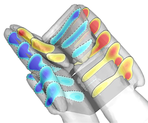
Le Roy et al. (Reference Le Roy, Debat and Llaurens2019b) considered that the slot gap between the butterfly forewing and hindwing may change during a wingbeat owing to the lack of a mechanical connection between the forewing and hindwing. Some analyses of the aerodynamic function of butterfly wings have noted that the forewing and hindwing are on different planes during flight (Le Roy et al. Reference Le Roy, Debat and Llaurens2019b; Johansson & Henningsson Reference Johansson and Henningsson2021). This phenomenon implies the existence of a dihedral angle between the forewing and hindwing planes during flapping flight. This non-zero dihedral angle can be observed in figure 1. A forewing and hindwing with non-zero dihedral angle can be regarded as tandem wings, which can cause forewing–hindwing interaction.
(a) The dihedral angle between the forewing and hindwing during flapping flight of a butterfly. This picture references the movie at the link here. (b) Schematic diagram of the dihedral angle between the forewing and hindwing.

The dihedral angle of the forewing to the hindwing results in a slot near the root of the wing similar to the slotted flap, and a slotted wingtip near the tip of the wing. It is well known that a slotted flap at the trailing edge delays flow separation by transferring high-momentum fluid from the lower surface of the main airfoil to the flap, resulting in a higher lift coefficient on the main airfoil (Petz & Nitsche Reference Petz and Nitsche2007). Slotted wingtips have also been utilized to reduce drag and obtain additional thrust during the gliding process (Withers Reference Withers1981; Tucker Reference Tucker1995; March, Bradley & Garcia Reference March, Bradley and Garcia2005). Slotted wingtips have been shown to improve lift and provide an advantageous lift-to-drag ratio for steady flight in most studies (Tucker Reference Tucker1993; Hossain et al. Reference Hossain, Rahman, Iqbal, Ariffin and Mazian2012; Liu et al. Reference Liu, Song, Yang, Yang, Xue and Lang2021). Liu et al. (Reference Liu, Song, Yang, Xue and Lang2022) pointed out that the slotted wingtip is more favourable in improving lift than an unslotted wing during flapping motion. Especially for low-aspect-ratio wings, it has been found that tip vortices have significant effects on the wake structure and the forces acting on the wings (Taira & Colonius Reference Taira and Colonius2009a,Reference Taira and Coloniusb; Deng & Caulfield Reference Deng and Caulfield2015). However, it has not yet been possible to explain or predict the aerodynamic effects of the slot between the forewing and hindwing during butterfly flight. It is therefore worthwhile exploring whether a wing slot can be utilized to enhance the lift of a low-aspect-ratio flapping wing.
In this paper, we investigate the effect of the slot on lift by using a butterfly-inspired flapping wing model. The flapping wing model consists of a rectangular plate wing with a spanwise slot. The lift coefficients and vortex structures are investigated for cases with different slot parameters by numerical simulations. The slot gap is quantitatively controlled by setting the dihedral angle between the forewing and hindwing. The results show that the dihedral angle between the forewing and hindwing significantly affects aerodynamic performance. A negative dihedral angle (anhedral) significantly enhances lift. The enhanced lift is caused by the streamwise ram effect and tip-vortex capture.
The remainder of the paper is organized as follows. The butterfly-inspired flapping wing model with a spanwise slot and the numerical methods are introduced in § 2. The aerodynamic differences caused by the spanwise slot are discussed in detail and the underlying vortex dynamics is analysed for these differences from the perspective of the vortex lift in § 3. Finally, the conclusions are drawn in § 4.
2. Model and methods
2.1. Butterfly-inspired flapping wing model with a spanwise slot
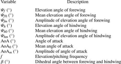
As shown in figure 2, the butterfly-inspired flapping wing model in this paper is constructed based on the rectangular butterfly-like model of Suzuki et al. (Reference Suzuki, Minami and Inamuro2015). The aspect ratio of the model is taken from the relevant butterfly data provided by Le Roy et al. (Reference Le Roy, Amadori, Charberet, Windt, Muijres, Llaurens and Debat2021). The total chord length  $c$ of the model is set to 1, and the wingspan of the forewing is the same as that of the hindwing, namely
 $0.475c$. In figure 2(b), the left and right wings are rotated around the axes
 $F'E'$ and
 $FE$, respectively, to achieve flapping motion. The forewing elevation angle
 $\varPsi _{f}$, the hindwing elevation angle
 $\varPsi _{h}$ and the angle of attack
 $({\rm AoA})$ of the model are given by
 \begin{gather} \varPsi_{f} ={-}\varPsi_{fm}\cos(2{\rm \pi} ft) + \varPsi_{f0}, \end{gather}
 \begin{gather}\varPsi_{h} ={-}\varPsi_{hm}\cos(2{\rm \pi} ft) + \varPsi_{h0}, \end{gather}
 \begin{gather}{\rm AoA} = {\rm AoA}_{m}\sin(2{\rm \pi} ft) + {\rm AoA}_{0}, \end{gather}
where  $f$ is the dimensionless frequency,
 $\varPsi _{fm}$ and
 $\varPsi _{hm}$ are the amplitudes of the elevation angles of the forewing and hindwing,
 $\varPsi _{f0}$ and
 $\varPsi _{h0}$ are the mean values of the elevation angles and
 ${\rm AoA}_m$ and
 ${\rm AoA}_0$ are, respectively, the amplitude and mean value of the angle of attack. These kinematic parameters of the model are summarized in table 1. In this paper, with reference to the parameter settings of elevating and pitching motion given in Suzuki et al. (Reference Suzuki, Minami and Inamuro2015), the elevation amplitudes
 $\varPsi _{fm}=\varPsi _{hm}$ are taken as
 $40^\circ$ and the angles of attack
 ${\rm AoA}_m={\rm AoA}_0$ are taken as
 $15^\circ$. The definition of the dihedral angle on a winglet in Shelton et al. (Reference Shelton, Tomar, Prasad, Smith and Komerath2006) is adopted in this paper to describe the angle between the forewing plane and the hindwing plane. Since the elevation amplitudes of the forewing and hindwing are the same, the dihedral angle
 $\beta$ is given by
 \begin{equation} \beta = \varPsi_{h0} - \varPsi_{f0}. \end{equation}
The dihedral angle  $\beta$ reflects the angle at which the hindwing is upturned relative to the forewing during a wingbeat.
Schematics of the butterfly-inspired flapping wing model. (a) Tiled diagram of the model, consisting of three parts: forewing, hindwing and body. We use a coordinate system  $O$–
 $xyz$ fixed to the body centre to describe the model kinematics. The total chord length of the model is denoted by
 $c$ and the interval from point
 $B$ to point
 $C$ in the
 $x$ direction is
 $0.05c$. The streamwise position
 $x_{s}$ of the slot is equal to 0 for the flapping wing model shown. The slot represents the separation of the forewing and hindwing. The slot position
 $x_{s} = 0$ means that the area of the forewing is equal to that of the hindwing. (b) Front view of the model. Here,
 $\varPsi _{h}$ and
 $\varPsi _{f}$ are the elevation angles of the hindwing and forewing, respectively, and
 $\beta$ denotes the dihedral angle of the hindwing relative to the forewing. When the hindwing is higher than the forewing, the dihedral angle is positive. The figure shows the case of a negative dihedral angle. The body width
 $D_{body}$ is equal to
 $0.05c$. (c) Side view of the model. The angle of attack (
 ${\rm AoA}(t)$) of the body is the angle between the line
 $FE$ and the
 $x$ axis, and the model, which is fixed at point
 $O$, rotates around the
 $y$ axis. The angles of attack of the spanwise slice of the forewing and hindwing are always the same during a wingbeat. (d) Snapshots of the model with dihedral angles
 $\beta =-10^{\circ }$ (left) and
 $\beta =0^{\circ }$ (right). During a wingbeat, the dihedral angle
 $\beta$ remains constant. The wing is coloured by the normalized height
 $z/c$.

Kinematic parameters of butterfly-inspired flapping wing.

2.2. Lift decomposition
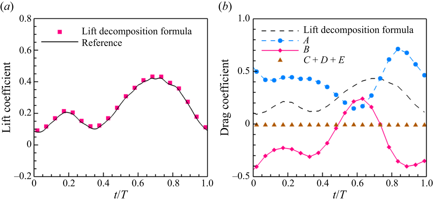
To analyse the aerodynamic forces acting on the wing by the fluid, a force decomposition formula is applied. According to our previous work (Wang et al. Reference Wang, Zhang, He and Liu2013b, Reference Wang, Zhang, He and Liu2015b; Tong, Yang & Wang Reference Tong, Yang and Wang2021), the forces acting on the object can be expressed as follows:
 \begin{align} \boldsymbol{F} &= \rho\int_{V_{f}}\boldsymbol{u}\times\boldsymbol{\omega}\,\mathrm{d}V - \rho\int_{V_{f}}\frac{\partial{\boldsymbol{u}}}{\partial{t}}\,\mathrm{d}V \nonumber\\ &\quad -\oint_{\varSigma}\left(p+\frac{\rho q^2}{2}\right)\boldsymbol{n}\,\mathrm{d}S+\oint_{\varSigma}\boldsymbol{\tau} \,\mathrm{d}S - {\rho} \oint_{\partial{B}}\left(\frac{q^2}{2}\right)\boldsymbol{n}\,\mathrm{d}S, \end{align}
where  $\rho$ is the density,
 $\boldsymbol {u}$ is the velocity,
 $\boldsymbol {\omega }$ is the vorticity,
 $p$ is the pressure,
 $q=|\boldsymbol {u}|$,
 $\boldsymbol {\tau }$ is the viscous shear stress vector on the surface of the control volume,
 $\boldsymbol {\tau }={\mu }\boldsymbol {\omega }\times \boldsymbol {n}$. Also,
 $\mu$ is the fluid dynamic viscosity,
 $\boldsymbol {n}$ is the unit normal vector pointing to the outside of the control surface,
 $V_{f}$ is the control volume,
 $\varSigma$ is its surface and
 $\partial {B}$ is the solid boundary of the object.
When (2.5) is applied in the  $z$ direction to calculate the lift on the object, selecting a suitable control volume can eliminate some of the terms in this equation. When the outer surface of the control volume,
 $\varSigma$, is selected as a rectangle, only the surface integrals over the upper and lower surfaces remain in the third term on the right-hand side of (2.5), because the outer normal vector on the other four surfaces is perpendicular to the
 $z$ axis. If the top and bottom surfaces of the control volume are sufficiently far from the wing, the terms
 $p+{\rho q^2}/{2}$ on the top and bottom surfaces are close enough and can be eliminated according to the Bernoulli equation (
 $P=p+{\rho q^2}/{2}\rightarrow \text {const}$). When the control surface is far enough from the wall, the viscous shear stress term in the
 $z$ direction is nearly zero over most of the control surface in this work, except for the wake region. As shown in figure 18(b) of Appendix A, the fourth term on the right-hand side of (2.5) has been shown to be negligible compared with the first and second terms. The fifth term on the right-hand side is determined by the velocity of motion of the wing. For an infinitely thin airfoil, the fifth term is also negligible compared with the first and second terms. Hence, by selecting a special control volume, the following simplified formula for the lift can be derived:
 \begin{equation} L = \rho\int_{V_{f}} (\boldsymbol{u}\times\boldsymbol{\omega})_z \,\mathrm{d}V - \rho\int_{V_{f}} \left(\frac{\partial \boldsymbol{u}}{\partial t}\right)_z \mathrm{d}V, \end{equation}
where the first term on the right-hand side is the volume integral of the Lamb vector in the vertical direction, representing the vortex lift. The second term on the right-hand side is the volume integral of the local acceleration of the fluid in the vertical direction induced by the motion of the solid wall (Wang et al. Reference Wang, Zhang, He and Liu2013b). The rectangular control volume used in the present work for the lift of the total wing is  $[-4c,(1+\sqrt {3})c/4]\times [-6c,6c]\times [-6c,6c]$ in the streamwise (x), spanwise (y) and vertical (z) directions, respectively. More details of the aerodynamic force decomposition can be found in Appendix A and our previous work (Wang et al. Reference Wang, Zhang, He and Liu2013b, Reference Wang, Zhang, He and Liu2015b; Tong et al. Reference Tong, Yang and Wang2021).
2.3. Numerical method and simulation set-up
The flow around the butterfly-inspired flapping wing is simulated by solving the Navier–Stokes equations on an Eulerian mesh using a semi-implicit immersed boundary method based on the discrete streamfunction formulation (Wang & Zhang Reference Wang and Zhang2011; Wang, He & Zhang Reference Wang, He and Zhang2013a). The continuity equation and the time-dependent three-dimensional incompressible Navier–Stokes equations are taken as the governing equations
 \begin{gather} \boldsymbol{\nabla}\boldsymbol{\cdot}\boldsymbol{u} = 0, \end{gather}
 \begin{gather}\frac{\partial \boldsymbol{u}}{\partial t} + \boldsymbol{u} \boldsymbol{\cdot} \boldsymbol{\nabla} \boldsymbol{u} ={-}\boldsymbol{\nabla} p + \frac{1}{Re} \nabla^2 \boldsymbol{u} + \boldsymbol{f}_{IB}, \end{gather}
where  $\boldsymbol {u}$ is the dimensionless velocity,
 $p$ is the dimensionless pressure,
 $t$ is the dimensionless time,
 $\boldsymbol {\nabla }$ is the gradient operator,
 $\nabla ^2$ is the Laplacian operator,
 $Re$ is the Reynolds number and
 $f_{IB}$ represents the influences of the model on the fluid in the immersed boundary method. The uniform upstream velocity
 $U_\infty$ and the total chord length
 $c$ are taken as the reference velocity and reference length, respectively. The Reynolds number is defined as
 $Re = U_\infty c/\nu$, where
 $\nu$ is the fluid kinematic viscosity.
The spatial discretization is performed using a second-order finite volume method. The time integration adopts a three-step second-order, low-storage Runge–Kutta method. In every substep, the convective term and viscous term in the momentum equation are solved explicitly and implicitly, respectively. The force density  $\boldsymbol {f}_{IB}$ on the Eulerian mesh in (2.8) is calculated using the Lagrangian direct forcing method. The force density
 $\boldsymbol {F}_{IB}$ at the Lagrangian points on the thin-wing model and the force density
 $\boldsymbol {f}_{IB}$ at the Eulerian points are related as follows:
 \begin{equation} \boldsymbol{f}_{IB} = \int_S \boldsymbol{F}_{IB}(\boldsymbol{X},t)\delta(\boldsymbol{x}-\boldsymbol{X})\,\mathrm{d}S, \end{equation}
where  $S$ is the control surface in Lagrangian coordinates,
 $\boldsymbol {X}$ denotes the point position of the Lagrangian mesh and
 $\boldsymbol {x}$ denotes the point position of the Eulerian mesh. Here,
 $\delta (\boldsymbol {x}-\boldsymbol {X})$ is a normalized delta function in three-dimensional space, the expression for which is
 \begin{equation} \delta(\boldsymbol{x}-\boldsymbol{X}) = \frac{1}{h^3} \phi\left(\frac{x-X}{h}\right)\phi\left(\frac{y-Y}{h}\right)\phi\left(\frac{z-Z}{h}\right), \end{equation}
where  $h$ is the minimum size of the Eulerian mesh,
 $(x,y,z)$ and
 $(X,Y,Z)$ are, respectively, the Eulerian and Lagrangian position vectors in the ground coordinate system and the segmentation function
 $\phi$ can be found in our previous work (Wang & Zhang Reference Wang and Zhang2011).
In order to improve the imposition of the no-slip and no-penetration boundary conditions, the forcing term  $\boldsymbol {F}_{IB}(\boldsymbol {X}_j,t)$ at the Lagrangian points is determined implicitly by solving a linear system as follows:
 \begin{equation} \sum_{j=1}^{M} \left(\sum_{\boldsymbol{x}}\delta(\boldsymbol{x}-\boldsymbol{X}_j)\delta(\boldsymbol{x}-\boldsymbol{X}_k) \Delta s h^3\right)\boldsymbol{F}_{IB}(\boldsymbol{X}_j,t) =\frac{\boldsymbol{U}_{b}^{n+1}(\boldsymbol{X}_k)-\boldsymbol{U}_{b}^{*}(\boldsymbol{X}_k)}{\Delta t}, \end{equation}
where  $M$ denotes the number of Lagrangian points and
 $\Delta s$ is the surface area associated with each Lagrangian point. Here,
 $\boldsymbol {X}_k$ and
 $\boldsymbol {X}_j$ are the positions of the Lagrange points
 $k$ and
 $j$, respectively,
 $\boldsymbol {U}_{b}^{n+1}$ is the velocity at the Lagrangian point, obtained from the given motion of the wall and
 $\boldsymbol {U}_{b}^{*}$ is the predicted velocity at the Lagrangian points, the expression for which is
 \begin{equation} \boldsymbol{U}_b^{*}(\boldsymbol{X},t) = \int_V\boldsymbol{u}^{*}(\boldsymbol{x},t)\delta(\boldsymbol{x}-\boldsymbol{X})\,\mathrm{d}V, \end{equation}
where  $\boldsymbol {u}^{*}$ is the velocity at the Eulerian mesh.
More details of the numerical method can be found in our previous papers (Wang & Zhang Reference Wang and Zhang2011; Wang et al. Reference Wang, He and Zhang2013a). The numerical method used in this work has been validated in some similar moving boundary problems in our previous work (Wang et al. Reference Wang, Zhang, He and Liu2013b, Reference Wang, Zhang, He and Liu2014, Reference Wang, Xu, Zhang and Wang2021).
In the present work, the simulations are conducted at a Reynolds number  $Re =300$. The choice of Reynolds number follows that in previous studies (Wang Reference Wang2000; Dong et al. Reference Dong, Mittal, Bozkurttas and Najjar2005; Wang et al. Reference Wang, Xu, Zhang and Wang2021) and is made because the topology of the wake generated by flapping motion for a sharp leading edge is not sensitive to the Reynolds number (Taira & Colonius Reference Taira and Colonius2009b). The increase of the Reynolds number up to
 $O(10^3)$ might affect the evolution of the small-scale vortices, while the large-scale vortices, such as leading-edge vortices and tip vortices, and the trend of the associated aerodynamic forces remain unchanged (Wang Reference Wang2000; Eldredge & Jones Reference Eldredge and Jones2019; Liu, Wang & Liu Reference Liu, Wang and Liu2024).
We have also combined the incoming flow velocity with the maximum flapping velocity of the wingtip to obtain the maximum velocity of the wing relative to the fluid. This velocity is used as a velocity scale to calculate the Reynolds number  ${Re }_{max}$. Considering the flapping motion and pitching motion of the butterfly-inspired flapping wing model, the maximum motion velocity of the wingtip is approximately
 $0.47$, namely,
 $U_{tip}=\sqrt {{(0.95\pi f\varPsi _{fm})}^2+{(\pi f{{\rm AoA}}_m)}^2}\approx 0.47$. The maximum velocity of the wing relative to the fluid is calculated by combining
 $U_{tip}$ with the incoming velocity. The maximum velocity of the wing relative to the fluid
 $U_{max}$ is approximately
 $1.10$, namely,
 $|U_{max}|=\sqrt {U_{tip}^2+U_\infty ^2}\approx 1.10$. The relationship between the Reynolds number of the maximum velocity and the Reynolds number of the incoming flow is
 ${Re }_{max}=({U}_{max}Re)/{U_\infty }$, which corresponds to the Reynolds number of the maximum velocity
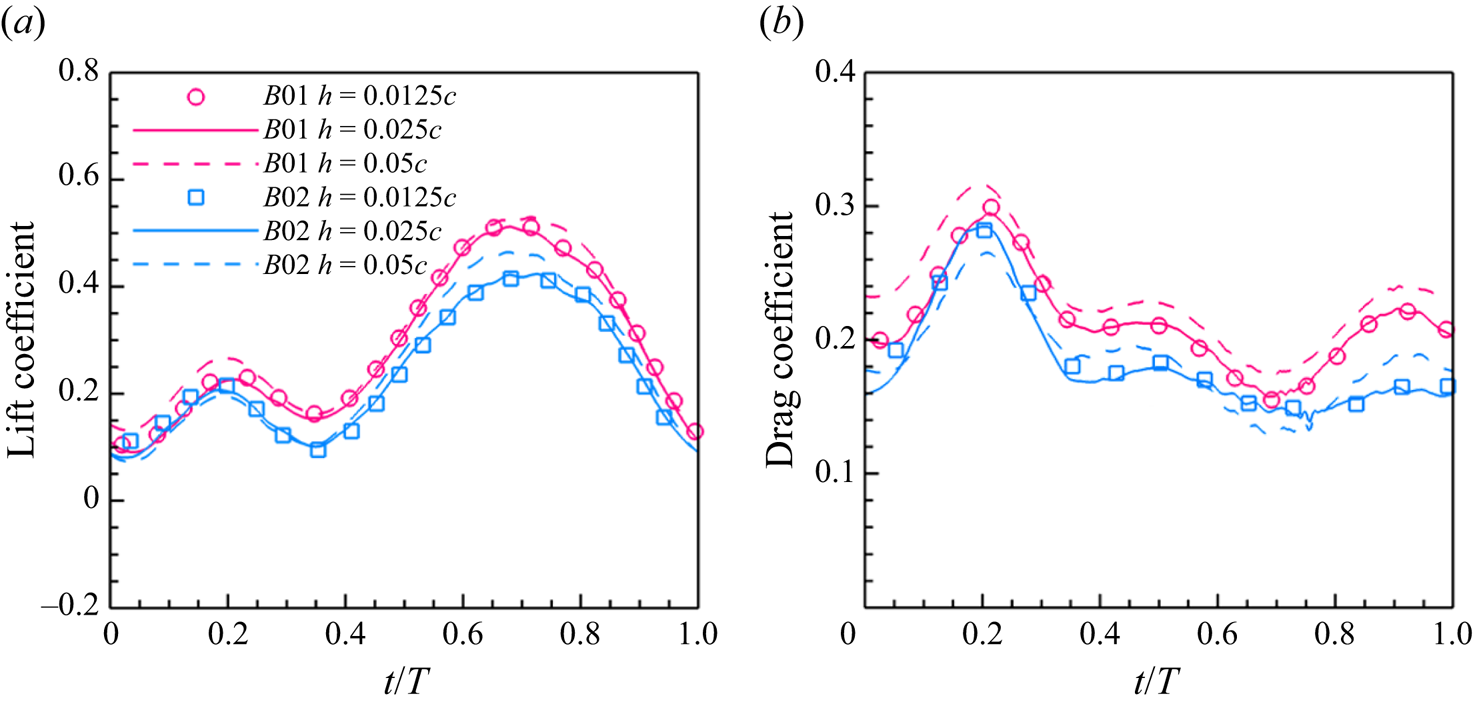
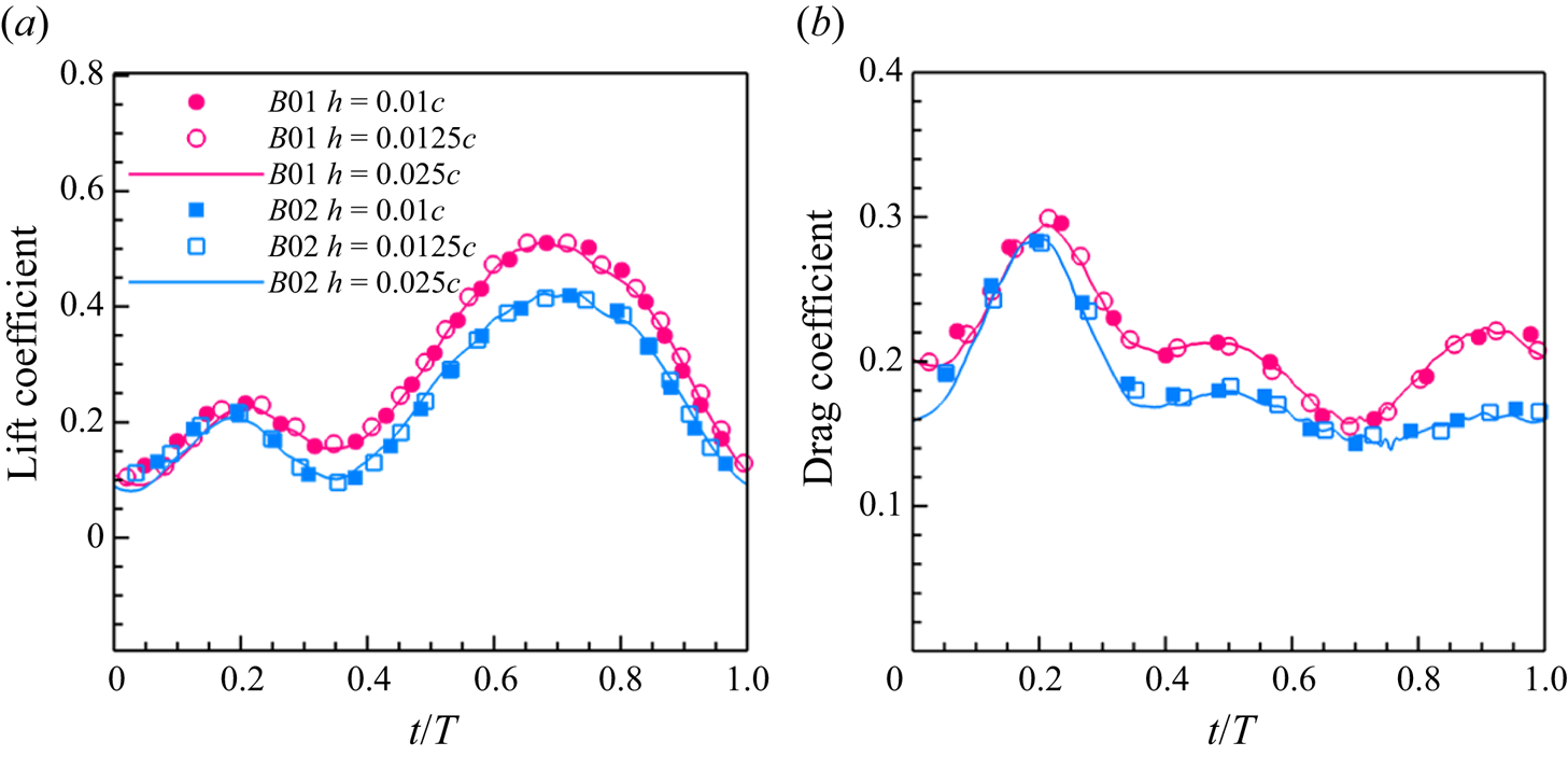
 ${Re }_{max}=330$. The convergence study of mesh size at this Reynolds number is reported in Appendix B.
The computational domain is a rectangular box with dimensions  $[-6c,12c]\times [-9c,9c]\times [-9c,9c]$ in the streamwise, spanwise and vertical directions, respectively. The mesh near the wall is locally refined, and the minimum mesh size of the Eulerian mesh,
 $h=c/40$, is used to match the average mesh size of the butterfly-inspired flapping wing. The thickness of the wing is zero on the Lagrangian mesh, since the flapping wing model consists of a single layer of Lagrangian mesh. The zero-thickness wing is taken in accordance with the previous work using the immersed boundary method, such as that of Liu, Dong & Li (Reference Liu, Dong and Li2016).
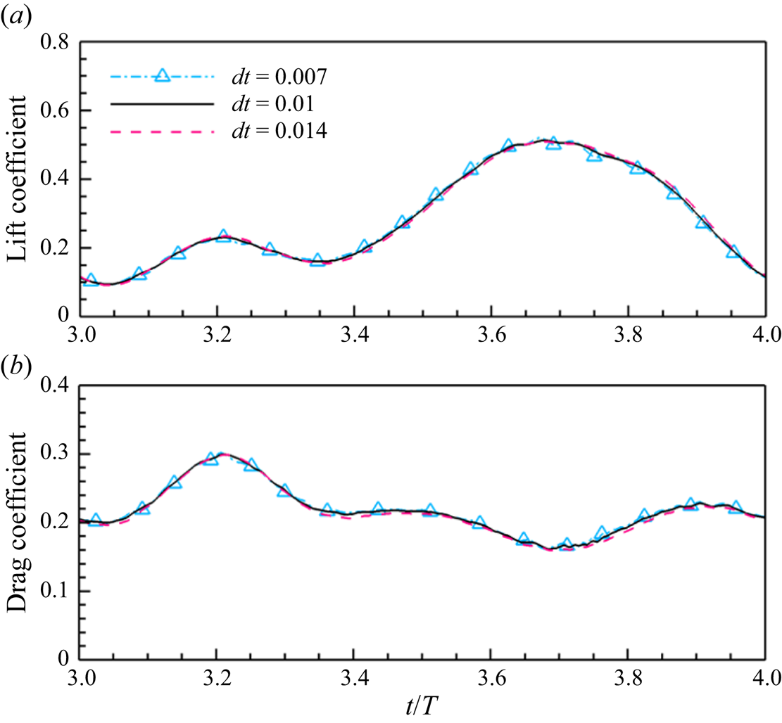
The mesh size has been validated by multiple biological propulsion cases, and it has been proved that the mesh resolution and computational domain size have little effect on the time-averaged lift and drag at the Reynolds number investigated in this work (Wang et al. Reference Wang, Zhang, He and Liu2014; Wang, He & Zhang Reference Wang, He and Zhang2015a; Tong et al. Reference Tong, Yang and Wang2021; Wang et al. Reference Wang, Liu, Xu and Wang2022). A convergence study of the spatial resolution and temporal resolution for the present study is also reported in Appendix B. The boundary conditions of the computational domain include a uniform inflow at the inlet, a free convective condition at the outlet, a no-slip boundary condition on the surface of the flapping wing and free-slip boundary conditions on the remaining four boundaries. In the present study, the Strouhal number  $St$ is given by
 \begin{equation} St=\frac{fA_{m}}{U_\infty}, \end{equation}
where  $A_{m}$ is the maximum magnitude of the wingtip motion of the imitation butterfly flapping wing model, which can be calculated as
 $A_{m}=2|AF|\sin (\varPsi _{fm})$. We refer to the butterfly motion given by Le Roy et al. (Reference Le Roy, Debat and Llaurens2019b) and Johansson & Henningsson (Reference Johansson and Henningsson2021) and set the Strouhal number in this work to
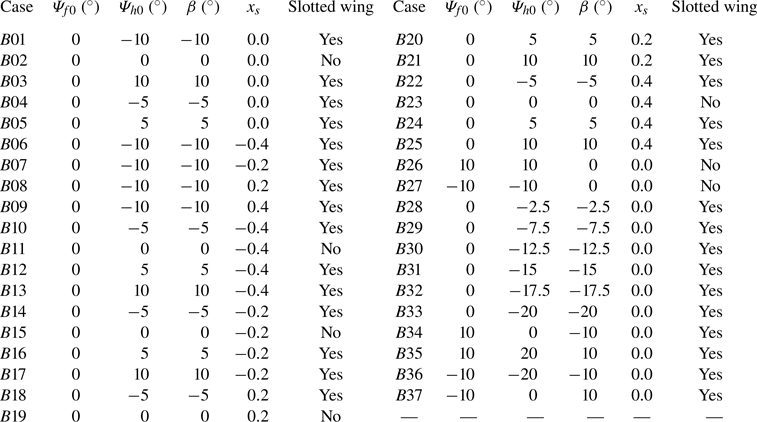
 $St= 0.3$ to make it close to that in actual flight. The case identifiers for all the cases considered in this paper and the corresponding values of the wing parameters are shown in table 2.
Cases considered in this paper. Those with dihedral angle  $\beta = 0^\circ$ are regarded as wings without a slot.

3. Results and discussion
3.1. Effects of dihedral angle and slot position on aerodynamic performance
To illustrate comprehensively the effect of a slot between the forewing and hindwing on the aerodynamic performance of the butterfly-inspired flapping wing model, simulation results for cases with different values of the slot parameters will be presented. The aerodynamic coefficients, namely the lift coefficients of the total wing ( $C_{L}$) and the drag coefficient of the total wing (
 $C_{D}$), are given by
 \begin{gather} C_{L} = \frac{L}{\dfrac{1}{2}\rho U^2_{\infty} S}, \end{gather}
 \begin{gather}C_{D} = \frac{D}{\dfrac{1}{2}\rho U^2_{\infty} S}, \end{gather}
where  $L$ and
 $D$ are the lift of the total wing and the drag of the total wing, respectively. Here,
 $S$ is the area of the total wing, and
 $\rho$ is the fluid density. The lift and drag of the total wing are given by (Wang & Zhang Reference Wang and Zhang2011)
 \begin{gather} L ={-}\sum_{j=1}^{M} {F}_z(\boldsymbol{X}_j){\Delta s} ={-}\sum_{\boldsymbol{x}} {f}_z(\boldsymbol{x}){h^3} , \end{gather}
 \begin{gather}D ={-}\sum_{j=1}^{M} {F}_x(\boldsymbol{X}_j){\Delta s} ={-}\sum_{\boldsymbol{x}} {f}_x(\boldsymbol{x}){h^3}, \end{gather}
where  ${F}_z$ and
 ${F}_x$ are the Lagrangian forces in the vertical and streamwise direction, respectively. Here,
 ${f}_z$ and
 ${f}_x$ are body forces in the vertical and streamwise directions at the Eulerian mesh, respectively,
 $M$ is the number of the Lagrangian points,
 $\boldsymbol {X}_j$ denotes the position vector of the Lagrangian point
 $j$,
 $\Delta s$ is the surface area associated with each Lagrangian point and
 $h$ is the minimum size of the Eulerian mesh. The time-averaged values of these coefficients are calculated as follows:
 \begin{gather} \bar{C}_L = \frac{\displaystyle\int_{(N-1)T}^{NT} C_{L} \,\mathrm{d}t}{T}, \end{gather}
 \begin{gather}\bar{C}_D = \frac{\displaystyle\int_{(N-1)T}^{NT} C_{D} \,\mathrm{d}t}{T}, \end{gather}
where  $N$ indicates for the
 $N$th flapping period and
 $T$ is the dimensionless flapping period of the model;
 $N=4$ in the present work.
In figure 3(a,b), it can be seen that the lift coefficients for the cases with positive dihedral angle are lower than those for the cases with negative dihedral angle. A positive dihedral angle corresponds to the hindwing being higher than the forewing, and a negative dihedral angle corresponds to the hindwing being lower than the forewing. For the lift coefficients of the total wing (figure 3a,b), the peak during the downstroke is gradually enhanced as the dihedral angle  $\beta$ decreases. In figure 3(b), the peak lift coefficient for the case with dihedral angle
 $\beta = -10^{\circ }$ is increased by 21 % compared with the case without a slot (dihedral angle
 $\beta = 0^{\circ }$), and the peak lift coefficient for the case with dihedral angle
 $\beta = 10^{\circ }$ is decreased by 20 % compared with the case without a slot (dihedral angle
 $\beta = 0^{\circ }$). Meanwhile, it can be noticed that the lift coefficient curves of the two cases with dihedral angle
 $\beta = -10^{\circ }$ and
 $\beta = -15^{\circ }$ are close to each other. In figure 3(b), the peak lift coefficient difference between cases
 $B31$ (
 $\beta = -15^{\circ }$) and
 $B01$ (
 $\beta = -10^{\circ }$) is smaller compared with the peak lift coefficient difference between cases
 $B01$ (
 $\beta = -10^{\circ }$) and
 $B04$ (
 $\beta = -5^{\circ }$). In the above simulations, the slot position in all these cases is kept at
 $x_{s} = 0.0$. This means that the chord lengths of the forewing and hindwing are the same, as are their wing areas.
Lift coefficient curves of cases with different dihedral angles and the same position of the slot at  $x=0.0$. Case
 $B02$ (
 $\beta =0^{\circ }$) is the case without a slot. (a) Lift coefficients of total wing
 $C_{L}$. (b) Peaks of lift coefficients for cases with different dihedral angles.

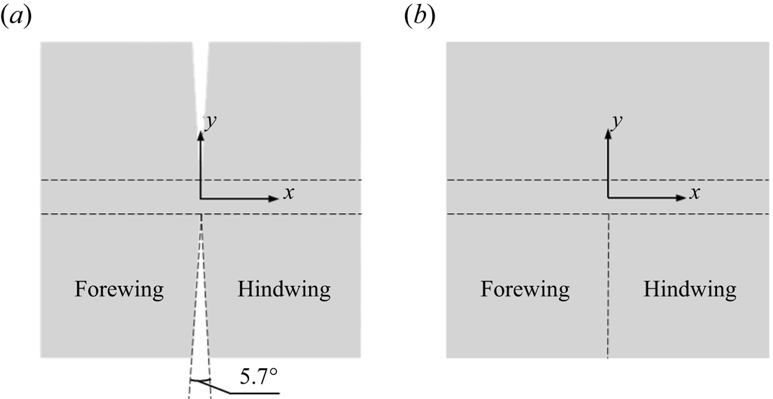
To investigate the effects of the area ratio of forewing to hindwing on the aerodynamic forces, the slot position  $x_{s}$ is set to
 $-0.4$,
 $-0.2$, 0.0, 0.2 and 0.4, as shown in figure 4(a). When the slot position
 $x_{s}$ changes from
 $-0.4$ to 0.4, the area ratio of the forewing to the hindwing changes from 0.1 to 9.0. When the slot position is
 $x_{s} = -0.4$ or
 $-0.2$, the area of the forewing is less than that of the hindwing. When the slot position is
 $x_{s} = 0.4$ or
 $0.2$, the area of the forewing is greater than that of the hindwing. From figure 4(b), we can see that the change in lift due to changing the slot position is not as significant as the change in lift due to changing the dihedral angle. The time-averaged lift coefficients for the cases
 $x_{s}=0.2$ and
 $x_{s}=0.4$ with larger forewings are close to those for the case
 $x_{s}=0$, and the time-averaged lift coefficients for the cases
 $x_{s}=-0.2$ and
 $x_{s}=-0.4$ with smaller forewings are reduced compared with the case
 $x_{s}=0$. The maximum reduction is less than 9 %.
(a) Schematic of the slotted wing with different slot positions  $x_{s}$. Here,
 $x_{s}$ denotes the
 $x$-direction position of the slot. The flapping wing model shown corresponds to slot position
 $x_{s}=0.0$, and the other areas marked on the wing by dashed lines represent slots with different slot positions
 $x_{s}$. (b) Lift coefficient curves of the total wing with different slot positions
 $x_{s}$ and the same dihedral angle
 $\beta =-10^{\circ }$.

To obtain a comprehensive view of the effects of slot position and dihedral angle on aerodynamic performance, cases with the different parameters shown in table 2 are simulated. In figure 5(a), the five curves represent five different slot positions, with the points on each curve representing the time-averaged lift coefficients  $\bar {C}_L$ corresponding to different dihedral angles. When the dihedral angle
 $\beta < 0^{\circ }$, a slot located at the front of the model causes a decrease less than 9 % in the time-averaged lift compared with the case with slot position
 $x_{s}=0.0$, as shown by the slot position
 $x_{s}=-0.4$ and
 $-0.2$ curves in figure 5(a), whereas a slot located at the rear of the model (
 $x_{s}=0.4$,
 $0.2$) will have little effect on the lift. When the dihedral angle
 $\beta < -10^{\circ }$, the time-averaged lift coefficient of the model starts to show a stable trend as the dihedral angle
 $\beta$ decreases. From figure 5(b), we can see that, when dihedral angle
 $\beta < -12.5^{\circ }$, the lift-to-drag ratio of the model starts to decay, and the continuously decreasing
 $\beta$ enhances the drag and cannot further enhance the lift.
(a) Curves of average lift coefficient vs dihedral angle  $\beta$ for cases with different slot positions
 $x_{s}$. (b) Curves of lift-to-drag ratio vs dihedral angle
 $\beta$ for cases with different slot positions
 $x_{s}$. (c) Phase diagram of lift vs lift-to-drag ratio for different cases. Each curve represents a specific slot position
 $x_{s}$. The dihedral angle gradually decreases along each curve, from left to right. The leftmost point on each curve represents the average lift coefficient and lift-to-drag ratio when dihedral angle
 $\beta = 10^{\circ }$. It can be observed that there is a sudden shift around a dihedral angle of
 $\beta = -10^{\circ }$, where the lift-to-drag ratio of the butterfly-inspired flapping wing model rapidly decreases. (d) Partial enlargement of the dashed box in (c).

In figure 5(c,d), when the dihedral angle of the model changes from  $\beta = -10^{\circ }$ to
 $-20^{\circ }$, the average lift coefficients of the model are almost the same, but the lift-to-drag ratio decreases rapidly. The large dihedral angle causes the gap of the slot near the wingtip to be sufficiently large that a leading-edge vortex forms on the hindwing. This means that the dihedral angle
 $\beta = -10^{\circ }$ represents an almost critical point for aerodynamic performance, and continuing to reduce the dihedral angle will adversely affect the aerodynamic performance of the model.
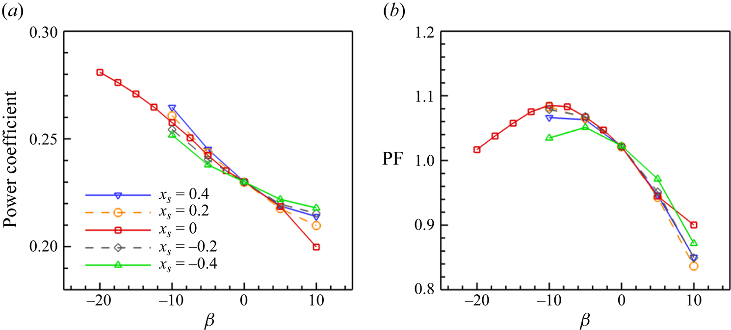
The instantaneous power expenditure of the butterfly-inspired flapping wing in the incoming velocity  $U_{\infty }$ is calculated by (3.7) according to the previous work (Wang Reference Wang2008; Lentink, Jongerius & Bradshaw Reference Lentink, Jongerius and Bradshaw2009; Shi, Xiao & Zhu Reference Shi, Xiao and Zhu2020)
 \begin{equation} P(t) = \iint_{S}-\boldsymbol{F}_{IB} (\boldsymbol{X},t)\boldsymbol{\cdot}\boldsymbol{V}(\boldsymbol{X},t)\,{\rm d}S = \iint_{S}-\boldsymbol{F}_{IB} (\boldsymbol{X},t)\boldsymbol{\cdot}\boldsymbol{V}_g (\boldsymbol{X},t)\,{\rm d}S + D(t)U_{\infty}, \end{equation}
where  $\boldsymbol {X}$ represents the position of the Lagrangian points,
 $\boldsymbol {F}_{IB} (\boldsymbol {X},t)$ is instantaneous aerodynamic force at
 $\boldsymbol {X}$ on the flapping wing,
 $\boldsymbol {V}(\boldsymbol {X},t)$ is the velocity of the flapping wing relative to the uniform upstream flow at infinity,
 $\boldsymbol {V}_g (\boldsymbol {X},t)$ is the velocity of the flapping wing relative to the centre of the model and
 $D(t)$ is the instantaneous total drag force on the flapping wing. The time-averaged power coefficient is then obtained according to the following equation (Shi et al. Reference Shi, Xiao and Zhu2020):
 \begin{equation} \bar{C}_P = \int_{(N-1)T}^{NT} \frac{P(t)}{1/2 {\rho} U_{\infty}^3 S} \,{\rm d}t. \end{equation}
We have also examined the performance of the model using the power factor ( ${\rm PF}$) to measure the lift production per unit aerodynamic power (Wang Reference Wang2008; Huang et al. Reference Huang, Bhat, Yeo, Young, Lai, Tian and Ravi2023). The equation for the power factor calculation is given as follows:
 \begin{equation} {\rm PF} = \frac{\bar{C}_L}{\bar{C}_P}. \end{equation}
In figure 6, the time-averaged power coefficient and the variation of power factor ( ${\rm PF}$) with different dihedral angles are shown. It can be noticed that the time-averaged power coefficient decreases with increasing dihedral angle (from left to right), because increasing dihedral angle (from left to right) causes the total drag and lift of the butterfly-inspired flapping wing to decrease. For the power factor, its tendency is generally in agreement with that of the lift-to-drag ratio in figure 5(c). In figure 6, the power factor approaches a maximum value at dihedral angle
 $\beta =-10^{\circ }$ for the cases with
 $x_{s}=0$, which is consistent with the results in figure 5(c).
(a) Curves of average power coefficient vs dihedral angle  $\beta$ for cases with different slot positions
 $x_{s}$. (b) Curves of power factor (
 ${\rm PF}$) vs dihedral angle
 $\beta$ for cases with different slot positions
 $x_{s}$.

3.2. Aerodynamic forces of butterfly-inspired flapping wing with and without a slot
Compared with the butterfly-inspired flapping wing without a slot, the non-zero dihedral angle  $\beta$ causes different mean elevation angles between the forewing and hindwing. Here, we simulate cases without a slot at different mean elevation angles to identify their roles in aerodynamic forces. Simulation results for cases
 $B26$ and
 $B27$ in table 2 are presented and contrasted with the baseline case
 $B02$. For cases
 $B26$ and
 $B27$, the mean elevation angle of the forewing
 $\varPsi _{f0}$ is equal to that of the hindwing
 $\varPsi _{h0}$, indicating that the forewing and hindwing are in the same plane.
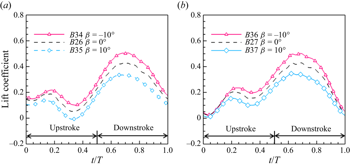
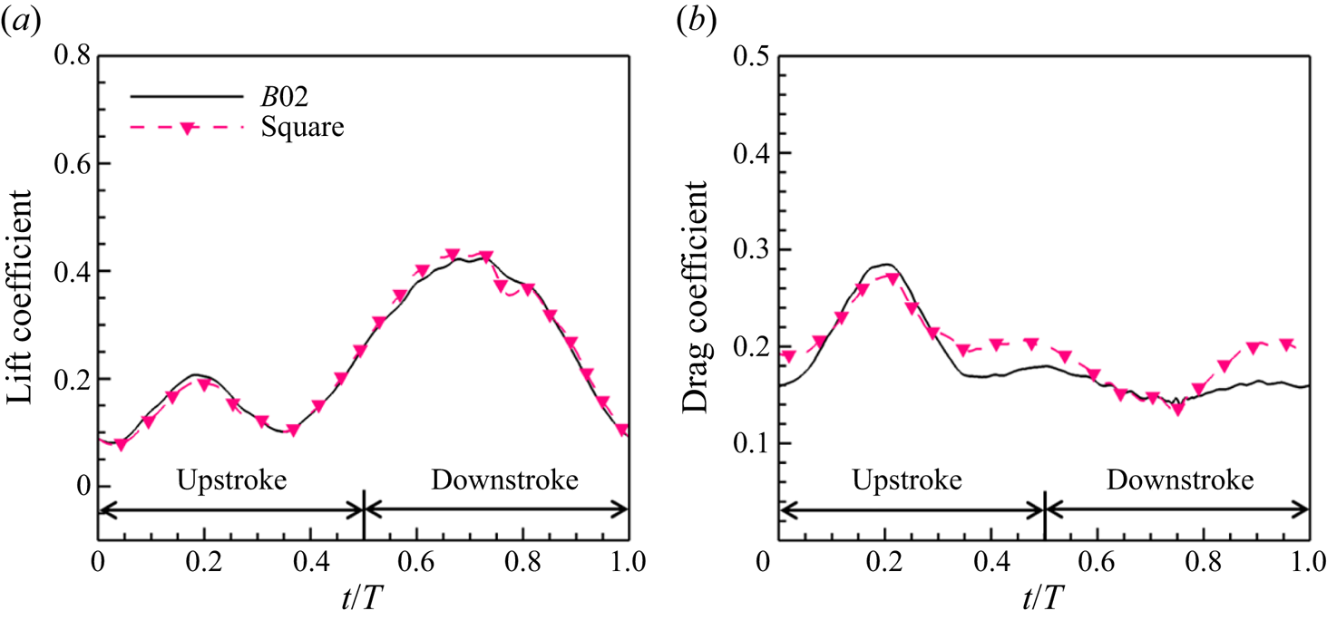
Figure 7 shows the aerodynamic forces for the cases with the mean elevation angles of the butterfly-inspired flapping wing model without a slot at  $10^{\circ }$,
 $-10^{\circ }$ and
 $0^{\circ }$. It can be observed that the lift coefficients of the total wing for these three cases exhibit peaks during the upstroke and downstroke, with the peaks for all three cases being close to each other. The lift coefficient peaks during the downstroke of the cases with
 $\varPsi _0 = 10^{\circ }$ and
 $\varPsi _0 = -10^{\circ }$ change by less than
 $1\,\%$ relative to the case with
 $\varPsi _0 = 0^{\circ }$. Nevertheless, there is a significant difference between the three cases at the minimum lift coefficients in figure 7(a). The minimum lift coefficient for the case with
 $\varPsi _0 = 10^{\circ }$ is 35 % lower than that for the case with
 $\varPsi _0 = 0^{\circ }$, and the minimum lift coefficient for the case with
 $\varPsi _0 = -10^{\circ }$ is
 $68\,\%$ lower than that for the case with
 $\varPsi _0 = 0^{\circ }$ at approximately
 $t/T = 0.35$.
Lift and drag coefficients of butterfly-inspired flapping wing without a slot (dihedral angle  $\beta = 0^\circ$). The mean values of the elevation angles of the forewing and hindwing satisfy
 $\varPsi _{f0} = \varPsi _{h0} = \varPsi _0$. (a) Lift coefficients of total wing. For all three cases, the lift coefficients exhibit extreme values during both the upstroke and downstroke. (b) Drag coefficients of total wing. These exhibit a a peak during the upstroke and change slightly during the downstroke. The solid orange line shows the angle of attack of the model, with values given on the right vertical axis.

It can be observed from figure 7(b) that the drag coefficients for all three cases exhibit a peak during the upstroke. This is caused by the enhancement of the angle of attack of the model at this stage. Along with the decrease in the angle of attack, the drag coefficients gradually decrease and become stable during the downstroke.
The changes in the mean elevation angle have little effect on the aerodynamic performance of the case without a slot. The time-averaged aerodynamic coefficients for these cases are shown in table 3. We can see that a change in mean value of the elevation angle significantly affects the minima of the model's lift coefficients, but has an essentially neglectable effect on the time-averaged lift coefficients of the total wing in table 3. When the mean value of the elevation angle is changed from  $-10^{\circ }$ to
 $10^{\circ }$, the lift coefficient of the total wing is only reduced by
 $1.7\,\%$, and the time-averaged drag coefficient remains almost constant.
Time-averaged aerodynamic coefficients for models without a slot.

In the present work, the slot generated by the dihedral angle  $\beta$ in (2.4) is considerably narrow in contrast to the case of a dragonfly's forewing and hindwing, which are approximately a chord length apart (Wang & Russell Reference Wang and Russell2007). During a wingbeat, the height difference between the wingtips of
 $AB$ (forewing) and
 $CD$ (hindwing) for the case with dihedral angle
 $\beta = 0^{\circ }$ is 0, and the height difference between the wingtips of
 $AB$ and
 $CD$ for the cases with dihedral angle
 $\beta = 10^{\circ }$ and
 $\beta = -10^{\circ }$ is only
 $0.08c$. This means that the maximum gap of the slotted wing is less than 8 % of the chord length.
From table 4, we can see that, even though the wing slot is so narrow, there has been a significant change in the lift coefficient of the total wing with a slot. The time-averaged lift coefficients  $\bar {C}_{L}$ of the case with dihedral angle
 $\beta = -10^{\circ }$ is increased by 20 % compared with the case without a slot (dihedral angle
 $\beta = 0^{\circ }$), and
 $\bar {C}_{L}$ of the case with dihedral angle
 $\beta = 10^{\circ }$ is decreased by 22 % compared with the case without a slot. Through the time-averaged lift coefficients presented in tables 3, 4 and Appendix C, we can identify that changing the dihedral angle, rather than changing the mean value of the elevation angle, is responsible for the time-averaged lift enhancement.
Time-averaged aerodynamic coefficients for cases  $B01$ and
 $B03$ with a slot and case
 $B02$ without a slot.

A change in the dihedral angle  $\beta$ has a remarkable effect not only on the lift of the model, but also on the drag. From table 4, it can be seen that the time-averaged drag for the case with a dihedral angle
 $\beta = -10^{\circ }$ is increased by 18 % compared with the case without a slot, and the time-averaged drag for the case with a dihedral angle
 $\beta = 10^{\circ }$ is decreased by 8 % compared with the case without a slot. Even with the increase in drag, the lift enhancement generated by the negative dihedral angle is sufficient to improve the lift-to-drag ratio in figure 5(b), when the dihedral angle
 $\beta >-10^{\circ }$. When the dihedral angle
 $\beta < 10^{\circ }$, the lift of the model remains almost constant, and the drag continues to increase, resulting in the lift-to-drag ratio decreasing.
It is important to realize that the cases with dihedral angle  $\beta = -10^{\circ }$ and
 $\beta = 10^{\circ }$ differ significantly in their aerodynamic performance, although they both feature a wing slot. The forewing–hindwing interactions can significantly enhance the lift if the slot is properly configured. However, it is noticed that a slot in the flapping wing model does not always enhance the aerodynamic performance of the model, and may even have a negative effect. The above results indicate that the case with a slot possesses a higher lift-to-drag ratio and power factor compared with the case without a slot, which is closely related to the enhancement of lift. In the next subsection, we choose the unsteady lift as the focus. On the basis of the present aerodynamic data, we can see that it is worth discussing and analysing how the dihedral angle
 $\beta$, which is small compared with the elevation amplitude, causes such a significant lift change.
3.3. Vortex structures
The vortex structures around the flapping wing are investigated to understand the effects of the dihedral angle on the interaction between the forewing and hindwing. Figures 8(a–c) and 8(d–f) show the vortex patterns during the upstroke for the cases with dihedral angle  $\beta = -10^{\circ }$ and
 $\beta = 0^{\circ }$, respectively, at the moments
 $t/T = 0.1$,
 $0.3$ and
 $0.4$. In these figures, the leading-edge vortex (LEV) and tip vortex (TV) in the flow field are identified.
The flapping wing position and the flow around it. The isosurface of the  $Q$-criterion during the upstroke for butterfly-inspired flapping wing models with (a–c) the dihedral angle
 $\beta = -10^{\circ }$ and (d–f) the dihedral angle
 $\beta = 0^{\circ }$ (the case without a slot): grey,
 $Q=0.75$; cyan,
 $Q=6$. A snapshot of the wing model at the corresponding time is shown at the lower left of each panel. (g) The spanwise vorticity distribution
 $\omega _y$ at the
 $y = -0.45$ spanwise slice for
 $\beta =-10^{\circ }$. (h) The spanwise vorticity distribution
 $\omega _y$ at the
 $y = -0.45$ spanwise slice for
 $\beta =0^{\circ }$. Subscripts DS and US stand for downstroke and upstroke, respectively,
 $N$ denotes the vortex pattern generated by the
 $N$th flapping period and
 $N-1$ the vortex pattern generated by the
 $(N-1)$th flapping period. The grey vortex surface reflects the wake features and the cyan vortex surface the vortex distribution features near the wing (colour online). The main vortex patterns during the upstroke are leading-edge vortex shedding in the previous cycle, tip vortices of the forewing and hindwing and a new leading-edge vortex generated along with increasing angle of attack.

As can be seen in figure 8(a,d), the LEV generated during the downstroke of the ( $N-1$)th period is separating at the initial stage of the upstroke of the
 $N$th period. Owing to the upstroke motion of the wing, most of the vortices at this stage are distributed on the ventral side of the wing, and the dorsal vortices are relatively sparse. During the upstroke (figure 8b,c), with gradually increasing angle of attack, a new LEV (
 $\text {LEV}_{US,N}$) begins to be generated.
In figure 8(b,c), it can be seen that the wingtip vortices of the forewing and hindwing are at different heights, owing to the presence of the dihedral angle, and a strong shear flow is generated at the slot location, as shown in figure 8(g). The wingtip vortices of the wing without a slot are smoothly and uniformly distributed along the forewing and hindwing wingtips, as shown in figure 8(e,f,h).
During the upstroke, the cases with dihedral angle  $\beta = -10^{\circ }$ and
 $\beta = 0^{\circ }$ have similar LEVs, differing only in strength. To clarify the difference in strength, we computed the circulation associated with the LEV. The difference in strength can be represented by the differences between the circulations. In the present work, we use the
 $Q > 6$ isosurface as a reference for the boundary of the LEV (Eldredge & Jones Reference Eldredge and Jones2019). The integration of the LEVs is performed during the upstroke within the region of
 $Q > 6$ at 75 % wingspan slice. The
 $\text {LEV}_{US,N}$ circulation at 75 % wingspan slice is shown in table 5 for the case with a slot (
 $\beta = -10^{\circ }$) and the case without a slot (
 $\beta = 0^{\circ }$) during the upstroke. From the results of integration at multiple instants, it can be seen that the slot enhances the strength of the LEVs.
The circulations of LEVs within the region of  $Q > 6$ during the upstroke for the case
 $B01$ with a slot and case
 $B02$ without a slot at the 75 % wingspan slice. The region where the LEVs are integrated is shown in figure 26 of Appendix E.

In figure 9, the LEV, TV and trailing-edge vortex (TEV) induced by the downstroke are indicated. At the beginning of the downstroke, the angle of attack of the model starts to decrease, as a result of which the LEV  $\text {LEV}_{US,N}$ formed during the upstroke starts to be shed. Meanwhile, a new LEV
 $\text {LEV}_{DS,N}$ starts to be generated owing to the downward flapping motion of the wing. Within one wingbeat, the leading edge of the wing will generate two LEVs owing to the increasing angle of attack and the flapping motion, namely
 $\text {LEV}_{US,N}$ and
 $\text {LEV}_{DS,N}$, respectively.
The flapping wing position and the flow around it. The isosurface of the  $Q$-criterion during the downstroke for the butterfly-inspired flapping wing models with (a–c) the dihedral angle
 $\beta = -10^{\circ }$ and (d–f) the dihedral angle
 $\beta = 0^{\circ }$ (the case without a slot): grey,
 $Q=0.75$; cyan,
 $Q=6$. A snapshot of the wing model at the corresponding time is shown at the lower left of each panel. (g) The spanwise vorticity distribution
 $\omega _y$ at the
 $y = -0.45$ spanwise slice for
 $\beta =-10^{\circ }$. (h) The spanwise vorticity distribution
 $\omega _y$ at the
 $y = -0.45$ spanwise slice for
 $\beta =0^{\circ }$. Subscripts DS and US stand for downstroke and upstroke, respectively,
 $N$ denotes the vortex pattern generated by the
 $N$th flapping period. The grey vortex surface reflects the wake features and the cyan vortex surface the vortex distribution features near the wing (colour online). The main vortex patterns during the downstroke are a fully developed TV, a LEV induced by the flapping motion and a trailing-edge vortex.

As shown in table 5, the integration of the LEVs is performed at the 75 % wingspan slice within the region of  $Q > 6$ during the downstroke. The
 $\text {LEV}_{{DS,N}}$ circulation at the 75 % wingspan slice is shown in table 6 for the case with a slot (
 $\beta = -10^{\circ }$) and the case without a slot (
 $\beta = 0^{\circ }$) during the downstroke. From the results of integration at multiple instants, it can be seen that the slot also enhances the strength of the LEVs generated during the downstroke.
The circulations of LEVs within the region of  $Q > 6$ during the downstroke for the case
 $B01$ with a slot and case
 $B02$ without a slot at the 75 % wingspan slice. The region where the LEVs are integrated is shown in figure 27 of Appendix E.

As shown in figure 9(c), the TV of the forewing  $\text {TV}_{f}$ with dihedral angle
 $\beta = -10^{\circ }$ is fully developed during the downstroke, and
 $\text {TV}_{f}$ begins to be shed at the end of the downstroke. The detached TV of the forewing
 $\text {TV}_{f}$, as shown in figure 9(c,g), has a stronger shear strength than the detached TV in figure 9(f,h).
In general, the patterns of LEV and TEV generated in the cases with dihedral angles  $\beta = -10^{\circ }$ and
 $\beta = 0^{\circ }$ are similar during the downstroke, but the shear strength of the vortices is enhanced owing to the presence of the slot caused by a non-zero dihedral angle
 $\beta$. The spatial distribution of the wingtip vortices in the case with a slot is obviously different from that in the absence of a slot, because the non-zero dihedral angle results in the forewing being in a different plane from the hindwing.
3.4. Vortex lift
To identify the vortex structures responsible for the change in lift due to the dihedral angle  $\beta$, we use (2.6) to decompose the lift of the butterfly-inspired flapping wing model into vortex lift and inertial force. From figure 10(a), it can be seen that the inertial force peak in the case with dihedral angle
 $\beta = -10^{\circ }$ is smaller than that in the case with dihedral angle
 $\beta = 0^{\circ }$ (case
 $B02$
 $\beta =0^{\circ }$ is the case without a slot), but the vortex lift in the case with dihedral angle
 $\beta = -10^{\circ }$ is larger than that in the case with dihedral angle
 $\beta = 0^{\circ }$ over the whole period. In fact, the period averages of the inertial force and vortex lift in the case with dihedral angle
 $\beta = -10^{\circ }$ are improved compared with the case with dihedral angle
 $\beta = 0^{\circ }$. The vortex lift increment accounts for 70 % of the total lift increment and the inertial force increment accounts for 30 % of the total lift increment. Therefore, we can determine that the increment in lift for the case with a negative dihedral angle is dominated by the increment in vortex lift. On decomposing lift into inertial force and vortex lift, it becomes apparent that it is the variation in vortex lift that predominantly dictates the changes in total lift for cases with different dihedral angles.
(a) Vortex lift (‘lamb’) and inertial force (‘acc’) coefficient curves for dihedral angles  $\beta = -10^{\circ }$ and
 $0^{\circ }$. Case
 $B02$ (
 $\beta =0^{\circ }$) is the case without a slot. The vortex lift coefficient and inertial force coefficient curves are obtained from the
 $z$ components in the first and second terms, respectively, on the right-hand side of (2.6), namely
 $\rho \int _{V_{f}} (\boldsymbol {u}\times \boldsymbol {\omega })_z \,\mathrm {d}V$ and
 $- \rho \int _{V_{f}} ({\partial \boldsymbol {u}}/{\partial t})_z \,\mathrm {d}V$. The dashed lines represents the inertial force in the
 $z$ direction and the dot-dashed lines the vortex lift force. (b) To analyse the effects of the combination of streamwise velocity and spanwise vorticity and the combination of spanwise velocity and streamwise vorticity on vortex lift, curves of
 $\rho \int _{V_{f}} u \omega _y \,\mathrm {d}V$ and
 $\rho \int _{V_{f}} (-v \omega _x) \,\mathrm {d}V$ are plotted for cases with dihedral angles
 $\beta = -10^{\circ }$ and
 $0\,^{\circ }$. Here,
 $u \omega _y$ and
 $-v \omega _x$ are the components of the Lamb vector in the direction of lift and reflect the respective effects of the combination of streamwise velocity and spanwise vorticity and the combination of spanwise velocity and streamwise vorticity on the vortex lift.

It is necessary to decompose the vortex lift to figure out the relationship between the enhancement of vortex lift and the forewing–hindwing interaction. The Lamb vector  $\boldsymbol {u} \times \boldsymbol {\omega }$ in the lift direction can be expressed as follows:
 \begin{equation} (\boldsymbol{u} \times \boldsymbol{\omega})_z = u\omega_y - v\omega_x, \end{equation}
where  $u$ and
 $v$ are the velocity components in the
 $x$ (streamwise) and
 $y$ (spanwise) directions, respectively, and
 $\omega _x$ and
 ${\omega }_y$ are the
 $x$ and
 $y$ components of the vorticity
 $\boldsymbol {\omega }$. The first term on the right-hand side of (3.10),
 $u{\omega }_y$, represents the effects of the combination of streamwise velocity and spanwise vorticity on vortex lift, while the second term,
 $-v{\omega }_x$, represents the effect of the combination of spanwise velocity and streamwise vorticity. Thus, the reasons for changes in vortex lift can be determined by investigating the combination of streamwise velocity and spanwise vorticity and the combination of spanwise velocity and streamwise vorticity.
In figure 10(b), we can see difference in the vortex lift component  $u{\omega }_y$ between the cases with
 $\beta =-10^{\circ }$, and
 $\beta =0^{\circ }$ during the downstroke, and so we choose two moments
 $t/T=0.6$ and
 $0.8$ (figures 11 and 12, respectively) to analyse the features of the combination of streamwise velocity and spanwise vorticity for the cases with dihedral angles
 $\beta = -10^{\circ }$ and
 $\beta = 0^{\circ }$. The relevant discussion is presented in § 3.4.1. We can see that, although the vortex lift term
 $-v{\omega }_x$ representing the combination of spanwise velocity and streamwise vorticity accounts for a relatively small part of the vortex lift, there is still a meaningful difference between the case with dihedral angle
 $\beta = -10^{\circ }$ and that without a slot (dihedral angle
 $\beta = 0^{\circ }$) in
 $t/T\in [0.35, 0.55]$. Therefore, we choose the moments
 $t/T=0.4$ and
 $t/T=0.5$ (figures 13–17) to analyse the features of the combination of spanwise velocity and streamwise vorticity for the cases with
 $\beta =-10^{\circ }$ and
 $\beta =0^{\circ }$.
Contours of streamwise velocity  $u$ (a,b), spanwise vorticity
 $\omega _y$ (c,d) and vortex lift component
 $u\omega _y$ (e,f) for the spanwise slices at 75 %, 50 %, 25 % and 0 % wingspan at
 $t/T=0.6$: (a,c,e) case
 $B01$ with dihedral angle
 $\beta = -10^{\circ }$; (b,d,f) case
 $B02$ with dihedral angle
 $\beta = 0^{\circ }$ (the case without a slot). (c,d) The white isolines represent
 $Q = 6$.

Contours of streamwise velocity  $u$ (a,b), spanwise vorticity
 $\omega _y$ (c,d) and vortex lift component
 $u\omega _y$ (e,f) for the spanwise slices at 75 %, 50 %, 25 % and 0 % wingspan at
 $t/T=0.8$: (a,c,e) case
 $B01$ with dihedral angle
 $\beta = -10^{\circ }$; (b,d,f) case
 $B02$ with dihedral angle
 $\beta = 0^{\circ }$ (the case without a slot). (c,d) The white isolines represent
 $Q = 6$.

3.4.1. Effect of combination of streamwise velocity and spanwise vorticity on vortex lift
The distributions of streamwise velocity and spanwise vorticity at  $t/T=0.6$ and
 $0.8$ are analysed to figure out the role of the vortex dynamics in the forewing–hindwing interaction. At
 $t/T = 0.6$ the initial stage of the downstroke, despite the vortex lift reaching nearly its minimum value, a ten-degree change in the dihedral angle still results in a remarkable variation in the combination component
 $u\omega _y$ of the vortex lift at this stage, as shown in figure 10(b).
In figure 11, for analysing the difference in the combination of streamwise velocity and spanwise vorticity between the cases with dihedral angles  $\beta = -10^{\circ }$ (figure 11a,c,e) and
 $\beta = 0^{\circ }$ (figure 11b,d,f), we present slices at different spanwise positions at
 $t/T=0.6$. The streamwise velocity
 $u$, spanwise vorticity
 $\omega _y$ and combination component
 $u\omega _y$ of the vortex lift are shown. From figure 11, the effects of a slot on the flow mechanism can be analysed by comparison with the case with dihedral angle
 $\beta = 0^{\circ }$.
The slot reduces the streamwise velocity beneath the forewing. The black dashed line box in figure 11(a,b) is located beneath the forewing. The streamwise velocity distribution in the dashed line box in figure 11(a) has a larger proportion of the low velocity area than that in the dashed line box in figure 11(b). At the streamwise velocity contours of 75 %, 50 % and 25 % wingspan, the reduction in streamwise velocity beneath the forewing in the case with dihedral angle  $\beta = -10^{\circ }$ is remarkable, as can be seen by comparing the areas (yellow area) enclosed by the contour lines
 $u=0.7$ and
 $u=0.9$. This flow feature becomes more pronounced as the slice gets closer to the wingtip.
For the case with dihedral angle  $\beta = -10^{\circ }$, analysis of the
 $\omega _y$ distribution shows that the shear strength is lower beneath the forewing and higher beneath the hindwing compared with the case without a slot (dihedral angle
 $\beta = 0^{\circ }$). Since the vorticity
 $\omega _y$ at the abdominal side of the wing is negative, the reduction in the velocity
 $u$ at the abdominal side of the wing is equivalent to an increase in the
 $u\omega _y$ term of the vortex lift. Although the negative
 $u\omega _y$ decreases beneath the forewing (black dashed box), it increases beneath the hindwing owing to the negative
 $\omega _y$ distribution in the case with dihedral angle
 $\beta = -10^{\circ }$.
Therefore, it is necessary to analyse quantitatively the proportions of vortex lift on the forewing and hindwing. Equation (2.6) is used again to obtain the vortex lift acting on the forewing when the control volume is set to  $[-4c,0c]\times [-6c,6c]\times [-6c,6c]$. For the cases with dihedral angles
 $\beta = 0^{\circ }$ and
 $\beta = -10^{\circ }$ at
 $t/T=0.6$, the vortex lift coefficients of the forewing are
 $0.33$ and
 $0.41$, respectively. The vortex lift coefficient of the total wing is known, so the vortex lift coefficient of the hindwing for the cases with dihedral angles
 $\beta = 0^{\circ }$ and
 $\beta = -10^{\circ }$ at
 $t/T=0.6$ is
 $-0.18$ and
 $-0.10$, respectively. Compared with the case without a slot, the vortex lifts acting on the forewing and hindwing are both enhanced in the case with dihedral angle
 $\beta = -10^{\circ }$.
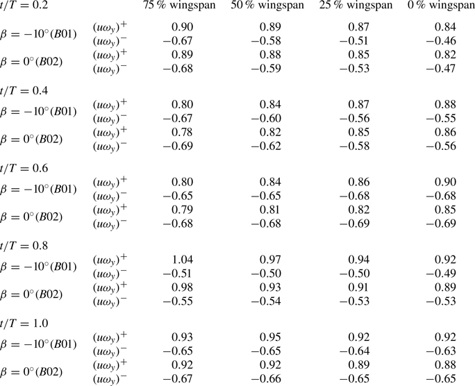
Further, we can see in table 7 the  $u\omega _y$ strength above and beneath the wing at multiple spanwise slices. In addition to the increase in
 $u\omega _y^-$ due to the deceleration beneath the forewing, we also find that, at all slices,
 $u\omega _y^+$ for the case with
 $\beta =-10^{\circ }$ is more than that for the case with
 $\beta =0^{\circ }$. This result indicates that the strength of
 $u\omega _y$ above the wing in figure 11(e) is higher than the strength of that above the wing in figure 11(f), while the difference is not obvious from these two groups of contours.
Surface integral of vortex lift component  $u\omega _y$ in multiple spanwise slices at
 $t/T=0.6$. The symbol
 $(u\omega _y)^+$ represents the integral of the positive
 $u\omega _y$ distributed above the wing, corresponding to the red region in figure 11(e,f). The symbol
 $(u\omega _y)^{-}$ represents the integral of the negative
 $u\omega _y$ distributed beneath the wing, corresponding to the blue region in figure 11(e,f). The rectangular field of integration of
 $u\omega _y$ for slices is
 $[-4c,(1+\sqrt {3})c/4]\times [-6c,6c]$ in the streamwise (x) and vertical (z) directions, respectively.

At  $t/T = 0.8$, as shown in figure 12, the LEV generated during the downstroke is almost fully developed, corresponding to the vortex lift maximum in figure 10(a). At this time in the different spanwise slices, we can observe that the hindwing with negative dihedral angle still contributes to the reduction in streamwise velocity beneath the wing. In figure 12(a,b), the velocity decrease beneath the forewing can be observed by comparing the velocity distributions in the black dashed box. At
 $t/T = 0.8$, the velocity decreasing phenomenon beneath the forewing can be observed not only at 75 % and 50 % wingspan, but also at 25 % and 0 % wingspan by comparing the lengths of the dashed arrows. The variations in the distribution of the spanwise vorticity are similar to those shown in figure 11.
The leading edge of the hindwing does not have obvious leading-edge vorticity due to the wing slot, since the gap of the slot is narrow enough, as shown in figures 11(c) and 12(c). This phenomenon is distinct from the interaction between the forewing and hindwing of a dragonfly. During the flight of a dragonfly, LEVs are present on both the forewing and hindwing owing to the long distance between these wings (Wang & Russell Reference Wang and Russell2007; Alben Reference Alben2021; Wu et al. Reference Wu, Li, Chen and Zhang2022), but the hindwing of the butterfly does not have a LEV and is always in the wake generated by the forewing.
The vortex lifts acting on the forewing and hindwing at  $t/T=0.8$ are also shown. For the cases with dihedral angles
 $\beta = 0^{\circ }$ and
 $\beta = -10^{\circ }$, the vortex lift coefficients of the forewing are
 $0.49$ and
 $0.60$, respectively, and those of the hindwing are
 $0.15$ and
 $0.13$, respectively. The decrease in the negative
 $u\omega _y$ beneath the forewing makes a remarkable contribution to the enhancement of the vortex lift acting on the forewing. Although the slot causes a slight decrease in the vortex lift on the hindwing, it still improves the vortex lift of the total wing.
As shown in table 8,  $(u\omega _y)^+$ distributed above the wing and
 $(u\omega _y)^{-}$ distributed beneath are also integrated in different spanwise slices at
 $t/T = 0.8$. While the contours of
 $u\omega _y$ for the case (
 $B01$) with
 $\beta =-10^{\circ }$ and the case (
 $B02$) with
 $\beta =0^{\circ }$ are similar in figure 12(e,f), the difference in the strengths of
 $u\omega _y$ can be quantified in table 8. In table 8, the enhancement of
 $(u\omega _y)^{-}$ occurs in multiple slices, which is different from table 7, where its enhancement only occurs in slices close to the wingtip, indicating that deceleration results in the enhancement of
 $(u\omega _y)^{-}$ at multiple locations as shown in figure 12(a,b). More results for the vortex lift component
 $u\omega _y$ at multiple instants and the detailed meaning for
 $(u\omega _y)^+$ and
 $(u\omega _y)^{-}$ can be found in Appendix E.
Surface integral of vortex lift component  $u\omega _y$ in multiple spanwise slices at
 $t/T=0.8$. The symbol
 $(u\omega _y)^+$ represents the integral of the positive
 $u\omega _y$ distributed above the wing, corresponding to the red region in figure 12(e,f). The symbol
 $(u\omega _y)^{-}$ represents the integral of the negative
 $u\omega _y$ distributed beneath the wing, corresponding to the blue region in figure 12(e,f). The rectangular field of integration of
 $u\omega _y$ for slices is
 $[-4c,(1+\sqrt {3})c/4]\times [-6c,6c]$ in the streamwise (x) and vertical (z) directions, respectively.

By analysing the white isolines ( $Q=6$) in figures 11(c,d) and 12(c,d), it is found that the LEV is longer near the wingtip than near the body. Slightly adjusting the dihedral angle (
 $-10^{\circ }\leq \beta \leq 10^{\circ }$) of the butterfly-inspired flapping wing model will not significantly affect the feature of the LEV. By analysing the streamwise velocity at
 $t/T = 0.6$ and
 $0.8$ during the downstroke, it is found that slightly adjusting the dihedral angle will affect the streamwise velocity at the abdominal side of the wing. When the hindwing is lower than the forewing, the fluid passing beneath the forewing is slowed down so that the lift acting on the forewing is enhanced. The aerodynamic mechanism implied by this phenomenon of flow is consistent with the streamwise ram effect involved in the ground effect (Jones Reference Jones2000; Lee, Han & Bae Reference Lee, Han and Bae2010; Bleischwitz, de Kat & Ganapathisubramani Reference Bleischwitz, de Kat and Ganapathisubramani2016). The difference is that, in the conventional concept of the streamwise ram effect, the ground plays the role of reducing the flow velocity, whereas in this study the hindwing plays this role. In this study, we apply the concept of the streamwise ram effect to summarize the mechanism of vortex lift enhancement caused by the combination of streamwise velocity and spanwise vorticity.
There is a stagnation region near the leading edge of the hindwing, which decreases the flow velocity and increases the static pressure (Gong, Jia & Xi Reference Gong, Jia and Xi2015). This phenomenon can be considered as a quasi-steady effect. The streamwise ram effect induced by the stagnation region can enhance the lift only when the leading edge of the hindwing is beneath the trailing edge of the forewing. For the dragonfly-inspired model, the stagnation region generated by the leading edge of the hindwing appears periodically above and beneath the trailing edge of the forewing (Broering & Lian Reference Broering and Lian2010; Gong et al. Reference Gong, Jia and Xi2015). However, this effect enhances lift during the whole flapping cycle for butterfly-inspired tandem wings in the present work, although it also increases drag.
Furthermore, this can explain why the cases with  $x_{s}=-0.4$ in figure 5(a) have lower lift than the cases
 $x_{s}=0$ when the dihedral angle
 $\beta <0$. The forewing is too small to take full advantage of the deceleration zone beneath the forewing provided by the hindwing, so the lift enhancement is not as effective as the cases with
 $x_{s}=0$.
3.4.2. Effect of combination of spanwise velocity and streamwise vorticity on vortex lift
From figure 10(b), we note that there is a difference in the effects of the combination term  $-v\omega _x$ on the vortex lift at the end of the upstroke and in the initial stage of the downstroke (
 $t/T \in [0.35,0.55]$), and so it is necessary to analyse the distribution of spanwise velocity and streamwise vorticity at
 $t/T = 0.4$ and
 $t/T = 0.5$.
To show the effect of the dihedral angle on the combination of spanwise velocity and streamwise vorticity, we present schematics of the streamwise vorticity  $\omega _x$ distribution near the wing. As can be seen in figure 13, the streamwise vorticity distributions near the leading edge are practically similar for all three cases. However, owing to the change in the relative positions of the wingtips of the forewing and hindwing, the streamwise vorticity distribution near the hindwing wingtip produces a significant difference.
Streamwise vortex distribution near the wing at  $t/T = 0.5$: (a) dihedral angle
 $\beta = -10^{\circ }$ and (b) dihedral angle
 $\beta = 0^{\circ }$ (the case without a slot). The light grey semitransparent region is the
 $\lvert \omega _x\lvert\, = 1.5$ isotropic surface, and five streamwise slices are uniformly distributed on the wing to show the streamwise vortex distribution. These streamwise slices surrounded by the
 $\omega _x$ isotropic surface clearly reflect the relative positions of the tip vortices of the forewing and hindwing.

Figure 13(a) shows the streamwise vorticity near the wing with dihedral angle  $\beta = -10^{\circ }$. The negative dihedral angle indicates that the height of the hindwing wingtip is always lower than that of the forewing wingtip during a wingbeat. It should be noted that the TV
 $\text {TV}_{f}$ of the forewing still has an effect on the combination of spanwise velocity and streamwise vorticity above the hindwing after it has shed at the interface between the forewing and hindwing.
In figure 13(b), we can observe that the forewing TV  $\text {TV}_{f}$ and hindwing TV
 $\text {TV}_{h}$ in the case with dihedral angle
 $\beta = 0^{\circ }$ are connected, and both of them attach stably to the wingtip as a complete structure and gradually decay along the streamwise direction near the hindwing. On the basis of these results, we can see that the wingtip of the hindwing being lower than that of the forewing causes the forewing TV
 $\text {TV}_{f}$ to be above the hindwing.
By analysing the streamwise vorticity distribution of the two cases, it is found that  $\text {TV}_{f}$ in the case with negative dihedral angle can shed prematurely and have an effect on the combination of spanwise velocity and streamwise vorticity near the hindwing, and there is only a hindwing TV near the hindwing wingtip in the case without a slot (figure 13b).
With completion of the comparison and analysis of the spanwise velocity and streamwise vorticity around wings with different dihedral angles  $\beta$, the distribution of the component
 $-v\omega _x$ of the vortex lift can be further discussed at
 $t/T=0.4$ and
 $t/T=0.5$. The slices at
 $x = -0.25$ in figures 14(a,d) and 16(a,d) show the spanwise velocity and streamwise vorticity near the forewing, those at
 $x = 0.0$ in figures 14(b,e) and 16(b,e) show the spanwise velocity and streamwise vorticity at the interface between the forewing and hindwing and those at
 $x = 0.3$ in figures 14(c,f) and 16(c,f) show the spanwise velocity and streamwise vorticity near the hindwing.
Distribution of the spanwise velocity and streamwise vorticity for different  $x$-position slices at
 $t/T = 0.4$: (a–c) dihedral angle
 $\beta = -10^{\circ } (B01)$; (d–f) dihedral angle
 $\beta = 0^{\circ } (B02)$. Case
 $B02$ is the case without a slot. Contour lines of the spanwise velocity and contours of the streamwise vorticity are shown. The solid and dashed contour lines represent positive and negative spanwise velocity
 $v$, respectively. In the model, the forewing is defined for
 $x \in [-0.5, 0.0)$ and the hindwing for
 $x \in (0.0, 0.5]$. The interface between the forewing and hindwing is located at
 $x = 0.0$. The three streamwise slices at
 $x = -0.25$,
 $x = 0.0$ and
 $x = 0.3$ correspond to the forewing, the forewing–hindwing interface and the hindwing, respectively.

In figure 14 ( $t/T=0.4$), the spanwise velocity
 $v$ near the total wing (both forewing and hindwing) for the case with dihedral angle
 $\beta = -10^{\circ }$ (
 $B01$) is higher than that for the case with dihedral angle
 $\beta = 0^{\circ }$ (
 $B02$). This difference can be noticed by comparing
 $v=\pm 0.18,\pm 0.24$ contour lines in figures 14(a,c), and 14(d,f). The stagnation region caused by the hindwing enhances the spanwise velocity beneath the forewing. High spanwise velocity generates strong streamwise vortices near the wingtip, and strong streamwise vortices induce high spanwise velocity above the forewing.
In order to explore the effect of higher spanwise velocity on vortex lift for the case with dihedral angle  $\beta = -10^{\circ }$ (
 $B01$), we show the distribution of
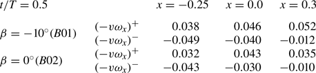
 $-v\omega _x$ in figure 15 and quantitatively calculate the contribution of
 $-v\omega _x$ to the lift coefficient by a similar calculation as in the previous section § 3.4.1. At
 $t/T=0.4$, for the case with dihedral angle
 $\beta = -10^{\circ }$ (
 $B01$), the higher spanwise velocity results in a more intense variation of
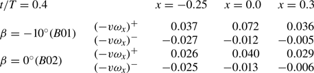
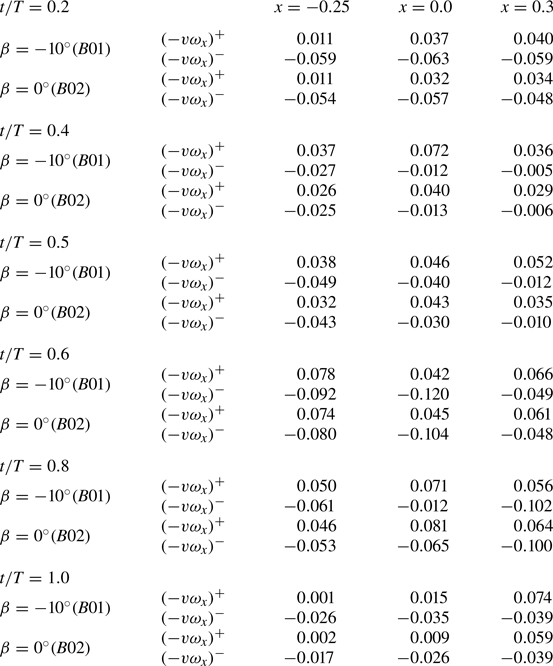
 $-v\omega _x$, especially in figure 15(b). Associating figure 15 with table 9, it can be noted that positive
 $-v\omega _x$ is larger in the slices of the forewing (
 $x=-0.25$), the interface (
 $x=0.0$) and the hindwing (
 $x=0.3$) for the case (
 $B01$) with
 $\beta = -10^{\circ }$ than that for the case
 $B02$ with
 $\beta = 0^{\circ }$. Through the integration of (2.6), we can calculate that the component
 $-v\omega _x$ of the vortex lift coefficients for the forewing and hindwing is 0.030 and 0.054 for the case with
 $\beta = -10^{\circ }$, respectively. The component
 $-v\omega _x$ of the vortex lift coefficients for the forewing and hindwing is −0.002 and 0.038 for the case with
 $\beta = 0^{\circ }$, respectively. It can be seen that the spanwise flow acceleration caused by the slot (dihedral angle
 $\beta = -10^{\circ }$) enhances the vortex lift of both the forewing and hindwing at
 $t/T=0.4$.
Schematic distribution of the component  $-v\omega _x$ in vortex lift for different
 $x$-position slices at
 $t/T = 0.4$: (a–c) dihedral angle
 $\beta = -10^{\circ } (B01)$; (d–f) dihedral angle
 $\beta = 0^{\circ } (B02)$. Case
 $B02$ is the case without a slot.

Surface integral of vortex lift component  $-v\omega _x$ in multiple streamwise slices at
 $t/T=0.4$. The symbol
 $(-v\omega _x)^+$ represents the integral of the positive
 $-v\omega _x$ distributed near the wing, corresponding to the red region in figure 15. The symbol
 $(-v\omega _x)^{-}$ represents the integral of the negative
 $-v\omega _x$ distributed near the wing, corresponding to the blue region in figure 15. The rectangular field of integration of
 $-v\omega _x$ for slices is
 $[-6c,6c]\times [-6c,6c]$ in the spanwise (y) and vertical (z) directions, respectively.

By comparing the dihedral angle  $\beta = -10^{\circ }$ case (figure 16a) with dihedral angle
 $\beta = 0^{\circ }$ case (figure 16d), it can be seen that the streamwise vorticity and the spanwise velocity near the forewing are not affected by the change in the dihedral angle. At the interface between the forewing and hindwing, as shown in figure 16(b,e), we can observe an enhancement in the spanwise velocity
 $v$ for the case with dihedral angle
 $\beta = -10^{\circ }$. From the viewpoint of the vortex dynamics, the strong spanwise velocity contributes to the stabilization of the LEV.
Distribution of the spanwise velocity and streamwise vorticity for different  $x$-position slices at
 $t/T = 0.5$: (a–c) dihedral angle
 $\beta = -10^{\circ } (B01)$; (d–f) dihedral angle
 $\beta = 0^{\circ } (B02)$. Case
 $B02$ is the case without a slot. Contour lines of the spanwise velocity and contours of the streamwise vorticity are shown. The solid and dashed contour lines represent positive and negative spanwise velocity
 $v$, respectively.

In figure 16(c,f), the difference in vortex distribution can be seen near the wingtip. Figure 16(c) reveals the presence of both a vortex  $\text {TV}_{h}$ generated by the hindwing wingtip and a vortex
 $\text {TV}_{f}$ generated by the forewing wingtip above the hindwing, as also observed in the previous analysis of figure 13(a). In figure 16(c), the TV
 $\text {TV}_{f}$ shedding from the forewing is much stronger than that shedding from the forewing in figure 14(c). However, only one TV is present in the hindwing slice for the case without a slot. For the combination term of spanwise velocity and streamwise vorticity
 $-v\omega _x$, the generation of positive vortex lift requires a combination of positive streamwise vorticity and negative spanwise velocity, or of negative streamwise vorticity and positive spanwise velocity. In figure 16(c), the combination of streamwise vorticity and spanwise velocity above the hindwing satisfies the condition for enhancing vortex lift. By contrast, as shown in figure 16(f), only the TV of the hindwing generates vortex lift. Comparing (c) and (f) in figure 17, the positive vortex lift is generated by the TV shedding from the forewing. The additional vortex lift from the shedding TV
 $(-v\omega _x)^+$ at the
 $x = 0.3$ streamwise slice is shown in table 10. The TV detached from the forewing plays a similar function to that of the alula in avian flight found by Lee et al. (Reference Lee, Kim, Park, Jabłoński and Choi2015). Both can enhance lift.
Schematic distribution of the component  $-v\omega _x$ in vortex lift for different
 $x$-position slices at
 $t/T = 0.5$: (a–c) dihedral angle
 $\beta = -10^{\circ } (B01)$; (d–f) dihedral angle
 $\beta = 0^{\circ } (B02)$. Case
 $B02$ is the case without a slot.

Surface integral of vortex lift component  $-v\omega _x$ in multiple streamwise slices at
 $t/T=0.5$. The symbol
 $(-v\omega _x)^+$ represents the integral of the positive
 $-v\omega _x$ distributed near the wing, corresponding to the red region in figure 17. The symbol
 $(-v\omega _x)^{-}$ represents the integral of the negative
 $-v\omega _x$ distributed near the wing, corresponding to the blue region in figure 17. The rectangular field of integration of
 $-v\omega _x$ for slices is
 $[-6c,6c]\times [-6c,6c]$ in the spanwise (y) and vertical (z) directions, respectively.

Similarly, the component  $-v\omega _x$ of the vortex lift coefficient is calculated at
 $t/T=0.5$ on the forewing and hindwing to quantitatively describe the contribution of the shedding TV of the forewing
 $\text {TV}_{f}$ to lift. The component
 $-v\omega _x$ of the vortex lift coefficients for the forewing and hindwing is
 $-$0.012 and 0.083 for the case with
 $\beta = -10^{\circ }$, respectively. The component
 $-v\omega _x$ of the vortex lift coefficients for the forewing and hindwing is
 $-$0.019 and 0.043 for the case with
 $\beta = 0^{\circ }$, respectively. Regardless of the quantitative integral results or the distribution of
 $-v\omega _x$ (figure 17), the slot (dihedral angle) does not significantly affect the component
 $-v\omega _x$ of the vortex lift coefficient for the forewing at
 $t/T=0.5$. For the case with a slot (
 $\beta = -10^{\circ }$), the
 $-v\omega _x$ component of the vortex lift for the total wing is enhanced mainly because the
 $-v\omega _x$ component of the vortex lift for the hindwing is enhanced. Therefore, in the flow field in the case with negative dihedral angle, the shedding TV of the forewing
 $\text {TV}_{f}$ can contribute to the enhancement of vortex lift.
Furthermore, the slot position affects the distribution of the spanwise velocity and streamwise vorticity, which results in the changes to the aerodynamic performance seen in figure 5. As shown in figures 14 and 16, the TVs decreased rapidly after they shed from the forewing. The rapid decreases of the tip vortices indicates that a small-sized hindwing could capture most of the shedding TVs. Considering that the TV capture accounts for a relatively small portion of the time-averaged lift enhancement in the current configurations, the difference between  $x_s =0.4$, 0.2 and
 $0$ is not obvious in figure 5(a). An optimized hindwing size that captures most of the shedding TVs is worth considering in future work.
4. Conclusions
We have investigated the effect of a slot between the forewing and hindwing on the aerodynamic performance of a butterfly-inspired flapping wing model consisting of a flat-plate forewing, hindwing and body. The specific settings of the model have been chosen with reference to previous measurements of butterfly flight. We have used the dihedral angle to quantify the slot between the forewing and hindwing. Aerodynamic forces and vortex structures have been simulated for cases with different parameters related to the slot. By using a lift decomposition formula, the contributions to lift from vortex and inertial forces have been quantified.
The results of this work suggest that the forewing–hindwing interactions of the butterfly-inspired flapping wing differ from those of a dragonfly. Lift can be significantly improved when the slot between the forewing and hindwing is properly configured. The time-averaged lift in the case with the dihedral angle between the forewing and hindwing  $\beta = -10^{\circ }$ is enhanced by approximately 22 % with respect to the case with dihedral angle
 $\beta = 0^{\circ }$, while the time-averaged lift in the case with dihedral angle
 $\beta = 10^{\circ }$ is reduced by approximately 22 % with respect to the case with dihedral angle
 $\beta = 0^{\circ }$.
The vortex dynamic mechanisms underlying lift enhancement have been identified for the butterfly-inspired flapping wing. The hindwing, being lower than the forewing, generates a streamwise ram effect for the flow beneath the forewing. This streamwise ram effect decreases the streamwise velocity beneath the forewing, resulting in an enhancement of vortex lift. Meanwhile, wake capture involving the TV is found for the butterfly-inspired flapping wing, differing from the wake capture of a dragonfly. When the hindwing is lower than the forewing, the TV shedding from the forewing contributes to the enhancement of vortex lift in the combination of the spanwise velocity and streamwise vorticity above the hindwing.
To the best of our knowledge, this study is the first to pay attention to the effects of a slot between the forewing and hindwing inspired by butterfly flight, and it has revealed how the slot has a remarkable effect on the aerodynamic performance of a butterfly-inspired flapping wing.
The present work does, however, have some limitations and shortcomings. The butterfly-inspired flapping wing model studied in this paper is always in a uniform incoming flow environment, as a consequence of which the thrust effect of the upstroke is not realized. The gap of the slot studied here is fixed throughout the wingbeat, which might be different from actual butterfly flight. The current butterfly-inspired flapping wing model is constructed based on a simplified model proposed by previous work with a wing shape that differs from that of a real butterfly, although the aspect ratio and the basic motion parameters are realistic.
In the future, we will improve the model to incorporate a more realistic wing shape, as well as adopting an autonomous propulsion mode to test the effect of the wing slot on climbing performance. It also needs to be investigated whether the lift enhancement resulting from the presence of the slot can be achieved in the case of a larger-aspect-ratio wing.
Acknowledgements
We thank Z. Zhou for the butterfly illustration.
Funding
This work is supported by the NSFC Basic Science Center Program for ‘Multiscale Problems in Nonlinear Mechanics’ (grant no. 11988102); the National Natural Science Foundation of China (grant nos 92252203, 12102439 and 12425207); the Chinese Academy of Sciences Project for Young Scientists in Basic Research (grant no. YSBR-087); and the Strategic Priority Research Program of Chinese Academy of Sciences (grant no. XDB0620102).
Declaration of interests
The authors report no conflict of interest.
Data availability statement
The data that support the findings of this study are available from the corresponding authors upon reasonable request.
Appendix A. Examination of the lift decomposition formula
In this appendix, we report the comparison between the lift calculated by the integration of body force and that obtained from lift decomposition formula (2.5). We report the comparison of the case  $B02$ (the case with
 $\beta =0^{\circ }$) as an example. As shown in figure 18(a), the reference curve represents the integral of the body force applied near the boundary in the vertical (
 $z$) direction as calculated by the immersed boundary method. The square scatter is calculated from the lift decomposition (2.5) based on the velocity and vorticity. In figure 18(a), the lift force obtained from the integration of the body force is in good agreement with that obtained from the lift decomposition formula. The maximum difference in the lift coefficient calculated in (2.5) and the lift coefficient obtained by body force integration is within
 $0.005$, i.e. approximately
 $1\,\%$ of the peak lift coefficient obtained by body force integration. It confirms the validity of the lift decomposition formula under the present conditions. Here, a rectangular volume is employed in decomposing the lift. The upper boundary of the control volume in the streamwise direction is adjusted to the maximum streamwise position of the trailing edge, to avoid the effect of wake on the integration result. When the lift decomposition formula is applied to the lift calculation of case
 $B02$ (the case with
 $\beta =0^{\circ }$), the control volume is set to
 $[-4c,(1+\sqrt {3})c/4]\times [-6c,6c]\times [-6c,6c]$ in the streamwise (
 $x$), spanwise (
 $\kern 1.5pt y$) and vertical (
 $z$) directions for three-dimensional flows.
(a) Schematic diagram of lift force based on the velocity and vorticity (lift decomposition formula) and lift force from the integration of body force (reference). (b) The result of the lift decomposition formula calculated by (2.5).

In figure 18(b), based on the velocity and vorticity of case  $B02$ (the case with
 $\beta =0^{\circ }$), the contributions of the terms of (2.5) are presented to examine the validity of (2.6). According to the right-hand terms of (2.5), we know that the lift force acting on the butterfly-inspired flapping wing consists of five components. The five components are
 $A:\rho \int _{V_{f}}\boldsymbol {u}\times \boldsymbol {\omega }\,\mathrm {d}V$,
 $B: - \rho \int _{V_{f}}{\partial {\boldsymbol {u}}}/{\partial {t}}\,\mathrm {d}V$,
 $C: -\oint _{\varSigma }(p+{\rho q^2}/{2})\boldsymbol {n}\,\mathrm {d}S$,
 $D: \oint _{\varSigma }\boldsymbol {\tau } \,\mathrm {d}S$,
 $E: - {\rho } \oint _{\partial {B}}({q^2}/2)\boldsymbol {n}\,\mathrm {d}S$. As shown in figure 18(b), the sum of the terms
 $C$ ,
 $D$ and
 $E$ accounts for an almost negligible proportion of the integral result of the lift decomposition formula. In (2.5), the
 $A:\rho \int _{V_{f}}\boldsymbol {u}\times \boldsymbol {\omega }\,\mathrm {d}V$ vortex lift term and
 $B: - \rho \int _{V_{f}}{\partial {\boldsymbol {u}}}/{\partial {t}}\,\mathrm {d}V$ inertial force term dominate the integration result for lift decomposition. The maximum difference in lift obtained by (2.5) and (2.6) is within 0.015, i.e. 4
 $\,\%$ of the peak lift coefficient obtained by (2.5). Therefore, for the control volume in the present work, the sum of the lift components in (2.6) can be considered to be equal to the lift force acting on the flapping wing.
Appendix B. Convergence study of spatial resolution and temporal resolution
We report the convergence study of spatial resolution and temporal resolution in this appendix. The mesh convergence study is performed with four spatial resolutions, namely,  $h = 0.05c$,
 $h = 0.025c$,
 $h = 0.0125c$ and
 $h = 0.01c$. Here,
 $h$ denotes the minimum mesh size of the Eulerian mesh. Two typical cases (cases
 $B01$ (
 $\beta =-10^{\circ }$) and
 $B02$ (
 $\beta =0^{\circ }$)) are simulated on the four spatial resolutions, respectively. The lift coefficient and drag coefficient curves are shown in figure 19(a,b), respectively. In figure 19, the lift and drag coefficients obtained by the present numerical simulations with three spatial resolutions are compared. The effect of spatial resolution on lift and drag is quantitatively analysed using case
 $B01$ as an example. The time-averaged lift and drag for case
 $B01$ at spatial resolution
 $h = 0.05c$ differ by 7.0 % and 9.2 %, respectively, compared with the time-averaged lift and drag for
 $h = 0.025c$. The time-averaged lift and drag for case
 $B01$ at spatial resolution
 $h = 0.0125c$ differ by 2.5 % and 1.3 %, respectively, compared with the time-averaged lift and drag for
 $h = 0.025c$. The mesh convergence study shows that the solutions are converged when
 $h = 0.025c$, which agrees with
 $h = 0.0125c$.
Cases  $B01$ (
 $\beta =-10^{\circ }$) and
 $B02$ (
 $\beta =0^{\circ }$) are simulated for the three spatial resolution settings. Here,
 $h$ denotes the minimum mesh size of the Eulerian mesh. The time history of (a) the lift coefficient and (b) the drag coefficient.

In order to examine the spatial resolution of the mesh at the wing slot, the Eulerian mesh with  $h = 0.01c$ is also used. In figure 20, the lift and drag coefficients obtained by the present numerical simulations with three spatial resolutions are compared. The effect of spatial resolution on lift and drag is quantitatively analysed using case
 $B01$ as an example. The time-averaged lift and drag for case
 $B01$ at spatial resolution
 $h = 0.01c$ differ by 2.3 % and 1.6 %, respectively, compared with the time-averaged lift and drag for
 $h = 0.025c$. The results for the three Eulerian mesh sizes (
 $h = 0.01c$,
 $h=0.0125c$,
 $h=0.025c$) indicate that the difference between the total aerodynamic forces is ignorable. We would like to point out that these mesh sizes might not be fine enough to resolve the details of the shear layers near the slot, which is currently outside of the scope of the present work.
Cases  $B01$ (
 $\beta =-10^{\circ }$) and
 $B02$ (
 $\beta =0^{\circ }$) are simulated for the three spatial resolution settings. Here,
 $h$ denotes the minimum mesh size of the Eulerian mesh. The time history of (a) the lift coefficient and (b) the drag coefficient.

The independence of the results from temporal resolution is also examined for the present flapping wing model. The convergence study of the temporal resolution is carried out based on the Eulerian mesh with a minimum mesh size  $h = 0.025c$. Three difference temporal resolutions are set,
 $dt=0.014$,
 $dt=0.010$ and
 $dt=0.007$. The temporal resolution is set in accordance with recommended guidelines of the International Towing Tank Conference (ITTC 2021). The lift and drag coefficients for the three temporal resolutions are shown in figures 21 and 22.
(a) Lift coefficient curves within ten flapping periods for case  $B01$ (dihedral angle
 $\beta =-10^{\circ }$) at three temporal resolution settings. (b) Drag coefficient curves within ten flapping periods for case
 $B01$ (dihedral angle
 $\beta =-10^{\circ }$) at three temporal resolution settings.

(a) Lift coefficient curves during the fourth flapping period for case  $B01$ (dihedral angle
 $\beta =-10^{\circ }$) at three temporal resolution settings. (b) Drag coefficient curves during the fourth flapping period for case
 $B01$ (dihedral angle
 $\beta =-10^{\circ }$) at three temporal resolution settings.

The results in figures 21 and 22 show that the current temporal resolution has converged the calculations. The time-averaged lift coefficients at temporal resolutions  $dt = 0.014$ and
 $dt = 0.007$ differ by less than 0.2 % compared with the time-averaged lift coefficient at temporal resolution
 $dt = 0.01$. The lift coefficients for three temporal resolution settings are almost identical. The time-averaged drag coefficients at temporal resolutions
 $dt = 0.014$ differ by less than 2.0 % compared with the time-averaged drag coefficient at temporal resolution
 $dt = 0.01$. The time-averaged drag coefficients at temporal resolutions
 $dt = 0.007$ differ by less than 0.8 % compared with the time-averaged drag coefficient at temporal resolution
 $dt = 0.01$. Therefore, the temporal resolution
 $dt = 0.010$ is applied in the present study.
Appendix C. Lift of the cases with a slot at other mean elevation angles of the forewing  $\varPsi _{f0}$

We perform the validation that the wing slot can still significantly affect the lift at other mean elevation angles of the forewing  $\varPsi _{f0}$ in this appendix. All three cases in figure 23(a) have the same mean elevation angle of the forewing
 $\varPsi _{f0}=10^{\circ }$, and controlling the mean elevation angle of the hindwing changes the dihedral angles
 $\beta$ between the forewing and hindwing. Consistent with the phenomenon in the main text, a dihedral angle
 $\beta =-10^{\circ }$ will result in greater lift than the case
 $B26$ without a slot. A dihedral angle
 $\beta =10^{\circ }$ will result in lower lift than the case
 $B26$ without a slot. The time-averaged lift coefficients for cases
 $B34$ and
 $B35$ are 0.282 and 0.171, respectively.
(a) Lift coefficients of butterfly-inspired flapping wing with  $\varPsi _{f0}=10^{\circ }$. Case
 $B26$ (
 $\beta =0^{\circ }$) is the case without a slot. (b) Lift coefficients of butterfly-inspired flapping wing with
 $\varPsi _{f0}=-10^{\circ }$. Case
 $B27$ (
 $\beta =0^{\circ }$) is the case without a slot.

Similarly, in figure 23(b), all the cases have the same mean elevation angle of the forewing  $\varPsi _{f0}=-10^{\circ }$. A dihedral angle
 $\beta =-10^{\circ }$ still results in more lift than the case
 $B27$ without a slot. The time-averaged lift coefficients for cases
 $B36$ and
 $B37$ are 0.278 and 0.180, respectively.
Appendix D. The difference in aerodynamic forces between the butterfly-inspired flapping wing model and square flapping wing
We report the aerodynamic difference between our butterfly-inspired flapping wing model and a square flapping wing in this appendix. In figure 24(a), it can be seen from the tiled diagram that the trailing edge of the forewing does not coincide with the leading edge of the hindwing for our butterfly-inspired flapping wing model. In the case of a square flapping wing (figure 24b), the overlap between the trailing edge of the forewing and the leading edge of the hindwing will result in an inconvenient setting of the dihedral angle  $\beta$.
(a) Tiled diagram of the butterfly-inspired flapping wing model. The angle between the trailing edge of the forewing and the leading edge of the hind wing is  $5.7^{\circ }$. (b) Tiled diagram of a square flapping wing.

Lift and drag coefficients are shown in figure 25 for the butterfly-inspired flapping wing model and square flapping wing. For these two cases, the lift coefficients are generally consistent. The time-averaged lift coefficients for case  $B02$ and the square flapping wing are 0.236 and 0.238, respectively. The time-averaged drag coefficients for case
 $B02$ and the square flapping wing are 0.190 and 0.205, respectively. The drag coefficient for the square flapping wing increases by 8 % compared with case
 $B02$.
(a) Lift coefficients of butterfly-inspired flapping wing (case  $B02$) and square flapping wing. Case
 $B02$ (
 $\beta =0^{\circ }$) is the case without a slot. (b) Drag coefficients of butterfly-inspired flapping wing (case
 $B02$) and square flapping wing.

Appendix E. The integral of the vortex lift components for multiple wing sections over the flapping cycle and the spanwise vorticity distribution used for circulation integration
We present surface integrals of the components  $u\omega _y$ and
 $-v\omega _x$ of the vortex lift at multiple wing sections for multiple instants in this appendix. In table 11,
 $u\omega _y$ is split into
 $(u\omega _y)^+$ and
 $(u\omega _y)^{-}$, i.e.
 $u\omega _y=(u\omega _y)^++(u\omega _y)^{-}$. Here,
 $(u\omega _y)^+$ represents the surface integral result for positive
 $u\omega _y$ (the red area in
 $u\omega _y$ contours) within a slice and
 $(u\omega _y)^{-}$ represents the surface integral result for negative
 $u\omega _y$ (the blue area in
 $u\omega _y$ contours) within a slice.
Surface integral of vortex lift component  $u\omega _y$ in multiple spanwise slices at multiple instants.

Similarly, we perform surface integrals of  $-v\omega _x$ within the streamwise slices (
 $x=-0.25$,
 $x=0.0$ and
 $x=0.3$) for multiple instants in table 12. Here,
 $(-v\omega _x)^+$ represents the surface integral result for positive
 $-v\omega _x$ (the red area in
 $-v\omega _x$ contours) within a slice and
 $(-v\omega _x)^{-}$ represents the surface integral result for negative
 $-v\omega _x$ (the blue area in
 $-v\omega _x$ contours) within a slice.
Surface integral of vortex lift component  $-v\omega _x$ in multiple streamwise slices at multiple instants.

In addition, we also present here the spanwise vorticity distributions used for calculating the circulations of the LEV in tables 5 and 6. The spanwise slices at 75 % wingspan for eight instants are shown in figures 26 and 27. Above the forewing, the LEVs within the  $Q = 6$ isoline are integrated, corresponding to the circulations of the LEV presented in tables 5 and 6.
Contours of spanwise vorticity  $\omega _y$ for 75 % wingspan slice at
 $t/T=$ 0.1, 0.2, 0.3 and 0.4. The white isoline denotes
 $Q=6$. (a) Case
 $B01$ with dihedral angle
 $\beta = -10^{\circ }$; (b) case
 $B02$ with dihedral angle
 $\beta = 0^{\circ }$.

Contours of spanwise vorticity  $\omega _y$ for 75 % wingspan slice at
 $t/T= 0.6$, 0.7, 0.8 and 0.9. The white isoline denotes
 $Q=6$. (a) Case
 $B01$ with dihedral angle
 $\beta = -10^{\circ }$; (b) case
 $B02$ with dihedral angle
 $\beta = 0^{\circ }$.