


I. INTRODUCTION
Interest of silicon–germanium (SiGe) heterostructures on silicon for optical receivers in short-wavelength (850 nm) transmission systems and networks is well recognized [Reference Pei1]. Its main advantages are improved speed and responsivity combined with cost effectiveness and the ability to be integrated in high-speed silicon analog or digital circuits. Several structures were proposed [Reference Pei2, Reference Lai, Huang and Hsu3].
We have designed and characterized a new structure of SiGe heterojunction bipolar phototransistor (HPT), showing a significant dependence of its internal characteristics (mainly the collector-to-base capacitance and the time constants of the current source), with the received light power, which was not reported until now. It can be used in the new receiver structure for optics–microwave interfacing in radio-over-fiber networks we have previously proposed [Reference Egels, Delacressonnière, Sahabun and Lecoy4]. It is based on a photo-oscillator designed to operate at a central frequency that can be chosen in the range of 5–12 GHz. A frequency deviation of several tens of MHz may be controlled by illumination. In this paper, we investigate thoroughly the HPT by itself, mainly its equivalent circuit variations under illumination, to derive what might be the maximum frequency deviation of a photo-oscillator in which the HPT would be the key component, but could have many other applications [Reference Polleux, Paszkiewicz, Billabert, Salset and Rumelhard5].
The phototransistor was designed by modifying a heterojunction bipolar transistor (HBT) in 0.35 µm commercially available technology from AMS (Austria Mikro Systems). Removing a base finger creates an illumination window. This structure was improved since the first one [Reference Lecoy and Delacressonnière6], in order to enhance the efficiency without degrading the transition frequency: the main modification consists of an increase in the transistor length to get a larger illuminated area. Nevertheless, we chose not to increase the dimension of the illumination window in the other direction to preserve the transition frequency of the device and to remain compatible with commercial RF Foundry services, in contrast with other designs aiming to optimize the responsitivity [Reference Schiellein7]. Its geometry makes it also suitable as an integrated receiver in optical network-on-chip (ONoC) on silicon using optical planar waveguides.
New measurements reported here concern the HPT equivalent elements depending on the photocurrent induced by the received light and on the bias point. These measurements have confirmed the possibility to use it as active element of a photo-oscillator whose oscillation frequency decreases linearly with the received power, converting an OOK optical signal into a frequency or phase-modulated radio frequency (RF) carrier. This detection scheme could be an interesting and cost-effective alternative to RF transmission over fiber [Reference Jenmisson8].
II. The HPT
Its base has a gradual Ge concentration up to Si0.8Ge0.2, and a thickness of about 10 nm. Its sensitivity is high up to a wavelength of 0.95 µm [Reference Polleux and Rumelhard9], which is suitable for low cost, high bit-rate large area networks (LANs) using Vertical Cavity Surface-Emitting Laser (VCSEL) transmitters at 0.85 µm. To transform the HBT into an HPT with improved detection efficiency, the metallization of one base finger was suppressed and the length of the illuminated zone was increased up to 12 µm (Fig. 1).
Layout of the phototransistor.

We have experimentally verified that the intrinsic characteristics of the transistor were not modified. Alone among extrinsic elements, the base access resistance R b1 increases significantly (from 25 to 60 Ω), due to the suppression of a metallization finger.
III. STATIC MEASUREMENTS
The phototransistor was characterized on a test bench and was illuminated through a tapered multimode fiber powered by a 0.85 µm VCSEL at its other end. Static measurement of the photocurrent I PH was performed in photodiode mode (V be = 0) depending on the optical power P at the fiber end (Fig. 2). The characteristic is rather linear with a slight saturation effect at high illumination. The measured responsivity is R = 0.066 A/W, thus an external efficiency of 15% with respect to its theoretical value [Reference Lecoy and Delacressonnière6], this low value is simply due to the non-optimization of the fiber-to-detector coupling. In a previous experiment, we had achieved a higher efficiency (R = 0.15 A/W) with a sharper fiber end. Due to the internal structure of the phototransistor (directly derived from a foundry transistor) and its optimization in transition frequency, no gain was observed in the phototransistor mode compared to the photodiode mode, as in [Reference Polleux, Paszkiewicz, Billabert, Salset and Rumelhard5, Reference Polleux10, Reference Moutier, Polleux, Rumelhard and Schumacher11]. But our purpose was to use the phototransistor as a tunable oscillator, not as amplifier.
Photocurrent I PH versus received power P.

Another set of measurements concerned the emitter-to-base static characteristics (Fig. 3). It shows in the dark the classical nkT log shape of a diode with n ≈ 2.8 (instead of 2 in [Reference Pei2]), but when illuminated with 950 µW, a current rather proportional to V be is superposed to the diode current, at least below base-emitter diode threshold voltage, which can be modeled by a photo conductance in parallel with the diode.
Base to emitter junction characteristics.

IV. EQUIVALENT PARAMETERS MEASUREMENTS
A) Modelling
We used the classical model shown in Fig. 4 and the methods developed for its parameters extraction [Reference Basaran, Wieser, Feiler and Berroth12–Reference Rudolph, Doerner and Heymann15]. Measurements of the Z-matrix (extracted from the S-matrix over the 1.5–20 GHz range, after an Line, Reflect, Match (LRM) calibration of the HP8510C VNA) allow the determination of following elements:
R b1 is the physical access resistance, it is near 60 Ω and rather less dependent on bias and received optical power P;
R b2 and R e correspond to the base-to-emitter junction, they follow the classical nkT/qI b law; moreover, the emitter resistance R e decreases when P increases, which is due to photoconductivity;
C e has a negligible admittance (Z e is quasi-real) and cannot be significantly extracted from measurement with accurate values;
Equivalent model of the phototransistor.

R c is quasi-infinite (Z c is quasi-imaginary and represented by C c) and cannot be extracted from measurement with accurate values either; it should be kept in mind that element values extracted from S-parameters cannot be determined accurately when their impedance is either very high or very low with respect to the reference impedance, which is the present case; and the current gain α and time constants τ1 (delay) and τ2 (relaxation time) come from:

with α0 ≈ 0.995 corresponding to static β ≈ 200.
B) Results
Measurements of these parameters were performed in the range 1.5–20 GHz at different biasing points versus optical power P. The most significant results concern the capacitance C c (Fig. 5) and delay time τ1 (Fig. 6), which both increase significantly and rather linearly with the received power P. We have also extracted the parallel capacitance C b′e of a classical Giacoletto scheme [Reference Giacoletto16], which was also found to be increasing rather linearly with P (Fig. 7), enabling the decreasing of the photo-oscillator frequency under illumination.
Variation of capacitance C c with the received power P.

Variation of time constant τ1 with the received power P.

Variation of parallel capacitance C b′e with received power P.
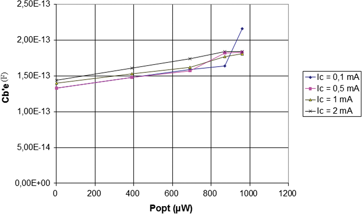
The physical reason for all these effects could be the decrease in the depletion width under optical injection. τ1 decreases when I c increases (τ2, which is an Resistance-Capacitor (RC) time constant, remains nearly constant). It allows the design of a photo-oscillator whose frequency decreases when the optical power increases, which was demonstrated by simulation [Reference Egels, Delacressonnière, Sahabun and Lecoy4]. C c decreases when the bias voltage V ce increases.
C) Transition frequency
Derived from the S-matrix, transition frequency was found to be in the range of 20–50 GHz depending on the biasing point, increasing strongly with I c (it reaches 50 GHz at I c = 2 mA). It decreases slightly when P increases, which is correlated to the capacitance increase.
V. CONCLUSION
The experiments performed on the prototypes of this new phototransistor confirm its ability to be the active element of a light-controlled photo-oscillator for optical–microwave interfacing in hybrid access networks, as well as other devices such as integrated photo-receivers for ONoC.
ACKNOWLEDGEMENTS
We thank the graduate students from ENSEA and partner universities (Barcelona, Spain and Iaşi, Romania) who participated in the design and measurements. We also thank J.-L. Polleux, A.L. Billabert and C. Rumelhard (Esycom, France) for fruitful discussions.
 Pierre Lecoy was born in 1955 in Argenteuil (France) and graduated from Ecole Centrale Paris (ECP), 1976 and PhD in electronics from University Paris VI (1980). He was researcher at France-Telecom R&D and at Alcatel and since 1984 is Professor at Ecole Centrale de Paris and member of the research lab ETIS at Cergy-Pontoise. His research fields include fiberoptic sensors and then optics–microwave interfacing. Professor Lecoy is member of EOS and author of “Fiberoptic communications”, Wiley, 2008.
 Bruno Delacressonniere was born in 1962 in Valenciennes (France) and graduated from Institut Supérieur d'Electronique du Nord (ISEN), 1985 and PhD in physics from University Lille I (1988). He was Associate Professor at ESEO (Angers, France) between 1988 and 1990 and then at ENSEA (Cergy, France), and member of the research lab LaMIPS, Caen, France. His research fields include optics–microwave interfacing and monolithic active filtering.
 Daniel Pasquet was born in 1948 in Aulnay-sous-Bois, France and gained his French diplôme d'ingénieur in 1970 at ENREA, Clichy, France and his PhD at Lille 1 University in 1975. He had been an assistant professor at IUT Calais France from 1971 to 1981. He joined ENSEA, Cergy, France in 1981, where he has been a professor since 1987. He headed ENSEA microwave lab from 1983 to 1992 and from 2002 to 2005. He had been ENSEA vice-director in charge of research from 1998 to 2007. He is currently a researcher at LaMIPS, Caen, France. Daniel Pasquet's research fields are microwave measurements and passive components modeling. He is author or co-author of 180 papers and communications. Daniel Pasquet was IEEE France Section chair and is currently Microwave Theory and Technique Society (MTT-S) Region 8 chapter coordinator. He is member of the MTT-11 measurements technical committee.



