



1. Introduction
In the last decade neural networks have been successfully exploited to solve a variety of practical problems, ranging from computer vision and speech recognition to feature extraction [Reference Goodfellow, Pouget-Abadie, Mirza, Xu, Warde-Farley, Ozair, Courville and Bengio14, Reference LeCun, Bengio and Hinton19]. This has stimulated new mathematical research in different fields such as probability and statistics, with the final goal of better understanding how neural networks work and how to make them more efficient [Reference Apollonio, De Canditiis, Franzina, Stolfi and Torrisi1, Reference Balasubramanian, Goldstein, Ross and Salim2, Reference Braun, Kohler, Langer and Walk6, Reference Basteri and Trevisan3, Reference Bordino, Favaro and Fortini5, Reference Cammarota, Marinucci, Salvi and Vigogna7, Reference Eldan, Mikulincer and Schramm10, Reference Favaro, Fortini and Peluchetti11, Reference Favaro, Hanin, Marinucci, Nourdin and Peccati12, Reference Hanin15, Reference Hirsch and Willhalm17, Reference Jung, Lee, Lee and Yang18, Reference Sirignano and Spiliopoulos24, Reference Vogel25, Reference Zavatone-Veth and Pehlevan26]. Indeed, despite their profound engineering success, a comprehensive understanding of the intrinsic working mechanism of neural networks is still lacking. In particular, the analysis of deep neural networks is very challenging due to the recursive and nonlinear structure of the models.
Neural networks are parametrized families of functions that are typically used in statistical learning to estimate an unknown function f. In practice, we first fix the network architecture, specifying the family of parametric functions, and then look for an approximation of the target function f, within the specified family, on the basis of a given set of training data [Reference Roberts, Yaida and Hanin22].
In this paper, we focus on the class of fully connected neural networks, which are formally defined as follows. Fix a positive integer
 $L\geq 1$
,
 $L+2$
positive integers
 $n_0, n_1,\ldots,n_{L+1}$
, and a function
 $\sigma\colon\mathbb R\to\mathbb R$
. A fully connected neural network with depth L, input dimension
 $n_0$
, output dimension
 $n_{L+1}$
, hidden layer widths
 $n_1,\ldots,n_L$
, and pre-activation function
 $\sigma\colon\mathbb R\to\mathbb R$
is a function
 $$x=(x_{1},\ldots,x_{n_0})\in T\subset\mathbb{R}^{n_0}\mapsto Z^{(L+1)}(x) =\big(Z_1^{(L+1)}(x),\ldots,Z_{n_{L+1}}^{(L+1)}(x)\big)\in\mathbb{R}^{n_{L+1}}$$
defined by
 \begin{equation} \begin{cases} Z_i^{(1)}(x) = b_i^{(1)} + \sum_{r=1}^{n_0}W_{ir}^{(1)}x_r, & i=1,\ldots,n_1, \\[3pt] Z_i^{(\ell+1)}(x) = b_i^{(\ell+1)} + \sum_{j=1}^{n_\ell}W_{ij}^{(\ell+1)}\sigma\big(Z_j^{(\ell)}(x)\big), & i=1,\ldots,n_{\ell+1},\ 1\leq\ell\leq L, \end{cases}\end{equation}
where
 $\big\{b_i^{(\ell)}\big\}$
(network biases) and
 $\big\{W_{ij}^{(\ell)}\big\}$
(network weights) are the network parameters. Then, for fixed L and
 $n_1,\ldots, n_L$
(i.e. for a fixed network architecture) and given a training dataset
 $\{(x_\alpha,f(x_\alpha))\}_{\alpha=1,\ldots,m}$
,
 $m\geq 1$
, we look for biases and weights such that
 $Z^{(L+1)}(x_\alpha)\, \approx \, f(x_\alpha)$
for inputs
 $x_\alpha$
not only within but also outside the training dataset. To this end, the usual procedure consists of two steps: (i) randomly initialize the network parameters
 $\big\{b_i^{(\ell)}\big\}$
and
 $\big\{W_{ij}^{(\ell)}\big\}$
; (ii) optimize the parameters by minimizing some empirical risk function (such as the squared error).
Therefore, to understand the behavior of a fully connected neural network at the start of training, we study fully connected neural networks with random biases and random weights. In most papers in the literature, the network parameters are assumed to be Gaussian distributed (see, e.g., [Reference Apollonio, De Canditiis, Franzina, Stolfi and Torrisi1, Reference Balasubramanian, Goldstein, Ross and Salim2, Reference Basteri and Trevisan3, Reference Bordino, Favaro and Fortini5, Reference Favaro, Hanin, Marinucci, Nourdin and Peccati12, Reference Hanin15, Reference Roberts, Yaida and Hanin22]); more specifically, for
 $C_b\geq 0$
and
 $C_W>0$
, it is supposed that:
-
• the random variables
 $b_i^{(\ell)}$
are centered normal distributed with variance
$C_b$
(
$1\leq \ell\leq L$
);
-
• the random variables
$W_{ij}^{(\ell+1)}$
are centered normal distributed with variance
$C_W/n_\ell$
(
$0\leq\ell\leq L$
); -
• all these random variables are independent.


If
 $L\geq 2$
these neural networks are called Gaussian fully connected deep neural networks; if
 $L=1$
they are called Gaussian fully connected shallow neural networks.
In the literature there is a considerable number of papers that investigate the asymptotic behavior of fully connected neural networks. Most of them focus on the distribution approximation of the output in the infinite width limit, i.e. when the parameters
 $n_1,\ldots,n_L$
tend to infinity. In the context of shallow neural networks, a seminal paper in this direction is [Reference Neal and Neal21]; see [Reference Balasubramanian, Goldstein, Ross and Salim2, Reference Cammarota, Marinucci, Salvi and Vigogna7, Reference Eldan, Mikulincer and Schramm10] for related contributions. An important recent result is [Reference Hanin15, Theorem 1.2], which provides, when T is compact, the weak convergence of
 $\big(\big(Z_h^{(L+1)}(x)\big)_{x\in T}\big)_{h=1,\ldots,n_{L+1}}$
to a suitable centered Gaussian field (on T), as
 $n_1,\ldots,n_L\to\infty$
, for every arbitrarily fixed
 $L\geq 1$
and for continuous and polynomially bounded pre-activation functions. Quantitative versions of this result, with respect to different probability metrics, are given in [Reference Apollonio, De Canditiis, Franzina, Stolfi and Torrisi1, Reference Basteri and Trevisan3, Reference Bordino, Favaro and Fortini5, Reference Favaro, Hanin, Marinucci, Nourdin and Peccati12]. We emphasize that in [Reference Favaro, Hanin, Marinucci, Nourdin and Peccati12] the authors study the Gaussian approximation of the sensitivities of the output with respect to the input, i.e. the Gaussian approximation of the mixed directional derivatives of the output with respect to the input. Large-width asymptotics of fully connected deep neural networks with biases and weights distributed according to a non-Gaussian stable law are investigated in [Reference Favaro, Fortini and Peluchetti11, Reference Jung, Lee, Lee and Yang18]. The output distribution of a Gaussian fully connected deep neural network, with finite hidden layer widths and a ReLU pre-activation, has been studied in [Reference Zavatone-Veth and Pehlevan26].
In this paper we are interested in a different kind of asymptotic result, based on the theory of large deviations [Reference Dembo and Zeitouni9]. Such a theory allows us to quantify the atypical behavior of the network, and provides probability estimates of rare events on an exponential scale. Among the references on large deviations on this topic we recall [Reference Li and Saad20] (which concerns a deep neural network model different from (1)) and [Reference Hirsch and Willhalm17] (whose context is different from ours, indeed it concerns the stochastic gradient descent for trained shallow neural networks with quadratic loss).
In this paper we set
 $n_\ell=n_\ell(n)$
 $(\ell=1,\ldots,L)$
, assume that the sequences
 $n_\ell$
diverge to infinity (as
 $n\to\infty$
), and, for a suitable normalizing sequence
 $v_n^*\to\infty$
(see Condition 2), a finite set A, and
 $T\equiv\{x_\alpha\}_{\alpha\in A}$
(therefore T is also finite), we provide the following main results for suitable sequences of
 $\mathbb{R}^{|A|\times n_{L+1}}$
-valued random variables (and we shall often use the indices
 $\alpha h$
to mean
 $(\alpha,h)\in A\times\{1,\ldots,n_{L+1}\}$
):
-
• The large-deviation principle of the sequence
(2)with speed
\begin{equation} \big\{\big(Z_h^{(L+1)}(x_\alpha)/\sqrt{v_n^*}\big)_{\alpha h}\big\}_n \end{equation}
$v_n^*$
(see Theorem 1).
-
• For every sequence of positive numbers
$\{a_n\}_n$
such that (3)the large-deviation principle of the sequence
\begin{equation} a_n\to 0\quad\mbox{and}\quad a_nv_n^*\to\infty\quad\text{as $n\to\infty$},\end{equation}
(4)with speed
\begin{equation}\big\{\big(\sqrt{a_n}Z_h^{(L+1)}(x_\alpha)\big)_{\alpha h}\big\}_n\end{equation}
$1/a_n$
(see Theorem 2).


We remark that the sequences in (2) and (4) converge to the null matrix
 $0\in\mathbb{R}^{|A|\times n_{L+1}}$
, where
 $|A|$
denotes the cardinality of A. The class of large-deviation principles in the second result is known in the literature as a moderate-deviation principle and fills the gap between the convergence in probability to
 $0\in\mathbb{R}^{|A|\times n_{L+1}}$
of the sequence in (2) and the convergence in law of the sequence
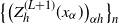 $\big\{\big(Z_h^{(L+1)}(x_\alpha)\big)_{\alpha h}\big\}_n$
to a Gaussian vector. We remark that moderate-deviation estimates (and concentration inequalities) for the output of a Gaussian neural network might be proved even applying the classical theory on the subject developed in [Reference Saulis and Statulevičius23]. To apply this theory, we need a fine study of the cumulants of the output. To this end, the main findings in [Reference Hanin16] seem not to be useful as they do not provide the constants involved in the big-O functions that give the rate of the cumulants. This could be a topic for future research.
The proofs of our main results proceed by induction on the number of layers and combine a representation of Gaussian fully connected deep neural networks (see Lemma 3) with a large-deviation principle on product spaces proved in [Reference Chaganty8] (see Proposition 1). These results hold when the pre-activation function is bounded and continuous, and therefore exclude some important classes of pre-activations such as the ReLU function. However, we are able to provide large- and moderate-deviation principles for Gaussian fully connected deep neural networks with a single input and a ReLU pre-activation (see Section 4). Indeed, if
 $|A|=1$
, some technical difficulties encountered in the general case can be overcome by means of ad hoc arguments. Recently, our result for the case of a ReLU function has been generalized in [Reference Vogel25], which considers Gaussian fully connected deep neural networks with linearly growing pre-activation functions.
For the case of Gaussian shallow neural networks, i.e. if
 $L=1$
, the model is much simpler. In such a case we are able to prove large and moderate deviations for the output and its sensitivity (i.e. the derivative of the output with respect to the input) under quite general assumptions on
 $\sigma$
(see Propositions 2, 3, and 4).
The paper is structured as follows. In Section 2 we give the statements of the main results, together with the preliminary notation and some remarks. The proofs of the main results are presented in Section 3. The particular case of a Gaussian fully connected deep neural network with a single input and ReLU pre-activation function is treated in Section 4. Finally, large and moderate deviations for Gaussian shallow neural networks and their sensitivities are presented in Section 5.
2. Main results: Statements and remarks
We start with some preliminary notation and the hypotheses. In our main results we assume that Condition 1 holds.
Condition 1. The function
 $\sigma$
is continuous and bounded. In particular, we set
 $\|\sigma\|_\infty \, :\! = \,\sup_{x\in\mathbb{R}}|\sigma(x)|$
.
As mentioned in the introduction, we take
 $T \, :\! = \,\{x_\alpha\}_{\alpha\in A}$
with
 $x_\alpha=(x_{\alpha,1},\ldots,x_{\alpha,n_0})\in\mathbb{R}^{n_0}$
for some finite set A. Moreover, we use the simplified notation
 $\underline{x}$
to mean
 $T=\{x_\alpha\}_{\alpha\in A}$
.
It is well known (see, e.g., [Reference Bathia4, Section I.2]) that, for every symmetric positive semidefinite matrix
 $q=(q_{\alpha\beta})_{\alpha,\beta\in A}$
, there exists a unique symmetric positive semidefinite matrix
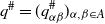 $q^\#=(q_{\alpha\beta}^\#)_{\alpha,\beta\in A}$
such that
 $q^\# q^\#=q$
, i.e.
 $q_{\alpha\beta}=\sum_{\gamma\in A}q_{\alpha\gamma}^\# q_{\gamma\beta}^\#$
(for all
 $\alpha,\beta\in A$
). Throughout this paper we use the notation
 $\mathbf{1}\in\mathbb{R}^{|A|\times|A|}$
for the matrix with all entries equal to 1. Moreover, we denote by
 $\cal{S}_{|A|,C_b}$
the family of symmetric positive semidefinite matrices
 $q=(q_{\alpha\beta})_{\alpha,\beta\in A}$
such that
 $q-C_b\mathbf{1}=(q_{\alpha\beta}-C_b)_{\alpha,\beta\in A}$
is again a symmetric positive semidefinite matrix.
Let
 $(N_\gamma)_{\gamma\in A}$
,
 $|A|<\infty$
, be a family of independent standard normal-distributed random variables. Hereafter we consider the function
 $\kappa(\cdot \! ;\, q)$
(where
 $q=(q_{\alpha\beta})_{\alpha,\beta\in A}\in\mathbb{R}^{|A|\times|A|}$
is a symmetric and positive semidefinite matrix) defined by
 \begin{align} \kappa(\eta;\, q) \, :\! = \, \log\mathbb{E}\big[\exp\big(\textstyle\sum_{\alpha,\beta\in A}\eta_{\alpha\beta} \sigma\big(\big\langle q_{\alpha\cdot}^\#,N_\cdot\big\rangle\big) &\sigma\big(\big\langle q_{\beta\cdot}^\#,N_\cdot\big\rangle\big)\big)\big] \nonumber \\ &\mbox{for every}\ \eta=(\eta_{\alpha\beta})_{\alpha,\beta\in A}\in\mathbb{R}^{|A|\times|A|},\end{align}
where
 $\langle q_{\gamma\cdot}^\#,N_\cdot\rangle \, :\! = \,\sum_{\gamma^\prime\in A}q_{\gamma\gamma^\prime}^\# N_{\gamma^\prime}$
(for every
 $\gamma\in A$
). We note that, under Condition 1,
 $\kappa(\cdot \! ;\, q)$
assumes finite values; moreover, it is easy to check that
 $(\eta,q)\mapsto\kappa(\eta;\, q)$
is continuous, indeed
 $q\mapsto q^\#$
is continuous (see, e.g., [Reference Bathia4, Theorem X.1.1]).
In what follows, we also consider the Fenchel–Legendre transform of
 $\kappa$
, i.e. the function
 $\kappa^*(\cdot \! ;\, q)$
defined by
 \begin{equation} \kappa^*(y;\, q)=\sup_{\eta\in\mathbb{R}^{|A|\times|A|}}\{\langle\eta,y\rangle-\kappa(\eta;\, q)\}, \quad\mbox{where}\ \langle\eta,y\rangle=\sum_{\alpha,\beta\in A}\eta_{\alpha\beta}y_{\alpha\beta};\end{equation}
then we have
 $\kappa^*(y;\, q)=0$
if and only if
 $y=y(q)$
, where
 $y(q) \, :\! = \,(y_{\alpha\beta}(q))_{\alpha,\beta\in A}$
and
 \begin{equation} y_{\alpha\beta}(q) \, :\! = \, \frac{\partial\kappa(\eta;\, q)}{\partial\eta_{\alpha\beta}}\bigg|_{\eta=0} = \mathbb{E}\big[\sigma\big(\big\langle q_{\alpha\cdot}^\#,N_\cdot\big\rangle\big) \sigma\big(\big\langle q_{\beta\cdot}^\#,N_\cdot\big\rangle\big)\big]\end{equation}
(here, 0 is the null matrix in
 $\mathbb{R}^{|A|\times|A|}$
).
Throughout this paper we assume the following condition on the widths
 $n_\ell=n_\ell(n)$
(
 $\ell=1,\ldots,L$
), which we recall tend to infinity as
 $n\to\infty$
.
Condition 2. There exists
 $\widehat{\ell}\in\{1,\ldots,L\}$
such that, for some
 $\gamma_1,\ldots,\gamma_L\in[1,\infty]$
,
 $$\lim_{n\to\infty}\frac{n_\ell(n)}{n_{\widehat{\ell}}(n)} = \gamma_\ell \quad \mbox{for all}\ \ell=1,\ldots,L.$$
In what follows we simply write
 $v_n^*$
in place of
 $n_{\widehat{\ell}}(n)$
.
Note that Condition 2 always holds when
 $L=1$
(we have
 $\widehat{\ell}=1$
and
 $\gamma_1=1$
); moreover, if Condition 2 holds, we have
 $\gamma_{\, \widehat{\ell}}=1$
.
We conclude with some further notation. Let
 $g^{(0)}(\underline{x})=\big(g_{\alpha\beta}^{(0)}(x_\alpha,x_\beta)\big)_{\alpha,\beta\in A}\in\cal{S}_{|A|,C_b}$
defined by
 \begin{equation} g_{\alpha\beta}^{(0)}(x_\alpha,x_\beta) \, :\! = \, \mathrm{Cov}\big(Z_i^{(1)}(x_\alpha),Z_i^{(1)}(x_\beta)\big) = C_b+\frac{C_W}{n_0}\sum_{r=1}^{n_0}x_{\alpha,r}x_{\beta,r}\end{equation}
(the covariance in (8) does not depend on
 $i\in\{1,\ldots,n_1\}$
). Moreover, let
 $\widehat{g}_{\underline{x}}^{\, \, (L)}\in\cal{S}_{|A|,C_b}$
be defined by recurrence (on
 $L\geq 1$
) by
 \begin{equation} \widehat{g}_{\underline{x}}^{\, (\ell)}=C_b\mathbf{1}+C_Wy\big(\widehat{g}_{\underline{x}}^{\, (\ell-1)}\big) \quad \mbox{for all}\ \ell=1,\ldots,L,\end{equation}
where y(q) is defined by (7) and
 $\widehat{g}_{\underline{x}}^{\, (0)}=g^{(0)}(\underline{x})$
as in (8).
Now we are ready to present the statements of the main theorems. All the preliminaries on large deviations are given in Section 3.
Theorem 1. (Large deviations.) Assume that Conditions 1 and 2 hold. Then the sequence
 $\big\{\big(Z_h^{(L+1)}(x_\alpha)/\sqrt{v_n^*}\big)_{\alpha h}\big\}_n$
satisfies the large-deviation principle (LDP) on
 $\mathbb{R}^{|A|\times n_{L+1}}$
, with speed
 $v_n^*$
and good rate function
 \begin{equation} I_{Z^{(L+1)}(\underline{x})}(z) \, :\! = \, \inf_{g^{(L)}\in\cal{S}_{|A|,C_b},r\in\mathbb{R}^{|A|\times n_{L+1}}} \bigg\{I_{G^{(L)}(\underline{x})}\big(g^{(L)}\big)+\frac{\|r\|^2}{2}\colon g^{(L),\#}r=z\bigg\}, \end{equation}
where
 $\|\cdot\|$
is the Euclidean norm in
 $\mathbb{R}^{|A|\times n_{L+1}}$
,
 $I_{G^{(L)}(\underline{x})}$
is defined by
 \begin{equation} I_{G^{(L)}(\underline{x})}(g^{(L)}) \, :\! = \, \inf\Bigg\{\sum_{\ell=1}^LJ\big(g^{(\ell)} \mid g^{(\ell-1)}\big) \colon g^{(0)} = g^{(0)}(\underline{x}),\,g^{(1)},\ldots,g^{(L-1)}\in\cal{S}_{|A|,C_b}\Bigg\} \end{equation}
(for
 $g^{(L)}\in\cal{S}_{|A|,C_b}$
),
 $g^{(0)}(\underline{x})$
is defined by (8),
 $J(\cdot\mid\cdot)$
is defined by
 \begin{equation} J\big(g^{(\ell)}\mid g^{(\ell-1)}\big) \, :\! = \, \begin{cases} \gamma_\ell\kappa^*\bigg(\dfrac{g^{(\ell)}-C_b\mathbf{1}}{C_W};\,g^{(\ell-1)}\bigg) & \mbox{if}\ \gamma_\ell<\infty, \\[3mm] \Delta\big(g^{(\ell)};\,C_b\mathbf{1}+C_Wy\big(g^{(\ell-1)}\big)\big) & \mbox{if}\ \gamma_\ell=\infty \end{cases} \end{equation}
(for
 $g^{(\ell-1)},g^{(\ell)}\in\cal{S}_{|A|,C_b}$
),
 $\kappa^*(\cdot,\cdot)$
is defined by (6),
 $\Delta(\cdot,\cdot)$
is defined just before Lemma 2, and
 $y\big(g^{(\ell-1)}\big)=\big(y_{\alpha\beta}\big(g^{(\ell-1)}\big)\big)_{\alpha,\beta\in A}$
is defined by (7).
Theorem 2. (Moderate deviations.) Assume that Conditions 1 and 2 hold. Then, for every sequence of positive numbers
 $\{a_n\}_n$
such that (3) holds, the sequence
 $\big\{\big(\sqrt{a_n}Z_h^{(L+1)}(x_\alpha)\big)_{\alpha h}\big\}_n$
satisfies the LDP on
 $\mathbb{R}^{|A|\times n_{L+1}}$
with speed
 $1/a_n$
and good rate function
 \begin{equation} \widetilde{I}_{Z^{(L+1)}(\underline{x})}(z) \, :\! = \, \inf_{r\in\mathbb{R}^{|A|\times n_{L+1}}}\bigg\{\frac{\|r\|^2}{2}\colon\widehat{g}_{\underline{x}}^{\, (L),\#}r=z\bigg\}, \end{equation}
where
 $\|\cdot\|$
is the Euclidean norm in
 $\mathbb{R}^{|A|\times n_{L+1}}$
and
 $\widehat{g}_{\underline{x}}^{\, (L)}$
is defined by recurrence (on
 $L\geq 1$
) by (9), with
 $\widehat{g}_{\underline{x}}^{\, (0)}=g^{(0)}(\underline{x})$
as in (8). Thus, if
 $\,\widehat{g}_{\underline{x}}^{\, (L)}$
is invertible (and therefore
 $\widehat{g}_{\underline{x}}^{\, (L),\#}$
is also invertible), we have
 $\widetilde{I}_{Z^{(L+1)}(\underline{x})}(z) = \big\|\big(\widehat{g}_{\underline{x}}^{\, (L),\#}\big)^{-1}z\big\|^2/2$
.
Theorem 2 provides a class of LDPs that fills the gap between convergence to zero governed by the LDP in Theorem 1 and the weak convergence in [Reference Hanin15, Theorem 1.2]; these two asymptotic regimes correspond to the cases
 $a_n=1/v_n^*$
and
 $a_n=1$
, respectively (in both cases, one condition in (3) holds, and the other one fails).
We conclude this section with some remarks.
Remark 1. We can say that
 $I_{Z^{(L+1)}(\underline{x})}(z)=0$
if and only if
 $z=0\in\mathbb{R}^{|A|\times n_{L+1}}$
because we have
 $I_{G^{(L)}(\underline{x})}\big(g^{(L)}\big)+\|r\|^2/2=0$
when
 $r=0\in\mathbb{R}^{|A|\times n_{L+1}}$
and
 $g^{(L)}=\widehat{g}_{\underline{x}}^{\, (L)}$
, where
 $\widehat{g}_{\underline{x}}^{\, (L)}\in\cal{S}_{|A|,C_b}$
is defined as in the statement of Theorem 2. Indeed, for every
 $\ell=1,\ldots,L$
, we can check with some computations that
 $J\big(\widehat{g}_{\underline{x}}^{\, (\ell)}\mid\widehat{g}_{\underline{x}}^{\, (\ell-1)}\big)=0$
and, by (11), we have
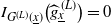 $I_{G^{(L)}(\underline{x})}\big(\widehat{g}_{\underline{x}}^{\, (L)}\big)=0$
. We can also say that
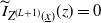 $\widetilde{I}_{Z^{(L+1)}(\underline{x})}(z)=0$
if and only if
 $z=0\in\mathbb{R}^{|A|\times n_{L+1}}$
.
Remark 2. The matrix
 $\widehat{g}_{\underline{x}}^{\, (\ell)}$
in (9) coincides with
 $K^{(\ell+1)}=\big(K_{\alpha\beta}^{(\ell+1)}\big)_{\alpha,\beta\in A}$
in [Reference Hanin15, (1.7) and (1.8)].
Remark 3. If
 $|A|=1$
we simply have
 $\cal{S}_{|A|,C_b}=[C_b,\infty)$
and
 $x\in\mathbb{R}^{n_0}$
in place of
 $\underline{x}$
. Then, if we specialize (10) to this case, we get
 $$I_{Z^{(L+1)}(x)}(z) \, :\! = \, \inf_{g^{(L)}\geq C_b}\bigg\{I_{G^{(L)}(x)}\big(g^{(L)}\big) + \frac{\|z\|^2}{2g^{(L)}}\bigg\}, \quad z\in\mathbb{R}^{n_{L+1}}.$$
Note that we can have
 $g^{(L)}=0$
if
 $C_b=0$
and, if we consider the rule
 ${0}/{0}=0$
as usual, the argument of the infimum above computed at
 $g^{(L)}=0$
is
 $$\bigg\{I_{G^{(L)}(x)}\big(g^{(L)}\big) + \frac{\|z\|^2}{2g^{(L)}}\bigg\}\bigg|_{g^{(L)}=0} = \begin{cases} I_{G^{(L)}(x)}(0) & \mbox{if}\ z=0, \\ \infty & \mbox{if}\ z\neq 0. \end{cases}$$
Moreover, we have
 $\widehat{g}_x^{(L)}\geq C_b\geq 0$
, and (13) yields
 $$\widetilde{I}_{Z^{(L+1)}(x)}(z) \, :\! = \, \frac{\|z\|^2}{2\widehat{g}_x^{(L)}}, \quad z\in\mathbb{R}^{n_{L+1}}.$$
Finally, we also remark that if
 $|A|=1$
and
 $\widehat{g}_x^{(L)}=0\in\mathbb{R}$
(this can happen if
 $C_b=0$
), we have
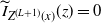 $\widetilde{I}_{Z^{(L+1)}(x)}(z)=0$
if
 $z=0\in\mathbb{R}^{n_{L+1}}$
, and
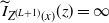 $\widetilde{I}_{Z^{(L+1)}(x)}(z)=\infty$
otherwise.
3. Proofs of the main results
In this section we recall some preliminaries on large deviations (basic definitions and results), we provide an important representation lemma, and we present the proofs of Theorems 1 and 2.
3.1. Preliminaries on large deviations
We start with the basic definition of an LDP (see, e.g., [Reference Dembo and Zeitouni9]), and other related concepts. In view of what follows we present these definitions by referring to sequences of probability measures.
Definition 1. A sequence of positive numbers
 $\{v_n\colon n\geq 1\}$
such that
 $v_n\to\infty$
(as
 $n\to\infty$
) is called a speed function, and a lower semicontinuous function
 $I\colon\cal{X}\to[0,\infty]$
is called a rate function. Let
 $\cal{X}$
be a topological space, and let
 $\{\pi_n\}_n$
be a sequence of probability measures on
 $\cal{X}$
(equipped with its completed Borel
 $\sigma$
-field). Then
 $\{\pi_n\}_n$
satisfies the large-deviation principle on
 $\cal{X}$
with speed
 $v_n$
and rate function I if
 \begin{align*} \limsup_{n\to\infty}\frac{1}{v_n}\log\pi_n(C) & \leq -\inf_{x\in C}I(x) \quad \textrm{for all closed sets} \, \textit{C},{\textit {and}} \\ \liminf_{n\to\infty}\frac{1}{v_n}\log\pi_n(O) & \geq -\inf_{x\in O}I(x) \quad \textrm{for all open sets} \, \textit{O}. \end{align*}
Moreover, the rate function I is said to be good if, for every
 $\unicode{x03BB}\geq 0$
, the level set
 $\{x\in\mathbb{R}\colon I(x)\leq\unicode{x03BB}\}$
is compact. If the above upper bound holds for compact sets only, then we say that
 $\{\pi_n\}_n$
satisfies the weak large-deviation principle (WLDP) on
 $\cal{X}$
.
The results in this paper are stated for sequences of random variables
 $\{R_n\}_n$
, say, defined on the same probability space
 $(\Omega,\cal{F},P)$
, and taking values on the same topological space
 $\cal{X}$
. Indeed, we refer to the sequence of laws, i.e. to the framework of the above definition with
 $\pi_n=P(R_n\in\cdot)$
.
Throughout this paper we refer to some well-known large-deviation results: the Gärtner–Ellis theorem (see, e.g., [Reference Dembo and Zeitouni9, Theorem 2.3.6(c)]), and the contraction principle (see, e.g., [Reference Dembo and Zeitouni9, Theorem 4.2.1]). We also refer to the concept of an essentially smooth function (see, e.g., [Reference Dembo and Zeitouni9, Definition 2.3.5]).
An important result used in this paper is [Reference Chaganty8, Theorem 2.3]. We recall its statement here.
Proposition 1. Let
 $\Omega_1$
and
 $\Omega_2$
be two Polish spaces. Let
 $\{\pi_n\colon n\geq 1\}$
be a sequence of probability measures on
 $\cal{X}=\Omega_1\times\Omega_2$
, and denote the sequences of marginal distributions by
 $\{\pi_{1,n}\colon n\geq 1\}$
on
 $\Omega_1$
and
 $\{\pi_{2,n}\colon n\geq 1\}$
on
 $\Omega_2$
. We assume that the following conditions hold.
-
(i) The sequence
$\{\pi_{1,n}\colon n\geq 1\}$
satisfies the LDP on
$\Omega_1$
with speed
$v_n$
and good rate function
$I_1$
. -
(ii) If
$\{x_{1,n}\colon n\geq 1\}\subset\Omega_1$
and
$x_{1,n}\to x_1\in\Omega_1$
, then the sequence of conditional distributions
$\big\{\pi_n^{2|1}(dx_2\mid x_{1,n})\colon n\geq 1\big\}$
satisfies the LDP on
$\Omega_2$
with speed
$v_n$
and rate function
$J(\cdot\mid x_1)$
. -
(iii)
$(x_1,x_2)\mapsto J(x_2\mid x_1)$
is lower semicontinuous.








Then
 $\{\pi_n\colon n\geq 1\}$
satisfies the WLDP on
 $\Omega_1\times\Omega_2$
with speed
 $v_n$
and rate function I defined by
 $I(x_1,x_2) \, :\! = \,J(x_2\mid x_1)+I_1(x_1)$
. Moreover,
 $\{\pi_{2,n}\colon n\geq 1\}$
satisfies the LDP on
 $\Omega_2$
with speed
 $v_n$
and rate function
 $I_2$
defined by
 $$I_2(x_2) \, :\! = \,\inf_{x_1\in\Omega_1}\{I(x_1,x_2)\} = \inf_{x_1\in\Omega_1}\{J(x_2\mid x_1)+I_1(x_1)\};$$
 $\{\pi_n\colon n\geq 1\}$
satisfies the LDP on
 $\Omega_1\times\Omega_2$
if the rate function I is good and, in such a case, the rate function
 $I_2$
is also good.
We also recall another useful related result (for its proof, see [Reference Chaganty8, Lemma 2.6]).
Lemma 1. Consider the same hypotheses and notation as Proposition 1. Assume that, for every
 $a\geq 0$
and for every compact subset
 $K_1$
of
 $\Omega_1$
, the set
 $\bigcup_{x_1\in K_1}\{x_2\in\Omega_2\colon J(x_2\mid x_1)\leq a\}$
is a compact subset of
 $\Omega_2$
. Then the rate function I in Proposition 1 is good.
We conclude this section with a useful lemma. We consider a Polish space
 $\Pi$
and, for any given
 $\bar{r}\in\Pi$
, let
 $\Delta(\cdot \! ;\, \bar{r})\colon \Pi\to[0,\infty]$
be the function defined by
 $$\Delta(r;\, \bar{r}) \, :\! = \, \begin{cases} 0 & \mbox{if}\ r=\bar{r}, \\ \infty & \mbox{if}\ r\neq\bar{r}. \end{cases}$$
In particular, we remark that
 $\Delta(\cdot \! ;\, \bar{r})$
is trivially a good rate function; indeed, every level set is compact because
 $\{r\in\mathbb{R}\colon\Delta(r;\,\bar{r})\leq a\}=\{\bar{r}\}$
for all
 $a\geq 0$
. In what follows, we consider this function with
 $\Pi=\cal{S}_{|A|,C_b}\subset\mathbb{R}^{|A|\times|A|}$
.
Lemma 2 ([Reference Giuliano, Macci and Pacchiarotti13, Lemma 1].) Let
 $\{\psi_n\}_n$
be a sequence of probability measures on some Polish space
 $\Pi$
that satisfies the LDP with speed
 $s_n$
and good rate function H, which uniquely vanishes at some
 $r_0$
. Moreover, let
 $t_n$
be another speed function such that
 ${s_n}/{t_n}\to\infty$
. Then
 $\{\psi_n\}_n$
satisfies the LDP with speed
 $t_n$
and good rate function
 $\Delta(\cdot \! ;\,r_0)$
.
3.2. An important representation lemma
The proofs of the main results are based on a different representation of the model. Such a representation is based on a recursive approach described without any mathematical details in [Reference Hanin15, Section 1.4, (1.9) and (1.10)]. Roughly speaking, we can say that the output of the network (layer
 $L+1$
) is centered multivariate normal distributed, with a random covariance matrix that depends on the random variables involved in the previous layers.
The aim of this section is to present a lemma with the mathematical details of the recursive approach described in [Reference Hanin15]. This representation holds for some fixed choices of
 $n_1,\ldots,n_L$
; however, for the future use of this lemma we write
 $n_1(n),\ldots,n_L(n)$
in place of
 $n_1,\ldots,n_L$
as in most of the rest of the paper.
Lemma 3. Let
 $\big\{N_{j\alpha}^{(\ell)}\colon j,\ell\geq 1,\alpha\in A\big\}$
be a family of independent standard normal-distributed random variables, and let
 $\big\{G_n^{(\ell)}(\underline{x})\colon n,\ell\geq 1\big\}$
be the
 $\cal{S}_{|A|,C_b}$
-valued random variables defined (by recurrence on
 $\ell\geq 1$
) by
 $G_n^{(\ell)}(\underline{x}) \, :\! = \,\big(G_{n;\,\alpha\beta}^{(\ell)}(\underline{x})\big)_{\alpha,\beta\in A}$
, where
 \begin{equation} G_{n;\,\alpha\beta}^{(\ell)}(\underline{x}) \, :\! = \, C_b + \frac{C_W}{n_\ell(n)}\sum_{j=1}^{n_\ell(n)} \sigma\big(\big\langle G_{n;\,\alpha\cdot}^{(\ell-1),\#}(\underline{x}),N_{j\cdot}^{(\ell)}\big\rangle\big)\sigma\big(\big\langle G_{n;\,\beta\cdot}^{(\ell-1),\#}(\underline{x}),N_{j\cdot}^{(\ell)}\big\rangle\big),\end{equation}
 $\big\langle G_{n;\,\gamma\cdot}^{(\ell-1),\#}(\underline{x}),N_{j\cdot}^{(\ell)}\big\rangle \, :\! = \, \sum_{\gamma^\prime\in A}G_{n;\,\gamma\gamma^\prime}^{(\ell-1),\#}(\underline{x}) N_{j\gamma^\prime}^{(\ell)}$
for every
 $\gamma\in A$
, and
 $G_n^{(0)}(\underline{x})=g^{(0)}(\underline{x})$
as in (8). Then, for
 $L\geq 1$
,
 $$ \big(Z_h^{(L+1)}(x_\alpha)\big)_{\alpha h} \stackrel{\mathrm{law}}{=} \Bigg(\sum_{\gamma\in A}G_{n;\,\alpha\gamma}^{(L),\#}(\underline{x})N_{h\gamma}^{(L+1)}\Bigg)_{\alpha h}. $$
Proof. Throughout this proof we simply write
 $n_\ell$
in place of
 $n_\ell(n)$
. Moreover, we can say that
 $\big\{G_n^{(\ell)}(\underline{x})\colon n,\ell\geq 1\big\}$
are
 $\cal{S}_{|A|,C_b}$
-valued random variables by construction. In what follows we prove the equality in law by induction on L, showing that the moment-generating functions (with argument
 $\theta\in\mathbb{R}^{|A|\times n_{L+1}}$
) coincide.
We start with the case
 $L=0$
, i.e.
 $$ \big(\big(Z_h^{(1)}(x_\alpha)\big)_{\alpha\in A}\big)_{h=1,\ldots,n_1} \stackrel{\mathrm{law}}{=} \Bigg(\Bigg(\sum_{\gamma\in A}G_{n;\,\alpha\gamma}^{(0),\#}(\underline{x}) N_{h\gamma}^{(1)}\Bigg)_{\alpha\in A}\Bigg)_{h=1,\ldots,n_1}, $$
where
 $G_n^{(0)}(\underline{x})=g^{(0)}(\underline{x})$
as in (8), and therefore
 $G_n^{(0),\#}(\underline{x})=g^{(0),\#}(\underline{x})$
. By (1) and some manipulations, we have
 \begin{multline*} \mathbb{E}\Bigg[\exp\Bigg(\sum_{\alpha\in A}\sum_{h=1}^{n_1}\theta_{\alpha h}Z_h^{(1)}(x_\alpha)\Bigg)\Bigg] \\\exp\Bigg(\frac{1}{2}\Bigg(C_b\sum_{h=1}^{n_1}\sum_{\alpha,\beta\in A}\theta_{\alpha h}\theta_{\beta h} + \frac{C_W}{n_0}\sum_{h=1}^{n_1}\sum_{r=1}^{n_0}\sum_{\alpha,\beta\in A} \theta_{\alpha h}\theta_{\beta h}x_{\alpha,r}x_{\beta,r}\Bigg)\Bigg).\end{multline*}
On the other hand, we also have (in the final equality we take into account (8))
 \begin{align*} & \mathbb{E}\Bigg[\exp\Bigg(\sum_{\alpha\in A}\sum_{h=1}^{n_1}\theta_{\alpha h} \sum_{\gamma\in A}G_{n;\,\alpha\gamma}^{(0),\#}(\underline{x})N_{h\gamma}^{(1)}\Bigg)\Bigg] \\& \qquad\qquad = \exp\Bigg(\frac{1}{2}\sum_{h=1}^{n_1}\sum_{\gamma\in A} \Bigg(\sum_{\alpha\in A}\theta_{\alpha h}g_{\alpha\gamma}^{(0),\#}(\underline{x})\Bigg)^2\Bigg) \\& \qquad\qquad = \exp\Bigg(\frac{1}{2}\sum_{h=1}^{n_1}\sum_{\alpha,\beta\in A} \theta_{\alpha h}\theta_{\beta h}g_{\alpha\beta}^{(0)}(\underline{x})\Bigg) \\ & \qquad\qquad = \exp\Bigg(\frac{1}{2}\sum_{h=1}^{n_1}\sum_{\alpha,\beta\in A}\theta_{\alpha h}\theta_{\beta h} \Bigg(C_b+\frac{C_W}{n_0}\sum_{r=1}^{n_0}x_{\alpha,r}x_{\beta,r}\Bigg)\Bigg). \end{align*}
So the case
 $L=0$
is proved.
Now we assume that the statement for L is proved, i.e.
 $$ \big(\big(Z_h^{(L)}(x_\alpha)\big)_{\alpha\in A}\big)_{h=1,\ldots,n_L} \stackrel{\mathrm{law}}{=} \Bigg(\Bigg(\sum_{\gamma\in A}G_{n;\,\alpha\gamma}^{(L-1),\#}(\underline{x})N_{h\gamma}^{(L)} \Bigg)_{\alpha\in A}\Bigg)_{h=1,\ldots,n_L}, $$
and we prove the statement for
 $L+1$
, i.e.
 $$ \big(\big(Z_h^{(L+1)}(x_\alpha)\big)_{\alpha\in A}\big)_{h=1,\ldots,n_{L+1}} \stackrel{\mathrm{law}}{=} \Bigg(\Bigg(\sum_{\gamma\in A}G_{n;\,\alpha\gamma}^{(L),\#}(\underline{x})N_{h\gamma}^{(L+1)} \Bigg)_{\alpha\in A}\Bigg)_{h=1,\ldots,n_{L+1}}. $$
By (1) and some manipulations, we have
 \begin{align*} & \mathbb{E}\Bigg[\exp\Bigg(\sum_{\alpha\in A}\sum_{h=1}^{n_{L+1}}\theta_{\alpha h}Z_h^{(L+1)}(x_\alpha)\Bigg)\Bigg] \\& \qquad = \mathbb{E}\Bigg[\exp\Bigg(\frac{C_b}{2}\sum_{h=1}^{n_{L+1}}\Bigg( \sum_{\alpha\in A}\theta_{\alpha h}\Bigg)^2\Bigg)\exp\Bigg(\frac{C_W}{2n_L}\sum_{h=1}^{n_{L+1}}\sum_{j=1}^{n_L}\Bigg( \sum_{\alpha\in A}\theta_{\alpha h}\sigma\big(Z_j^{(L)}(x_\alpha)\big)\Bigg)^2\Bigg)\Bigg] \nonumber\\[-2pt] & \qquad = \exp\Bigg(\frac{C_b}{2}\sum_{h=1}^{n_{L+1}}\sum_{\alpha,\beta\in A}\theta_{\alpha h}\theta_{\beta h}\Bigg) \\ & \qquad \quad \times \mathbb{E}\Bigg[\exp\Bigg(\frac{C_W}{2n_L} \sum_{h=1}^{n_{L+1}}\sum_{j=1}^{n_L}\sum_{\alpha,\beta\in A} \theta_{\alpha h}\theta_{\beta h}\sigma\big(Z_j^{(L)}(x_\alpha)\big)\sigma\big(Z_j^{(L)}(x_\beta)\big)\Bigg)\Bigg]; \end{align*}
thus, by some manipulations (in the first equality we take into account the inductive hypothesis, and in the second equality we take into account (14)), we obtain
 \begin{align*} & \mathbb{E}\Bigg[\exp\Bigg(\sum_{\alpha\in A}\sum_{h=1}^{n_{L+1}}\theta_{\alpha h}Z_h^{(L+1)}(x_\alpha)\Bigg)\Bigg] \\ & \qquad\qquad = \mathbb{E}\Bigg[\exp\Bigg(\frac{1}{2}\sum_{h=1}^{n_{L+1}}\sum_{\alpha,\beta\in A} \theta_{\alpha h}\theta_{\beta h}\Bigg(C_b + \frac{C_W}{n_L}\sum_{j=1}^{n_L}\sigma\Bigg( \sum_{\gamma\in A}G_{n;\,\alpha\gamma}^{(L-1),\#}(\underline{x})N_{j\gamma}^{(L)}\Bigg) \\ & \qquad\qquad\quad \times \sigma\Bigg( \sum_{\gamma\in A}G_{n;\,\beta\gamma}^{(L-1),\#}(\underline{x})N_{j\gamma}^{(L)}\Bigg)\Bigg)\Bigg)\Bigg] \\ & \qquad\qquad = \mathbb{E}\Bigg[\exp\Bigg(\frac{1}{2}\sum_{h=1}^{n_{L+1}}\sum_{\alpha,\beta\in A} \theta_{\alpha h}\theta_{\beta h}G_{n;\,\alpha\beta}^{(L)}(\underline{x})\Bigg)\Bigg].\end{align*}
On the other hand, we also have
 \begin{align*} \mathbb{E}\Bigg[\exp\Bigg(\sum_{\alpha\in A}\sum_{h=1}^{n_{L+1}}\theta_{\alpha h} \sum_{\gamma\in A}G_{n;\,\alpha\gamma}^{(L),\#}(\underline{x})N_{h\gamma}^{(L+1)}\Bigg)\Bigg]& = \mathbb{E}\Bigg[\exp\Bigg(\frac{1}{2}\sum_{h=1}^{n_{L+1}}\sum_{\gamma\in A}\Big(\sum_{\alpha\in A}\theta_{\alpha h} G_{n;\,\alpha\gamma}^{(L),\#}(\underline{x})\Big)^2\Big)\Bigg] \\& =\mathbb{E}\Bigg[\exp\Bigg(\frac{1}{2}\sum_{h=1}^{n_{L+1}}\sum_{\alpha,\beta\in A}\theta_{\alpha h}\theta_{\beta h} G_{n;\,\alpha\beta}^{(L)}(\underline{x})\Bigg)\Bigg].\end{align*}
The statement for
 $L+1$
is proved.
3.3. Proofs of the theorems
Proof of Theorem
1. We prove the theorem by induction on L. Moreover, by Lemma 3, we refer to the random variables
 $\big(\sum_{\gamma\in A}G_{n;\,\alpha\gamma}^{(L),\#}(\underline{x})N_{h\gamma}^{(L+1)}\big)_{\alpha h}$
in place of the random variables
 $\big(Z_h^{(L+1)}(x_\alpha)\big)_{\alpha h}$
.
Actually, we prove by induction on L that

which we denote by
 $(\! \bullet \!)$
. Indeed, if
 $(\! \bullet \!)$
holds, we can conclude as follows:
 $\big\{\big(N_{\alpha h}^{(L+1)}/\sqrt{v_n^*}\big)_{\alpha h}\big\}_n$
satisfies the LDP (on
 $\mathbb{R}^{|A|\times n_{L+1}}$
) with good rate function
 $V(r) \, :\! = \,{\|r\|^2}/{2}$
(this is a standard application of the Gärtner–Ellis theorem); therefore, by a simple application of the contraction principle, we get that the desired LDP holds with good rate function
 $I_{Z^{(L+1)}(\underline{x})}$
defined by (10) because the function
 $$ \big(g^{(L)},r\big) = \big(\big(g_{\alpha\beta}^{(L)}\big)_{\alpha,\beta\in A},(r_{\alpha h})_{\alpha h}\big) \mapsto g^{(L),\#}r = \Bigg(\sum_{\gamma\in A}g_{\alpha\gamma}^{(L),\#}r_{\gamma h}\Bigg)_{\alpha h} $$
is continuous (here we also take into account [Reference Bathia4, Theorem X.1.1]).
We start with the case
 $L=1$
. In this case the ratio
 ${n_\ell(n)}/{n_{\widehat{\ell}}(n)}$
in Condition 2 is trivially equal to 1 (because we have
 $\ell=\widehat{\ell}=1$
); thus
 $v_n^*=n_1(n)$
and
 $\gamma_L=\gamma_1=1<\infty$
. Firstly, it is easy to check that, by (14) with
 $\ell=1$
, for all
 $\eta\in\mathbb{R}^{|A|\times|A|}$
we have
 $$ \lim_{n\to\infty}\frac{1}{v_n^*}\log\mathbb{E}\big[ \exp\big\{v_n^*\big\langle\eta,G_n^{(1)}(\underline{x})\big\rangle\big\}\big] = \langle\eta,C_b\mathbf{1}\rangle + \kappa\big(C_W\eta; \, g^{(0)}(\underline{x})\big) =: \, \Psi\big(\eta; \, g^{(0)}(\underline{x})\big). $$
So, by the Gärtner–Ellis theorem on
 $\mathbb{R}^{|A|\times|A|}$
(note that
 $\Omega_2\subset\mathbb{R}^{|A|\times|A|}$
), we prove
 $(\! \bullet \!)$
for
 $L=1$
(so we necessarily have
 $\gamma_1=1$
) noting that, by (12) with
 $\gamma_1=1$
,
 $$ \sup_{\eta\in\mathbb{R}^{|A|\times|A|}}\big\{\big\langle\eta,g^{(1)}\big\rangle - \Psi\big(\eta;\,g^{(0)}(\underline{x})\big)\big\} = J\big(g^{(1)}\mid g^{(0)}(\underline{x})\big) $$
coincides with
 $I_{G^{(1)}(\underline{x})}\big(g^{(1)}\big)$
(see (11) for
 $L=1$
, with a slight abuse of notation; indeed, the infimum in (11) disappears because
 $g^{(1)}$
is fixed, we have the unique constraint
 $g^{(0)}=g^{(0)}(\underline{x})$
because the constraint
 $g^{(1)},\ldots,g^{(L-1)}\in\cal{S}_{|A|,C_b}$
is empty, and the sum in (11) is reduced to single summand). We also remark that
 $I_{G^{(1)}(\underline{x})}$
is a good rate function; indeed (here we restrict to the case
 $\gamma_1=1$
for what we have said above, but this restriction is not necessary), the function
 $\Psi\big(\cdot \! ;\, g^{(0)}(\underline{x})\big)$
assumes finite values because
 $\sigma(\! \cdot \!)$
is bounded (by Condition 1) and we can refer to [Reference Dembo and Zeitouni9, Lemma 2.2.20].
Now we consider the inductive hypothesis, i.e. we assume that
 $(\! \bullet \!)$
holds for
 $L-1$
(for
 $L\geq 2$
). In what follows we prove that
 $(\! \bullet \!)$
holds by a suitable application of Proposition 1 with
 $\Omega_1=\Omega_2=\cal{S}_{|A|,C_b}$
. So we have to check the following three items:
-
(i)
$I_{G^{(L)}(\underline{x})}$
is a good rate function; -
(ii) if we take
$g_n^{(L-1)}\to g^{(L-1)}$
as
$n\to\infty$
in
$\Omega_1$
, then the sequence of conditional distributions
$\big\{P\big(G_n^{(L)}(\underline{x})\in\cdot\mid G_n^{(L-1)}(\underline{x})=g_n^{(L-1)}\big)\big\}_n$
satisfies the LDP on
$\Omega_2$
with speed
$v_n^*$
and rate function
$J(\cdot\mid g^{(L-1)})$
defined by (12); -
(iii) the function
$\big(g^{(L-1)},g^{(L)}\big)\mapsto J\big(g^{(L)}\mid g^{(L-1)}\big)$
is lower semicontinuous.








Indeed, if these conditions hold, we have the equality
 $$ I_{G^{(L)}(\underline{x})}\big(g^{(L)}\big) \, :\! = \, \inf_{g^{(L-1)}\in\cal{S}_{|A|,C_b}}\big\{J\big(g^{(L)}\mid g^{(L-1)}\big) + I_{G^{(L-1)}(\underline{x})}\big(g^{(L-1)}\big)\big\}, $$
which meets the expression in (11).
We start with item (ii). If we prove it for
 $\gamma_L<\infty$
, then the proof for
 $\gamma_L=\infty$
is a consequence of applying Lemma 2 with
 $\{\psi_n\}_n=\big\{P\big(G_n^{(L)}(\underline{x})\in\cdot\mid G_n^{(L-1)}(\underline{x})=g_n^{(L-1)}\big)\big\}_n$
,
 $H=J\big(\cdot\mid g^{(L-1)}\big)$
in (12) which uniquely vanishes at
 $r_0=C_b\mathbf{1}+C_Wy\big(g^{(L-1)}\big)\in\cal{S}_{|A|,C_b}$
(here we refer to y(q) defined in (7)),
 $s_n=n_L(n)$
, and
 $t_n=v_n^*$
(note that
 ${s_n}/{t_n}={n_L(n)}/{v_n^*}\to\gamma_L=\infty$
). So, in what follows, we restrict our attention to the case
 $\gamma_L<\infty$
. We start by noting that, by Lemma 3 (and (14) in particular), for all
 $\eta\in\mathbb{R}^{|A|\times|A|}$
we have
 $$ \mathbb{E}\big[\exp\big\{\big\langle\eta,G_n^{(L)}(\underline{x})\big\rangle\big\}\mid G_n^{(L-1)}(\underline{x})=g_n^{(L-1)}\big] = \exp\bigg(\langle\eta,C_b\mathbf{1}\rangle + n_L(n)\kappa\bigg(\frac{C_W}{n_L(n)}\eta;\,g_n^{(L-1)}\bigg)\bigg); $$
then, by Condition 1 (indeed,
 $\kappa(\cdot \! ;\,\cdot)$
assumes finite values because
 $\sigma(\! \cdot \!)$
is bounded, and it is also a continuous function as discussed just after (5)), we get
 \begin{multline*} \lim_{n\to\infty}\frac{1}{v_n^*}\log\mathbb{E}\big[ \exp\big\{v_n^*\big\langle\eta,G_n^{(L)}(\underline{x})\big\rangle\big\}\mid G_n^{(L-1)}(\underline{x}) = g_n^{(L-1)}\big] \\ = \langle\eta,C_b\mathbf{1}\rangle + \gamma_L\kappa\bigg(\frac{C_W}{\gamma_L}\eta;\,g^{(L-1)}\bigg) =: \Psi\big(\eta;\,g^{(L-1)}\big). \end{multline*}
So, by the Gärtner–Ellis theorem on
 $\mathbb{R}^{|A|\times|A|}$
(note that
 $\Omega_2\subset\mathbb{R}^{|A|\times|A|}$
), we prove item (ii) for L with
 $\gamma_L<\infty$
, noting that, by (12),
 $$ \sup_{\eta\in\mathbb{R}^{|A|\times|A|}}\big\{\big\langle\eta,g^{(L)}\big\rangle - \Psi\big(\eta;\,g^{(L-1)}\big)\big\} = J\big(g^{(L)}\mid g^{(L-1)}\big). $$
In particular, we can say that
 $J\big(\cdot\mid g^{(L-1)}\big)$
is a good rate function, indeed
 $\Psi\big(\cdot \! ;\,g^{(L-1)}\big)$
assumes finite values because
 $\sigma(\! \cdot \!)$
is bounded (by Condition 1), and we can refer to [Reference Dembo and Zeitouni9, Lemma 2.2.20] as before.
For item (iii), we have to check that, if
 $\big(g_n^{(L-1)},g_n^{(L)}\big)\to\big(g^{(L-1)},g^{(L)}\big)$
as
 $n\to\infty$
in
 $\Omega_1\times\Omega_2$
, then
 \begin{equation} \liminf_{n\to\infty}J\big(g_n^{(L)}\mid g_n^{(L-1)}\big) \geq J\big(g^{(L)}\mid g^{(L-1)}\big). \end{equation}
In order to do that (in both cases
 $\gamma_L<\infty$
and
 $\gamma_L=\infty$
), we can check that, by (12), for all
 $\eta\in\mathbb{R}^{|A|\times|A|}$
, we have
 $J\big(g_n^{(L)}\mid g_n^{(L-1)}\big) \geq \big\langle\eta,g_n^{(L)}\big\rangle - \Psi\big(\eta;\, g_n^{(L-1)}\big)$
, where (here we take into account that, for the case
 $\gamma_L=\infty$
, the function in (12) is the Legendre transform of a suitable linear function of
 $\eta$
)
 $$ \Psi\big(\eta; \, g^{(L-1)}\big) \, :\! = \, \begin{cases} \langle\eta,C_b\mathbf{1}\rangle + \gamma_L\kappa\bigg(\dfrac{C_W}{\gamma_L}\eta;\, g^{(L-1)}\bigg) & \mbox{if}\ \gamma_L<\infty, \\[3mm] \big\langle\eta,C_b\mathbf{1} + C_Wy\big(g^{(L-1)}\big)\big\rangle & \mbox{if}\ \gamma_L=\infty \end{cases} $$
(actually, the definition of
 $\Psi\big(\eta;\, g^{(L-1)}\big)$
for
 $\gamma_L<\infty$
was already given when we checked item (ii)); then we can say that (15) holds by letting n go to infinity and taking the supremum with respect to
 $\eta$
.
We conclude with item (i). In what follows we do not distinguish the cases
 $\gamma_L<\infty$
and
 $\gamma_L=\infty$
. We refer to the final statement of Proposition 1 with
 $\Omega_1=\Omega_2=\cal{S}_{|A|,C_b}$
, and to the inductive hypothesis (
 $I_{G^{(L-1)}(\underline{x})}$
is a good rate function); then it suffices to show that
 $$\big(g^{(L-1)},g^{(L)}\big) \mapsto J\big(g^{(L)}\mid g^{(L-1)}\big) + I_{G^{(L-1)}(\underline{x})}\big(g^{(L-1)}\big)$$
is a good rate function (then we get the goodness of
 $I_{G^{(L)}(\underline{x})}$
by an application of the final statement of Proposition 1). Moreover, by Lemma 1, it is enough to show that, for every compact
 $K\subset\Omega_1$
and
 $a\geq 0$
,
 $$ \cal{U}_{K,a} \, :\! = \, \bigcup_{g^{(L-1)}\in K}\big\{g^{(L)}\in\Omega_2\colon J\big(g^{(L)}\mid g^{(L-1)}\big) \leq a\big\} $$
is a compact set of
 $\Omega_2$
. We take a sequence
 $\{g_n\}_n$
in
 $\cal{U}_{K,a}$
and we have to show that there exists a subsequence that converges to a point in
 $\cal{U}_{K,a}$
. Firstly, for every n, there exists
 $h_n\in K$
such that
 $J(g_n\mid h_n)\leq a$
. Then there exists a subsequence of
 $\{h_n\}_n$
(which we again call
 $\{h_n\}_n$
) that converges to some
 $\widehat{h}\in K$
(because K is compact); moreover, for the corresponding subsequence of
 $\{g_n\}_n$
(which we again call
 $\{g_n\}_n$
), we have
 $J(g_n\mid h_n) = \sup_{\eta\in\mathbb{R}^{|A|\times|A|}}\{\eta g_n-\Psi(\eta;\, h_n)\}$
.
We remark that, since
 $\sigma(\! \cdot \!)$
is bounded by Condition 1, we have
 $J(g\mid h)<\infty$
if
 $$C_b\leq g_{\alpha\beta}\leq C_b+C_W\|\sigma\|_\infty^2\quad (\mbox{for all}\ \alpha,\beta\in A)$$
for every
 $g=(g_{\alpha\beta})_{\alpha,\beta\in A}$
and h (in particular, see also (14)). Then, since
 $J(g_n\mid h_n)\leq a$
, if we consider the notation
 $g_n=(g_{n;\,\alpha\beta})_{\alpha,\beta\in A}$
, we have
 $$C_b\leq g_{n;\,\alpha\beta}\leq C_b+C_W\|\sigma\|_\infty^2\quad (\mbox{for all}\ \alpha,\beta\in A).$$
Thus, there exists a compact set
 $\widetilde{K}\subset\cal{S}_{|A|,C_b}$
(which does not depend on n) such that
 $g_n\in\widetilde{K}$
, so there exists a subsequence of
 $\{g_n\}_n$
(which we again call
 $\{g_n\}_n$
) that converges to some
 $\widehat{g}\in\widetilde{K}$
. In conclusion, by item (iii) above, we have
 $a\geq\liminf_{n\to\infty}J(g_n\mid h_n)\geq J\big(\widehat{g}\mid \widehat{h}\big)$
; thus
 $\widehat{g}\in\cal{U}_{K,a}$
because
 $\widehat{g}\in\{g\in\Omega_2\colon J\big(g\mid\widehat{h}\big)\leq a\}$
and
 $\widehat{h}\in K$
.
Remark 4. Actually, we can say that
 $\big\{\big(G_n^{(1)}(\underline{x}),\ldots,G_n^{(L)}(\underline{x})\big)\big\}_n$
satisfies the LDP on
 $(\cal{S}_{|A|,C_b})^L$
with speed
 $v_n^*$
and good rate function
 $I_{G^{(1:L)}(\underline{x})}\big(g^{(1)},\ldots,g^{(L)}\big) = \sum_{\ell=1}^LJ\big(g^{(\ell)}\mid g^{(\ell-1)}\big)$
, where
 $g^{(0)}=g^{(0)}(\underline{x})$
is defined by (8). This LDP yields the one stated in
 $(\! \bullet \!)$
.
Proof of Theorem
2. We follow the same lines as the proof of Theorem 1 (we refer again to Lemma 3). For every
 $L\geq 1$
we take into account statement
 $(\! \bullet \!)$
together with Lemma 2 with
 $\{\psi_n\}_n=\big\{P\big(G_n^{(L)}(\underline{x})\in\cdot\big)\big\}_n$
,
 $H=I_{G^{(L)}(\underline{x})}$
in (11), which uniquely vanishes at
 $r_0=\widehat{g}_{\underline{x}}^{\, (L)}$
,
 $s_n=v_n^*$
, and
 $t_n=1/a_n$
(note that
 ${s_n}/{t_n}=a_nv_n^*\to\infty$
). Then we have
 \begin{align*} & \big\{G_n^{(L)}(\underline{x})\big\}_n \text{ satisfies the LDP on } \cal{S}_{|A|,C_b} \text{ with speed } 1/a_n \\ & \text{and good rate function } \widetilde{I}_{G^{(L)}(\underline{x})}=\Delta\big(\cdot \! ;\,\widehat{g}_{\underline{x}}^{\, (L)}\big), \end{align*}
denoted by
 $(\bullet\bullet)$
. So, by
 $(\bullet\bullet)$
and by the LDP of
 $\big\{\big(\sqrt{a_n}N_{\alpha h}^{(L+1)}\big)_{\alpha h}\big\}_n$
(which can be obtained by a standard application of the Gärtner–Ellis theorem), a simple application of the contraction principle (already explained in the proof of Theorem 1) yields the desired LDP with rate function
 $$ \widetilde{I}_{Z^{(L+1)}(\underline{x})}(z) = \inf_{g^{(L)}\in\cal{S}_{|A|,C_b},r\in\mathbb{R}^{|A|\times n_{L+1}}} \bigg\{\Delta\big(g^{(L)};\, \widehat{g}_{\underline{x}}^{\, (L)}\big) + \frac{\|r\|^2}{2}\colon\widehat{g}^{\, (L),\#}r=z\bigg\} $$
(for
 $z\in\mathbb{R}^{|A|\times n_{L+1}}$
), which coincides with the rate function in (13).
4. Large and moderate deviations of deep neural networks with ReLU pre-activation and single input
In this section we assume that
 $|A|=1$
(as in Remark 3) and some notation can be simplified. In particular, for a standard normal random variable N, we have
 $$\kappa(\eta;\, q) \, :\! = \, \log\mathbb{E}\big[\exp\{\eta\sigma^2(\sqrt{q}N)\}\big]\quad(\eta\in\mathbb{R}),$$
where
 $q\in\cal{S}_{|A|,C_b}=[C_b,\infty)$
. Moreover we still consider the Legendre transform of
 $\kappa(\cdot \! ;\, q)$
in (6), i.e.
 $\kappa^*(y;\, q)=\sup_{\eta\in\mathbb{R}}\{\eta y-\kappa(\eta;\, q)\}$
.
In this section, motivated by the literature, we consider ReLU networks, i.e.
 $\sigma(x) \, :\! = \,\max\{x,0\}$
. In this case the function
 $\sigma(\! \cdot \!)$
is continuous and unbounded; therefore we cannot refer to Theorems 1 and 2. However, we can obtain the same results by considering suitable modifications of some parts of the proofs, which will be discussed in this section.
4.1. Modifications of the proofs of Theorems 1 and 2
The parts with
 $\gamma_L=\infty$
still work well (and therefore the proof of Theorem 2). On the other hand, when
 $\gamma_L<\infty$
, we have to change some parts in which we use the Gärtner–Ellis theorem in the proof of Theorem 1. For
 $q>0$
we have
 \begin{align*} \kappa(\eta;\, q) = \log\mathbb{E}\big[\exp\{\eta\sigma^2(\sqrt{q}N)\}\big] & = \log\mathbb{E}\big[\exp\big\{\eta qN^2\cdot 1_{\{N\geq 0\}}\big\}\big] \\ & = \log\big(\mathbb{E}\big[{\mathrm{e}}^{\eta qN^2}1_{\{N\geq 0\}}\big]+P(N<0)\big) \\ & = \log\bigg(\int_0^\infty{\mathrm{e}}^{\eta qx^2}\frac{{\mathrm{e}}^{-{x^2}/{2}}}{\sqrt{2\pi}}\,{\mathrm{d}} x + \frac12\bigg) \\ & = \log\bigg(\frac12\bigg(\int_{-\infty}^\infty{\mathrm{e}}^{\eta qx^2}\frac{{\mathrm{e}}^{-{x^2}/{2}}}{\sqrt{2\pi}}\,{\mathrm{d}} x + 1\bigg)\bigg) \\ & = \begin{cases} \log\big(\frac12({(1-2\eta q)^{-1/2}+1})\big) & \mbox{if}\ \eta<(2q)^{-1}, \\ \infty & \mbox{otherwise}. \end{cases} \end{align*}
Obviously, this formula also holds for
 $q=0$
(this can happen when
 $C_b=0$
), and we have
 $\kappa(\eta;\,0)=0$
for all
 $\eta\in\mathbb{R}$
. Then, for every
 $q\geq C_b$
,
 $\kappa(\eta;\, q)$
is finite in a neighborhood of the origin
 $\eta=0$
, essentially smooth, and lower semicontinuous (note that, under these conditions, the rate function
 $\kappa^*(\cdot \! ;\, q)$
is good by [Reference Dembo and Zeitouni9, Lemma 2.2.20]). Moreover, we need to have
 \begin{equation} \lim_{n\to\infty}\kappa(\eta_n;\,q_n) = \kappa(\eta;\, q)\quad \mbox{as}\ q_n\to q\geq C_b\ \mbox{and}\ \eta_n\to\eta\in\mathbb{R};\end{equation}
indeed, we can easily check this condition (it is useful to distinguish the cases
 $\eta<(2q)^{-1}$
,
 $\eta>(2q)^{-1}$
, and
 $\eta=(2q)^{-1}$
; if
 $q=0$
we always have
 $\eta<(2q)^{-1}$
). We remark that in the proofs of Theorems 1 and 2, the function
 $\sigma(\! \cdot \!)$
is bounded and condition (16) holds; indeed, in that case, we have a sequence of finite-valued functions, and the limit of this sequence is a finite-valued function.
Other modifications concern the details of how to check item (i) in the proof of Theorem 1. We recall that, taking into account that
 $|A|=1$
,
 $J(g\mid h)=\sup_{\eta\in\mathbb{R}}\{\eta g-\Psi(\eta;\,h)\}$
, where
 $$\Psi(\eta;\,h) \, :\! = \, \begin{cases} C_b\eta+\gamma_L\kappa\bigg(\dfrac{C_W}{\gamma_L}\eta;\,h\bigg) & \mbox{if}\ \gamma_L<\infty, \\[3mm] (C_b+C_Wy(h))\eta & \mbox{if}\ \gamma_L=\infty.\end{cases} $$
We follow the same lines as that part of the proof of Theorem 1: for a compact subset K of
 $[C_b,\infty)$
, we have
 $h_n\in K$
for every n, and
 $J(g_n\mid h_n)\leq a$
; then we have to check that there exists a subsequence of
 $\{g_n\}_n$
(which we again call
 $\{g_n\}_n$
) that belongs to a compact subset
 $\widetilde{K}$
(say) of
 $[C_b,\infty)$
. The case
 $\gamma_L=\infty$
is trivial because, for a standard normal-distributed random variable N, we have
 $J(g_n\mid h_n)\leq a$
if and only if
 $$g_n=C_b+C_Wy(h_n)=C_b+C_W\mathbb{E}\big[(\max\{\sqrt{h_n}N,0\})^2\big]=C_b+C_Wh_n\mathbb{E}[N^21_{N\geq 0}].$$
So, in what follows, we discuss the case
 $\gamma_L<\infty$
. If
 $h=0$
(this can happen if
 $C_b=0$
) we have
 $\kappa(\eta;\,0)=0$
for all
 $\eta\in\mathbb{R}$
and
 $J(g\mid0)=\sup_{\eta\in\mathbb{R}}\{\eta (g-C_b)\}=\Delta(g;\,C_b)$
; if
 $h>0$
we have
 $\kappa(\eta;\, q)=\kappa(\eta q;\,1)$
and
 \begin{align*} J(g\mid h) & = \sup_{\eta\in\mathbb{R}}\big\{\eta g-\big(C_b\eta+\gamma_L\kappa(C_W\eta/\gamma_L;\,h)\big)\big\} \\ & = \sup_{\eta\in\mathbb{R}}\big\{\eta(g-C_b)-\gamma_L\kappa(C_W\eta h/\gamma_L;\,1)\big\} \\& = \sup_{\eta\in\mathbb{R}}\big\{\eta((g-C_b)/h+C_b)-(C_b\eta+\gamma_L\kappa(C_W\eta/\gamma_L;\,1))\big\} \\ & = J((g-C_b)/h+C_b;\,1).\end{align*}
Then
 $J(g_n\mid h_n)\leq a$
yields
 $({g_n-C_b})/{h_n}+C_b\in\{y\in\mathbb{R}\colon J(y\mid1)\leq a\}$
if
 $h_n>0$
(and
 $\{y\in\mathbb{R}\colon J(y\mid1)\leq a\}$
is a compact set that does not depend on n), and
 $g_n=C_b$
if
 $h_n=0$
; thus (here we do not distinguish the cases
 $h_n>0$
and
 $h_n=0$
) there exists
 $M\geq C_b$
such that
 $$C_b\leq g_n\leq (M-C_b)h_n+C_b.$$
So
 $g_n$
belongs to a suitable compact subset
 $\widetilde{K}$
because
 $h_n$
belongs to a compact subset K. Then we can conclude as for the case in which
 $\sigma$
is bounded and continuous.
4.2. An explicit expression for
$\kappa^*(\cdot \! ;\, q)$

Let
 $\kappa^\prime(\eta;\, q)$
be the derivative with respect to
 $\eta$
, i.e.
 $$\kappa^\prime(\eta;\, q)=\frac{q(1-2\eta q)^{-3/2}}{(1-2\eta q)^{-1/2}+1},$$
and let
 $\eta=\eta_{y,q}$
be the unique solution of
 $\kappa^\prime(\eta;\, q)=y$
. Then we have
 $$\kappa^*(y;\, q)= \begin{cases} \eta_{y,q}y-\kappa(\eta_{y,q};\, q) & \mbox{if}\ y>0, \\ -\lim_{\eta\to-\infty}\kappa(\eta;\, q)=\log 2 & \mbox{if}\ y=0, \\ \infty & \mbox{if}\ y<0. \end{cases} $$
Moreover, if we consider the function
 $f(z)={z^3}/({z+1})$
(for
 $z>0$
), and we denote its inverse by
 $f^\leftarrow$
, then we have
 $(1-2\eta_{y,q}q)^{-1/2}=f^\leftarrow(y/q)$
, which yields
 $\eta_{y,q}=({1-(f^\leftarrow(y/q))^{-2}})/{2q}$
. Thus, for
 $y>0$
we have
 $$\kappa^*(y;\, q)=\frac{1-(f^\leftarrow(y/q))^{-2}}{2q}y-\log\frac{f^\leftarrow(y/q)+1}{2}.$$
Finally, we remark that it is possible to give an explicit expression for
 $f^\leftarrow(y/q)$
in terms of Cardano’s formula for cubic equations. So we have an explicit expression for
 $\kappa^*(y;\, q)$
for which in general only a variational formula is available.
5. Results for shallow neural networks and their sensitivities
In this section we consider shallow Gaussian neural networks, i.e. the model (1) with
 $L=1$
. We already remarked that in such a case, Condition 2 always holds. Throughout this section we set
 $n_1(n)=n$
, so that
 $v_n^*=n$
; then we have
 $$Z_h^{(2)}(x) = b_h^{(2)} + \frac{1}{\sqrt{n}\,}\sum_{j=1}^n\sqrt{C_W}\widehat{W}_{hj}^{(2)}\sigma\Bigg(b_j^{(1)}+\sum_{r=1}^{n_0}W_{jr}^{(1)}x_r\Bigg),\quad h=1,\ldots,n_2,$$
where the random variables
 $\widehat{W}_{ij}^{(2)}$
are standard normal distributed. We remark that we have a sum of n independent and identically distributed (i.i.d.) random variables (with respect to j) that depend on
 $h=1,\ldots,n_2$
and
 $x\in T\subset\mathbb{R}^{n_0}$
; this particular feature allows us to establish more results than those presented in the previous sections. In particular, motivated by the interest in the sensitivities with respect to the input
 $x\in T$
(see, e.g., [Reference Favaro, Hanin, Marinucci, Nourdin and Peccati12]), we can present results for some derivatives.
The aim of this section is to study large and moderate deviations of the
 $\mathbb{R}^{|A|\times n_2}$
-valued sequence of random variables (in the derivatives below we have
 $x=(x_1,\ldots,x_{n_0})$
)
 \begin{equation} \bigg\{\bigg(\frac1{\sqrt{n}\,}\frac{\partial^{s_h} Z_h^{(2)}(x)}{\partial x_1^{s_h}} \bigg|_{x=x_\alpha}\bigg)_{\alpha h}\bigg\}_n.\end{equation}
Here we assume a finite set of inputs (i.e.
 $T=\{x_\alpha\}_{\alpha\in A}$
for a finite set A) and we take
 $s_h\in\{0,1\}$
,
 $h=1,\ldots,n_2$
; so, in particular, we define
 ${\partial^{0} Z_h^{(2)}(x)}/{\partial x_1^{0}} \, :\! = \,Z_h^{(2)}(x)$
. Moreover, except for the case
 $s_1=\cdots=s_{n_2}=0$
, we assume that
 $\sigma$
is, almost everywhere, differentiable; instead, if all the
 $s_h$
are equal to 0,
 $\sigma$
may not be continuous.
It is easy to check that (17) reads
 $$\Bigg\{\Bigg(\frac{b_h^{(2)}}{\sqrt{n}\,}1_{\{s_h=0\}}+\frac{1}{n}\sum_{j=1}^nF_{hj}(x_\alpha)\Bigg)_{\alpha h}\Bigg\}_n,$$
where, for
 $x\in\mathbb{R}^{n_0}$
,
 \begin{equation*} F_{hj}(x) \, :\! = \,\sqrt{C_W}\widehat{W}_{hj}^{(2)} \sigma^{(s_h)}\Bigg(b_j^{(1)}+\sum_{r=1}^{n_0}W_{jr}^{(1)}x_{r}\Bigg) \big(W_{j1}^{(1)}\big)^{s_h}\quad \mbox{for}\ j=1,\ldots,n\end{equation*}
are n i.i.d.
 $\mathbb{R}$
-valued random variables.
In view of Propositions 2 and 3 (which follow), it is useful to introduce the following functions:
 $$\cal{I}_h(y_h) \, :\! = \, \begin{cases} {y_h^2}/{2C_b} & \mbox{if}\ C_b\neq 0\ \mbox{and}\ s_h=0, \\ \Delta(y_h;\,0) & \mbox{otherwise}\end{cases} $$
(for
 $h=1,\ldots,n_2$
and
 $y_h\in\mathbb{R}$
);

and
 \begin{align*} \widetilde{\Upsilon}(\theta;\,\underline{x}) & \, :\! = \, \frac{1}{2}\sum_{\alpha,\beta\in \, A}\sum_{h_1,h_2=1}^{n_2} \frac{\partial^2\Upsilon(\theta;\,\underline{x})}{\partial\theta_{\alpha h_1}\partial\theta_{\beta h_2}} \bigg|_{\theta=0} \theta_{\alpha h_1}\theta_{\beta h_2} \\ & = \frac{1}{2}\sum_{\alpha,\beta\in \, A}\sum_{h=1}^{n_2}C_W\mathbb{E}\Bigg[ \sigma^{(s_{h})}\Bigg(\sum_{r=1}^{n_0}W_{1r}^{(1)}x_{\alpha,r}\Bigg) \sigma^{(s_{h})}\Bigg(\sum_{r=1}^{n_0}W_{1r}^{(1)}x_{\beta,r}\Bigg)\big(W_{11}^{(1)}\big)^{2s_h}\Bigg] \theta_{\alpha h}\theta_{\beta h}\end{align*}
(for
 $\theta=(\theta_{\alpha h})_{\alpha\in A,h=1,\ldots,n_2}\in\mathbb{R}^{|A|\times n_2}$
).
Proposition 2. Assume that the function
 $\Upsilon(\theta;\,\underline{x})$
is finite in a neighborhood of the origin
 $\theta=0\in\mathbb{R}^{|A|\times n_2}$
. Then the sequence
 $$ \bigg\{\bigg(\frac{1}{\sqrt{n}\,}\frac{\partial^{s_h} Z_h^{(2)}(x)} {\partial x_1^{s_h}}\bigg|_{x=x_\alpha}\bigg)_{\alpha h}\bigg\}_n $$
satisfies the LDP on
 $\mathbb{R}^{|A|\times n_2}$
with speed n and good rate function
 $$ I_{\partial Z^{(2)}(\underline{x})}(z) \, :\! = \, \inf\Bigg\{\sum_{h=1}^{n_2}\cal{I}_h(y_h) + \Upsilon^*(f;\,\underline{x})\colon y_h+f_{\alpha h}=z_{\alpha h}\ \mbox{for}\ (\alpha,h)\in A\times\{1,\ldots,n_2\}\Bigg\}, $$
where
 $\Upsilon^*(f;\,\underline{x}) \, :\! = \,\sup_{\theta\in\mathbb{R}^{|A|\times n_2}}\big\{\sum_{\alpha\in A}\sum_{h=1}^{n_2} f_{\alpha h}\theta_{\alpha h}-\Upsilon(\theta;\,\underline{x})\big\}$
.
Proof. The result can be proved by combining the LDP of
 $\big\{\big({b_h^{(2)}}/{\sqrt{n}}\big)_h\big\}_n$
on
 $\mathbb{R}^{n_2}$
with speed n and good rate function
 $\sum_{h=1}^{n_2}\cal{I}_h(y_h)$
(this follows from a standard application of the Gärtner–Ellis theorem, and the independence of
 $b_1^{(2)},\ldots,b_{n_2}^{(2)}$
); the LDP of
 $\big\{\big(({1}/{n})\sum_{j=1}^nF_{hj}(x_\alpha)\big)_{(\alpha,h)}\big\}_n$
on
 $\mathbb{R}^{|A|\times n_2}$
with speed n and good rate function
 $\Upsilon^*(f;\,\underline{x})$
(by Cramér’s theorem; see, e.g., [Reference Dembo and Zeitouni9, Theorem 2.2.30 and the subsequent Remark (a)]); and a suitable application of the contraction principle (because the function
 $((y_h)_h,(f_{\alpha h})_{(\alpha,h)})\mapsto (y_h+f_{\alpha h})_{(\alpha,h)}$
is continuous).
Proposition 3. Assume that the function
 $\Upsilon(\theta;\,\underline{x})$
is finite in a neighborhood of the origin
 $\theta=0\in\mathbb{R}^{|A|\times n_2}$
. Then, for every sequence of positive numbers
 $\{a_n\}_n$
such that (3) holds with
 $v_n^*=n$
, the sequence
 $$ \bigg\{\bigg(\sqrt{a_n}\frac{\partial^{s_h} Z_h^{(2)}(x)}{\partial x_1^{s_h}} \bigg|_{x=x_\alpha}\bigg)_{\alpha h}\bigg\}_n $$
satisfies the LDP on
 $\mathbb{R}^{|A|\times n_2}$
with speed
 $1/a_n$
and good rate function
 $$ \widetilde{I}_{\partial Z^{(2)}(\underline{x})}(z) \, :\! = \, \inf\Bigg\{\sum_{h=1}^{n_2}\cal{I}_h(y_h) + \widetilde{\Upsilon}^*(f;\,\underline{x})\colon y_h+f_{\alpha h}=z_{\alpha h}\ \mbox{for}\ (\alpha,h)\in A\times\{1,\ldots,n_2\}\Bigg\}, $$
where
 $\widetilde{\Upsilon}^*(f;\,\underline{x}) \, :\! = \, \sup_{\theta\in\mathbb{R}^{|A|\times n_2}}\big\{\sum_{\alpha\in A}\sum_{h=1}^{n_2} f_{\alpha h}\theta_{\alpha h}-\widetilde{\Upsilon}(\theta;\,\underline{x})\big\}$
.
Proof. This is similar to the proof of the previous proposition. The result can be proved by combining the LDP of
 $\big\{\big(\sqrt{a_n}b_h^{(2)}\big)_h\big\}_n$
on
 $\mathbb{R}^{n_2}$
with speed
 $1/a_n$
and good rate function
 $\sum_{h=1}^{n_2}\cal{I}_h(y_h)$
; the LDP of
 $\big\{\big((n/a_n)^{-1/2}\sum_{j=1}^nF_{hj}(x_\alpha)\big)_{(\alpha,h)}\big\}_n$
on
 $\mathbb{R}^{|A|\times n_2}$
with speed
 $1/a_n$
and good rate function
 $\widetilde{\Upsilon}^*(f;\,\underline{x})$
(by [Reference Dembo and Zeitouni9, Theorem 3.7.1]); and the same application of the contraction principle as in the proof of Proposition 2.
Thus it is important to find conditions on
 $\sigma$
under which the function
 $\Upsilon(\cdot \! ;\,\underline{x})$
is finite in a neighborhood of the origin. For this purpose we present the following proposition.
Proposition 4. Assume that there exists
 $M>0$
such that
 \begin{equation} \max_{h=1,\ldots,n_2}\Bigg|\sigma^{(s_h)}\Bigg(b+\sum_{r=1}^{n_0}w_rx_{\alpha,r}\Bigg)w_1^{s_h}\Bigg| \leq M\Bigg(1+\Bigg|b+\sum_{r=1}^{n_0}w_rx_{\alpha,r}\Bigg|\Bigg) \end{equation}
for
 $s_h\in\{0,1\}$
,
 $\alpha\in A$
, and for every
 $b,w_1,\ldots,w_{n_0}\in\mathbb{R}$
. Then
 $\Upsilon(\cdot \! ;\,\underline{x})$
is finite in a neighborhood of the origin.
Proof. It is easy to check (by taking into account (18)) that, for some
 $C>0$
, we have
 $$ \sum_{h=1}^{n_2}\Bigg(\sum_{\alpha\in A}\theta_{\alpha h} \sigma^{(s_h)}\Bigg(b+\sum_{r=1}^{n_0}w_rx_{\alpha,r}\Bigg) w_1^{s_h}\Bigg)^2 \leq C\sum_{h=1}^{n_2}\sum_{\alpha\in A}\theta_{\alpha h}^2 \Bigg(1+b^{2}+\sum_{r=1}^{n_0}w_r^{2}\Bigg); $$
thus
 \begin{align*} \Upsilon(\theta;\,\underline{x}) & = \log\mathbb{E}\Bigg[\exp\Bigg(\frac{C_W}{2}\sum_{h=1}^{n_2}\Bigg(\sum_{\alpha\in A}\theta_{\alpha h} \sigma^{(s_h)}\Bigg(b_1^{(1)}+\sum_{r=1}^{n_0}W_{1r}^{(1)}x_{\alpha,r}\Bigg) \big(W_{11}^{(1)}\big)^{s_h}\Bigg)^2\Bigg)\Bigg] \\ & \leq \log\mathbb{E}\Bigg[\exp\Bigg(C\sum_{h=1}^{n_2}\sum_{\alpha\in A}\theta_{\alpha h}^2 \Bigg(1+\big(b_1^{(1)}\big)^2+\sum_{r=1}^{n_0}\big(W_{1r}^{(1)}\big)^{2}\Bigg)\Bigg)\Bigg], \end{align*}
and the final expression is finite in a neighborhood of the origin since the random variables
 $b_1^{(1)}$
and
 $W_{1r}^{(1)}$
for
 $r=1,\ldots, n_0$
are Gaussian distributed and independent.
We could try to consider a stronger version of (18) referring to derivatives of order higher than the first one. In such a case we would have products of more than two independent Gaussian random variables, and it would not be possible to have a finite function
 $\Upsilon(\cdot \! ;\,\underline{x})$
in a neighborhood of the origin. In our opinion it would be possible to overcome this problem by considering a simplified model (for instance the case
 $C_b=0$
).
We conclude with some examples.
Example 1. If we take
 $s_1=\cdots=s_{n_2}=0$
then condition (18) is the sublinearity condition on
 $\sigma$
, i.e. there exists
 $C>0$
such that
 \begin{equation} |\sigma(x)|\leq C(1+|x|). \end{equation}
This condition holds, for instance, for every bounded function
 $\sigma$
(but, if
 $\sigma$
is also continuous, we can refer to the results in this paper with
 $L\geq 1$
), the function
 $\sigma(x)=\max\{x,0\}$
(already studied in Sectio 4) concerning ReLU networks, and the SWISH function
 $\sigma(x)={x}/({1+{\mathrm{e}}^{-x}})$
.
Example 2. We take
 $s_1=s_2=\cdots=s_{n_2}=1$
and we assume that the almost everywhere first derivative
 $\sigma^\prime$
is bounded, with essential supremum
 $\|\sigma^\prime\|_\infty$
. This condition holds for
 $\sigma(x)=\sin x$
, the sigmoid function
 $\sigma(x)={1}/({1+{\mathrm{e}}^{-x}})$
, the softplus function
 $\sigma(x)=\log(1+{\mathrm{e}}^{-x})$
, and we can still take the functions
 $\sigma(x)=\max\{x,0\}$
and
 $\sigma(x)={x}/({1+{\mathrm{e}}^{-x}})$
as in the previous example.


Acknowledgements
The authors thank two anonymous referees for their careful reading of the manuscript and for some useful comments.
Funding Information
All the authors acknowledge the support of Indam-GNAMPA. C.M. and B.P. acknowledge the support of the MUR Excellence Department Project awarded to the Department of Mathematics, University of Rome Tor Vergata (CUP E83C23000330006) and the support of the University of Rome Tor Vergata (project ‘Asymptotic Properties in Probability’ (CUP E83C22001780005)).
Competing Interests
There were no competing interests to declare which arose during the preparation or publication process of this article.



