





1. Introduction
Velocity fluctuations within a turbulent fluid may hold small particles aloft long enough to transport them long distances. The resulting flows drive particulate transport within the oceans and atmosphere, forming a key part of the global sediment cycle and underpinning natural phenomena such as underwater turbidity currents (Meiburg & Kneller Reference Meiburg and Kneller2010), river suspensions (Martinelli et al. Reference Martinelli, Victoria, Devol, Richey and Forsberg1989) and the atmospheric dispersion of dust and other pollutants (Bursik & Woods Reference Bursik and Woods1996; Schepanski Reference Schepanski2018). Consequently, the problem of understanding and modelling sediment transport by turbulence impinges upon many topics of practical interest in science and engineering (Dyer & Soulsby Reference Dyer and Soulsby1988; Elfrink & Baldock Reference Elfrink and Baldock2002; Gislason, Oelkers & Snorrason Reference Gislason, Oelkers and Snorrason2006; Dethier, Renshaw & Magilligan Reference Dethier, Renshaw and Magilligan2022). Since natural particles are typically denser than their carrier fluid, they preferentially concentrate in the direction of gravity, causing the local density of fluid–sediment parcels to increase towards the base of the flow. This stratifies the mixture and extracts energy from the turbulent eddies that support the suspension (Villaret & Trowbridge Reference Villaret and Trowbridge1991; Winterwerp Reference Winterwerp2001; Cantero et al. Reference Cantero, Balachandar, Cantelli, Pirmez and Parker2009a ; Huang et al. Reference Huang, Zhang, Zhang and Li2022). In some cases, this effect can be sufficient to fully or partially laminarise the flow, thereby collapsing the suspension (Cantero et al. Reference Cantero, Cantelli, Pirmez, Balachandar, Mohrig, Hickson, Yeh, Naruse and Parker2012a ; Shringarpure, Cantero & Balachandar Reference Shringarpure, Cantero and Balachandar2012).
The study of turbulent particle transport and the related phenomenon of stratified damping may be coarse grained by averaging over fluctuations within a particular flow – an approach that captures the most important global balances in the system (see, e.g. Garcia & Parker Reference Garcia and Parker1991; Fredsøe & Deigaard Reference Fredsøe and Deigaard1992; Wright & Parker Reference Wright and Parker2004). However, it is the aggregate effect of countless individual coherent motions within the flow that ultimately maintains a sediment suspension. Consequently, there exists a large body of research dedicated to observing, characterising and analysing discrete flow structures in the turbulent boundary layer (Kline et al. Reference Kline, Reynolds, Schraub and Runstadler1967; Corino & Brodkey Reference Corino and Brodkey1969; Robinson Reference Robinson1991) and assessing their role in mobilising and transporting sediment, which may be inferred via experimental measurements and computer simulations (Grass Reference Grass1971; Jackson Reference Jackson1976; Sumer & Oguz Reference Sumer and Oguz1978; Dyer & Soulsby Reference Dyer and Soulsby1988; Nelson et al. Reference Nelson, Shreve, McLean and Drake1995; Cellino & Lemmin Reference Cellino and Lemmin2004; Shringarpure et al. Reference Shringarpure, Cantero and Balachandar2012; Salinas et al. Reference Salinas, Balachandar and Cantero2021a , Reference Salinas, Balachandar, Shringarpure, Fedele, Hoyal, Zuñiga and Canterob ). In particular, studies have highlighted the central role that vortices play in ejecting particles upwards, away from the underlying boundary and into the bulk of the flow, thereby facilitating their transport downstream. Though it was proposed many years ago by Dyer & Soulsby (Reference Dyer and Soulsby1988) that knowledge of this mechanism could be used to improve upon the poor performance empirical sediment transport formulae, there has been scant progress in this direction to date.
It is within this context that we position the present contribution. However, rather than investigating sediment-laden turbulence directly (by, for example, measuring correlations between unsteady flow variables), we study a class of laminar vortex states (‘exact coherent structures’), which are invariant solutions of the Navier–Stokes equations coupled, in this case, with an equation that describes the motion of a dilute particle phase. The relevance of these flow states to turbulence stems from the fact that, when the governing equations are viewed as a dynamical system, they can lie embedded within the turbulent part of phase space, or along surfaces that separate laminar and turbulent conditions, and are only mildly unstable (in the sense of possessing a low number of unstable eigenmodes relative to the high dimensionality of the system). This means that during the course of a turbulent flow’s evolution it can make frequent, but transient, visits to these states, which locally guide the dynamics along their stable and unstable manifolds. This conceptual picture is clearest in small computational domains at transitionally turbulent Reynolds numbers, where these solutions have been most commonly studied (Gibson, Halcrow & Cvitanović Reference Gibson, Halcrow and Cvitanović2008; Cvitanović & Gibson Reference Cvitanović and Gibson2010). However, it is widely argued that unstable invariant solutions form the essential building blocks of more complex spatially extended flows, as well as underpinning the near-wall coherent motions that produce and regenerate turbulence (Kawahara & Kida Reference Kawahara and Kida2001; Waleffe Reference Waleffe2001; Itano & Generalis Reference Itano and Generalis2009; Kawahara et al. Reference Kawahara, Uhlmann and van Veen2012; Shekar & Graham Reference Shekar and Graham2018).
Given the mature state of the established theory for homogeneous flows, it is reasonable to expect that these states are necessary flow structures for supporting sediment suspensions, with properties that capture aspects of the turbulence itself. This is useful, since individual invariant solutions, being far simpler than a chaotic turbulent flow trajectory, are amenable to direct mathematical analysis (Hall & Sherwin Reference Hall and Sherwin2010; Deguchi & Hall Reference Deguchi and Hall2014). Furthermore, their vortical structure provides an exact analogue to the transient coherent structures that have long been observed to lift particles vertically and downstream in turbulent shear flows (Jackson Reference Jackson1976; Sumer & Oguz Reference Sumer and Oguz1978). Consequently, understanding their role, even in simple configurations, may be a necessary first step en route to improving sediment transport models which currently neglect flow structures in favour of bulk statistical averages.
However, despite over three decades of research on these states in a variety of canonical homogeneous flows, little is known about their interaction with sediment. Pestana, Uhlmann & Kawahara (Reference Pestana, Uhlmann and Kawahara2020) simulated the consequences of adding finite-sized dense spherical particles to a time-invariant solution in plane Couette flow under stable conditions, using an immersed boundary method to capture the mutual coupling between particle motion and the flow velocity field. They established that the essential structure of the equilibrium state is robust to the presence of the particles, which are guided by streamwise-aligned vortices toward regions of below average streamwise velocity. The case of small, yet relatively dense, inertialess particles is yet to be addressed. We do so herein, treating the sediment as a continuous concentration field, as opposed to individual point particles. This physical description has been most widely employed to investigate the fluid dynamics of submarine turbidity currents via direct numerical simulations (DNS) (e.g. Necker et al. Reference Necker, Härtel, Kleiser and Meiburg2002; Cantero et al. Reference Cantero, Balachandar, Cantelli, Pirmez and Parker2009a ), though it retains relevance for flows in other geophysical contexts such as river suspensions, dust clouds and coastal swash zones, when particle concentrations are low.
The flow physics of dilute suspensions is closely related to density stratified flows that obey the Boussinesq approximation. These systems depend on three dimensionless parameters: the Reynolds number
 $ \textit{Re}$
, the bulk Richardson number
 $ \textit{Ri}_b$
and the Schmidt (or Prandtl) number
 $\textit{Sc}$
, with the latter two quantities dictating the strength of the buoyancy effect and the ratio of the fluid viscosity to concentration (or thermal) diffusivity, respectively. Previous authors have explored the way in which invariant states subject to a linear background stratification are modified as these parameters are varied. Among the findings are: the numerical and theoretical determination of the regimes at which homogeneous equilibria become affected by and ultimately disrupted by stratification (Eaves & Caulfield Reference Eaves and Caulfield2015; Deguchi Reference Deguchi2017; Olvera & Kerswell Reference Olvera and Kerswell2017), the localisation of these states away from regions of high density gradients (Olvera & Kerswell Reference Olvera and Kerswell2017; Langham, Eaves & Kerswell Reference Langham, Eaves and Kerswell2020) and the critical role that the Schmidt number plays in controlling the structure of the density field (Langham et al. Reference Langham, Eaves and Kerswell2020; Parker, Caulfield & Kerswell Reference Parker, Caulfield and Kerswell2021). Invariant states have also been linked to fundamental instabilities of these systems (Lucas, Caulfield & Kerswell Reference Lucas, Caulfield and Kerswell2017; Olvera & Kerswell Reference Olvera and Kerswell2017; Parker, Caulfield & Kerswell Reference Parker, Caulfield and Kerswell2019).
The crucial difference in the case of dilute sediment suspensions is particle settling, which breaks the symmetry of the background stratification and introduces a new parameter, the dimensionless fall velocity
 $v_s$
. In unsteady flows, this value sets the size of vertical turbulent fluxes required to keep particles in suspension and can determine whether the flow is laminar, turbulent or intermittent (Cantero et al. Reference Cantero, Balachandar, Cantelli, Pirmez and Parker2009a
, Reference Cantero, Shringarpure and Balachandar2012b
; Shringarpure et al. Reference Shringarpure, Cantero and Balachandar2012; Dutta, Cantero & García Reference Dutta, Cantero and García2014; Langham & Hogg Reference Langham and Hogg2024). We study the effect of this parameter for various equilibrium solutions in a shear-driven channel, finding that it profoundly affects both their ability to transport sediment and the manner in which states are modulated by stratification. In brief, we show that vertical settling depresses the sediment fluxes associated with the solutions in both extremal regimes of very high and very low
 $v_s$
. However, each of these regimes provides a separate mechanism that desensitises states to the effects of density stratification, suggesting that turbulent suspensions are most vulnerable to suppression at intermediate
 $v_s$
values. The results obtained dovetail with observations from DNS studies of the same governing equations (Langham & Hogg Reference Langham and Hogg2024), but benefit from the possibility for complementary mathematical analysis, which we present alongside numerical computations showing how the solutions adapt to parametric variations.
Following an exposition of the necessary technical background in § 2, our study is divided into two main sections: § 3, in which the particles are assumed to be passively coupled to the flow and § 4, where the effect of stratification is included. In the passive regime (§ 3), solutions are converged numerically for a wide range of
 $v_s$
and asymptotic expressions are derived for both the particle concentration fields and resultant sediment fluxes, as settling becomes either very small or very large. On introducing stratification (§ 4), we compute solution curves parametrised by
 $ \textit{Ri}_b$
, unravel connections between different states and examine how their structural dependence on
 $ \textit{Ri}_b$
depends on
 $v_s$
, obtaining scaling laws for the existence of states with asymptotically low and high settling velocities. We conclude by discussing our findings in § 5. This study also includes two appendices, both of which help to guide the interpretation of the main findings. In the first, we derive the expression for the evolution of mechanical and potential energy within our model system that provides a useful interpretation of the dynamical process. In the second, we provide details of the associated linear stability problem that may be used to initiate the search for new solutions and its connections to known flow states.
2. Methods and theoretical background
We consider plane Couette flow – that is, incompressible flow driven between infinite parallel walls moving with equal and opposite velocities
 $\pm U_w \boldsymbol{e}_x$
, where
 $\{\boldsymbol{e}_x,\boldsymbol{e}_y,\boldsymbol{e}_z\}$
denotes an orthonormal Cartesian frame with
 $\boldsymbol{e}_y$
oriented perpendicular to the plates. We shall commonly refer to these three coordinate directions as the (
 $x$
) streamwise, (
 $y$
) wall-normal and (
 $z$
) spanwise flow directions, respectively. To this canonical flow set-up, we add a phase of particles occupying a fraction
 $\psi (x,y,z,t)$
of the total volume and settling under gravity with characteristic fall velocity
 $-V_s\boldsymbol{e}_y$
. The particles are assumed to be monodisperse hard spheres of sufficiently small diameter that they may be considered inertialess. Furthermore, we suppose that their concentration never exceeds
 ${\sim} \kern-1pt 1\,\%$
by volume, so that the physics of inter-particle collisions may be safely neglected. Finally, the density difference between the particle–fluid mixture and the suspending fluid is assumed to be small, so that the Boussinesq approximation may be applied. The above considerations lead to the following governing equations for the flow velocity
 $\boldsymbol{u}(x,y,z,t)$
, pressure
 $p(x,y,z,t)$
and particle concentration
 $c(x,y,z,t)$
:
 \begin{align} \frac {\partial \boldsymbol{u}}{\partial t} + \boldsymbol{u}\boldsymbol{\cdot }\boldsymbol{\nabla }\boldsymbol{u} = -\boldsymbol{\nabla }\!p + \frac {1}{\textit{Re} }{\nabla} ^2\boldsymbol{u} - \textit{Ri}_b c \boldsymbol{e}_y, \\[-30pt] \nonumber \end{align}
 \begin{align} \boldsymbol{\nabla }\boldsymbol{\cdot }\boldsymbol{u} = 0, \\[-30pt] \nonumber \end{align}
 \begin{align} \frac {\partial c}{\partial t} + (\boldsymbol{u} - v_s\boldsymbol{e}_y)\boldsymbol{\cdot }\boldsymbol{\nabla }c = \kappa {\nabla} ^2 c. \\[-14pt] \nonumber \end{align}
Here space and time have been made dimensionless with respect to the inter-plate separation
 $h$
and the advective time scale
 $h/U_w$
, and the concentration
 $c$
has been normalised with respect to the total mass loading
 $M$
, i.e.
 \begin{align} c = \frac {\psi }{M},\quad \textrm {where}\quad M = \frac {1}{|V|}\int _V \psi \,\mathrm{d}V. \end{align}
The dimensionless parameters are the Reynolds number
 $ \textit{Re}$
, bulk Richardson number
 $ \textit{Ri}_b$
, settling velocity
 $v_s$
and sediment diffusivity
 $\kappa$
, given by
 \begin{align} \textit{Re} = \frac {U_wh}{\nu }, \quad \textit{Ri}_b = \frac {M(\varrho - 1)gh}{U_w^2}, \quad v_s = \frac {V_s}{U_w}, \quad \kappa = \frac {K}{U_wh}, \end{align}
where
 $\nu$
is the kinematic viscosity of the suspending fluid,
 $\varrho$
is the ratio of solid and fluid densities,
 $g$
is gravitational acceleration and
 $K$
is a dimensional sediment diffusivity. This latter parameter and its associated term in (2.1c
) is included in the governing equations to homogenise over individual hydrodynamically mediated interactions between particles that collectively act as an effective diffusive process (Necker et al. Reference Necker, Härtel, Kleiser and Meiburg2002; Guazzelli & Hinch Reference Guazzelli and Hinch2011; Shringarpure et al. Reference Shringarpure, Cantero and Balachandar2012). It is unrelated to diffusive models arising from turbulence closures and does not require the presence of turbulence to be active. The class of governing equations described by (2.1a
)–(2.1c
) has been used extensively to model dilute suspensions, especially in the context of studying the structure of turbidity currents (see, e.g. Necker et al. Reference Necker, Härtel, Kleiser and Meiburg2002; Cantero et al. Reference Cantero, Balachandar, Cantelli, Pirmez and Parker2009a
,
Reference Cantero, Balachandar and Parkerb
, Reference Cantero, Cantelli, Pirmez, Balachandar, Mohrig, Hickson, Yeh, Naruse and Parker2012a
,
Reference Cantero, Shringarpure and Balachandarb
; Shringarpure et al. Reference Shringarpure, Cantero and Balachandar2012; Salinas et al. Reference Salinas, Balachandar and Cantero2021a
,
Reference Salinas, Balachandar, Shringarpure, Fedele, Hoyal, Zuñiga and Canterob
).
When
 $v_s = 0$
, the system reduces to the standard Boussinesq equations for flow that is density stratified, but not particle laden. However, while studies of stratified plane Couette impose a vertically varying density gradient in the fluid phase, via their boundary conditions or otherwise, here stratification arises only due to the distribution of sediment, subject to vertical settling. In addition to the standard no-slip conditions on the velocity for plane Couette flow, we assume that there is no flux of concentration through either of the bounding walls, applying
 \begin{align} \boldsymbol{u} = \pm \boldsymbol{e}_x \quad \textrm {and} \quad v_s c + \kappa \frac {\partial c}{\partial y} = 0 \quad \textrm {at}\,y=\pm 1. \end{align}
This latter condition implies that the total mass of sediment in the channel is conserved and leads to a homogeneous concentration field when
 $v_s = 0$
. In combination with the normalisation in (2.2), (2.4) implies that the volume-averaged concentration is always unity.
Equations (2.1a )–(2.1c ), together with the boundary conditions (2.4) admit the following one-dimensional base flow solution:
 \begin{align} \boldsymbol{u}_0(y) = y\boldsymbol{e}_x, \quad p_0(y) = \frac {\textit{Ri}_b \exp (-v_s y / \kappa )}{\sinh (v_s/\kappa )}, \quad c_0(y) = \frac {v_s\exp (-v_s y / \kappa )}{\kappa \sinh (v_s/\kappa )}.\end{align}
Note that the base sediment profile is controlled by the parameter combination
 $v_s/\kappa$
. This reflects the role that vertical diffusion plays in resisting particle accumulation at the bottom wall. For this reason, it will often be natural henceforth to measure the dimensionless settling velocity with respect to the size of the dimensionless diffusion constant
 $\kappa$
, even though we do not systematically vary
 $\kappa$
in this study.
2.1. Invariant solutions
This paper concerns steady-state solutions (equilibria) to (2.1a
)–(2.1c
) and, more generally, streamwise travelling wave states, which are solutions that are steady in a reference frame that moves with a constant velocity
 $a \boldsymbol{e}_x$
. Together with other invariant flows, such as time-periodic states, these solutions are commonly referred to as exact coherent structures (ECS). They coexist with the laminar base flow and are generally linearly unstable, though nonetheless dynamically important (Kawahara et al. Reference Kawahara, Uhlmann and van Veen2012; Graham & Floryan Reference Graham and Floryan2021). Much is already known about such solutions in homogeneous flows and it is useful to cover some of the key points before proceeding.
In plane Couette flow without particles, the transition towards fully developed turbulent flow begins with the emergence of oblique stripe patterns at
 $ \textit{Re} \gtrsim 174$
(Chantry, Tuckerman & Barkley Reference Chantry, Tuckerman and Barkley2017), which become sustained in finite experimental realisations at around
 $ \textit{Re} \approx 360$
(Tillmark & Alfredsson Reference Tillmark and Alfredsson1992), in spite of the linear stability of the laminar base flow. This coincides with the proliferation of numerous equilibrium and travelling wave solutions, which are primarily born in saddle-node bifurcations that start to populate the state space of solutions at around the critical
 $ \textit{Re}$
for the onset of stripe formation (Gibson, Halcrow & Cvitanović Reference Gibson, Halcrow and Cvitanović2009; Reetz, Kreilos & Schneider Reference Reetz, Kreilos and Schneider2019; Ahmed & Sharma Reference Ahmed and Sharma2020). Each such bifurcation creates two families of states: an upper and lower branch, with the lower branch solutions lying closer to the base flow with respect to commonly used metrics (e.g. the
 $L^2$
norm). Various lower branch states have been shown directly to play a role in mediating turbulence transition (Wang, Gibson & Waleffe Reference Wang, Gibson and Waleffe2007; Gibson et al. Reference Gibson, Halcrow and Cvitanović2008; Schneider et al. Reference Schneider, Gibson, Lagha, De Lillo and Eckhardt2008; Reetz et al. Reference Reetz, Kreilos and Schneider2019), while the more energetic upper branch solutions populate the region of state space visited by unsteady flow simulations (Gibson et al. Reference Gibson, Halcrow and Cvitanović2008, Reference Gibson, Halcrow and Cvitanović2009).
Almost all known unstable equilibrium states emerge from the following tripartite interaction: streamwise-invariant rolls with velocity field
 $[0, V(y,z), W(y,z)]$
redistribute the base flow profile (2.5a
), giving rise to streaks, whose spanwise-inflectional velocity profile
 $[U(y,z)-y, 0, 0]$
is linearly unstable to streamwise modes. The resultant waves are in turn responsible for forcing the rolls. This is known as the self-sustaining process (SSP) (Waleffe Reference Waleffe1997). In the asymptotic regime of high Reynolds number, the relative sizes of these components is captured by the vortex–wave interaction (VWI) theory of Hall & Smith (Reference Hall and Smith1991). The flow fields take the form
 \begin{align} u = U(y,z) + \ldots + \delta '(\textit{Re} )\big [\widetilde {u}(y,z)\mathrm{e}^{\mathrm{i} k(x-at)} + \mathrm{c.c.}\big ] + \ldots , \\[-27pt] \nonumber \end{align}
 \begin{align} v = \textit{Re} ^{-1} V(y,z) + \ldots + \delta '(\textit{Re} )\big [\widetilde {v}(y,z)\mathrm{e}^{\mathrm{i} k(x - at)} + \mathrm{c.c.}\big ] + \ldots , \\[-27pt] \nonumber \end{align}
 \begin{align} w = \textit{Re} ^{-1} W(y,z) + \ldots + \delta '(\textit{Re} )\big [\widetilde {w}(y,z)\mathrm{e}^{\mathrm{i} k(x-at)} + \mathrm{c.c.}\big ] + \ldots , \\[-27pt] \nonumber \end{align}
 \begin{align} p = \textit{Re} ^{-2} P(y,z) + \ldots + \delta '(\textit{Re} )\big [\widetilde {p}(y,z)\mathrm{e}^{\mathrm{i} k(x-at)} + \mathrm{c.c.}\big ] + \ldots , \\[0pt] \nonumber \end{align}
where the latter terms of these expansions capture the streamwise wave component with non-zero wavenumber
 $k$
, speed
 $a$
and amplitude whose magnitude (with respect to
 $ \textit{Re}$
) is given by
 $\delta '(\textit{Re} ) = \textit{Re} ^{-7/6}$
, save for within an
 $O(\textit{Re} ^{-1/3})$
thickness critical layer, where
 $U=a$
and
 $\delta '(\textit{Re} ) = \textit{Re} ^{-5/6}$
. In the limit
 $ \textit{Ri}_b \to 0$
, where flow velocity is uncoupled to the sediment concentration, the equilibrium and travelling wave solutions studied herein are finite-
 $ \textit{Re}$
analogues of these VWI states (Hall & Sherwin Reference Hall and Sherwin2010; Deguchi & Hall Reference Deguchi and Hall2014). Though
 $ \textit{Re}$
is fixed at a relatively modest value (
 $400$
) for this study, the SSP/VWI framework remains useful in these regimes and provides a means for understanding how states develop as
 $ \textit{Re} \to \infty$
. Moreover, it has previously been used to analyse the effect of stratification on states (Eaves & Caulfield Reference Eaves and Caulfield2015; Deguchi Reference Deguchi2017; Olvera & Kerswell Reference Olvera and Kerswell2017; Langham et al. Reference Langham, Eaves and Kerswell2020).
It is frequently useful to extract just the streak and roll components of a flow structure. Denoting the streamwise period of a solution by
 $L_x = 2\pi /k$
, we define the streamwise average
 $\bar {f}$
of a given field
 $f$
by
 \begin{align} \bar {f}(y,z) = \frac {1}{\! L_x} \int _0^{L_x} \! f(x,y,z) \,\mathrm{d}x. \end{align}
Likewise, spanwise averages shall also prove useful. Assuming an
 $L_z$
-periodic state, we employ the following notation for these operations:
 \begin{align} \langle f\rangle (x,y) = \frac {1}{L_z}\int _0^{L_z} \! f(x,y,z) \,\mathrm{d}z. \end{align}
Simultaneous averages in both wall-parallel directions, which convey information about mean vertical profiles, are therefore written as
 $\langle \bar {f}\rangle (y)$
. (In each of these cases, the coordinate dependence will typically be omitted for brevity.)
All equilibrium and travelling wave states must match the steady energy input
 $I$
by the boundary shear with corresponding energetic losses. In homogeneous flow the only mechanism available is the dissipation
 $D$
from internal viscous stresses. However, when relatively dense particles are present, the work done by the velocity field to maintain the suspension must also be considered. The (dimensionless) instantaneous total energy density is
 \begin{align} E_{\textit {tot}} = \frac {1}{2}\int _{-1}^1 \left \langle \overline { \tfrac {1}{2}\boldsymbol{u}\boldsymbol{\cdot }\boldsymbol{u} + \textit{Ri}_b yc } \right \rangle \,\mathrm{d}y. \end{align}
Using details provided in Appendix A, it may be verified that under steady-state conditions, the balance
 \begin{align} I = D + \frac {\textit{Re} \textit{Ri}_b}{2}\!\int _{-1}^{1}\langle \overline {vc} \rangle \,\mathrm{d}y \end{align}
is satisfied, where (using a colon to denote the Frobenius inner product of matrices) we define the input and dissipation,
 \begin{align} I = \frac {\mathrm{d} \langle \bar {u}\rangle }{\mathrm{d} y}\bigg |_{y=1}, \quad D = \frac {1}{2} \int _{-1}^{1} \langle \overline {\boldsymbol{\nabla }\boldsymbol{u}:\boldsymbol{\nabla }\boldsymbol{u}}\rangle \,\mathrm{d}y, \end{align}
normalised such that the mean wall stress
 $\tau _y = I$
is unity for laminar flow. To characterise different states in the forthcoming sections, we use
 $\hat {\tau }_y$
, the fraction of wall stress corresponding to the deviation from laminar flow, defined by
 $\hat {\tau }_y = \tau _y - 1$
. Other quantities corresponding to the perturbation from the base state will also be adorned with hats. For example, the velocity fields
 \begin{align} \hat {u} = u - y, \quad \hat {v} = v, \quad \hat {w} = w, \quad \hat {c} = c - c_0, \end{align}
with
 $c_0$
as defined in (2.5c
).
2.2. Numerical methods
Equilibrium and travelling wave ECS were computed using a version of the Channelflow 2.0 software package (Gibson et al. Reference Gibson2023) that was adapted to integrate (2.1a
)–(2.1c
) with the corresponding boundary conditions (2.4) and used previously to investigate the system using DNS (Langham & Hogg Reference Langham and Hogg2024). States were converged in the domain
 $(x,y,z) \in [0, L_x] \times [-1, 1] \times [0, L_z]$
, using a pseudo-spectral discretisation comprising
 $M_x$
and
 $M_z$
Fourier modes in
 $x$
and
 $z$
, respectively (thereby enforcing periodicity in these directions), and
 $M_y$
Chebyshev polynomials in
 $y$
. Typical resolutions were
 $(M_x, M_y, M_z) = (48, 35, 48)$
, with
 $16$
dealiased modes in
 $x$
and
 $z$
. For solutions that developed narrow boundary layers in the wall-normal direction,
 $M_y$
was increased up to
 $181$
. Throughout the computations, we verified the insensitivity of various states to higher resolution by manually checking their fields and bulk statistics. For the solutions listed in table 1, resolution was increased until the final significant digits in the reported quantities ceased to vary. Computations of individual ECS involve searching for zeros of the time-forward integration map of the governing equations, using a Newton-hookstep algorithm (Dennis Jr. & Schnabel Reference Dennis and Schnabel1996), together with a matrix-free linear solver (GMRES) and a suitable initial guess. These are standard techniques that are documented in detail elsewhere (Viswanath Reference Viswanath2007; Gibson et al. Reference Gibson, Halcrow and Cvitanović2009). Initially, suitable guesses for the Newton solver were obtained from an existing library of known ECS in homogeneous plane Couette flow (Gibson et al. Reference Gibson, Halcrow and Cvitanović2009), with
 $L_x = 2\pi /1.14$
,
 $L_z = 2\pi / 2.5$
. Corresponding guesses for the sediment field were constructed by time stepping (2.1c
) with respect to a fixed velocity field given by the homogeneous ECS and starting from a constant concentration profile with unit mass loading, until
 $c(\boldsymbol{x},t)$
relaxed to steady state. Once these initial solutions were converged, additional states were obtained by using arclength continuation in one or more of the system parameters (
 $ \textit{Re}$
,
 $ \textit{Ri}_b$
,
 $v_s$
and
 $\kappa$
) to generate guesses for the Newton solver along solution branches. Eigenvalue computations for table 1 were performed via Arnoldi iteration.
2.3. Parameter selection and physical interpretation
To keep the numerical component of this study manageable, we make our primary focus the effects of
 $v_s$
and
 $ \textit{Ri}_b$
, which characterise the strength of vertical particle settling and buoyancy forces, respectively. We assume throughout that particles settle in the negative
 $y$
direction, i.e.
 $v_s\gt 0$
. This sign convention implies that
 $ \textit{Ri}_b \lt 0$
is unphysical, since it means that particle settling opposes the direction of buoyancy. Nevertheless, it is useful on a technical level to consider such states since, through parametric continuation (see § 4.1), they make connections with solutions in physical regimes. Note that the restriction
 $v_s\gt 0$
is applied without loss of generality, since any solution of the governing equations (2.1a
)–(2.1c
) corresponds to an equivalent state for which the sediment buoyancy takes the opposite sign, under the transformations
 \begin{align} \textit{Ri}_b \mapsto -\textit{Ri}_b, \, v_s \mapsto -v_s, \, [u,v,w,p,c](x,y,z,t) \mapsto [-u, -v, w, p, c](-x, -y, z, t). \end{align}
The Reynolds number and sediment diffusivities are fixed at
 $ \textit{Re} = 400$
and
 $\kappa = 2.5\times 10^{-3}$
, respectively, except in § 3.1, where higher
 $ \textit{Re}$
values are briefly investigated and
 $\kappa$
is adjusted in tandem, in order to maintain a unit Schmidt number
 $\textit{Sc} = \nu / K = 1$
. We favour the choice of
 $(\textit{Re} ,\textit{Sc})=(400,1)$
for this initial study, chiefly because it helps us to compare the effect of sediment on this system against prior studies in the homogeneous and density stratified cases that have used these values (Gibson et al. Reference Gibson, Halcrow and Cvitanović2009; Olvera & Kerswell Reference Olvera and Kerswell2017; Ahmed & Sharma Reference Ahmed and Sharma2020). Moreover, note also that
 $\textit{Sc} = 1$
places our system within the range of sediment diffusivity estimates for fine sand particles in water (Shringarpure et al. Reference Shringarpure, Cantero and Balachandar2012) and represents the default choice for turbulent simulations (Necker et al. Reference Necker, Härtel, Kleiser and Meiburg2002; Cantero et al. Reference Cantero, Balachandar, Cantelli, Pirmez and Parker2009a
,
Reference Cantero, Balachandar and Parkerb
, Reference Cantero, Cantelli, Pirmez, Balachandar, Mohrig, Hickson, Yeh, Naruse and Parker2012a
,
Reference Cantero, Shringarpure and Balachandarb
; Shringarpure et al. Reference Shringarpure, Cantero and Balachandar2012; Salinas et al. Reference Salinas, Balachandar and Cantero2021a
,
Reference Salinas, Balachandar, Shringarpure, Fedele, Hoyal, Zuñiga and Canterob
). Furthermore, since the effects of
 $ \textit{Re}$
and
 $\kappa$
have been studied for the case of density stratified invariant solutions in plane Couette flow (Olvera & Kerswell Reference Olvera and Kerswell2017; Langham et al. Reference Langham, Eaves and Kerswell2020), it is possible to gain insight into their effects by considering this prior work, in conjunction with the theoretical contributions in the following sections.
The model system (2.1a
)–(2.1c
) has been used to investigate flows with direct geophysical applications (e.g. Shringarpure et al. Reference Shringarpure, Cantero and Balachandar2012; Salinas et al. Reference Salinas, Balachandar and Cantero2021a
, amongst others), including the turbulent dynamics of fine sand of diameters up to
 ${\sim} 100\,\unicode{x03BC} \mathrm{m}$
and density
 ${\sim} 2500\,\mathrm{kg\,m}^{-3}$
, which settles through quiescent water with velocity
 ${\sim} 10^{-2}\,\mathrm{m}\,\mathrm{s}^{-1}$
. Larger particles are influenced by non-negligible inertial effects and, thus, are not well represented by this modelling framework. In environmental flows, where
 $ \textit{Re}$
is typically far higher than numerical simulations can achieve, this settling velocity is low enough that particles spend considerable time in suspension, yet sufficiently high that mean particle concentrations are much larger towards the flow base. The particular form of the concentration profile is contingent on the size of the characteristic turbulent shear velocity, but can be strong enough to produce stratifications that suppress turbulence, even at low concentrations (Villaret & Trowbridge Reference Villaret and Trowbridge1991; Barenblatt Reference Barenblatt1996). Indeed, it will be shown later (see § 4.1) that quite small values of
 $ \textit{Ri}_b$
can be sufficient to disrupt significantly the invariant states studied herein, echoing observations of turbulence simulations that show suppression and laminarisation for
 $ \textit{Ri}_b\sim 0.01$
(Langham & Hogg Reference Langham and Hogg2024).
Due to the mismatch between the moderate Reynolds number of this study and flows at field scale, there are two potential interpretations of the work presented below. In the most direct sense, the ECS capture the interaction between sediment and vortical structures at the smallest scales, embedded within the sheared wall region of more spatiotemporally complex flows. In this way, the results present a first investigation of the effects of exact coherent flow states on sediment and their disruption by the induced density gradients. Alternatively, they can be viewed as a simplified caricature that captures the interplay between the processes of settling, shear and vertical sediment flux that are present at all scales in turbulent suspensions. This mirrors the approach of DNS studies, which can provide worthwhile qualitative insight beyond the range of
 $ \textit{Re}$
that may be feasibly studied. If this latter interpretation is adopted,
 $v_s$
and
 $ \textit{Ri}_b$
should be matched to give a concentration profile and density stratification that represents a given flow of interest. In this regard, then cases with
 $v_s/\kappa \gg 1$
, which lead to sediment concentrations that strongly diminish as
 $y$
increases (as may be verified by reading on, or considering (2.5c
)), correspond to the upper range of sediments that can be modelled by our system. Smaller particles, such as very fine sands, silts and aerosols settle more gradually, leading to weaker concentration gradients, which may be captured with progressively lower
 $v_s/\kappa$
, ultimately culminating in the
 $v_s/\kappa \ll 1$
regime, where sediment distribution is near homogeneous. To account for this, our analysis covers both extremal regimes and likewise varies
 $ \textit{Ri}_b$
until non-trivial solutions cease to exist.
2.4. Reference states in homogeneous flow
In order to study how invariant solutions adapt to the presence of settling particles, we use known solutions in unstratified plane Couette flow as initial reference cases. A convenient database is provided by the study of Gibson et al. (Reference Gibson, Halcrow and Cvitanović2009) who converged
 $13$
equilibria at
 $ \textit{Re} = 400$
, naming them
 $ \textit{EQ}_1$
–
 $ \textit{EQ}_{13}$
. Though each of these states has particular properties, they all share the same fundamental roll–streak–wave structure dictated by the SSP/VWI asymptotic theory (see § 2.1 and (2.6a
–d
)). Consequently, we expect each family of solutions to react to parametric variations in a qualitatively similar way. Therefore, we focus our attention primarily on the simplest of these states:
 $ \textit{EQ}_1$
and its upper branch counterpart
 $ \textit{EQ}_2$
.
These solutions were originally discovered by Nagata (Reference Nagata1990). The
 $ \textit{EQ}_1$
state consists of two streamwise-aligned counter-rotating rolls, depicted in figure 1(a), which act to advect fluid with
 $u \lt 0$
upwards to create the low-speed streak coloured in brown and likewise draw
 $u \gt 0$
patches downward, creating the blue high-speed streak. The streamwise dependence in the velocity fields is organised around the critical layer. Variations in
 $u$
are visualised in the second panel. They diminish and localise towards the critical layer (dotted black) as
 $ \textit{Re}$
increases, in accordance with the SSP/VWI framework outlined in § 2.1. (The convergence with respect to
 $ \textit{Re}$
is not shown here, but see the work of Hall & Sherwin Reference Hall and Sherwin2010 and Deguchi & Hall Reference Deguchi and Hall2014.) This underpins our decision to primarily visualise states using streamwise-averaged contour plots, despite the fact that ECS can exhibit noticeable streamwise waviness at
 $ \textit{Re} =400$
(see figure 4 of Gibson et al. Reference Gibson, Halcrow and Cvitanović2009). In doing so, the essential roll–streak structures that come to dominate solutions as
 $ \textit{Re} \to \infty$
are highlighted. Figure 1(b) shows
 $ \textit{EQ}_2$
, the corresponding upper branch state, which shares the same essential structure, but features higher stress at the walls and more energetic rolls.
Example lower and upper branch equilibrium solutions at
 $ \textit{Re} = 400$
and
 $ \textit{Ri}_b=0$
: (a)
 $ \textit{EQ}_1$
and (b)
 $ \textit{EQ}_2$
. The left-hand panels in each pair show filled contours of the streamwise-invariant component of the streamwise velocity perturbation to the base state,
 $\bar {u}(y,z) - y$
, coloured from brown to blue using
 $10$
equispaced intervals centred around zero (white) and extending to
 $\pm 0.45$
for
 $ \textit{EQ}_1$
and
 $\pm 0.76$
for
 $ \textit{EQ}_2$
. Streamlines show the cross-stream rolls
 $[\bar {v},\bar {w}](y,z)$
, coloured according to
 $|(\bar {v},\bar {w})|$
, whose maximum values are
 $0.018$
for
 $ \textit{EQ}_1$
and
 $0.098$
for
 $ \textit{EQ}_2$
(2 significant figures). The right-hand panels show filled contours equispaced within
 $[0,0.052]$
for
 $ \textit{EQ}_1$
and
 $[0,0.13]$
for
 $ \textit{EQ}_2$
, delineating the average amplitude of streamwise variation in
 $u$
, given by
 $\overline {|u - \bar {u}|}(y,z)$
. The critical layers (where
 $\bar {u} = 0$
) are plotted in dotted black.

The velocity fields of
 $ \textit{EQ}_1$
and
 $ \textit{EQ}_2$
are invariant under the group of symmetry transformations generated by the following two elements:
 \begin{align} \mathcal{R}:[u,v,w](x,y,z) \mapsto [-u,-v,w](-x+L_x/2,-y,z+L_z/2), \\[-28pt] \nonumber \end{align}
 \begin{align} \mathcal{S}:[u,v,w](x,y,z) \mapsto [u,v,-w](x+L_x/2,y,-z). \\[0pt] \nonumber \end{align}
The first of these is a streamwise and spanwise shift by half of the computational cell, followed by a rotation of
 $\pi$
around the
 $z$
axis, which flips the signs of
 $u$
and
 $v$
. This symmetry enforces zero bulk streamwise velocity
 $\tfrac{1}{2}\int _{-1}^{1}\langle \bar {u}\rangle \,\mathrm{d}y=0$
, as well as preventing any streamwise-dependent structures from moving in the
 $x$
direction (since this would break the symmetry), thereby enforcing
 $a=0$
. Similarly,
 $\mathcal{S}$
denotes a streamwise half-cell shift, followed by spanwise reflection, which flips the sign of
 $w$
and anchors the solution in place along the
 $z$
direction.
3. Passive scalar regime (
 $ \textit{Ri}_{\boldsymbol{b}}\boldsymbol{=}\boldsymbol{0}$
)

To study how these states accommodate a phase of settling particles, we begin by computing concentration fields in the limiting case
 $ \textit{Ri}_b = 0$
. Since we retain the effects of particle settling, this regime is best understood as the physical limit where sediment concentrations are too dilute to affect the flow physics via buoyancy. In figure 2 we show three equilibrium concentration fields converged from
 $ \textit{EQ}_1$
with different settling velocities:
 $v_s/\kappa = 0.1$
,
 $1$
and
 $10$
. In each case, the converged sediment field possesses the same ‘shift-and-reflect’
 $\mathcal{S}$
symmetry as the
 $u$
field, but violates
 $\mathcal{R}$
, since non-zero particle settling prevents there being an equal distribution of sediment in the upper and lower halves of the channel (modulo a streamwise shift). For the lowest settling velocity (figure 2
a), the concentration is close to being spatially uniform, deviating no more than
 $10\,\%$
from unity. Nevertheless, the effect of the velocity structure in shaping the equilibrium concentration field is clear: more concentrated patches are drawn up from the bottom wall by the rolls at
 $z = L_z/2$
and less concentrated patches likewise emerge at
 $z = 0$
, where
 $\bar {v}\lt 0$
(see figure 1
a). Increasing the settling velocity so that
 $v_s/\kappa = 1$
leads to greater vertical stratification in the
 $\bar {c}$
field (figure 2
b), with preferential accumulation of concentration at the bottom wall. When
 $v_s$
is far greater than
 $\kappa$
, this latter trend exaggerates. At
 $v_s/\kappa = 10$
(figure 2
c), we observe a strongly concentrated boundary layer in the vicinity of
 $y = -1$
, beneath a dilute upper region. Though the effect is barely discernible on a linear scale, we note that even at this highest settling velocity, the rolls act to vertically redistribute the concentration field in accordance with the sign of
 $\bar {v}$
.
Contours of
 $\bar {c}(y,z)$
for
 $ \textit{EQ}_1$
at different settling velocities: (a)
 $v_s/\kappa = 0.1$
, (b)
 $v_s/\kappa = 1$
and (c)
 $v_s/\kappa = 10$
. For comparison across panels, in (b,c), two dashed black contours are located at the corresponding maximum and minimum values of
 $\bar {c}$
in panels (a,b), respectively.

Both the extremal regimes,
 $v_s/\kappa \ll 1$
and
 $v_s/\kappa \gg 1$
, are amenable to asymptotic analyses that explain the resultant structures of the concentration fields in response to the imposed flow. Since the velocity and pressure fields are unaffected by
 $c$
in the passive limit, (2.1c
) decouples from (2.1a
) and (2.1b
) and may be considered in isolation. Given a travelling wave solution with wave velocity
 $\boldsymbol{a} = a \boldsymbol{e}_x$
, we write (2.1c
) in terms of perturbations to the base flow using the notation of (2.12), to give
 \begin{align} (y + \hat {u} - a)\frac {\partial \hat {c}}{\partial x} + \hat {v}\frac {\partial c_0}{\partial y} + (\hat {v} - v_s)\frac {\partial \hat {c}}{\partial y} + \hat {w}\frac {\partial \hat {c}}{\partial z} = \kappa {\nabla} ^2 \hat {c}. \end{align}
In the case of the equilibria
 $ \textit{EQ}_1$
and
 $ \textit{EQ}_2$
,
 $a = 0$
, but more generally the exact coherent state could exhibit a non-vanishing wave velocity.
3.1. Low settling velocity
$(v_s/\kappa \ll 1)$

Rescaled perturbations to the concentration field in the regime
 $v_s/\kappa \ll 1$
. Panels (a–c) report data for
 $ \textit{EQ}_1$
. (a,b) Vertical profiles of
 $\hat {c} = c - c_0$
at
 $x = 0$
,
 $z =$
(a)
 $0$
and (b)
 $L_z/2$
, rescaled by
 $v_s/\kappa$
. (c) Vertical profiles of the absolute maximum of
 $\hat {c}$
over the horizontal coordinates
 $x$
and
 $z$
, rescaled by
 $v_s/\kappa$
. Panels (d–f) report the corresponding data for the upper branch state,
 $ \textit{EQ}_2$
.

When
 $v_s = 0$
,
 $c_0 \equiv 1$
and (3.1) admits the trivial homogeneous perturbation
 $\hat {c} \equiv 0$
, regardless of the flow state. Likewise, as shown in figure 2(a), when
 $v_s/\kappa$
is small but non-zero, the concentration field is a small correction to this homogeneous state. We expand the concentration field as
 $c = c_0(y) + \epsilon c_1(x,y,z) + \ldots$
, where
 $\epsilon$
is a positive order parameter assumed to be small, relative to the fields
 $c_0$
and
 $c_1$
. After substituting into (2.1c
), neglecting
 $O(\epsilon ^2)$
terms and using (2.5c
), we obtain
 \begin{align} \epsilon (y+\hat {u} - a)\frac {\partial c_1}{\partial x} + \hat {v} \left ( -\frac {v_s}{\kappa }c_0 + \epsilon \frac {\partial c_1}{\partial y} \right ) -\epsilon v_s \frac {\partial c_1}{\partial y} + \epsilon \hat {w}\frac {\partial c_1}{\partial z} = \epsilon \kappa {\nabla} ^2 c_1. \end{align}
Provided
 $\textit{Sc} \sim 1$
, the settling term
 $\epsilon v_s\partial c_1/\partial y$
can be considered negligible, on the grounds that
 $v_s \ll \kappa \ll 1$
, so
 $\epsilon v_s \ll \epsilon$
. The size of the remaining
 $O(\epsilon )$
terms in (3.2) must match the vertical advection of the base concentration profile, so
 $\epsilon = v_s/\kappa$
. This leads to
 \begin{align} (y + \hat {u} - a) \frac {\partial c_1}{\partial x} + \hat {v}\frac {\partial c_1}{\partial y} + \hat {w}\frac {\partial c_1}{\partial z} = \hat {v} + \kappa {\nabla} ^2 c_1, \end{align}
where we have used the fact that
 $c_0 = 1 + O(\epsilon )$
when
 $v_s/\kappa \ll 1$
. We demonstrate the inferred scaling regime in figure 3 for both the solutions
 $ \textit{EQ}_1$
and
 $ \textit{EQ}_2$
. For example, in figure 3(a,d), plotted profiles of
 $\hat {c}$
at
 $(x,z) = (0,0)$
collapse under rescaling by
 $v_s/\kappa$
for
 $v_s/\kappa = 10^{-1}$
,
 $10^{-2}$
and
 $10^{-3}$
. For reference, we also show the corresponding profiles for
 $v_s/\kappa =1$
(dotted grey), which do not collapse onto the limiting curves, but nevertheless lie close by. Profiles taken at other points in the domain exhibit similar collapse – figure 3(b,e) demonstrates the case
 $(x,z)=(0,L_z/2)$
. To summarise this, in figure 3(c,f) we plot
 $(v_s/\kappa )^{-1}\max _{x,z}|\hat {c}|$
for the same
 $v_s/\kappa$
values, which attain a limiting profile for
 $v_s/\kappa \lesssim 10^{-1}$
.
Further insight into the asymptotic structure may be obtained by appealing to the SSP/VWI scalings for the velocity fields. Noting that these are uncoupled to
 $c$
, we substitute (2.6a
–c
) into (3.3). Away from the asymptotically shrinking critical layer, it may be deduced that
 $\partial c_1 / \partial x \to 0$
as
 $ \textit{Re} \to \infty$
. The resulting equation may be averaged to obtain the balance that sets
 $\bar {c}_1$
, i.e.
 \begin{align} V\frac {\partial \bar {c}_1}{\partial y} + W\frac {\partial \bar {c}_1}{\partial z} = V + \frac {1}{\textit{Sc}} \left ( \frac {\partial ^2 \bar {c}_1}{\partial y^2} + \frac {\partial ^2 \bar {c}_1}{\partial z^2} \right )\!, \end{align}
where
 $ \textit{Re} ^{-1}(V, W) = (\bar {v}, \bar {w})$
and subject to the boundary conditions
 $\partial \bar {c}_1/\partial y=0$
at
 $y = \pm 1$
. We solve this numerically, using a pseudospectral representation of
 $\bar {c}_1(y,z)$
with Fourier modes in
 $z$
and Chebyshev polynomials in
 $y$
. The velocity fields
 $\bar {v}$
and
 $\bar {w}$
are provided by the known solutions for either
 $ \textit{EQ}_1$
or
 $ \textit{EQ}_2$
. This leads to asymptotic predictions for the concentration perturbations of each state at high
 $ \textit{Re}$
and low
 $v_s/\kappa$
, which are compared with the corresponding
 $c - c_0$
fields for the full states at
 $v_s/\kappa = 10^{-2}$
in figure 4. The
 $ \textit{Re} = 400$
cases are given in panels (a,d) and exhibit reasonable agreement. Sediment concentration is elevated with respect to the base profile towards the upper wall and diminished towards the lower wall. By referring to figure 1, we note that these trends are accentuated according to the locations of the rolls, which redistribute particles to form dilute and concentrated patches around the points
 $(y,z) = (-1,0) \equiv (-1,L_z)$
and
 $(1,L_z/2)$
, respectively. As
 $ \textit{Re}$
is increased to
 $1200$
in figure 4(b,e) and then to
 $2000$
in figure 4(c,f), the asymptotic solutions and full ECS states converge to one another.
Comparison between the ECS concentration perturbations and asymptotic solutions to (3.4) in the regime
 $v_s/\kappa \ll 1$
for increasing
 $ \textit{Re}$
. (a–c) Filled contours from blue (low) to red (high) show
 $\bar {c} - c_0$
for
 $ \textit{EQ}_1$
at
 $v_s/\kappa = 10^{-2}$
, equally spaced between
 $\pm 0.5 v_s/\kappa$
and centred at zero (white). Isolines of
 $(v_s/\kappa )\bar {c}_1$
are overlaid at the same contour values with solid and dashed lines representing positive and negative values, respectively. The Reynolds numbers are
 $ \textit{Re} =$
(a)
 $400$
, (b)
 $1200$
and (c)
 $2000$
. Panels (d–f) present the corresponding data for
 $ \textit{EQ}_2$
in the same style, except the contours are taken at
 $\pm 0.9 v_s/\kappa$
.

3.2. High settling velocity
$(v_s/\kappa \gg 1)$

When the settling velocity is relatively large, a layer of sediment forms at the bottom wall (see figure 2
c). Increasing
 $v_s$
concentrates the boundary layer, whose characteristic width
 $\varepsilon$
(to be determined below) appears to shrink to zero in the limit
 $v_s\to \infty$
. Therefore, we analyse this region by rescaling the vertical coordinate at the wall, defining
 $Y = (y + 1) / \varepsilon$
. The concentration equation then becomes
 \begin{align} \frac {\partial ^2 \hat {c}}{\partial Y^2} + \varepsilon \frac {v_s}{\kappa }\frac {\partial \hat {c}}{\partial Y}& = \frac {\varepsilon ^2}{\kappa }(-1 - a + \hat {u} + \varepsilon Y) \frac {\partial \hat {c}}{\partial x} + \frac {\varepsilon }{\kappa } \hat {v}\left ( \frac {\partial c_0}{\partial Y}+ \frac {\partial \hat {c}}{\partial Y} \right ) +\frac {\varepsilon ^2}{\kappa }\hat {w}\frac {\partial \hat {c}}{\partial z} \nonumber \\ &\quad -\varepsilon ^2\left ( \frac {\partial ^2 \hat {c}}{\partial x^2}+ \frac {\partial ^2 \hat {c}}{\partial z^2} \right )\!. \end{align}
In order for non-trivial solutions to exist as
 $v_s/\kappa$
becomes high,
 $\varepsilon = \kappa / v_s$
. (Although
 $\partial c_0/\partial Y$
also depends on
 $v_s/\kappa$
, it will become clear shortly that this term is subdominant.) The only terms that survive to leading order as
 $\varepsilon \to 0$
are vertical settling and vertical diffusion:
 \begin{align} \frac {\partial ^2 \hat {c}}{\partial Y^2} + \frac {\partial \hat {c}}{\partial Y} = 0. \end{align}
This equation has the general solution
 $\hat {c}(x,Y,z) = A(x,z) \mathrm{e}^{-Y} + B(x,z)$
. The no-flux boundary at
 $Y=0$
implies that
 $B \equiv 0$
. The amplitude
 $A(x,z)$
is dictated by the right-hand side terms of (3.5), which are present at higher order. The magnitudes of these terms are dependent on the velocity field. For sufficiently small
 $\varepsilon$
, the VWI critical layer (whose location is fixed) must lie outside the boundary layer. Consequently, the velocity structure is streamwise independent within this region and is given by the streak and roll components of (2.6a
–c). These may be Taylor expanded at the wall to infer that
 \begin{align} \hat {u}(Y,z) = \varepsilon u_1(z) Y + \ldots , \\[-30pt] \nonumber \end{align}
 \begin{align} \hat {v}(Y,z) = \textit{Re} ^{-1}\varepsilon ^2 v_2(z) Y^2 + \ldots , \\[-30pt] \nonumber \end{align}
 \begin{align} \hat {w}(Y,z) = \textit{Re} ^{-1}\varepsilon w_1(z) Y+\ldots , \\[0pt] \nonumber \end{align}
where
 $u_1$
,
 $v_2$
and
 $w_1$
are unknown functions that are
 $O(1)$
with respect to both
 $\varepsilon$
and
 $ \textit{Re}$
. The quadratic dependence of the wall-normal velocity field follows from the incompressibility of the flow. Substitution of these expressions into (3.5), along with the asymptotic formula for the base concentration field
 $c_0(Y)= 2\varepsilon ^{-1}\mathrm{e}^{-Y} + \ldots$
, implies that the right-hand side terms in (3.1) enter at
 $O(\varepsilon ^2)$
. Therefore, the concentration perturbation has the asymptotic form
 \begin{align} \hat {c}(x,Y,z) = A(x,z) \mathrm{e}^{-Y} + \varepsilon ^2 c_2(x,Y,z) + \ldots , \end{align}
where
 $c_2$
is an arbitrary
 $O(1)$
field. Although streamwise dependence has been retained in this expansion, in practice the concentration is streamwise invariant to leading order, because its structure is controlled by the
 $x$
-invariant velocity fields. Consequently, to effectively characterise
 $\hat {c}$
at leading order, it is enough to identify
 $\bar {A}(z)$
, which may be obtained by substituting (3.8) into (3.5) (along with the expressions for the velocities and
 $c_0$
) and streamwise averaging. At
 $O(\varepsilon ^2)$
, this leads to
 \begin{align} \frac {\partial ^2 \bar c_2}{\partial Y^2}+ \frac {\partial \bar c_2}{\partial Y} =-2\textit{Sc}\, v_2(z) Y^2 \mathrm{e}^{-Y} - \bar A''(z)\mathrm{e}^{-Y}. \end{align}
Integrating this equation in the wall-normal direction between
 $0$
and
 $Y$
gives
 \begin{align} \frac {\partial \bar c_2}{\partial Y^2}+ \bar c_2 =2\textit{Sc}\, v_2(z) \mathrm{e}^{-Y}(Y^2 + 2Y + 2) + \bar {A}''(z)(\mathrm{e}^{-Y} - 1) -4 \textit{Sc} v_2(z). \end{align}
Outside the boundary layer, the concentration decays to zero. Therefore, in order for the concentration fields to match as
 $Y\to \infty$
, it must be the case that
 $4\textit{Sc} v_2 + \bar {A}'' \equiv 0$
. Note that, due to incompressibility,
 $v_2 = -({1}/{2}) w_1'$
. Consequently,
 \begin{align} \bar {A}(z) = \mathcal{I}(z) + \alpha z - \beta , \quad \mathrm{where}\quad \mathcal{I}(z) = 2 \textit{Sc} \int _0^z w_1(\tilde z) \,\mathrm{d}\tilde z, \end{align}
with
 $\alpha$
and
 $\beta$
constants of integration. The first of these is necessarily zero, since the boundary conditions require
 $\bar {A}(z)$
to be an
 $L_z$
-periodic function. The second constant,
 $\beta$
, is set by conservation of concentration, which mandates that the integral of
 $\hat {c}$
over the whole domain vanishes. Therefore,
 $\beta = \langle \mathcal{I} \rangle$
and we are left with the following asymptotic solution for the streamwise-averaged concentration field, which we write in full, up to
 $O(1)$
:
 \begin{align} \bar {c}(Y,z) = 2\mathrm{e}^{-Y}\left [ \frac {v_s}{\kappa } + \textit{Sc}\left ( \int ^z_0 w_1(\tilde z) \, \mathrm{d}\tilde z -\frac {1}{L_z}\int _0^{L_z}\!\! \int _0^z w_1(\tilde z)\,\mathrm{d}\tilde z \,\mathrm{d}z \right ) \right ]\!. \end{align}
Since the sign of
 $\bar {A}'(z)$
is everywhere identical to the sign of
 $w_1(z)$
, the maxima and minima of
 $\bar {A}(z)$
lie at cross-stream stagnation points
 $z = z^*$
. In particular, maxima must occur when
 $w_1'(z^*) \lt 0$
, meaning that sediment preferentially accumulates at interfaces between rolls where spanwise velocity is oriented towards
 $z^*$
from both sides, just as we have seen from the illustrative plots of
 $ \textit{EQ}_1$
in figure 2.
The sediment distribution within the boundary layer can be visualised more clearly by plotting contours of the streamwise-averaged perturbation to the base concentration. In figure 5(a,b) we plot these data for
 $ \textit{EQ}_1$
at
 $v_s/\kappa =14$
and
 $40$
, respectively, obtaining excellent agreement with the corresponding asymptotic solution of (3.12).
Concentration fields of
 $ \textit{EQ}_1$
in the boundary layer at the lower wall for high
 $v_s/\kappa =$
(a)
 $14$
and (b)
 $40$
. Filled contours show the perturbation after taking a streamwise average,
 $\bar {c}(Y,z) - c_0(Y)$
, with values spaced at intervals of
 $2$
and centred around zero (white). Black contour lines at the same levels show the
 $O(1)$
component of the asymptotic solution from (3.12). Dashed and solid lines indicate negative and positive values, respectively.

3.3. Sediment transport
So far we have seen that the velocity structures of ECS maintain a distribution of sediment that differs from the laminar base profile in ways that are analytically tractable in the regimes of low and high settling velocity. It is natural to ask how this affects the transport of sediment in the channel. This question depends on the reference frame of an observer monitoring the flow. In applications, it is typical for the bottom boundary to be stationary from an observer’s perspective, rather than the centreline
 $y=0$
, as is the case for our configuration. The total streamwise flux
 $Q_x$
, measured in a frame with a stationary bottom boundary, is
 \begin{align} Q_x = \frac {1}{2}\int _{-1}^1 \langle \overline {(u + 1) c} \rangle \, \mathrm{d}y, \end{align}
which gives a bulk measure for the rate at which sediment is transported by the flow. The portion,
 $\hat {Q}_x$
, of this flux that is attributable to the presence of the ECS is
 \begin{align} \hat {Q}_x = Q_x - \frac {1}{2}\int ^{1}_{-1}(y+1)c_0\,\mathrm{d}y. \end{align}
Another important value is the vertical flux
 $Q_y$
, given by
 \begin{align} Q_y = \frac {1}{2}\int _{-1}^1 \langle \overline {vc} \rangle \,\mathrm{d}y, \end{align}
since this quantifies the amount of sediment uplifted by the ECS against the flux from particle settling and thereby dictates the distribution of sediment available for streamwise transport.
Sediment fluxes for
 $ \textit{EQ}_1$
at different
 $v_s/\kappa$
values (coloured points). The grey dashed lines are
 $Q_x = 1 - 0.176 v_s/\kappa$
and
 $Q_x = 1.429 \kappa / v_s$
, computed (and given to 3 significant figures) from the asymptotic approximations in (3.17) and (3.19) for streamwise fluxes in the limiting settling regimes. Their counterparts in dotted grey are the same lines shifted down by
 $1-v_s/(3\kappa )$
(see (3.18)) and
 $\kappa / v_s$
, respectively, thereby giving the flux
 $\hat {Q}_x$
attributable to the ECS perturbation field. The grey dash–dotted lines are
 $Q_y = 8.72\times 10^{-4} v_s/\kappa$
and
 $Q_y = 0.0841(\kappa /v_s)^3$
– the asymptotic predictions for the vertical fluxes, given in (3.16) and (3.20), respectively.

In figure 6 we show the fluxes for
 $ \textit{EQ}_1$
at different values of settling velocity. Total streamwise sediment flux (see (3.13)) is plotted with blue crosses. This is a decreasing function of
 $v_s/\kappa$
, because higher settling velocities decrease the amount of sediment in the upper portions of the channel, leading to lower rates of transport. Maximum flux occurs in the limit of vanishing settling velocity, where the particle concentration becomes homogeneous. With orange circles, we plot
 $\hat {Q}_x$
– the corresponding values of the streamwise sediment flux that may be attributed to the ECS (see (3.14)). This component decays to zero in both extremal regimes of settling velocity, attaining its maximum at
 $v_s/\kappa \approx 2$
, as does the vertical sediment flux (see (3.15)), plotted with green squares. The non-monotonicity of the fluxes
 $\hat {Q}_x$
and
 $Q_y$
is consistent with the following physical interpretation. At low
 $v_s/\kappa$
, the ECS can do little to redistribute the homogeneous base concentration profile and, consequently, has a negligible effect on the sediment transport. Increasing
 $v_s/\kappa$
towards intermediate values enhances the impact of the ECS, whose vertical fluxes maintain sediment concentrations in the channel that would otherwise settle towards lower values. However, at high settling velocities, accumulation of sediment at the lower wall dominates and the trend reverses. These insights generalise to other solutions and can be made precise by using our asymptotic analyses of the passive concentration fields in §§ 3.1 and 3.2 to derive theoretical estimates of the limiting behaviour in each regime. These are the grey lines in figure 6, which are in excellent agreement with the data in both regimes. Their formulae are given below.
In the low settling velocity regime, the concentration field has the form
 $c = 1 + (v_s/\kappa ) \bar {c}_1 + \ldots$
, with
 $\bar {c}_1$
set by (3.4). Therefore, to leading order in
 $v_s/\kappa$
, the vertical flux is
 \begin{align} Q_y = \frac {v_s}{\kappa } \boldsymbol{\cdot }\frac {1}{2} \!\int _{-1}^1 \langle \bar {v} \bar {c}_1 \rangle \,\mathrm{d}y. \end{align}
The integrand in this expression is independent of
 $v_s/\kappa$
. Its value may be obtained for any ECS by numerically solving (3.4) for
 $\bar {c}_1$
and using an appropriate quadrature to evaluate the integrals. This was computed for
 $ \textit{EQ}_1$
in figure 6, using the solution obtained in the previous subsection (plotted in figure 4
a). Similarly, the streamwise flux may be written as
 \begin{align} Q_x = 1 + \frac {v_s}{\kappa } \boldsymbol{\cdot }\frac {1}{2} \int _{-1}^{1} \langle -y\bar {u}+ \bar {u}\bar {c}_1 \rangle \,\mathrm{d}y. \end{align}
The first term in this expression combined with the
 $\langle -y\bar {u}\rangle$
part of the integral comprises the transport of the base concentration field, which is positive. The final term, corresponding to the transport of the concentration perturbation, is expected to be negative, since the vortex structure of the ECS, which advects low-speed streaks together with high concentrations (and vice versa; see figures 1 and 2), causes
 $\bar {u}$
and
 $\bar {c}_1$
to be inversely correlated. However, the total transport due to the ECS, which is
 \begin{align} \hat {Q}_x = Q_x - 1 + \frac {1}{3}\frac {v_s}{\kappa } = \frac {v_s}{\kappa }\boldsymbol{\cdot }\frac {1}{2}\int _{-1}^1 -y\langle \bar {\hat {u}} + \bar {u}\bar {c}_1 \rangle \,\mathrm{d}y, \end{align}
to leading order, is positive in figure 6 because the advection of the base concentration by the streamwise velocity perturbation (first part of the integrand in (3.18)) is positive and outweighs the contribution from the transport of the concentration perturbation.
In the limit of high settling velocity, the sediment localises towards a boundary layer of thickness
 $\varepsilon = \kappa / v_s \ll 1$
at the lower wall. We determine the sediment fluxes to leading order in
 $\varepsilon$
by substituting the expanded velocity fields of (3.7a
–c
), together with the asymptotic solution of (3.12), into the transport integrals and simplifying. Firstly, the streamwise flux (see (3.13)) becomes
 \begin{align} Q_x = \frac {\kappa }{v_s} \left ( 1 + \langle u_1 \rangle \right ). \end{align}
The first term of this expression is the flux for purely laminar flow and the second gives the particular contribution of the ECS (i.e.
 $\hat {Q}_x = Q_x - \kappa / v_s$
). For
 $ \textit{EQ}_1$
, this latter term comprises 30 % of the total flux, while for
 $ \textit{EQ}_2$
, the proportion is roughly 60 %. Using the same methods for the vertical flux, we obtain
 \begin{align} Q_y = \frac {2\textit{Sc}}{\textit{Re} }\left (\frac {\kappa }{v_s}\right )^{\!3} \frac {1}{L_z} \int _0^{L_z}v_2\left (\mathcal{I} - \langle \mathcal{I} \rangle \right ) \mathrm{d}z, \end{align}
where the
 $z$
-dependent function
 $\mathcal{I}$
was defined in (3.11). The rather acute inverse cubic dependence on settling velocity in this case arises from the fact that within the
 $O(\kappa /v_s)$
boundary layer over which the sediment is distributed the vertical velocity is
 $O(\kappa ^2/v_s^2)$
.
4. Stratified regime (
$ \textit{Ri}_{\boldsymbol{b}} \boldsymbol{\gt} \boldsymbol{0}$
)

Since, due to settling, the concentration of particles is always higher at the bottom of the channel and lower at the top, a stable stratification is induced in the flow when the mass loading is non-zero. This couples the velocity field to
 $c$
by energetically penalising vertical motions. We study the effect that this has on ECS by using parametric continuation to trace out families of solutions as
 $ \textit{Ri}_b$
varies away from zero. As seen in the previous subsection, the concentration fields in the passive limit do not possess any symmetries with respect to inversion of the wall-normal direction (except in the limit
 $v_s/\kappa \to 0$
, where
 $c\equiv 1$
throughout the domain) because sediment preferentially accumulates at the bottom wall. Therefore, the introduction of buoyancy effects means that the upper and lower halves of the channel are no longer equivalent with respect to rotation around the
 $z$
axis. This breaks the ‘shift-and-rotate’ symmetry
 $\mathcal{R}$
of the ECS velocity fields (2.14a
), which otherwise forces solutions to have vanishing bulk velocity. Consequently, as
 $ \textit{Ri}_b$
deviates from zero, states generally possess non-zero bulk velocity and become travelling waves with
 $a \neq 0$
.
4.1. Solutions with
$v_s/\kappa = 1$

Our numerical continuations begin away from either of the limiting regimes of low and high settling velocity, by studying solutions with
 $v_s/\kappa = 1$
, which we take as an initial illustrative parameter choice. In figure 7 we plot some solution families connected to
 $ \textit{EQ}_1$
and
 $ \textit{EQ}_2$
at
 $v_s/\kappa = 1$
in terms of
 $ \textit{Ri}_b$
versus the mean wall stress of the perturbation to laminar flow
 $\hat {\tau }_y$
. Both
 $ \textit{EQ}_1$
(solid blue) and
 $ \textit{EQ}_2$
(solid green) emerge from saddle-node bifurcations in
 $ \textit{Ri}_b$
, at different positive
 $ \textit{Ri}_b$
values (upward-pointing triangles). However, in the particular projection shown in the plot, they are not directly connected. This contrasts with continuation in
 $ \textit{Re}$
in homogeneous plane Couette flow (
 $ \textit{Ri}_b = 0$
), where they are the lower and upper branches of a saddle node in
 $ \textit{Re}$
(at
 $ \textit{Re} \approx 218.5$
; see Gibson et al. Reference Gibson, Halcrow and Cvitanović2009). As
 $ \textit{Ri}_b$
increases, the stress of both states decreases from the values of
 $ \textit{EQ}_1$
and
 $ \textit{EQ}_2$
, respectively. They reach their respective saddle nodes at
 $ \textit{Ri}_b = 8.01\times 10^{-4}$
and
 $0.0127$
, before turning back towards lower
 $ \textit{Ri}_b$
. It is noteworthy that these maximum
 $ \textit{Ri}_b$
values are relatively small, indicating that relatively weak buoyancy effects are sufficient to disrupt unstable equilibria in this case. Both solution families have a positive wave speed
 $a\gt 0$
when they pass back through
 $ \textit{Ri}_b=0$
, giving rise to two unstratified travelling waves, which we call
 $\textit{TW}_1^+$
and
 $\textit{TW}_2^+$
. These two states were originally discovered by Viswanath (Reference Viswanath2008) and Gibson et al. (Reference Gibson, Halcrow and Cvitanović2009), respectively, though not through direct connections to
 $ \textit{EQ}_1/\textit{EQ}_2$
. Our labelling convention for these waves diverges from Gibson et al. (Reference Gibson, Halcrow and Cvitanović2009) (who called them
 $\textit{TW}_2$
and
 $\textit{TW}_3$
) in order to emphasise their connection with the equilibria and distinguish them from symmetry-related solutions with negative wave velocities (
 $\textit{TW}_1^-$
and
 $\textit{TW}_2^-$
, discussed below), since this becomes necessary when the states are continued in
 $ \textit{Ri}_b$
.
Parametric continuation of
 $ \textit{EQ}_1$
(blue) and
 $ \textit{EQ}_2$
(green) in
 $ \textit{Ri}_b$
as a function of mean excess wall-normal stress
 $\hat \tau _y$
for
 $v_s/\kappa = 1$
. The red dashed curves are two-dimensional roll solutions that bifurcate off from linear instabilities of the base flow at
 $ \textit{Ri}_b = -9.08\times 10^{-4}$
and
 $-5.53\times 10^{-3}$
. Inlaid figures display data for states at the corresponding points indicated on the solid curves. Filled contours show
 $\partial \bar c / \partial y$
using
 $10$
equispaced intervals from
 $-2.2$
(dark) to
 $0$
(light). These are overlaid with positive (solid) and negative (dashed) isolines of the mean streamwise vorticity
 $\partial \bar {w}/\partial y - \partial \bar {v}/\partial z$
, at the values
 $\pm 0.08 n$
for
 $n = 1,\ldots ,5$
. The velocity fields of the states with
 $ \textit{Ri}_b \geqslant 0$
are also plotted later in figure 12.

Inlaid plots in figure 7 show the mean streamwise vorticity (using solid and dashed contours for positive and negative values, respectively) and mean wall-normal concentration gradient (filled contours) of the states at various points along the solution branches. In each case, concentration gradients are strongest at the lower wall, where sediment preferentially accumulates, due to settling. The two branches of each saddle node indicate two ways in which states adapt to the presence of stratification. The trends are clearest along the
 $ \textit{EQ}_2/\textit{TW}_2^+$
branches, but are evident on both. From
 $ \textit{EQ}_2$
to the corresponding saddle node, the strength of the primary central vortex pair decreases and the structure recedes away from highly stratified regions. Conversely, in the case of
 $\textit{TW}_2^+$
, which is localised towards the upper channel, its vorticity increases towards the saddle node and the concentration becomes more homogenised, especially in the mid-channel where the primary vortices reside.
This picture can be complemented with a look at the energetics. The total energy density
 $E_{\textit {tot}}$
of each solution was given previously in (2.9). This can be decomposed into parts associated with the streak, roll and wave components of the SSP by substituting
 $\boldsymbol{u} = \boldsymbol{u}_0 + (\bar {u}-y,0,0)^T + (0,\bar {v},\bar {w})^T + \boldsymbol{u}_w$
with
 $\boldsymbol{u}_w = \boldsymbol{u} - \bar {\boldsymbol{u}}$
into (2.9) and separating out the terms corresponding to these pieces. This gives
 \begin{align} E_{\textit {tot}} = E_0 +\frac {1}{2}\int _{-1}^{1}y\langle \overline {\hat {u}}\rangle \mathrm{d}y + K_s + K_r + K_w + \hat {P}, \end{align}
where
 $E_0 = 1/6 + \textit{Ri}_b(\kappa /v_s - \coth (v_s/\kappa ))$
is the total energy density of the base profile,
 $K_s$
,
 $K_r$
,
 $K_w$
are the streak, roll and wave kinetic energy densities, and
 $\hat {P}$
is the potential energy density of the concentration perturbation. These constituents are defined by
 \begin{align} K_s = \frac {1}{2}\int _{-1}^{1}\frac {1}{2} \big \langle \overline {\hat {u}}^2 \big \rangle \,\mathrm{d}y, \quad K_r = \frac {1}{2}\int _{-1}^{1}\frac {1}{2}\langle \bar {v}^2 + \bar {w}^2 \rangle \,\mathrm{d}y, \\[-28pt] \nonumber \end{align}
 \begin{align} K_w = \frac {1}{2}\int _{-1}^{1} \frac {1}{2}\langle \overline {\boldsymbol{u}_w\boldsymbol{\cdot }\boldsymbol{u}_w}\rangle \,\mathrm{d}y, \quad \hat {P} = \frac {\textit{Ri}_b}{2}\int _{-1}^{1} \big \langle \overline {y\hat {c}}\big \rangle \,\mathrm{d}y . \\[0pt] \nonumber \end{align}
The remaining term in (4.1) (second on the right-hand side) accounts for the net loss in kinetic energy due to the reorganisation of the base shear profile by the ECS and is consequently negative. The perturbation components are plotted in figure 8. We see that the states are largely unaffected by the presence of density gradients as
 $ \textit{Ri}_b$
increases, until the potential energy of the perturbation reaches the size of the roll kinetic energy. Though this represents a negligible portion of the total flow energy, only one of the three SSP components needs to be fully disrupted to prohibit the existence of these turbulence-supporting solutions. In this case, the rolls feel the energetically penalising effects of stratification through their vertical component, causing them to adapt in the ways already outlined above. This interaction ultimately sets the scale of the maximum
 $ \textit{Ri}_b$
and mirrors observations in linearly stratified shear flow (Eaves & Caulfield Reference Eaves and Caulfield2015; Olvera & Kerswell Reference Olvera and Kerswell2017). A comparison of figures 8(a) and 8(b) indicates that the
 $ \textit{EQ}_2$
branch withstands higher
 $ \textit{Ri}_b$
values than
 $ \textit{EQ}_1$
because its rolls are an order-of-magnitude stronger. Following some additional continuations at
 $v_s/\kappa = 1$
, where we explore connections with previous plane Couette flow studies and converge some new states, we shall return to address the question of the maximum bulk Richardson number for other settling velocities in §§ 4.2 and 4.3.
Energy density components associated with the perturbation fields of the (a)
 $ \textit{EQ}_1/\textit{TW}_1^+$
and (b)
 $ \textit{EQ}_2/\textit{TW}_2^+$
solution branches. The labels ‘UB’ and ‘LB’ respectively indicate which parts of each curve correspond to the upper and lower branches in figure 7.

Although
 $ \textit{Ri}_b$
and
 $v_s$
are constrained to have the same signs for the physical scenarios of this study, it is nevertheless informative to continue the branches into the
 $ \textit{Ri}_b \lt 0$
half-plane. We find that
 $ \textit{EQ}_1$
is formed via a bifurcation at
 $ \textit{Ri}_b= -2.02\times 10^{-3}$
from a branch of streamwise-invariant roll solutions (dashed red curves in figure 7). This branch emerges from the first eigenmode of the laminar base flow to turn unstable when
 $ \textit{Ri}_b$
is decreased from zero – a single counter-rotating vortex pair – which occurs at
 $ \textit{Ri}_b = -9.08\times 10^{-4}$
. Likewise,
 $\textit{TW}_1^+$
bifurcates off a streamwise-invariant branch of rolls (dashed red) at
 $ \textit{Ri}_b = -8.91\times 10^{-3}$
, in this case two vortex pairs stacked vertically in the channel, arising from an unstable mode at
 $ \textit{Ri}_b = -5.53\times 10^{-3}$
. The corresponding linear stability problem is covered in Appendix B. These observations are similar to continuations performed by Olvera & Kerswell (Reference Olvera and Kerswell2017) in stratified plane Couette flow, who observed the
 $ \textit{EQ}_7$
state bifurcating from a set of sheared Rayleigh–Bénard convection rolls. However, in our case, broken
 $\mathcal{R}$
symmetry implies that the two-dimensional roll branches can carry non-zero bulk streamwise velocity and the bifurcations off these branches break streamwise invariance to create families of three-dimensional travelling waves with non-zero
 $a$
. In contrast to
 $ \textit{EQ}_1$
and
 $\textit{TW}_1^+$
, the
 $ \textit{EQ}_2/\textit{TW}_2^+$
family does not immediately appear to connect to a nearby roll branch, at least as far as
 $ \textit{Ri}_b = -0.055$
(whereupon we terminated our continuations).
Figure 9 shows the travelling wave solutions
 $\textit{TW}_1^+$
and
 $\textit{TW}_2^+$
. As already indicated by the corresponding inserts in figure 7, the solutions consist of two pairs of stacked vortices, with the stronger pair of the two residing in the upper channel. These vortices redistribute momentum by advecting faster positive streamwise velocity from the top of the channel downwards and likewise bringing some velocity that is slower than the base flow towards the top. Because this takes place preferentially in the upper channel, the net effect is to skew the bulk velocity of the solutions positive. This is clear from the rightmost panel in figure 9, which shows that
 $\langle \bar {u} \rangle$
in both cases predominantly exceeds the corresponding value for laminar flow. Furthermore, the two travelling wave velocities are positive, with
 $a = 0.396$
(
 $\textit{TW}_1^+$
) and
 $0.465$
(
 $\textit{TW}_2^+$
). However, by the symmetry of the equations at
 $ \textit{Ri}_b=0$
, the states defined by
 $\textit{TW}_1^- = \mathcal{R} \boldsymbol{\cdot }\textit{TW}_1^+$
and
 $\textit{TW}_2^- = \mathcal{R} \boldsymbol{\cdot }\textit{TW}_2^+$
are also exact solutions, with corresponding velocities
 $a = -0.396$
and
 $-0.465$
. Since their primary vortices lie in the lower portion of the channel, where sediment gradients are higher, these negative travelling waves respond differently to variations in
 $ \textit{Ri}_b$
.
Travelling wave solutions
 $\textit{TW}_1^+$
and
 $\textit{TW}_2^+$
at
 $ \textit{Ri}_b = 0$
. The first two panels show filled contours of the streamwise velocity perturbation
 $\bar {u} - y$
, coloured from brown (negative) to blue (positive), using intervals of size
 $0.05$
centred around zero (white). Additionally, streamlines of
 $(\bar {v},\bar {w})$
are overlaid and coloured according to
 $|(\bar {v},\bar {w})|$
, from blue (zero) to red. The red maximum value is
 $0.023$
for
 $\textit{TW}_1^+$
and
 $0.049$
for
 $\textit{TW}_2^+$
(2 significant figures). The rightmost panel plots the streamwise velocity after averaging in
 $x$
and
 $z$
for
 $\textit{TW}_1^+$
(solid blue) and
 $\textit{TW}_2^+$
(solid green). The dashed grey line is the streamwise velocity of laminar flow, i.e.
 $\langle \bar {u} \rangle = y$
.

Tracing out these related solution families uncovers a richer bifurcation structure. In figure 10(a) we plot the result of continuing
 $\textit{TW}_1^-$
and
 $\textit{TW}_2^-$
in
 $ \textit{Ri}_b$
(dotted curves), alongside the
 $ \textit{EQ}_1$
/
 $\textit{TW}_1^+$
and
 $ \textit{EQ}_2$
/
 $\textit{TW}_2^+$
branches already shown in figure 7. For reference, the corresponding streamwise wave speeds for each of the branches are plotted directly below in figure 10(b), using the same horizontal axes. This highlights that the symmetry of the positive and negative travelling wave branches breaks as soon as
 $ \textit{Ri}_b$
deviates from zero. For example, unlike the
 $\textit{TW}_1^+$
and
 $\textit{TW}_2^+$
branches, the
 $\textit{TW}_1^-$
and
 $\textit{TW}_2^-$
families undergo a sign change of
 $a$
at positive
 $ \textit{Ri}_b$
, passing through equilibria at
 $ \textit{Ri}_b = 2.3\times 10^{-3}$
and
 $ \textit{Ri}_b = 5.9\times 10^{-3}$
(3 significant figures). Both branches form a saddle node in
 $ \textit{Ri}_b$
, attaining a maximum
 $ \textit{Ri}_b$
and connecting back to other equilibrium solutions at
 $ \textit{Ri}_b = 0$
previously identified by Gibson et al. (Reference Gibson, Halcrow and Cvitanović2009). Specifically,
 $\textit{TW}_1^-$
connects to
 $ \textit{EQ}_3$
and
 $\textit{TW}_2^-$
connects to
 $ \textit{EQ}_4$
. Intriguingly,
 $ \textit{EQ}_3$
and
 $ \textit{EQ}_4$
are themselves connected, because they form a saddle-node pair when unstratified plane Couette flow is continued in
 $ \textit{Re}$
(Gibson et al. Reference Gibson, Halcrow and Cvitanović2009), possibly hinting at a deeper relationship between this pair and
 $ \textit{EQ}_1$
/
 $ \textit{EQ}_2$
.
Parametric continuation of the
 $\textit{TW}_1^-$
(dotted blue) and
 $\textit{TW}_2^-$
(dotted green) families and related states (solid lines). States are continued in
 $ \textit{Ri}_b$
and plotted as a function of their (a) mean wall-normal stress perturbation
 $\hat \tau _y$
, and (b) streamwise wave speed
 $a$
. The dashed red curves in panel (a) are two-dimensional roll branches also shown in figure 7. In both plots, each labelled state is indicated with a filled circle.

When continued into negative
 $ \textit{Ri}_b$
, the
 $ \textit{EQ}_4/\textit{TW}_2^-$
branches do not obviously undergo successive bifurcations, at least within the range of our computations (
 $ \textit{Ri}_b\gt -0.055$
). The
 $\textit{TW}_1^-$
branch appears to asymptotically approach one of the two-dimensional roll branches as
 $ \textit{Ri}_b$
decreases, though the branches remain disconnected. On continuing
 $ \textit{EQ}_3$
, we find that it connects to a family of solutions (solid orange) featuring vortex pairs stacked vertically in the channel. The new solution branch possesses the additional half-cell shift symmetry
 \begin{align} \mathcal{T}:[u,v,w,c](x,y,z) \mapsto [u,v,w,c](x + L_x/2, y, z + L_z/2) \end{align}
that, when combined with
 $\mathcal{S}$
implies that states are mirror symmetric in
 $z$
. The connection with
 $ \textit{EQ}_3$
occurs when this symmetry is broken in a pitchfork bifurcation that gives rise to
 $ \textit{EQ}_3$
and its spanwise reflected counterpart. Since spanwise reflections do not carry implications for the stratification, we do not distinguish between such states.
The
 $\mathcal{T}$
-symmetric branch leads to yet further equilibrium and travelling wave solutions when continued in
 $ \textit{Ri}_b$
. We plot the full bifurcation diagram obtained in figure 11 and summarise the structures of all the solutions identified and the connections between them in figure 12. Though complicated, we can systematically trace these families of exact solutions and the exposition that follows is illustrated by both these figures in concert. The new branch emerges from a bifurcation off another two-dimensional roll family at
 $ \textit{Ri}_b = -0.0215$
(3 significant figures) (the
 $(m,n)=(0,2)$
secondary mode, in the nomenclature of Appendix B linear stability analysis) and contains the
 $ \textit{EQ}_7$
equilibrium – a solution at
 $ \textit{Ri}_b=0$
originally identified by Gibson et al. (Reference Gibson, Halcrow and Cvitanović2009) and Itano & Generalis (Reference Itano and Generalis2009). Following the branch further, it reaches substantially higher
 $ \textit{Ri}_b$
values than the solutions in figure 10 and weaves either side of
 $ \textit{Ri}_b=0$
multiple times. The first two axis crossings give rise to two new travelling wave solutions with
 $a\gt 0$
, which we call
 $\textit{TW}_7^+$
and
 $\textit{TW}_{7'}^+$
. Since these appear to be undiscovered homogeneous states for this computational cell, we report their properties in table 1. They possess particularly high wall stress values and a greater number of unstable eigenvalues than any of the solutions presented by Gibson et al. (Reference Gibson, Halcrow and Cvitanović2009) or Ahmed & Sharma (Reference Ahmed and Sharma2020), which may point to why they have not been found in these prior studies. Both the new states can be transformed, via
 $\mathcal{R}$
, to give their negatively directed counterparts
 $\textit{TW}_7^-$
and
 $\textit{TW}_{7'}^-$
. Continuing these states reveals that they are connected by an isola.
Properties of the new travelling wave states when
 $ \textit{Ri}_b = 0$
. The table columns are as follows:
 $||{\boldsymbol{\cdot }}||$
is the
 $L^2$
norm of the velocity perturbation
 $(\hat u, \hat v, \hat w)$
,
 $E_{\textit {tot}}$
is the energy density (2.9),
 $D$
is the dissipation (2.11b
),
 $\dim W^u$
is the dimension of the unstable manifold,
 $\dim W^u_H$
is the number of unstable eigenvectors that lie within the symmetry group
 $H$
of the solution (in this case, the group generated by
 $\mathcal{S}$
and
 $\mathcal{T}$
),
 $a$
is the wave speed and the final column reports the bulk velocity.

Bifurcation diagram for all solution branches identified at
 $v_s/\kappa = 1$
. Curves previously shown in figures 7 and 10 are plotted together with the additional
 $\textit{TW}_7^+$
/
 $\textit{TW}_{7'}^+$
(solid orange),
 $\textit{TW}_7^-$
/
 $\textit{TW}_{7'}^-$
(dotted orange),
 $ \textit{EQ}_8/\textit{TW}_8^+$
(solid purple) and
 $\textit{TW}_8^-$
(dotted purple) families. States are continued in
 $ \textit{Ri}_b$
and plotted as a function of their (a) mean wall-normal stress perturbation
 $\hat \tau _y$
, and (b) streamwise wave speed
 $a$
. The dashed red curves are two-dimensional roll solutions that bifurcate off from linear instabilities of the base flow. In addition to those identified in figure 7, we include a branch that emerges at
 $ \textit{Ri}_b = -0.0136$
(3 significant figures). In both plots, each labelled state is indicated with a filled circle.

Diagram of relationships between states at
 $v_s/\kappa = 1$
. The first and third columns show named states at
 $ \textit{Ri}_b=0$
that are connected by continuation in the
 $ \textit{Ri}_b \gt 0$
half-plane. Connections are indicated by lines styled according to the corresponding curves plotted in figure 11. Intermediate states plotted in the middle column are located at the maximum
 $ \textit{Ri}_b$
attained along the relevant branch. Connections via
 $ \textit{Ri}_b \lt 0$
are indicated in the margins. States related by the action of
 $\mathcal{R}$
are joined by a dashed grey line. Each plot shows up to
 $15$
contours of
 $\bar {u} - y$
equispaced between
 $\pm 0.75$
and streamlines of
 $(\bar {v},\bar {w})$
, coloured in the same style as in figures 1 and 9.

Following the
 $\textit{TW}_7^+$
/
 $\textit{TW}_{7'}^+$
branch from
 $\textit{TW}_{7'}^+$
towards higher
 $ \textit{Ri}_b$
, it reaches a maximum at
 $ \textit{Ri}_b = 0.123$
(3 significant figures) before turning and approaching a structural feature suggestive of a pitchfork bifurcation at
 $ \textit{Ri}_b \approx 0.1$
. This is highlighted in the inset panel of figure 11. Although the continuation curve is continuous through
 $a = 0$
here and does not connect to other branches, we opt to restyle the solution curve dotted purple where
 $a\lt 0$
. As shown in figure 13, the yellow ‘central fork’ of the branch is approximately
 $\mathcal{R}$
symmetric as it approaches
 $a=0$
. Since the branch is also
 $\mathcal{T}$
symmetric, this implies that the solutions become close to being symmetric with respect to rotation by
 $\pi$
around the
 $z$
axis, as highlighted in the side panels of figure 13. (However, note that even at
 $a=0$
, where the state becomes an equilibrium, this symmetry cannot be exact, since
 $\mathcal{R}$
is not a symmetry of the governing equations when both
 $v_s$
and
 $ \textit{Ri}_b$
are non-zero.) As the branch continues to
 $a\lt 0$
, the symmetry becomes more obviously broken and this section of the branch connects through to a new negatively directed travelling wave state, which we label
 $\textit{TW}_8^-$
(see also figure 11). The positively directed
 $\textit{TW}_8^+ = \mathcal{R}\boldsymbol{\cdot }\textit{TW}_8^-$
yields a separate family that forms the other half of the disconnected pitchfork. Bulk statistics for this new solution pair are reported in table 1. As demonstrated by the contour plots in figure 13, the ‘upper’ and ‘lower’ forks are approximately related by the
 $\mathcal{R}$
symmetry, lending credence to the idea that this structural feature is in essence an
 $\mathcal{R}$
-symmetry breaking pitchfork bifurcation, fractured into disconnected pieces due to the presence of asymmetric stratification. On following the
 $\textit{TW}_8^+$
branch further, we note that it ultimately connects to
 $ \textit{EQ}_8$
, which is the upper branch counterpart of
 $ \textit{EQ}_7$
when these equilibria are continued in
 $ \textit{Re}$
(Gibson et al. Reference Gibson, Halcrow and Cvitanović2009).
Close-up view of the
 $\textit{TW}_{7'}^+$
/
 $\textit{TW}_8^-$
and
 $\textit{TW}_8^+$
/
 $ \textit{EQ}_8$
connections. The left-hand plot shows a portion of the continuation curves from figure 11(b), with the
 $\textit{TW}_7^-$
/
 $\textit{TW}_{7'}^-$
branches removed for clarity. The right-hand side panels shows contours of
 $u(0, y, z)$
for the states at the locations indicated with the corresponding labels in the bifurcation diagram. For
 $\mathcal{R}$
- and
 $\mathcal{T}$
-symmetric states, such slices must be anti-symmetric with respect to reflection about the line
 $y=0$
(dashed grey). This property is approximately satisfied for the middle two panels, along the ‘central fork’ and clearly broken for the ‘upper’ and ‘lower’ forks.

The high wall stress families emerging from
 $\textit{TW}_7^\pm$
,
 $\textit{TW}_{7'}^\pm$
and
 $\textit{TW}_8^\pm$
have a noticeably different effect on the concentration field when compared with the states with a lower stress such as
 $ \textit{EQ}_1$
and
 $ \textit{EQ}_7$
. To demonstrate this, we compare states at
 $ \textit{Ri}_b=0$
in figure 14. By way of illustration, panel (a) shows slices of
 $\bar {c}(y,z)$
for the relatively low stress
 $ \textit{EQ}_8$
state versus the high stress travelling wave
 $\textit{TW}_8^+$
. In the latter case, the concentration field is relatively homogeneous in the channel interior. The corresponding implication for the sediment transport is indicated in figure 14(b,c), which respectively show mean streamwise and wall-normal fluxes for both states. We see that the streamwise transport of
 $\textit{TW}_8^+$
is higher throughout most of the channel, facilitated by its stronger vortices, but it is far from homogeneous – fluxes are elevated near the high-speed streaks where the sediment is advected more rapidly. In figure 14(d–f) we plot cross-stream averaged profiles for all of the
 $ \textit{Ri}_b=0$
solutions considered herein, dividing the data into low and high stress groups. To the high stress category, which includes our new travelling wave solutions, we add
 $ \textit{EQ}_2$
, since its excess stress is more than double that of the other equilibria (see figure 11). (Other states from the study of Gibson et al. Reference Gibson, Halcrow and Cvitanović2009 that meet this criterion would include
 $ \textit{EQ}_{11}$
and
 $ \textit{EQ}_{13}$
.) The data are clearly separated in a manner that mirrors our example contours given in figure 14(a–c), with the high stress states exhibiting a more homogeneous concentration field and greater streamwise and wall-normal fluxes. For small increments of
 $ \textit{Ri}_b$
above zero, these trends persist. Eventually though, many of the lower stress states cease to exist, making it difficult to compare the solutions collectively (figure 11). However, the fact that each of the high stress travelling wave branches can be continued far higher in
 $ \textit{Ri}_b$
than the rest is notable and is perhaps due to the homogenisation of the
 $c$
field, which lessens the effects of stratification in the channel interior.
Transport fluxes for low and high stress states with
 $ \textit{Ri}_b=0$
. (a–c) Contours of (a)
 $\bar {c}$
, (b)
 $\overline {(u+1)c}$
and (c)
 $\overline {vc}$
for
 $ \textit{EQ}_8$
(left-hand panels) and
 $\textit{TW}_8^+$
(right-hand panels). (d–f) Wall-normal profiles of (d)
 $\langle \bar {c}\rangle$
, (e)
 $\langle \overline {(u+1)c}\rangle$
and (f)
 $\langle \overline {vc}\rangle$
for the low stress states (dark grey dashed)
 $ \textit{EQ}_1$
(squares),
 $ \textit{EQ}_3$
(upward-pointing triangles),
 $ \textit{EQ}_4$
(circles),
 $ \textit{EQ}_7$
(crosses),
 $ \textit{EQ}_8$
(downward-pointing triangles), and for the high stress states (red dashed)
 $ \textit{EQ}_2$
(stars),
 $\textit{TW}_7^\pm$
(diamonds),
 $\textit{TW}_{7'}^\pm$
(pluses),
 $\textit{TW}_8^\pm$
(pentagons).

4.2. Solutions with
$v_s/\kappa \lt 1$

We now turn our attention to the effects of stratification on states away from the illustrative case of
 $v_s/\kappa = 1$
. To keep our numerical computations manageable and to aid their reporting, we return to focusing on the
 $ \textit{EQ}_1/\textit{TW}_1^\pm$
and
 $ \textit{EQ}_2/\textit{TW}_2^\pm$
families, with the anticipation that these states are representative of the broader class of equilibria and travelling waves underpinned by the SSP/VWI mechanism.
On decreasing the settling velocity, the concentration fields for each state are expected to become increasingly homogeneous, since they must eventually become uniform in the limit
 $v_s/\kappa \to 0$
, regardless of the magnitude of
 $ \textit{Ri}_b$
. In § 3.1 we used this to determine that in the passive regime (
 $ \textit{Ri}_b=0$
) the deviation of
 $c$
away from a homogeneous state is
 $O(v_s/\kappa )$
. As
 $ \textit{Ri}_b$
is increased away from this limiting case, we can ask how large it must become in order for the effect of sediment-induced stratification to be non-negligible. Since
 $\boldsymbol{u}$
and
 $c$
remain uncoupled to leading order until this regime is reached, the magnitude of the density perturbation in the passive case implies that the perturbation to the buoyancy force is
 $O(\textit{Ri}_b v_s/\kappa )$
, while
 $ \textit{Ri}_b$
remains sufficiently small. This reaches the size of the
 $O(\textit{Re} ^{-2})$
terms in the vertical momentum equation when
 $ \textit{Ri}_b = O(\kappa v_s^{-1}\textit{Re} ^{-2})$
. If
 $ \textit{Ri}_b$
is increased beyond this regime, solutions that obey the VWI balances must either cease to exist or adapt to the presence of stratification by modifying their structure to match the larger buoyancy forcing term. This can happen by developing inner scales that enhance the spatial gradients of the flow fields, i.e. localisation (Olvera & Kerswell Reference Olvera and Kerswell2017).
Collapse of solution branches related to
 $ \textit{EQ}_1$
and
 $ \textit{EQ}_2$
, as
 $v_s\to 0$
. The two rows of plots show continuations in
 $ \textit{Ri}_b$
versus the (a,b) mean wall stress perturbation
 $\hat {\tau }_y$
and (c,d) streamwise wave velocity
 $a$
, with the horizontal axes rescaled by
 $v_s$
to demonstrate collapse of the data.

Within the minimal flow cell and moderate Reynolds number considered herein, this latter possibility does not occur. Instead, the states exist up to a maximum
 $ \textit{Ri}_b$
that is proportional to
 $1/v_s$
. This is evidenced in figure 15, in which continuations of our two example solution families in
 $ \textit{Ri}_b$
are plotted for
 $v_s/\kappa$
decreasing from
 $1$
down to
 $0.01$
. We see that they collapse almost exactly onto a set of asymptotic curves when rescaled under the combination
 $ \textit{Ri}_b v_s$
. Furthermore, the continuation clarifies the relationship between the equilibria and travelling wave states. The symmetry-related pairs
 $\textit{TW}_1^\pm$
and
 $\textit{TW}_2^\pm$
are created in subcritical pitchfork bifurcations that are asymptotically realised as
 $v_s\to 0$
, where the system approaches invariance under
 $\mathcal{R}$
. Since the equations decouple in this limit, the
 $ \textit{Ri}_b$
at which the bifurcation occurs is sent to infinity. The equilibrium pairs
 $ \textit{EQ}_1$
/
 $ \textit{EQ}_3$
and
 $ \textit{EQ}_2$
/
 $ \textit{EQ}_4$
are (asymptotically) connected either side of their respective pitchforks, which may explain why the computations of Gibson et al. (Reference Gibson, Halcrow and Cvitanović2009) showed that the portions of
 $ \textit{EQ}_3$
and
 $ \textit{EQ}_4$
’s unstable manifolds that lie within the solutions’ symmetry groups are exactly one dimension larger than those corresponding to
 $ \textit{EQ}_1$
and
 $ \textit{EQ}_2$
, respectively.
Sequence of continuations in
 $ \textit{Ri}_b$
for increasing
 $v_s/\kappa$
(as labelled). (a) Continuation of
 $ \textit{EQ}_1$
and
 $\textit{TW}_1^+$
(solid lines, first four panels), which become disconnected by
 $v_s/\kappa = 4$
to leave separate branches. In the final panel, the
 $ \textit{EQ}_1$
branch is shown as a solid line and ultimately connects to
 $ \textit{EQ}_2$
(not shown) and the
 $\textit{TW}_1^+$
branch is dotted and connects to
 $\textit{TW}_2^+$
(not shown). (b) Continuation of
 $ \textit{EQ}_3$
and
 $\textit{TW}_1^-$
(dotted lines, first three panels), which likewise become disconnected by
 $v_s/\kappa = 2$
, with
 $ \textit{EQ}_3$
connecting to
 $ \textit{EQ}_4$
(solid lines) and
 $\textit{TW}_1^-$
connecting to
 $\textit{TW}_2^-$
(dotted lines).

Continuation of the
 $ \textit{EQ}_1$
/
 $ \textit{EQ}_2$
branch in
 $ \textit{Ri}_b$
for high settling velocities. The solution curves are coloured from light orange to black depending on
 $v_s/\kappa$
. Panel (b) demonstrates their collapse under rescaling
 $ \textit{Ri}_b$
by
 $(v_s/\kappa )\exp (-v_s/\kappa )$
.

4.3. Solutions with
$v_s/\kappa \gt 1$

Increasing
 $v_s/\kappa$
beyond unity results in some structural changes to the connections plotted in figures 7 and 15. These are shown in figure 16. Firstly, we see in row (a) that between
 $v_s/\kappa = 3.7$
and
 $v_s/\kappa = 4$
, the link between
 $ \textit{EQ}_1$
and
 $\textit{TW}_1^+$
becomes severed. At higher settling velocities,
 $ \textit{EQ}_1$
instead connects to
 $ \textit{EQ}_2$
(as it does under
 $ \textit{Re}$
continuation) and
 $\textit{TW}_1^+$
connects to
 $\textit{TW}_2^+$
. Likewise, figure 16(b) shows that between
 $v_s/\kappa = 1.75$
and
 $2$
, the
 $ \textit{EQ}_3/\textit{TW}_1^-$
and
 $ \textit{EQ}_4/\textit{TW}_2^-$
connections ‘swap partners’, leaving
 $ \textit{EQ}_3$
/
 $ \textit{EQ}_4$
and
 $\textit{TW}_1^-$
/
 $\textit{TW}_2^-$
as saddle-node pairs in
 $ \textit{Ri}_b$
at higher
 $v_s/\kappa$
.
After these reorganisations at intermediate settling velocities, further increases in
 $v_s/\kappa$
lead the solution branches towards a high settling regime, in which states persist up to much higher
 $ \textit{Ri}_b$
values. Focusing on the
 $ \textit{EQ}_1/\textit{EQ}_2$
branch, further continuations are shown figure 17, up to
 $v_s/\kappa = 14$
. Panel (a) of this figure demonstrates the trend, while panel (b) shows collapse of the curves under an exponential rescaling that shall be rationalised later. For example, denoting the largest bulk Richardson number attained along the relevant solution branch by
 $ \textit{Ri}_{b,\textit {max}}$
, there is an order-of-magnitude increase in this quantity between the
 $v_s/\kappa = 6$
and
 $8$
cases, from
 $ \textit{Ri}_{b,\textit {max}} =$
 $0.028$
to
 $0.14$
, respectively. Our prior analysis of the passive scalar regime points to why this might occur. As observed in figure 2, increasing
 $v_s/\kappa$
from unity when
 $ \textit{Ri}_b = 0$
causes the sediment field to concentrate at the lower wall and consequently dilutes the remainder of the channel. This suggests that, for fixed
 $ \textit{Ri}_b\in (0,\textit{Ri}_{b,\textit {max}})$
and increasing
 $v_s/\kappa$
, the coupled interaction between the concentration field and the velocity structure must ebb away, as the buoyancy forces in the bulk of the channel become weaker due to reduced sediment load. This is demonstrated in figures 18 and 19, in which lower branch states at
 $ \textit{Ri}_b=0.002$
are plotted for increasing
 $v_s/\kappa$
. Relative to the passive case, which is also depicted in the two figures, the kinetic energy of the velocity perturbation (figure 18) is preferentially located away from the highly concentrated boundary layers (figure 19). As
 $v_s/\kappa$
increases, the width of these layers diminishes, reducing the effect of the sediment on the flow fields.
Effect of stratification as
 $v_s/\kappa$
is increased along the lower branch. In each panel, seven filled contours of the streamwise-averaged perturbation kinetic energy
 $( {1}/{2})(\overline {\hat {u}^2+\hat {v}^2+\hat {w}^2})$
are plotted, equispaced between
 $0$
and
 $0.105$
. The leftmost panel shows
 $ \textit{EQ}_1$
at
 $ \textit{Ri}_b = 0$
and the trio of right-hand panels show the corresponding states obtained by continuing to
 $ \textit{Ri}_b = 0.002$
, with
 $v_s/\kappa = 4$
,
 $8$
and
 $12$
, as labelled. Grey dashed lines indicate the distance of the first contour from the lower wall in each panel.

Streamwise-averaged concentration fields corresponding to the lower branch states in figure 18. Each panel shows seven filled contours of
 $\min (\overline {c}, 15)$
. The applied thresholding removes very large values from the rightmost two plots below
 $y = -0.95$
(which are not expected to affect the velocity fields significantly) so that the same contour scale can be used for each panel. The grey dashed lines lie at the same locations as those in figure 18.

Plots of the
 $ \textit{EQ}_1$
/
 $ \textit{EQ}_2$
branch states at the saddle node, where
 $ \textit{Ri}_b = \textit{Ri}_{b,\textit {max}}$
. Each panel shows streamwise-averaged perturbation kinetic energy contours, coloured in the same style as figure 18, with the leftmost plot showing
 $ \textit{EQ}_1$
at
 $ \textit{Ri}_b=0$
and the subsequent plots showing
 $v_s/\kappa = 4$
,
 $8$
and
 $12$
. Grey dashed lines indicate the distance of the first contour from the lower wall in each panel.

Conversely, for fixed
 $v_s/\kappa$
and increasing
 $ \textit{Ri}_b$
, the vertical location for which an equivalent buoyancy effect is felt increases, since this is proportional to
 $ \textit{Ri}_b$
. This enlarges the effective width of the stratified lower region and ultimately drives states away from the bottom wall. At
 $ \textit{Ri}_{b,\textit {max}}$
, the velocity fields approach a limiting solution as
 $v_s/\kappa$
becomes large. This is summarised in figure 20, where we plot the kinetic energy of the velocity perturbation at
 $ \textit{Ri}_{b,\textit {max}}$
for
 $v_s/\kappa = 4,8,12$
, which is seen to be concentrated within the portion of the channel above
 $y\approx -0.6$
for all three solutions. Presumably, beyond this point the vortices are no longer able to adapt to the presence of stratification by localising towards the upper part of the channel and the solution branch must turn back on itself, as shown in figure 17.
Compared with the low settling case (§ 4.2), the question of what the asymptotic structures should be in the
 $v_s/\kappa \gg 1$
regime is less clear cut. On increasing
 $ \textit{Ri}_b$
from zero with
 $v_s/\kappa \gg 1$
fixed, the buoyancy force becomes non-negligible when
 $ \textit{Ri}_b\hat {c}$
is comparable to the dominant balances in the vertical momentum equation. From our analysis of the passive case in § 3.2, this occurs first near the bottom wall, where
 $\hat {c}$
is
 $O(1)$
and the leading physics is controlled by vertical diffusion of the
 $O(\textit{Re} ^{-1})$
velocity field. Therefore, the flow momentum should begin to feel the presence of the sediment when
 $ \textit{Ri}_b = O(\textit{Re} ^{-2})$
. However, we have seen that states cannot be fully disrupted by near-wall stratification alone, so this cannot be the scale that determines
 $ \textit{Ri}_{b,\textit {max}}$
. To identify the point beyond this scale, at which the velocity structure in the bulk of the channel becomes disrupted by stratification, we adopt an empirical approach. Figure 21(a) shows vertical profiles of the size of the buoyancy perturbation (measured by
 $ \textit{Ri}_b\max _{x,z}|\hat {c}|$
) halfway along the lower branch for the
 $v_s/\kappa = 8,10,12,14$
curves, alongside the equivalent data for the contribution of the base concentration,
 $ \textit{Ri}_b c_0$
. We see that, at least by
 $v_s/\kappa = 10$
, the buoyancy perturbation curves have a similar magnitude and dependence in the lower half of the channel and become considerably weaker in the upper half, as
 $v_s/\kappa$
increases. The picture is qualitatively similar for states at
 $ \textit{Ri}_{b,\textit {max}}$
, whose profiles are plotted in figure 21(b) and possess higher values overall, due to increased
 $ \textit{Ri}_b$
. Based on these curves, we speculate that the asymptotic velocity fields drive a concentration perturbation that collapses under an appropriate rescaling in the lower half of the channel, but tends towards vanishing concentration in the upper half as
 $v_s/\kappa \to \infty$
. We note that, since the corresponding
 $c_0(y)$
curves all approximately intersect at a single point
 $y=y^*$
, the rescaling factor can be measured by leveraging the fact that
 $ \textit{Ri}_b c_0(y^*) \approx \mathrm{const}$
at this point. This gives
 $ \textit{Ri}_b \sim 1/c_0(y^*)\sim ( {\kappa }/{v_s})\mathrm{e}^{{( {v_s}/{\kappa })(y^*+1)}}$
as the scale that controls the structure of the high settling velocity states. We estimate
 $y^*\approx 0$
from the figure. As demonstrated in figure 17(b), this is sufficient to collapse the available data reasonably well.
Decay of the buoyancy term for high
 $v_s/\kappa$
states (a) halfway along the
 $ \textit{EQ}_1$
lower branch, and (b) at the saddle node (
 $ \textit{Ri}_b=\textit{Ri}_{b,\textit {max}}$
). Dashed curves plot
 $ \textit{Ri}_b c_0(y)$
for the corresponding cases.

4.4. Summary
Taken together, our investigations of the
 $ \textit{EQ}_1/\textit{EQ}_2$
family in both extremal regimes of settling velocity imply that
 $ \textit{Ri}_{b,\textit {max}}$
is non-monotonic with respect to
 $v_s/\kappa$
, because
 $ \textit{Ri}_{b,\textit {max}}$
becomes unboundedly large as either
 $v_s/\kappa \to 0$
or
 $v_s/\kappa \to \infty$
. This echoes our findings in the passive scalar regime, where it was seen that either limit causes the concentration field to homogenise, leading to non-monotonic sediment transport curves. We summarise our continuation data in the stratified regime, by plotting
 $ \textit{Ri}_{b,\textit {max}}$
for each computed
 $v_s/\kappa$
in figure 22. Both limits are seen to agree well with the asymptotic scalings deduced in §§ 4.2 and 4.3 (grey curves). Other states that are underpinned by the SSP/VWI mechanism in the passive scalar regime can reasonably expect to scale similarly, at least in the low settling regime. In the high settling regime, where geometric considerations appear to play a role in constraining the interaction between the sediment and velocity fields, it may be the case that solutions with different vortex morphologies, such as
 $ \textit{EQ}_7$
, behave quantitatively differently. Nevertheless, the scaling regimes demonstrated carry implications for the range of bulk Richardson numbers that support turbulent flow and may be compared with prior DNS explorations of the laminar–turbulent boundary, which are quantitatively similar to figure 22 (Cantero et al. Reference Cantero, Shringarpure and Balachandar2012b
; Langham & Hogg Reference Langham and Hogg2024). This is discussed in greater detail in the following section. We note additionally that the minimum of the
 $ \textit{Ri}_{b,\textit {max}}$
curve occurs at
 $v_s/\kappa \approx 2.5$
, which is close to the point at which vertical and streamwise transport of the concentration perturbation is maximised for the passive case (figure 6).
Maximum bulk Richardson number attained by the
 $ \textit{EQ}_1$
/
 $ \textit{EQ}_2$
family of states. The fitted grey curves are
 $B_1 (v_s/\kappa )^{-1}$
and
 $B_2 (v_s/\kappa )^{-1}\exp (v_s / \kappa )$
with
 $B_1 = 0.0125$
and
 $B_2 = 3.4\times 10^{-4}$
.

5. Discussion
To recapitulate, we have computed and analysed equilibrium and travelling wave solutions in plane Couette flow with a dilute suspension of sediment. To keep this initial investigation manageable, we fixed
 $(\textit{Re} ,\textit{Sc}) = (400, 1)$
(save briefly, in figure 4) and focused on the effect of particle settling velocity for both passive and stratified sediment concentration fields.
Low settling velocities (
 $v_s/\kappa \ll 1$
) promote a nearly well-mixed suspension. In this regime the laminar base solution approaches a symmetric linear concentration profile of
 $O(v_s/\kappa )$
gradient as
 $v_s/\kappa$
decreases. Consequently, the flow physics is similar to linearly stratified plane Couette flow. For passive sediment (
 $ \textit{Ri}_b=0$
), the ECS concentration field is an
 $O(v_s/\kappa )$
correction to the base profile, which leads to vertical and downstream sediment fluxes of the same order. When
 $ \textit{Ri}_b$
is increased from zero, the size of buoyancy is then
 $O(\textit{Ri}_b v_s/\kappa )$
. As a result, states are found to become more resilient to the effects of stratification as
 $v_s/\kappa$
decreases, with the underlying vortex–wave interaction becoming disrupted when
 $ \textit{Ri}_b = O(\kappa v_s^{-1} \textit{Re} ^{-2})$
. This may be compared with the case of ECS with a linear base density stratification imposed by Dirichlet boundaries and
 $\textit{Sc} \ll 1$
, for which the density perturbation shrinks to
 $O(\textit{Sc})$
and
 $ \textit{Ri}_b= O(\textit{Sc}^{-1}\textit{Re} ^{-2})$
sets the scale at which buoyancy modifies and eventually suppresses states (Langham et al. Reference Langham, Eaves and Kerswell2020). Note also, that while the effect of
 $\textit{Sc}$
has not been explicitly considered herein, the linear analysis around (B7) in Appendix B points toward the possibility that
 $ \textit{Ri}_b=O(\kappa v_s^{-1} \textit{Sc}^{-1}\textit{Re} ^{-2})$
is a more generally correct scale, at least for
 $\textit{Sc}$
not too far from unity.
Even when settling is weak, vertical symmetry breaking is important, with our continuations revealing that the
 $ \textit{EQ}_1$
and
 $ \textit{EQ}_2$
states (Nagata’s lower/upper branch equilibria) form the central prongs of underlying pitchfork bifurcations that are asymptotically realised as
 $v_s/\kappa \to 0$
and lead to travelling wave solutions of equal and opposite velocities. This forms part of a broader picture of travelling wave pairs emerging generically from equilibria that have their shift-and-rotate
 $\mathcal{R}$
symmetry broken when
 $ \textit{Ri}_b$
deviates from zero because their streamwise phase is no longer fixed. Similar observations appear in the study of Azimi & Schneider (Reference Azimi and Schneider2021), who considered homogeneous plane Couette flow with a wall-normal suction term that also breaks
 $\mathcal{R}$
symmetry. For an intermediate settling velocity (
 $v_s/\kappa = 1$
), we catalogue various travelling waves that are obtained as a result of
 $ \textit{Ri}_b$
continuation and symmetry transformations. Our thorough, yet inexhaustive bifurcation diagrams, chart connections via travelling waves between known equilibria and to unstable eigenmodes of the base flow at
 $ \textit{Ri}_b \lt 0$
, as well as uncovering a new set of high wall stress travelling waves states that can be continued back to
 $ \textit{Ri}_b=0$
.
Conversely, high settling velocities (
 $v_s/\kappa \gg 1$
) result in the formation of a sediment rich boundary layer at the bottom wall, with the concentration decaying exponentially towards the upper channel. For passive sediment, the amplitude at the lower wall is given by the
 $O(v_s/\kappa )$
base concentration profile, with an
 $O(1)$
correction driven by the streamwise rolls. This leads to reduced sediment transport, with streamwise and wall-normal fluxes that decay like
 $O(\kappa /v_s)$
and
 $O((\kappa /v_s)^3)$
, respectively. Under stratification, states persist by withdrawing and sitting atop the highly concentrated boundary layer. Consequently, they are able to attain very high bulk Richardson numbers by remaining localised to the exponentially diluted upper channel, with
 $ \textit{Ri}_{b,\textit {max}}$
scaling like
 $({\kappa }/{v_s})\exp (v_s/\kappa )$
.
Though they are usually performed at a higher Reynolds number, previous DNS of particle-laden channel flows have pointed to similar dependences on the settling velocity. Most directly relevant are the plane Couette DNS data of Langham & Hogg (Reference Langham and Hogg2024) at
 $(\textit{Re} ,\textit{Sc})=(3125,1)$
, in which flows were seen to separate into regimes of stratified, but spatiotemporally homogeneous turbulence (with essentially well-mixed sediment) at low settling velocities, and a highly intermittent sedimentary boundary layer underneath dilute unstratified turbulence, at high settling velocities. Moreover, at sufficiently high
 $ \textit{Ri}_b$
, these regimes are separated by regions of parameter space that do not support turbulence, delineated by laminar–turbulent boundaries of the form
 $ \textit{Ri}_b \propto \kappa /v_s$
(for low
 $v_s$
) and
 $ \textit{Ri}_b \propto \exp (0.65 v_s/\kappa )$
(for high
 $v_s$
). The first of these relations (which is also observed in gravity-driven channel flows; see Cantero et al. Reference Cantero, Shringarpure and Balachandar2012b
; Shringarpure et al. Reference Shringarpure, Cantero and Balachandar2012), matches the scale at which ECS cease to exist at low settling velocities, supporting the view that these solutions are needed for turbulent dynamics. The second relation differs from the bounds for
 $v_s/\kappa \gg 1$
on the ECS identified herein only up to the empirically determined part of the exponent (
 $0.65$
). Since this case appears to be contingent on a wall-normal length that sets the minimum vortex size, it seems probable that the Reynolds number and domain size play a role in determining this latter scaling. Simulations of pressure and gravity-driven channels exhibit similar dependence of the concentration field on settling velocity and can partially or fully laminarise when a boundary layer of sediment forms at the bottom wall (Cantero et al. Reference Cantero, Balachandar, Cantelli, Pirmez and Parker2009a
,
Reference Cantero, Balachandar and Parkerb
, Reference Cantero, Shringarpure and Balachandar2012b
; Shringarpure et al. Reference Shringarpure, Cantero and Balachandar2012; Dutta et al. Reference Dutta, Cantero and García2014).
Looking ahead, it will be interesting to see whether the ECS paradigm can offer new insights into sediment transport, since a deeper understanding of structures within turbulence is needed to improve existing empirical models. Our study has demonstrated that focusing and advection of sediment by the streaks and rolls of the ECS provide a mechanism for uplift and maintenance in suspension. Though we have left the investigation of dynamics for future study, the present analysis suggests that the contribution of individual structures to bulk sediment fluxes in an unsteady flow could be determined and theoretically rationalised. It seems plausible that, just as some ECS play a more important dynamical role than others (Skufca, Yorke & Eckhardt Reference Skufca, Yorke and Eckhardt2006; Gibson et al. Reference Gibson, Halcrow and Cvitanović2008, Reference Gibson, Halcrow and Cvitanović2009; Park & Graham Reference Park and Graham2015; Crowley et al. Reference Crowley, Pughe-Sanford, Toler, Krygier, Grigoriev and Schatz2022), particular states may be more important for maintaining the suspension. We have already seen some evidence of this in the new high wall stress travelling waves converged in § 4.1, which feature elevated concentration levels in the upper channel and correspondingly higher fluxes (see figure 14). Bursting periodic orbit solutions (Kawahara & Kida Reference Kawahara and Kida2001; Viswanath Reference Viswanath2007) would also be promising to study in this regard. This could help to understand better the relative importance of violent sediment ejections in suspension dynamics.
Supplementary material
Supplementary material is available at https://doi.org/10.1017/jfm.2026.11503.
Acknowledgements
This research was financially supported by an EPSRC New Horizons grant (EP/V049054/1), as well as Royal Society funding (APX/R1/180148) and the computational facilities of the Advanced Computing Research Centre, University of Bristol.
Declaration of interests
The authors report no conflict of interest.
Appendix A. Energetic balance
In the dimensionless units for our system, the energy density of the mixture is the sum of kinetic and gravitational potential contributions:
 $E = |\boldsymbol{u}|^2/2 + \textit{Ri}_b y c$
. The evolution of the first term is obtained by taking the dot product of (2.1a
) with
 $\boldsymbol{u}$
and using incompressibility to leave
 \begin{align} \frac {\partial }{\partial t}\left ( \frac {1}{2}|\boldsymbol{u}|^2 \right ) + \boldsymbol{\nabla }\boldsymbol{\cdot }\left (\frac {1}{2}\boldsymbol{u}|\boldsymbol{u}|^2\right ) = -\boldsymbol{\nabla }\boldsymbol{\cdot }(p\boldsymbol{u}) + \boldsymbol{\nabla }\boldsymbol{\cdot }(\boldsymbol{\tau }\boldsymbol{u}) -\boldsymbol{\tau } : \boldsymbol{\nabla }\boldsymbol{u} - \textit{Ri}_b vc, \end{align}
where
 $\boldsymbol{\tau } = \textit{Re} ^{-1}[\boldsymbol{\nabla }\boldsymbol{u} + (\boldsymbol{\nabla }\boldsymbol{u})^T]$
is the deviatoric part of the fluid stress tensor. Furthermore, (2.1c
) implies that
 \begin{align} \frac {\partial }{\partial t}(yc) + \boldsymbol{\nabla }\boldsymbol{\cdot }(yc\boldsymbol{u}) - vc = v_s\frac {\partial }{\partial y}(yc) - v_s c + \kappa \left [ \boldsymbol{\nabla }\boldsymbol{\cdot }(y\boldsymbol{\nabla }c) - \frac {\partial c}{\partial y} \right ]. \end{align}
Combining (A1) and (A2) thus gives an equation for the energy density
 \begin{align} \frac {\partial E}{\partial t} + \boldsymbol{u}\boldsymbol{\cdot }\boldsymbol{\nabla }E & = \boldsymbol{\nabla }\boldsymbol{\cdot }(\boldsymbol{\tau }\boldsymbol{u}) + \textit{Ri}_b \left [ v_s \frac {\partial }{\partial y}(yc) + \kappa \boldsymbol{\nabla }\boldsymbol{\cdot }(y\boldsymbol{\nabla }c) \right ] -\boldsymbol{\tau }:\boldsymbol{\nabla }\boldsymbol{u} \nonumber\\ & \quad -\textit{Ri}_b\left ( v_s c + \kappa \frac {\partial c}{\partial y} \right ) - \boldsymbol{\nabla }\boldsymbol{\cdot }(p\boldsymbol{u}). \end{align}
The left-hand side of this equation is zero for an equilibrium state or for a travelling wave following the Galilean transformation
 $x \mapsto x - at$
,
 $u\mapsto u-a$
. Integrating the right-hand side over the whole domain therefore gives the balance of total energy for a given state. After simplifying using the boundary conditions, the parts that survive are
 \begin{align} \frac {1}{2\textit{Re} } \!\left ( \!\frac {\mathrm{d} \langle \bar {u} \rangle }{\mathrm{d} y}\bigg |_{y=1} + \frac {\mathrm{d} \langle \bar {u} \rangle }{\mathrm{d} y}\bigg |_{y=-1}\right ) = \frac {1}{2\textit{Re} }\int _{-1}^1\langle \overline {\boldsymbol{\nabla }\boldsymbol{u}:\boldsymbol{\nabla }\boldsymbol{u}}\rangle \,\mathrm{d}y + \frac {\textit{Ri}_b}{2}\!\!\int _{-1}^1\left (\! v_s \langle \bar {c}\rangle + \kappa \frac {\mathrm{d} \langle \bar {c} \rangle }{\mathrm{d} y} \! \right )\,\mathrm{d}y. \end{align}
The final integral quantifies the gravitational loading of the sediment. By leveraging expressions obtained by averaging (2.1a
) and (2.1c
) over the
 $x$
and
 $z$
directions, the balance (2.10) presented in the main text may be obtained.
Appendix B. Linear stability
In this appendix we compute linear stability modes of the laminar base flow. As shown below, linear instability arises when
 $ \textit{Ri}_b \lt 0$
. Such a parameter value is unphysical, given our assumed sign convention
 $v_s\gt 0$
(see (2.13)), since it would imply that the settling particles are positively buoyant. However, as noted in § 4, some states at
 $ \textit{Ri}_b \geqslant 0$
can be traced via parameter continuation to bifurcations off the base flow at
 $ \textit{Ri}_b \lt 0$
. Therefore, linear analysis is helpful for understanding the origin of these states and may also prove useful for finding new ones.
We retain the convention of using hatted variables to denote perturbations to the laminar base flow. If these are sufficiently small (i.e.
 $|\hat {\boldsymbol{u}}|, |\hat {p}|, |\hat {c}| \ll 1$
) then to leading order the governing equations (2.1a
)–(2.1c
) are linear, and become
 \begin{align} \frac {\partial \hat {\boldsymbol{u}}}{\partial t} + y\frac {\partial \hat {\boldsymbol{u}}}{\partial x} + \hat v \boldsymbol{e}_x = -\boldsymbol{\nabla }\hat p + \frac {1}{\textit{Re} }{\nabla} ^2 \hat {\boldsymbol{u}} - \textit{Ri}_b \hat c \boldsymbol{e}_y, \\[-28pt] \nonumber \end{align}
 \begin{align} \boldsymbol{\nabla }\boldsymbol{\cdot }\hat {\boldsymbol{u}} = 0, \\[-28pt] \nonumber \end{align}
 \begin{align} \frac {\partial \hat c}{\partial t} + y\frac {\partial \hat c}{\partial x} + \hat v \frac {\partial c_0}{\partial y} - v_s \frac {\partial \hat c}{\partial y} = \kappa {\nabla} ^2 \hat c. \\[0pt] \nonumber \end{align}
The pressure perturbation may be eliminated from the vertical momentum equation by taking the divergence of (B1a
) and substituting the resulting expression for
 ${\nabla} ^2 \hat p$
into the Laplacian of the vertical component of (B1a
). Under incompressibility (B1b
) this simplifies to
 \begin{align} \left (\frac {\partial }{\partial t} + y \frac {\partial }{\partial x}\right ) {\nabla} ^2 \hat v = \frac {1}{\textit{Re} }{\nabla} ^4 \hat v - \textit{Ri}_b\left ( \frac {\partial ^2}{\partial x^2} + \frac {\partial ^2}{\partial z^2} \right )\hat c. \end{align}
Equations (B1c
) and (B2) form an independent coupled system for
 $\hat v$
and
 $\hat c$
, upon which the remaining fields
 $\hat u$
,
 $\hat w$
and
 $\hat p$
depend. Therefore, only
 $\hat v$
and
 $\hat c$
are explicitly considered henceforth. We decompose them into modes, via the Laplace and Fourier transforms, as the real part of
 \begin{align} \!\!\hat v(x,y,z) = \widetilde v(y)\mathrm{e}^{\sigma t + 2\pi \mathrm{i}(m x / L_x + n z / L_z)}, \quad \hat c(x,y,z) = \widetilde c(y)\mathrm{e}^{\sigma t + 2\pi \mathrm{i}(m x / L_x + n z / L_z)},\; \end{align}
where
 $\sigma$
is an arbitrary complex growth rate,
 $m$
,
 $n$
are positive integer values and
 $\widetilde v$
,
 $\widetilde c$
are complex functions in the wall-normal direction, which must obey the fundamental boundary conditions
 $\widetilde {v} = 0$
and
 $\kappa \partial \widetilde {c} / \partial y + v_s \widetilde {c} = 0$
at
 $y = \pm 1$
, as well as
 $\partial \widetilde {v}/\partial y = 0$
at
 $y = \pm 1$
, which follows from no-slip and the eliminated incompressibility equation. Using these expressions, (B1c
) and (B2) are converted into the following system of ordinary differential equations:
 \begin{align} \left [ \frac {1}{\textit{Re} } L^2 - (\sigma + \mathrm{i} \alpha y) \right ] L^2 \widetilde {v} = -\textit{Ri}_b (\alpha ^2 + \beta ^2) \widetilde {c}, \\[-30pt] \nonumber \end{align}
 \begin{align} \left [ \kappa L^2 - (\sigma + \mathrm{i} \alpha y) + v_s \frac {\mathrm{d}}{\mathrm{d}y} \right ]\widetilde {c} = \widetilde {v}\frac {\mathrm{d}c_0}{\mathrm{d}y}. \\[0pt] \nonumber \end{align}
Here
 $\alpha \equiv 2\pi m / L_x$
,
 $\beta \equiv 2\pi n / L_z$
are the perturbation wavenumbers and
 $L^2 \equiv \mathrm{d}^2/\mathrm{d}y^2 - \alpha ^2 - \beta ^2$
is the transformed Laplacian operator.
Given any wavenumber pair
 $(\alpha , \beta )$
, this system may be solved numerically as an eigenvalue problem for
 $\sigma$
and the corresponding perturbation modes
 $\widetilde {v}$
,
 $\widetilde {c}$
. In this appendix we are particularly concerned with the streamwise-invariant case,
 $m = 0$
, since these modes arise from the computations in the main text. The simplest such modes occur when
 $n = 1$
, since it may be verified that when
 $m=n=0$
, (B4a
) and (B4b
) admit only the trivial solution
 $\widetilde {v}=\widetilde {c}=0$
. In each non-trivial case, there is a discrete spectrum of wall-normal solutions to (B4a
) and (B4b
). These can be ordered according to their growth rate
 $\mathrm{Re}(\sigma )$
. We refer to those with highest
 $\mathrm{Re}(\sigma )$
as ‘primary’ modes, second highest as ‘secondary’ and so on. The base flow is linearly stable when, for all
 $m, n$
, the primary mode has
 $\mathrm{Re}(\sigma ) \leqslant 0$
. For
 $ \textit{Re} = 400$
and
 $\textit{Sc} = 1/(\textit{Re} \kappa )=1$
, we numerically trace marginal stability boundaries,
 $\sigma = 0$
, as a function of
 $ \textit{Ri}_b$
and
 $v_s$
, for the primary and secondary modes with
 $(m,n) = (0, 1)$
and
 $(0,2)$
, using the Chebfun software package (Driscoll, Hale & Trefethen Reference Driscoll, Hale and Trefethen2014). These curves are presented in figure 23. Unsurprisingly, each mode requires
 $ \textit{Ri}_b \lt 0$
(i.e. unstable bulk stratification) to become unstable. Nevertheless, these curves provide a useful check against our computations in the main text. The loss of linear stability of the different modes at
 $v_s/\kappa = 1$
leads to the bifurcations presented in figures 7 and 11, where the red dashed curves cross the horizontal axes. These points agree to at least
 $3$
significant figures with the corresponding locations on the marginal stability curves, highlighted in figure 23.
Marginal stability curves for the (a) primary and (b) secondary streamwise-invariant modes with
 $n = 1$
(orange) and
 $n = 2$
(blue). The locations of the three modes at
 $v_s/\kappa =1$
that give rise to nonlinear solution families plotted in figure 11(a) are indicated with hollow circles. Also plotted for each family of modes are the theoretical curves derived in the limits of low (dash–dotted) and high (dashed) settling velocity.

Furthermore, it is interesting to note that the linear stability problem exhibits the same non-monotonic dependence on
 $v_s/\kappa$
as various properties of the nonlinear solutions discussed in the main text. Specifically, the flow becomes more stable in both the asymptotic limits of low and high settling velocity. This is because in both these limits, the laminar base concentration field becomes homogenised in the channel interior and the system approaches plane Couette flow without particles, which is linearly stable. As in the main text, we can inspect both these regimes analytically.
Firstly, in the low settling velocity regime,
 $v_s/\kappa \ll 1$
and
 $c_0 = 1 - (v_s/\kappa )y + \ldots$
to leading order. Substituting this into (B4a
) and (B4b
), eliminating
 $\widetilde {c}$
and considering only the case of marginally stable streamwise-invariant modes (
 $\sigma = \alpha = 0$
) gives
 \begin{align} L^6 \widetilde {v} = \frac {v_s}{\kappa }\left ( \textit{Ri}_b \textit{Re} ^2 \textit{Sc} \beta ^2 - \frac {\mathrm{d}}{\mathrm{d}y} L^4 \right )\widetilde {v}, \end{align}
where
 $L^4 = L^2L^2$
and
 $L^6 = L^2L^4$
. While the second term on the right-hand side could (in principle) be important, we know that ultimately,
 $ \textit{Ri}_b \textit{Re} ^2 \textit{Sc} \beta ^2 \gg 1$
in this regime. On neglecting this term, we see that the system parameters for each marginally stable mode are constrained to be the eigenvalues of the operator
 $\mathcal{L} \equiv (\mathrm{d}^2/\mathrm{d}y^2 - \beta ^2)^3/\beta ^2$
. That is,
 \begin{align} \mathcal{L} \widetilde {v} = \varLambda \widetilde {v}, \quad \mathrm{with} \, \widetilde {v} = \frac {\mathrm{d}\widetilde {v}}{\mathrm{d}y} = \frac {\mathrm{d}^5\widetilde {v}}{\mathrm{d}y^5} - 2 \beta ^2 \frac {\mathrm{d}^3\widetilde {v}}{\mathrm{d}y^3} = 0 \,\mathrm{at}\,y=\pm 1, \end{align}
where
 $\varLambda = (v_s/\kappa )\textit{Ri}_b\textit{Re} ^2\textit{Sc}$
and the final boundary condition is determined by eliminating
 $\widetilde {c}$
from the no-flux condition on
 $\widetilde {c}$
. For each
 $\beta$
, or equivalently each
 $n = 1,2,\ldots$
, there is a discrete spectrum of eigenvalues for this problem, which we index as
 $\varLambda _{j,n}$
for
 $j= 1,2,\ldots$
and order in terms of increasing magnitude (so that
 $j=1,2$
for the primary and secondary modes, respectively). Then the marginal stability boundary for each mode in the
 $v_s/\kappa \ll 1$
regime is given by the relation
 \begin{align} \textit{Ri}_b = \frac {\kappa }{v_s} \frac {\varLambda _{j,n}}{\textit{Re}^2\textit{Sc}}. \end{align}
Equation (B6) is an ordinary differential equation with constant coefficients, whose eigenvalues may be readily computed. We find that
 $\varLambda _{j,1} = -131, -830, \ldots$
and
 $\varLambda _{j,2} = -865, -1879, \ldots$
, and include the resulting asymptotic lines on figure 23, which demonstrate close agreement with the separately computed stability modes.
In the case of high settling velocity,
 $v_s/\kappa \gg 1$
, the sediment concentration predominates within a boundary layer of characteristic thickness
 $\varepsilon = \kappa / v_s$
. Since our interest is in the first few modes, we assume for the remainder that
 $\beta \ll \varepsilon ^{-1}$
. To leading order in
 $\varepsilon$
, the base concentration field is
 $c_0(y) = 2\varepsilon ^{-1}\exp [-(1+y)/\varepsilon ]$
. The dominant balances for (B4a
) and (B4b
) are different inside and outside the boundary layer in this regime. Therefore, we develop separate asymptotic expansions and match them together. In both cases, it is useful to rescale the concentration modes by defining
 \begin{align} \widetilde \phi (y) = \varepsilon \kappa \mathrm{e}^{(1+y)/\varepsilon }\widetilde {c}(y). \end{align}
Then, for
 $\sigma = \alpha = 0$
, (B4a
) and (B4b
) become
 \begin{align} L^4 \widetilde {v} = -\frac {\textit{Ri}_b\textit{Re} ^2\textit{Sc}\beta ^2}{\varepsilon } \mathrm{e}^{-(1+y)/\varepsilon }\widetilde {\phi }, \\[-30pt] \nonumber \end{align}
 \begin{align} \left ( L^2 - \frac {1}{\varepsilon }\frac {\mathrm{d}}{\mathrm{d}y} \right )\widetilde {\phi } = -\frac {2}{\varepsilon }\widetilde {v}, \\[0pt] \nonumber \end{align}
with
 $\mathrm{d}\widetilde {\phi }/\mathrm{d}y=0$
for
 $y=\pm 1$
replacing the no-flux condition at the walls.
Away from the boundary, where
 $1 + y \gg \varepsilon$
, the velocity mode decouples from the sediment, since (B9a
) reduces to
 $L^4 \widetilde {v} = 0$
. This is integrated with respect to the two upper wall boundary conditions on
 $\widetilde {v}$
, plus
 $\widetilde {v}(y)=0$
at
 $y=-1$
, which is required for the solution to match with the behaviour at the lower wall. The resulting expression may be written as
 \begin{align} \widetilde {v}(y) = B\left \{ \left (\frac {y}{2\beta } + b\right ) \sinh [\beta (y-1)] - \left ( \frac {1}{2} + b\beta \right ) (y-1)\cosh [\beta (y-1)] \right \}, \end{align}
where
 $b = (\tanh 2\beta + 2\beta )/[2\beta (\tanh 2\beta - 2\beta )]$
and
 $B$
is an undetermined constant due to the linearity of the problem. Expanding (B10) at
 $y=-1$
shows that this solution scales like
 $\widetilde {v}\sim y$
as it approaches the lower wall.
Near the boundary, we use the rescaled vertical coordinate from § 3.2, defining
 $Y = (y + 1) / \varepsilon$
. Then we recast (B9a
) and (B9b
) in terms of the variables
 $\widetilde {V}(Y) = \widetilde {v}(y)/\varepsilon$
and
 $\widetilde {\varPhi }(Y) = \widetilde {\phi }(y)$
, giving
 \begin{align} \frac {\mathrm{d}^4 \widetilde {V}}{\mathrm{d}Y^4} = \varepsilon ^2\beta ^2\left (\frac {\mathrm{d}^2\widetilde {V}}{\mathrm{d}Y^2}-\textit{Ri}_b \textit{Re} ^2 \textit{Sc}\,\mathrm{e}^{-Y}\widetilde {\varPhi } -\varepsilon ^2\beta ^2\widetilde {V}\right ), \\[-30pt] \nonumber \end{align}
 \begin{align} \frac {\mathrm{d}^2\widetilde {\varPhi }}{\mathrm{d}Y^2} - \frac {\mathrm{d}\widetilde {\varPhi }}{\mathrm{d}Y} = \varepsilon ^2(\beta ^2 \widetilde {\varPhi } - 2\widetilde {V}). \\[0pt] \nonumber \end{align}
Matching with the outer (B10) solution, as well as (B9b
), which implies that
 $\mathrm{d}\widetilde {\phi }/\mathrm{d}y = 2 \widetilde {v}$
away from the wall, requires that
 $\widetilde {V}\sim Y$
and
 $\mathrm{d}\widetilde {\varPhi }/\mathrm{d}Y\sim 2\varepsilon ^2 \widetilde {V}$
as
 $Y\to \infty$
. Therefore, the right-hand side of (B11b
) is
 $O(\varepsilon ^2)$
and the only possible lower-order contribution to
 $\widetilde {\varPhi }$
is a constant. The solution for
 $\widetilde {V}$
depends upon whether this constant is non-zero.
First, we assume it is non-zero and write
 $\widetilde {\varPhi }(Y) = \widetilde {\varPhi }_0 + \varepsilon ^2\widetilde {\varPhi }_2(Y) + \ldots$
. When this is substituted into (B11a
), it becomes clear that for
 $\widetilde {V}$
to possess an
 $O(1)$
component (as required for the matching condition),
 $ \textit{Ri}_b\textit{Re} ^2\textit{Sc}\beta ^2 = O(\varepsilon ^{-2})$
. In this case, to leading order, (B11a
) and (B11b
) can be written as
 \begin{align} \frac {\mathrm{d}^4 \widetilde {V}}{\mathrm{d}Y^4} = -\varOmega \widetilde {\varPhi }_0 \mathrm{e}^{-Y}, \\[-30pt] \nonumber \end{align}
 \begin{align} \frac {\mathrm{d}^2\widetilde {\varPhi }_2}{\mathrm{d}Y^2} - \frac {\mathrm{d}\widetilde {\varPhi }_2}{\mathrm{d}Y} = \beta ^2\widetilde {\varPhi }_0 - 2\widetilde {V}, \\[0pt] \nonumber \end{align}
where
 $\varOmega = \varepsilon ^2\beta ^2\textit{Ri}_b\textit{Re} ^2\textit{Sc} = O(1)$
. Integrating (B12a
) with respect to
 $\widetilde {V}(0) = \mathrm{d}\widetilde {V}(0)/\mathrm{d}Y = 0$
and enforcing the matching condition for
 $\tilde {V}$
leads to the solution
 \begin{align} \widetilde {V}(Y) = \varOmega \widetilde {\varPhi }_0 \big(1 - Y - \mathrm{e}^{-Y}\big). \end{align}
We can then apply a solvability criterion on (B12b
) to constrain
 $\varOmega$
further. Since
 $\mathrm{e}^Y$
lies in the kernel of the operator
 $\mathrm{d}^2/\mathrm{d}Y^2 - \mathrm{d}/\mathrm{d}Y$
, the Fredholm alternative implies that
 \begin{align} \int _0^{\infty } \mathrm{e}^{-Y}(\beta ^2 \widetilde {\varPhi }_0 - 2\widetilde {V}) \,\mathrm{d}Y = 0 \end{align}
for (B12b
) to have a solution. Evaluating the integral implies that
 $\varOmega = -\beta ^2$
. Therefore, we conclude that the marginal stability boundary is given by
 \begin{align} \textit{Ri}_b = -\frac {1}{\textit{Re} ^2 \textit{Sc}}\left (\frac {v_s}{\kappa }\right )^{\!2} = -\textit{Sc}\, v_s^2. \end{align}
The solution in (B13) is unique, up to
 $\widetilde {\varPhi }_0$
, which must be selected in concert with
 $B$
to complete the matching procedure. This determines the primary mode for each
 $\beta$
. Note that the corresponding stability boundary is independent of
 $\beta$
and, in the high
 $v_s/\kappa$
limit, agrees favourably with the mode computations in the full system, as plotted in figure 23.
Alternatively, if
 $\widetilde {\varPhi }_0 = 0$
, (B11a
) requires that
 $ \textit{Ri}_b\textit{Re} ^2\textit{Sc}\beta ^2 = O(\varepsilon ^{-4})$
for
 $\widetilde {V}$
to have an
 $O(1)$
component. We repeat the previous procedure, defining
 $\varGamma = \varepsilon ^4\textit{Ri}_b\textit{Re} ^2\textit{Sc}\beta ^2 = O(1)$
, then writing out (B11a
) and (B11b
) to leading order. In this case, we combine them to give
 \begin{align} \frac {\mathrm{d}^6\widetilde {\varPhi }_2}{\mathrm{d}Y^6} - \frac {\mathrm{d}^5\widetilde {\varPhi }_2}{\mathrm{d}Y^5} = 2\varGamma \widetilde {\varPhi }_2\mathrm{e}^{-Y}\!, \end{align}
subject to the boundary conditions
 $\mathrm{d}\widetilde {\varPhi }_2/\mathrm{d}Y = \mathrm{d}^2\widetilde {\varPhi }_2/\mathrm{d}Y^2 =\mathrm{d}^3\widetilde {\varPhi }_2/\mathrm{d}Y^3 = 0$
at
 $Y = 0$
(where the final two constraints are derived from the bottom wall conditions on
 $\widetilde {V}$
). Additionally, the matching condition requires that
 $\mathrm{d}\widetilde {\varPhi }_2/\mathrm{d}Y \sim Y$
as
 $Y\to \infty$
. Equation (B16) is a differential eigenvalue problem. The eigenvalues, ordered according to ascending magnitude, correspond to the secondary and higher modes. We index them by
 $\varGamma = \varGamma _j$
for
 $j = 2, 3, \ldots$
. For each mode, the marginal stability is therefore given by
 \begin{align} \textit{Ri}_b = \frac {\varGamma _j}{\textit{Re} ^2 \textit{Sc} \beta ^2}\left ( \frac {v_s}{\kappa }\right )^{\!4}\!. \end{align}
We solve (B16) numerically to compute
 $\varGamma _2 = -0.656$
for the secondary modes and include the corresponding curves on figure 23 (for the two
 $\beta$
of lowest frequency), which ultimately agree with the data for the full problem when
 $v_s/\kappa \gg 1$
.


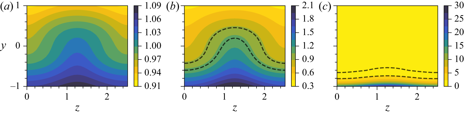


 Open access

