


1. Introduction
The collapse of a bubble near a material surface features a rapid, non-spherical compression of the internal gas, which may release mechanical and thermal energy in the forms of shock wave, liquid jet and increased local temperature. This process is a fundamental event in many science and engineering applications that involve cavitation, either as a harmful byproduct leading to erosion, noise and performance degradation, or as a useful mechanism for desired material modification and fabrication. Within the latter category, it has been demonstrated that the energy pulses released from bubble collapse may be used to remove contaminants or unwanted particles on a surface (Brems et al. Reference Brems, Hauptmann, Camerotto, Pacco, Kim, Xu, Wostyn, Mertens and De Gendt2014; Guo et al. Reference Guo, Khoo, Teo, Zhong, Lim and Lee2014), fabricate nanostructured solid materials (Xu, Zeiger & Suslick Reference Xu, Zeiger and Suslick2013), break agglomerates in a liquid metal (Kudryashova & Vorozhtsov Reference Kudryashova and Vorozhtsov2016), facilitate kidney stone destruction in shock wave lithotripsy (Zhong Reference Zhong2013), increase the permeability of human tissue or cell membrane for targeted drug/gene delivery (Coussios & Roy Reference Coussios and Roy2008; Brennen Reference Brennen2015) and mediate cellular mechanotransduction (Li et al. Reference Li, Yang, Yuan, Liao, Li, Guilak and Zhong2018) – just to name a few examples. A common issue in these applications is that the location, extent and intensity of cavitation need to be controlled carefully, as the boundary between meritorious effects and deleterious effects can be narrow. For example, using cavitation to remove biofouling on ship hulls needs to avoid damage to hull coatings (Guo et al. Reference Guo, Khoo, Teo, Zhong, Lim and Lee2014). In lithotripsy, cavitation bubbles can contribute to stone fragmentation; yet they may also damage human tissue and scatter the focused ultrasound waves (Zhong, Zhou & Zhu Reference Zhong, Zhou and Zhu2001; Pishchalnikov et al. Reference Pishchalnikov, Sapozhnikov, Bailey, Williams, Cleveland, Colonius, Crum, Evan and McAteer2003; Maeda et al. Reference Maeda, Maxwell, Colonius, Kreider and Bailey2018). Similarly, the use of cavitation to produce cell sonoporation produces therapeutic effects only when the detrimental side effects due to overdose do not occur (Ohl et al. Reference Ohl, Arora, Ikink, De Jong, Versluis, Delius and Lohse2006). In general, the need for controlled cavitation bubble collapse near various solid and soft materials calls for improved understanding of the two-way coupling between bubble dynamics and the material's response.
In the past, the non-spherical collapse of a bubble near different types of material boundaries has been studied using experimental and computational methods. The investigated material boundaries include a rigid wall (e.g. Zhang, Duncan & Chahine Reference Zhang, Duncan and Chahine1993; Brujan et al. Reference Brujan, Keen, Vogel and Blake2002; Calvisi, Iloreta & Szeri Reference Calvisi, Iloreta and Szeri2008; Johnsen & Colonius Reference Johnsen and Colonius2009; Brujan & Matsumoto Reference Brujan and Matsumoto2012; Wang Reference Wang2014), a surface of elastic solid bodies (e.g. Brujan et al. Reference Brujan, Nahen, Schmidt and Vogel2001; Sankin & Zhong Reference Sankin and Zhong2006), thin films (e.g. Turangan et al. Reference Turangan, Ong, Klaseboer and Khoo2006), a surface of soft tissues (e.g. Kodama & Takayama Reference Kodama and Takayama1998) and free liquid–gas interfaces (e.g. Blake & Gibson Reference Blake and Gibson1981; Robinson et al. Reference Robinson, Blake, Kodama, Shima and Tomita2001). The damage and fracture (e.g. pits, cracks, holes) in a nearby material after multiple cycles of bubble collapse have also been investigated (e.g. Philipp & Lauterborn Reference Philipp and Lauterborn1998; Dular, Delgosha & Petkovšek Reference Dular, Delgosha and Petkovšek2013). Nonetheless, knowledge of the dynamic response of different types of materials to bubble collapse – such as the amplitude, profile and propagation of surface and bulk elastic waves – is still limited. In this regard, a few teams (e.g. Freund, Shukla & Evan Reference Freund, Shukla and Evan2009; Kobayashi, Kodama & Takahira Reference Kobayashi, Kodama and Takahira2011) have applied Eulerian multiphase fluid dynamics solvers to simulate the interaction of collapsing bubbles with soft materials (e.g. biological tissues), in which the materials are modelled as fluids. Turangan et al. (Reference Turangan, Ball, Jamaluddin and Leighton2017) have applied a Lagrangian solver to simulate shock-induced bubble collapse near aluminium walls and foils. Chahine & Hsiao (Reference Chahine and Hsiao2015) have applied a fluid–solid coupled solver to simulate bubble collapse near metals and polymers, including the resulting permanent deformation (e.g. pitting). Wang (Reference Wang2017) has applied a fluid–solid coupled solver to simulate shock-bubble–stone interaction in the context of shock wave lithotripsy. Moreover, although a few studies using high-speed photography and acoustic measurements have revealed significant impact of the Young's modulus of the material on bubble dynamics (e.g. Gibson & Blake Reference Gibson and Blake1982; Brujan et al. Reference Brujan, Nahen, Schmidt and Vogel2001; Sankin & Zhong Reference Sankin and Zhong2006), the detailed reciprocal effects of the acoustic, elastic and viscoelastic properties of the material on bubble dynamics are still largely unknown.
In this paper, we present a computational study of shock-induced bubble collapse near different solid materials, focusing on describing the two-way fluid–material interaction and investigating the effect of the material's acoustic impedance. Specifically, we consider an air bubble in water next to a planar material boundary. We send an ultrasound shock wave with a sharp compressive front towards the bubble, which drives it to collapse. This setting is relevant to a number of ultrasound applications, and is possible to replicate in a laboratory environment. The acoustic impedance of a material is defined as  $Z=\rho c$, where
 $\rho$ and
 $c$ denote mass density and acoustic (
 $P$-wave) velocity, respectively. Our interest in the effect of
 $Z$ is motivated by two considerations. First, it is a fundamental material property that can often clearly distinguish different ‘hard’ and ‘soft’ materials in an application. Second, a few previous studies on bubble collapse near a rigid wall have indicated that the reflection of the shock wave against a material surface may have significant effects. For example, Calvisi et al. (Reference Calvisi, Iloreta and Szeri2008) highlighted that the reflected shock against a rigid wall intensifies the non-spherical bubble collapse. The results of Johnsen & Colonius (Reference Johnsen and Colonius2009) and Wang (Reference Wang2017) also support this finding. Acoustic impedance is a key parameter in wave reflection and transmission; a rigid wall can be considered as an extreme case with
 $Z=\infty$. Therefore, the finding mentioned above naturally suggests that it is valuable to investigate real materials with different (and finite) values of
 $Z$, including cases where its value is smaller than the acoustic impedance of the ambient fluid.
We employ a recently developed three-dimensional (3-D), multiphase fluid–solid coupled computational framework in this study (Wang, Lea & Farhat Reference Wang, Lea and Farhat2015; Huang, De Santis & Farhat Reference Huang, De Santis and Farhat2018). The important components of this framework relevant to the present study include: (a) an Eulerian finite volume, multiphase compressible Navier–Stokes equation solver, equipped with a level-set method for tracking the surface of the bubble; (b) a Lagrangian finite element solid mechanics (elasticity and viscoelasticity) solver; (c) an embedded boundary method for tracking the fluid–solid interface in an unstructured, non-interface-conforming fluid mesh (Wang et al. Reference Wang, Grétarsson, Main and Farhat2012; Huang et al. Reference Huang, De Santis and Farhat2018); (d) the FIVER (‘Finite Volume method with Exact multi-material Riemann solvers’) method for enforcing the interface conditions at the liquid–gas and fluid–solid interfaces (Wang et al. Reference Wang, Rallu, Gerbeau and Farhat2011; Farhat, Gerbeau & Rallu Reference Farhat, Gerbeau and Rallu2012; Main et al. Reference Main, Zeng, Avery and Farhat2017); and (e) a second-order, numerically stable partitioned procedure for coupling the fluid and solid solvers (Farhat et al. Reference Farhat, Rallu, Wang and Belytschko2010). This computational framework has been applied to simulate several fluid–structure interaction problems involving shock waves, large structural deformation, instability and fracture (e.g. Farhat et al. Reference Farhat, Wang, Main, Kyriakides, Lee, Ravi-Chandar and Belytschko2013; Wang et al. Reference Wang, Lea, Main, McGarity and Farhat2014; Chung et al. Reference Chung, Cao, Philen, Beran and Wang2018; Cao et al. Reference Cao, Zhang, Liao, Zhong and Wang2019). It has also been verified and validated for a few two-phase flow problems involving a bubble collapsing near a rigid wall (e.g. Farhat, Rallu & Shankaran Reference Farhat, Rallu and Shankaran2008; Main et al. Reference Main, Zeng, Avery and Farhat2017; Wang Reference Wang2017). For example, Main et al. (Reference Main, Zeng, Avery and Farhat2017) simulated a laboratory experiment of underwater bubble implosion, in which the gas content (air) is initially enclosed by a thin-walled glass sphere (Turner Reference Turner2007). They showed that the simulated pressure time history agrees favourably with the measurement obtained in the laboratory. In this work, we simulate the collapse of a bubble near a broad range of materials including metals (e.g. aluminium), polymers (e.g. polyurea), minerals (e.g. gypsum), glass and foams. In each case, we characterize the two-way fluid–material interaction using fluid pressure, velocity, bubble volume and the maximum tensile and shear stresses in the material. To highlight the effect of acoustic impedance on the dynamics of bubble collapse, we compare the bubble's collapse time, the minimum bubble volume, the jet velocity and the pressure load induced by the emitted shock wave on the material surface.
The remainder of this paper is organized as follows. Section 2 presents the physical model and numerical methods used in this study. Section 3.1 presents a verification of the computational framework using a 3-D benchmark problem featuring wave transmission and deflection at a fluid–solid interface. Section 4 presents the results of shock-induced bubble collapse near three representative materials, focusing on describing the two-way interaction between the fluid dynamics and the response of the material. Furthermore, § 5 presents a parametric study that considers different materials with acoustic impedance ranging from  $0.063$ to
 $17.28$ MPa
 $\cdot$s m
 $^{-1}$. We show that the effect of acoustic impedance on the bubble's collapse time and minimum volume can be captured using phenomenological models constructed based on the solution of the Rayleigh–Plesset equation. Finally, we provide a few concluding remarks in § 6.
2. Physical model and numerical methods
2.1. Governing equations and constitutive models
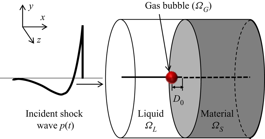
We consider a 3-D spatial domain comprised of multiple subdomains occupied by different fluid and solid materials. Figure 1 presents a schematic drawing of the problem set-up. A spherical gas bubble with a radius of  $R_{0}$ is placed in a liquid at a standoff distance
 $D_{0}$ from the solid material (measured from the centre of the bubble). An incident shock wave propagates towards the bubble from the opposite side, causing its collapse. Let
 $\varOmega _{G}$,
 $\varOmega _{L}$ and
 $\varOmega _{S}$ denote the subdomains occupied by the bubble, the ambient fluid (liquid) and the solid material, respectively. We model both the gas inside the bubble and the ambient fluid as compressible inviscid fluids. Dropping of viscosity can be justified by the high pressure of the incident shock wave in the current problem set-up (see, e.g. Brujan (Reference Brujan2019) for a different and more complex fluid environment) and a relatively small time frame considered within this study.
A 3-D fluid–solid coupled model of shock-induced bubble collapse near a solid or soft material.

Therefore, in  $\varOmega _{G}$ and
 $\varOmega _{L}$, we solve the following Euler equations in the Eulerian frame:
 \begin{equation} \frac{\partial \boldsymbol{W}(\boldsymbol{x},t)}{\partial t} + \boldsymbol{\nabla} \boldsymbol{\cdot} \mathcal{F}(\boldsymbol{W}) = 0, \quad \forall \, \boldsymbol{x} \in \varOmega_{L}(t) \cup \varOmega_{G}(t), \ t>0,\end{equation}
with
 \begin{equation} \boldsymbol{W}=\begin{bmatrix} \rho \\ \rho \boldsymbol{V} \\ \rho e_{t} \end{bmatrix}, \quad \mathcal{F} = \begin{bmatrix} \rho \boldsymbol{V}^T \\ \rho \boldsymbol{V} \otimes \boldsymbol{V} + p \boldsymbol{\boldsymbol{\mathsf{I}}} \\ (\rho e_{t} + p)\boldsymbol{V}^T \end{bmatrix}, \end{equation}
where  $\rho$,
 $\boldsymbol{V}$,
 $p$ and
 $e_{t}$ denote the fluid density, velocity, pressure and the total energy per unit mass, respectively;
 $\boldsymbol{\boldsymbol{\mathsf{I}}}$ is the
 $3\times 3$ identity matrix. Equation (2.1) is closed by an equation of state (EOS) for each fluid material. We apply the perfect gas EOS to the gas inside the bubble, i.e.
 \begin{equation} p=( \gamma_{G} -1 ) \rho e ,\end{equation}
where  $\gamma _{G}$ is the heat capacity ratio, and
 $e$ is the internal energy per unit mass. In this work, we set
 $\gamma _{G}=1.4$. We assume the ambient fluid is water, and apply the stiffened equation of state, i.e.
 \begin{equation} p = ( \gamma_{L}-1 ) \rho e - \gamma_{L} p_{L},\end{equation}
where  $\gamma _{L}=6.59$ and
 $p_{L}=410$ MPa (Johnsen & Colonius Reference Johnsen and Colonius2008).
Within the subdomain of the solid material, i.e.  $\varOmega _S$, we adopt the Lagrangian frame and solve the following equation of motion that enforces the balance of linear momentum:
 \begin{equation} \rho_{s} \ddot{\boldsymbol{u}}(\boldsymbol{X},t) - \boldsymbol{\nabla} \boldsymbol{\cdot} \boldsymbol{\sigma} (\boldsymbol{u},\dot{\boldsymbol{u}}) = \boldsymbol{b}, \quad \forall \, \boldsymbol{X} \in \varOmega_{S}(0), \ t >0, \end{equation}
where  $\boldsymbol {u}$ denotes displacement,
 $\rho _{s}$ the material's mass density and
 $\boldsymbol {\sigma }$ the Cauchy stress tensor;
 $\boldsymbol {b}$ denotes the body force acting in
 $\varOmega _{S}$, which is assumed to be zero in this study.
We adopt the generalized Maxwell model of viscoelasticity (Cheneler Reference Cheneler2016), which combines linear springs and linear dashpots. Assuming zero strain at  $t=0$, the stress at any time instance
 $t>0$ can be written in the form of the hereditary integral,
 \begin{equation} \boldsymbol{\sigma}(t) = \int^{t}_{0} G_{R}(t-s) \frac{\textrm{d} \boldsymbol{\epsilon}(s)}{\textrm{d} s}\ \textrm{d} s, \end{equation}
where  $\boldsymbol{\epsilon}$ denotes the strain tensor;
 $G_{R}(t)$ is the relaxation modulus. In this work, we express
 $G_{R}(t)$ as a Prony series, i.e.
 \begin{equation} G_{R}(t) = G_{0} \left[ 1 - \sum^{N}_{i=1} g_{i} ( 1 - \textrm{e}^{-t/\tau_{i}} ) \right], \end{equation}
where  $G_{0}=G_{R}(0)$ is the instantaneous modulus,
 $g_{i}$ and
 $\tau _{i}$ are material-specific model parameters. The Prony series is appealing particularly from a numerical viewpoint, as it does not require storing of the time history of strain. Specifically, we compute
 $\sigma (t)$ using a recursive formula, as shown in Goh, Charalambides & Williams (Reference Goh, Charalambides and Williams2004).
For some of the materials investigated in this study (e.g. a strengthened gypsum, metals), the viscoelastic effect of the material is negligible. These materials are modelled essentially by linear elasticity, with constitutive equation
 \begin{equation} \boldsymbol{\sigma} = \frac{E\nu}{(1+\nu)(1-2\nu)} tr(\boldsymbol{\boldsymbol{\epsilon}})\boldsymbol{\boldsymbol{\mathsf{I}}} + \frac{E}{1+\nu} \boldsymbol{\epsilon}, \end{equation}
where  $E$ and
 $\nu$ are the Young's modulus and Poisson's ratio of the material, respectively;
 $tr(\cdot )$ denotes the trace operator.
At the fluid–solid interface,  $\varGamma _{FS} = \partial \varOmega _{S}(t) \cap (\partial \varOmega _{L}(t) \cup \partial \varOmega _{G}(t))$, we enforce the continuity of normal velocity and surface traction, i.e.
 \begin{equation} \left. \begin{array}{l} (\boldsymbol{V} - \dot{\boldsymbol{u}})\boldsymbol{\cdot} \boldsymbol{n} = 0, \\ -p\boldsymbol{n} = \boldsymbol{\sigma}(\boldsymbol{u},\dot{\boldsymbol{u}})\boldsymbol{\cdot} \boldsymbol{n}, \end{array}\right. \quad \hbox{on } \varGamma_{FS},\end{equation}
where  $\boldsymbol {n}$ denotes the unit normal to
 $\varGamma _{FS}$.
At the liquid–gas interface,  $\varGamma _{FF}(t) = \partial \varOmega _{L}(t) \cap \partial \varOmega _{G}(t)$, we assume that the two fluid materials are immiscible. Also, surface tension is negligible compared to the pressure of the prescribed shock wave. Thus, the interface conditions are those describing a contact discontinuity, i.e.
 \begin{equation} \left. \begin{array}{l} (\boldsymbol{V}_{L}-\boldsymbol{V}_{G}) \boldsymbol{\cdot} \boldsymbol{n} = 0, \\ p_{L} = p_{G}, \end{array} \right. \quad \hbox{on }\varGamma_{FF}.\end{equation}
2.2. Fluid–solid coupled computational framework
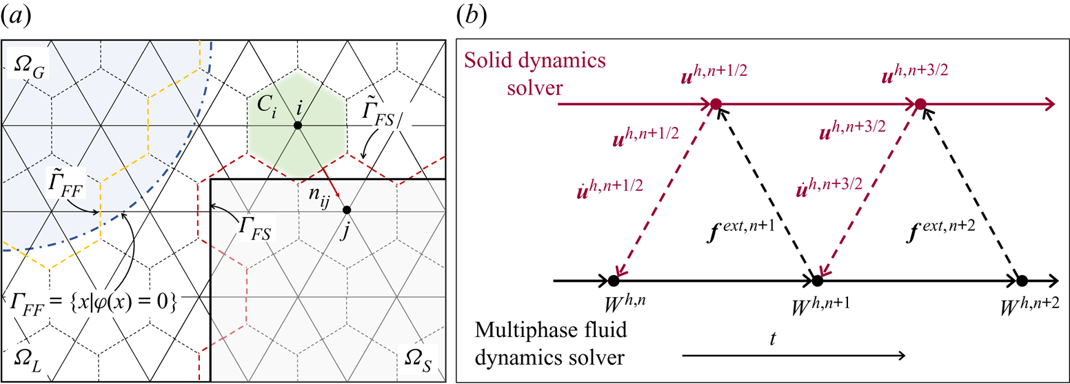
We apply a recently developed fluid–solid coupled computational framework to solve the above model equations. The framework couples a finite volume, multiphase compressible flow solver with a finite element solid dynamics solver using an embedded boundary method and a staggered partitioned procedure (figure 2).
Illustration of the spatial (a) and temporal (b) discretization methods applied in the computational framework.

As illustrated in figure 2(a), the fluid governing equations are semi-discretized in an augmented fluid domain,  $\tilde {\varOmega } = \varOmega _L \cup \varOmega _G \cup \varOmega _S$, using an unstructured, node centred, non-interface-conforming finite volume mesh, denoted by
 $\tilde {\varOmega }^{h}$. For each node of the mesh (e.g. node
 $i$), a dual cell (i.e. control volume)
 $C_{i}$ is constructed. Integrating (2.1) within
 $C_i$ gives
 \begin{equation} \frac{\partial \boldsymbol{W}_i}{\partial t} + \frac{1}{\lVert C_i \rVert} \sum_{j\in Nei(i)} \int_{\partial C_{ij}} \mathcal{F}(\boldsymbol{W})\boldsymbol{\cdot} \boldsymbol{n}_{ij} \ \textrm{d} S = 0, \end{equation}
where  $\boldsymbol{W}_i$ denotes the average of
 $\boldsymbol{W}$ in
 $C_i$,
 $\lVert C_i \rVert$ denotes the volume of
 $C_i$,
 $Nei(i)$ denotes the set of nodes connected to node
 $i$ by an edge,
 $\partial C_{ij} = \partial C_i \cap \partial C_j$ and
 $\boldsymbol {n}_{ij}$ is the unit normal to
 $\partial C_{ij}$. Depending on the location of nodes
 $i$ and
 $j$, four scenarios arise in the calculation of the surface integral over
 $\partial C_{ij}$:
(a) If nodes
 $i$ and $j$ belong to the same fluid subdomain ($\varOmega _L$ or $\varOmega _G$), the flux across $\partial C_{ij}$ is calculated using the well-known monotonic upwind scheme conservation law (MUSCL) scheme (Van Leer Reference Van Leer1979) and Roe's flux (Roe Reference Roe1981).
(b) If nodes
$i$ and $j$ belong to different fluid subdomains (i.e. one in $\varOmega _L$, the other in $\varOmega _G$), a one-dimensional (1-D) two-fluid Riemann problem is constructed along edge $i$–$j$, i.e.
(2.12)where\begin{equation} \frac{\partial \boldsymbol{w}}{\partial \tau} + \frac{\partial \mathcal{F}(\boldsymbol{w})}{\partial \xi} = 0, \quad \text{with } \boldsymbol{w}(\xi,0)=\begin{cases} \boldsymbol{w}_{i} & \text{if } \xi \leq 0,\\ \boldsymbol{w}_{j} & \text{if } \xi > 0, \end{cases} \end{equation}$\tau$ denotes the time coordinate; $\xi$ denotes the spatial coordinate along the 1-D axis aligned with $\boldsymbol {n}_{ij}$ and centred at the midpoint between nodes $i$ and $j$. The initial states $\boldsymbol {w}_{i}$ and $\boldsymbol {w}_{j}$ are projections of $\boldsymbol{W}_{i}$ and $\boldsymbol{W}_{j}$ on the $\xi$ axis. Equations (2.10) are enforced at the moving interface for $\tau >0$. The exact solution of this 1-D Riemann problem is supplied to Roe's flux function to compute the flux across $\partial C_{ij}$ (Farhat et al. Reference Farhat, Gerbeau and Rallu2012).(c) If one of the two nodes (e.g. node
$i$) belongs to a fluid subdomain ($\varOmega _L$ or $\varOmega _G$), while the other node belongs to the solid subdomain ($\varOmega _S$), a 1-D fluid–solid Riemann problem with a moving wall boundary is constructed, i.e.
(2.13)\begin{gather} \frac{\partial {\boldsymbol{w}}}{\partial \tau} + \frac{\partial {\mathcal{F}}({\boldsymbol{w}})}{\partial \xi} = 0, \quad \tau>0,\ \xi < v_S \tau, \end{gather}(2.14)\begin{gather}{\boldsymbol{w}}(\xi,0) = \boldsymbol{w}_i, \quad \xi<0, \end{gather}(2.15)where\begin{gather}v(v_S\tau,\tau) = v_S, \quad \tau>0, \end{gather}$\xi$ is the spatial coordinate along the normal direction of the fluid–solid interface and centred at the midpoint between nodes $i$ and $j$. The initial state $\boldsymbol {w}_i$ is the reconstructed fluid state at the interface; $v$ denotes the fluid velocity at the moving wall boundary, and $v_S$ the normal velocity of the wetted surface of the solid structure (i.e. the fluid–solid interface) at its intersection with fluid edge $i$–$j$, which is computed by the solid dynamics solver. Similar to the previous case, the exact solution of this 1-D Riemann problem is supplied to Roe's flux function to compute the flux across $\partial C_{ij}$ (Wang et al. Reference Wang, Rallu, Gerbeau and Farhat2011).(d) If nodes
$i$ and $j$ both belong to the solid subdomain ($\varOmega _S$), the flux across $\partial C_{ij}$ is set to $0$.


The above method is referred to as FIVER (Farhat et al. Reference Farhat, Gerbeau and Rallu2012). It is ideally suited for solving the present problem, as the problem involves both multi-fluid (i.e. liquid–gas) and fluid–solid interfaces.
FIVER requires tracking of the liquid–gas and fluid–solid interfaces in the unstructured, non-interface-conforming mesh  $\tilde {\varOmega }^{h}$. We track the evolution of the liquid–gas interface by solving the level-set equation,
 \begin{equation} \frac{\partial \phi(\boldsymbol{x},t)}{\partial t} + \boldsymbol{V} \boldsymbol{\cdot} \boldsymbol{\nabla} \phi = 0, \quad \forall \, \boldsymbol{x}\in \varOmega_L \cup \varOmega_G \cup \varOmega_S, \end{equation}
where  $\phi (\boldsymbol {x},t)$ represents the signed shortest distance from
 $\boldsymbol {x}$ to the interface. In this way, the large deformation and topological changes (e.g. splitting and merging) of the bubble surface are naturally accommodated. To track the fluid–solid interface, we apply a collision-based computational geometry algorithm as presented in Wang et al. (Reference Wang, Grétarsson, Main and Farhat2012, Reference Wang, Lea and Farhat2015).
In this work, (2.16) is recast in the form
 \begin{equation} \frac{\partial \phi}{\partial t} + \boldsymbol{\nabla} \boldsymbol{\cdot} (\phi \boldsymbol{V}) = \phi\boldsymbol{\nabla} \boldsymbol{\cdot} \boldsymbol{V}, \end{equation}
and solved on the same fluid mesh using a finite volume method. The convection term,  $\boldsymbol {\nabla } \boldsymbol {\cdot } (\phi \boldsymbol{V})$, is discretized using the MUSCL scheme with the upwinding flux. The term
 $\phi \boldsymbol {\nabla } \boldsymbol {\cdot} \boldsymbol{V}$ is added as a source term. Additional numerical details can be found in Main et al. (Reference Main, Zeng, Avery and Farhat2017) and Main (Reference Main2014).
A standard Galerkin finite element method is used to semi-discretize the weak form of (2.5), which yields
 \begin{equation} {\boldsymbol{\mathsf{M}}}\frac{\partial^2 \boldsymbol{u}^h}{\partial t^2} + \boldsymbol{f}^{int}\left(\boldsymbol{u}^h, \frac{\partial\boldsymbol{u}^h}{\partial t}\right) = \boldsymbol{f}^{ext},\end{equation}
where  ${\boldsymbol{\mathsf{M}}}$ denotes the mass matrix,
 $\boldsymbol {u}^h$ denotes the discrete displacement vector;
 $\boldsymbol {f}^{int}$ and
 $\boldsymbol {f}^{ext}$ denote the discrete internal force and external force vector, respectively.
We use a staggered fluid–solid time integrator presented in Farhat et al. (Reference Farhat, Rallu, Wang and Belytschko2010) to advance the fluid and solid subsystems. The fluid subsystem is time integrated using the explicit fourth-order Runge–Kutta scheme, while the solid subsystem is time integrated using the second-order central difference scheme. Notably, the fluid and solid time steps are offset by half a step (figure 2b). This is a designed feature to achieve second-order accuracy in time while maintaining optimal numerical stability.
3. Verification and validation of the computational framework
3.1. Wave propagation across a plane fluid–solid interface
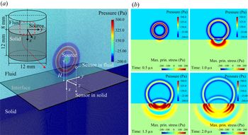
We first apply the computational framework described in § 2.2 to solve a 3-D model problem featuring the propagation of an impulsive pressure wave across a planar fluid–solid interface. The objective is to verify the computational framework for predicting wave transmission and deflection at a fluid–solid interface, which is an important feature of the bubble–material interaction problem under investigation. Figure 3(a) presents the set-up of the problem. We consider a cylindrical fluid–solid domain with a diameter of  $12$ mm and a height of
 $20$ mm. In the fluid subdomain, we impose a spherical pressure wave generated from a monopole source, similar to the shock wave emitted from the rapid collapse of a bubble. Specifically, we specify a Ricker wavelet, which is widely used as a model of the seismic waves from a point excitation. Table 1 shows the geometric and material information involved in the simulation.
(a) Problem set-up (the dynamic pressure of the fluid at  $t = 0$ is visualized). (b) Snapshots of numerical solution at four different time instances, showing the dynamic pressure of the fluid and the maximum principal stress in the solid.

Parameters of the verification problem.

 $c_{L}$: longitudinal wave speed;
 $c_{T}$: transverse wave speed.
We prescribe the Ricker wavelet as the initial condition of the fluid. Specifically, the initial pressure at a distance  $r$ from the source is given by
 \begin{equation} p(r) = p_{0} + \frac{Q(-r/c_{0})}{r}, \end{equation}
with
 \begin{equation} Q(s) = [ 1-2{\rm \pi}^{2}f_{0}^{2}(s+s_{1})^2 ] \exp({-{\rm \pi}^2f_{0}^2 (s+s_{1})^2}), \end{equation}
where  $p_{0}$ denotes the hydrostatic pressure,
 $c_{0}$ the speed of sound in the fluid,
 $f_{0}$ the frequency of Ricker wavelet and
 $s_{1}$ is a constant that controls the initial position of the wavelet. The values of these parameters are given in table 1. The initial velocity of the fluid is then prescribed according to the acoustic theory. The initial pressure wave has a peak magnitude of
 $913$ Pa and a width of
 ${\sim }2$ mm in the radial directions (figure 3a). Its central peak is located at
 ${\sim }1.31$ mm above the material surface.
The simulation is carried out using an unstructured, finite volume fluid mesh with  $21.9$ million tetrahedral elements and a finite element solid mesh with
 $6.7$ million tetrahedral elements. In the most refined region, the characteristic element size is approximately
 $0.01$ mm for the fluid and
 $0.04$ mm for the solid. A constant time step size of
 $5.0 \times 10^{-4}\ \mathrm {\mu }$s is used in both solvers.
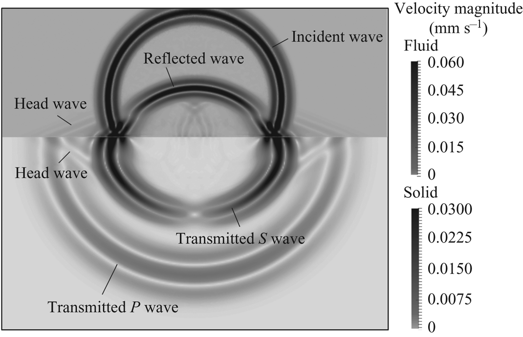
Figure 3(b) presents the numerical solution at four time instances, showing the fluid pressure field and the maximum principal stress in the solid. The simulation captures the transient dynamics of wave propagation across the fluid–solid interface, including the reflection of the pressure wave and the elastodynamic response of the solid. More specifically, figure 4 shows different types of waves that occur at a specific time instance, including the incident and the reflected waves in the fluid, the longitudinal (or  $P$) and transverse (or
 $S$) waves in the solid, and the head waves generated by the advancing of the transmitted
 $P$ wave along the interface.
Velocity field at  $t = 3\ \mathrm {\mu }$s. The incident and reflected waves in the fluid, the transmitted waves in the solid and the head wave generated at the interface are clearly captured.

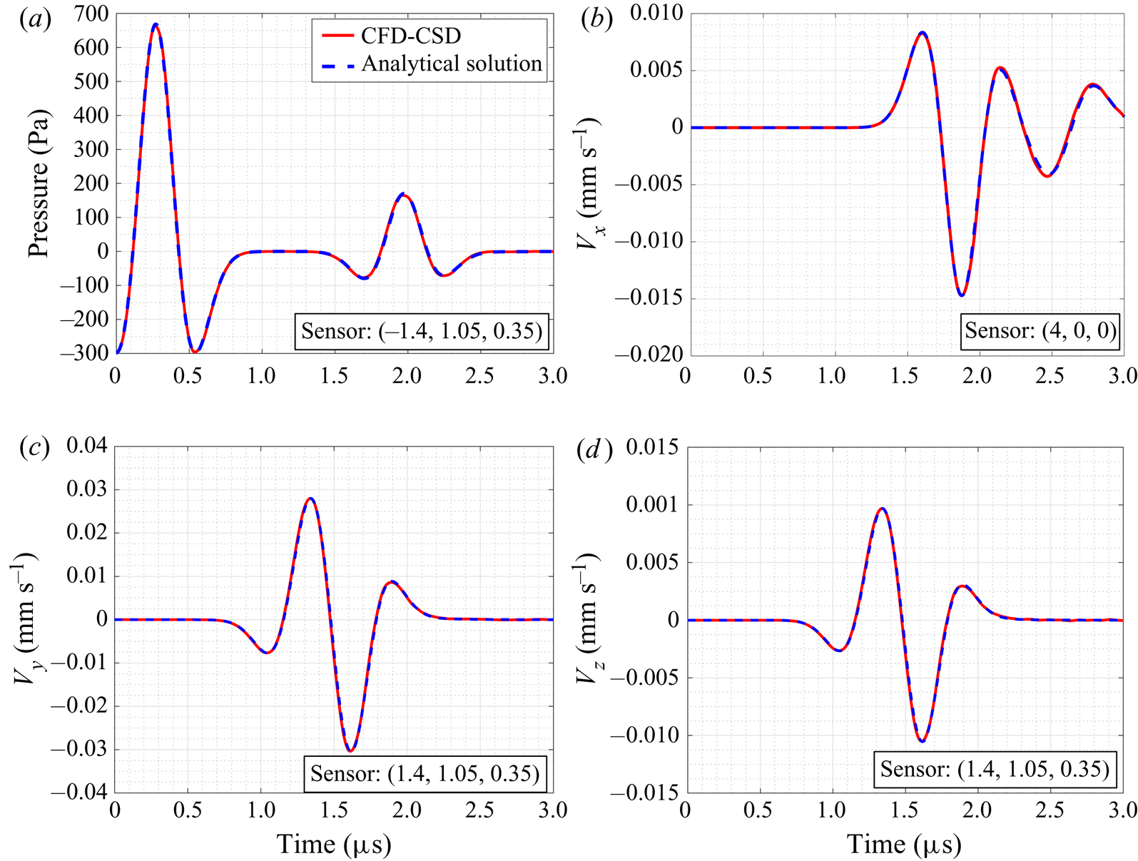
In this problem, the maximum dynamic pressure in the fluid is two orders of magnitude smaller than the hydrostatic pressure. Therefore, the incident wave can be considered as a small disturbance and modelled as an acoustic wave propagating in a homogeneous fluid medium. Given the assumption that the solid material is isotropic and linear elastic, this problem can thus be modelled adequately by coupling the linear acoustic wave equation with the equation of motion for a linear elastic solid. The exact solution of this problem can be obtained using the Cagniard–de Hoop method (de Hoop & Van der Hijden Reference de Hoop and Van der Hijden1984), therefore providing a reliable reference for verifying our numerical solver. We use an open-source code, Gar6more3D (INRIA 2013), to compute the exact solution. Figure 5 presents a comparison of the numerical and the analytical solutions at three sensors located in the fluid and in the solid. A close agreement is obtained. For example, the peak dynamic pressure recorded at sensor ( $-$1.4, 1.05, 0.35) mm differs by only
 $0.66\,\%$ between the numerical and the analytical solutions.
Comparison of the numerical solution obtained using the CFD (computational fluid dynamics) – CSD (computational solid dynamics) coupled solver with the analytical solution. (a) Time history of pressure at sensor ( $-$1.4, 1.05, 0.35) mm in the fluid. (b–d) Time history of velocity at sensors (4, 0, 0) mm and (1.4, 1.05, 0.35) mm in the solid.

3.2. Collapse of a spherical bubble in an infinite medium
To demonstrate the numerical model's capability of capturing single bubble dynamics, we simulate the collapse of a spherical bubble in an infinite liquid medium. The simulation is based on the experiment of Kröninger et al. (Reference Kröninger, Köhler, Kurz and Lauterborn2010) in which the dynamics of a laser-generated spherical bubble in water is captured using high-speed photography. We focus on simulating the initial collapse of the bubble from its maximum radius  $R_{0}=0.747$ mm. We assume that when the bubble is at its maximum size, velocity is zero both inside and outside of the bubble, and the thermodynamic variables have constant values within each subdomain. Specifically, the initial density and pressure of liquid water are set to
 $1000$ kg m
 $^{-3}$ and
 $0.101$ MPa, respectively; and the stiffened equation of state described in § 2.1 is applied. The composition and state of the gas inside the bubble was not measured in the experiment. In the simulation, we set the gas material to be air, modelled using the perfect gas equation of state ((2.3)). In previous computational studies, the initial state of the bubble is often estimated via theoretical models or data fitting (e.g. Müller et al. Reference Müller, Bachmann, Kröninger, Kurz and Helluy2009; Koch et al. Reference Koch, Lechner, Reuter, Köhler, Mettin and Lauterborn2016) due to the lack of experimental data. Although the time history of bubble radius in those studies shows good agreement with the experimental data, the initial pressure and temperature applied therein are often unrealistically small (e.g.
 $p_{0} = 4.579\ \text {Pa}$ in Müller et al. Reference Müller, Bachmann, Kröninger, Kurz and Helluy2009). Here, we apply the initial density calculated in Müller et al. (Reference Müller, Bachmann, Kröninger, Kurz and Helluy2009) (i.e.
 $\rho _{0}=0.957\times 10^{-3}$ kg m
 $^{-3}$) but use a more realistic initial pressure,
 $p_{0} = 100$ Pa. Leveraging the spherical symmetry in this problem, the computational domain is set to be a tall and slender tetrahedron whose apex coincides with the centre of the bubble, with symmetric boundary condition applied at its three side surfaces.
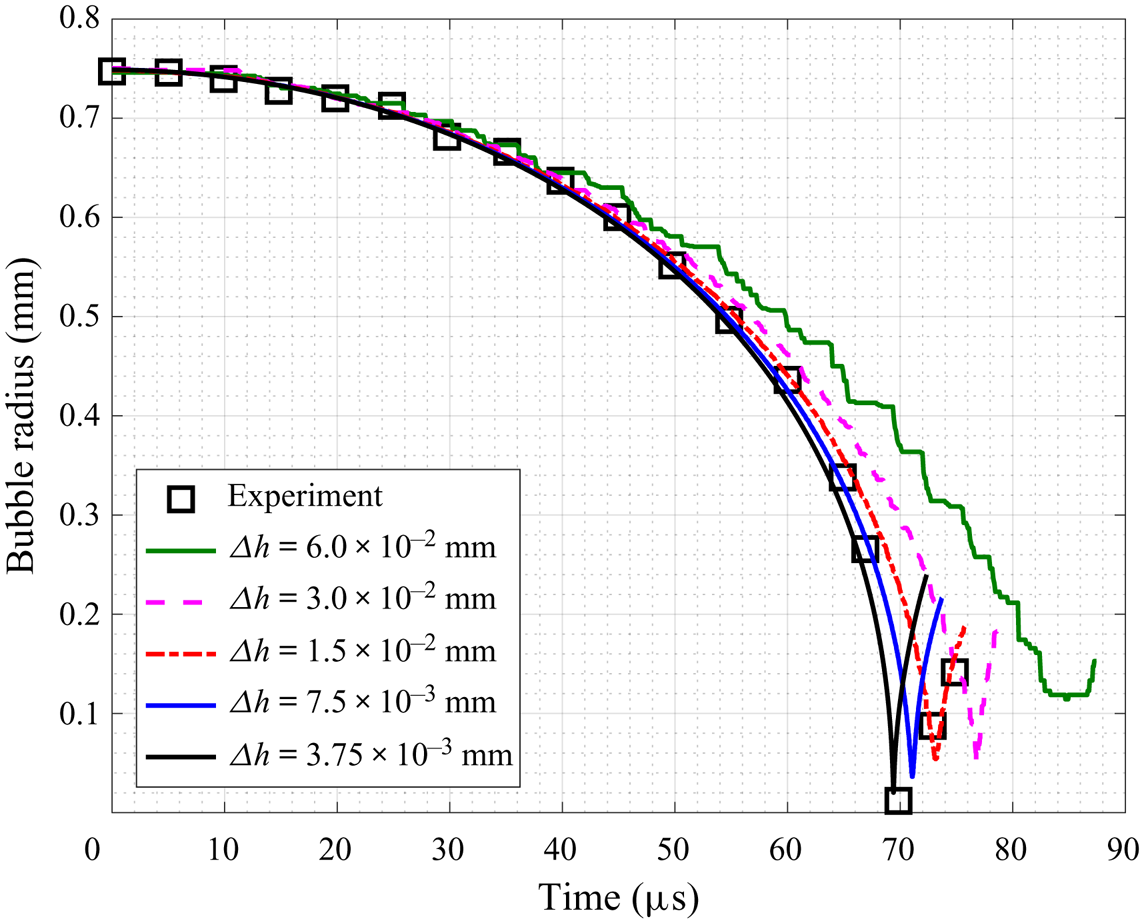
Five simulations are carried out using meshes of different resolutions. Specifically, the characteristic element size ( $\varDelta h$) within and around the region of the bubble is refined from
 $60$ to
 $3.75\ \mathrm {\mu }$m.
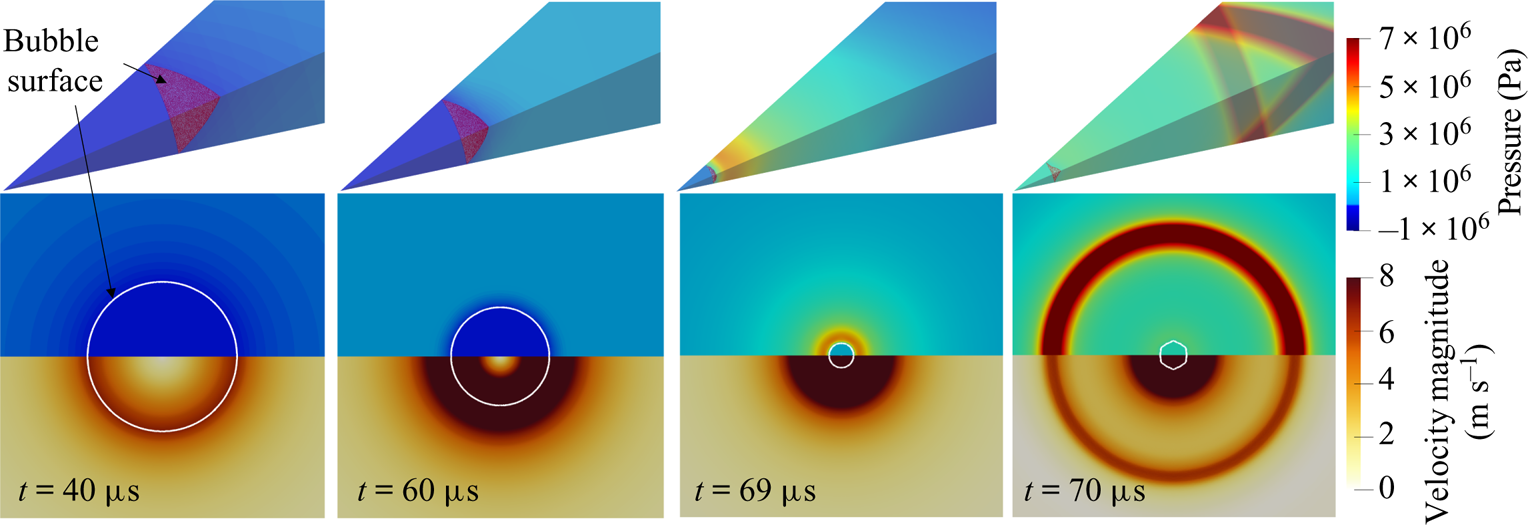
Figure 6 presents the time evolution of bubble radius obtained using the five meshes. Evidently, as the mesh gets refined, the numerical result converges gradually to the experimental data for the period of bubble collapse. Figure 7 presents the velocity magnitude and the pressure field around bubble at four time instances for the converged solution. Driven by pressure difference, the bubble interface accelerates toward its interior and remains spherical during the collapse. When the bubble reaches its minimum volume, a strong shock wave is emitted.
Comparison between numerical results and experimental data for the time history of bubble radius. Five sets of numerical result obtained with different mesh resolutions ( $\varDelta h$) are presented (the radius is calculated based on the volume of the gas domain). The experimental data are extracted from Kröninger et al. (Reference Kröninger, Köhler, Kurz and Lauterborn2010).

Converged solution at four time instances during collapse. Upper figure: pressure field in the tetrahedron computational domain. Lower figure: pressure and velocity magnitude in a 2-D plane across the bubble centre (the white curve represents the bubble surface). The full solution field is reconstructed by post-processing (reflection) the solution field on a plane across the apex of the tetrahedron domain.

It is noteworthy that for the time period of the bubble's rebound, the converged numerical result does not closely match the experimental data. This is likely due to the fact that the numerical model does not account for some physical processes (e.g. liquid/gas phase change) that become important when the bubble is at its minimum volume, as well as the inconsistent modelling of the bubble content (c.f. Koch et al. Reference Koch, Lechner, Reuter, Köhler, Mettin and Lauterborn2016). However, since the main focus of this work is the initial collapse of the bubble, the agreement with the experimental data presented above provides support for the validity of the numerical model.
4. Shock-induced bubble collapse near three representative materials
4.1. Set-up of numerical experiment
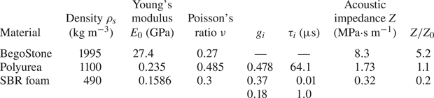
In this section, we consider shock-induced bubble collapse near three representative materials, namely a strengthened gypsum (BegoStone 15 : 3, Esch et al. Reference Esch, Simmons, Sankin, Cocks, Preminger and Zhong2010; Simmons et al. Reference Simmons, Cocks, Zhong and Preminger2010), an elastomer (polyurea P1000, Amirkhizi et al. Reference Amirkhizi, Isaacs, McGee and Nemat-Nasser2006; Chahine & Hsiao Reference Chahine and Hsiao2015) and a foam rubber (Rubatex R8702 styrene-butadiene rubber (SBR) foam, Deigan Reference Deigan2007). Table 2 summarizes the main properties of these materials. In particular, the relative acoustic impedance of the material compared to that of the ambient fluid (i.e.  $Z/Z_{0}$) varies from
 $5.2$ in the case of BegoStone to
 $1.1$ in the case of polyurea and
 $0.2$ in the case of the foam. Both polyurea and the SBR foam are modelled as a viscoelastic material. For the BegoStone, viscoelastic effects are negligible within the small time frame considered in this study, therefore it is modelled as a purely elastic material. As a reference, we also simulate the same bubble collapsing near a rigid wall, which can be considered as a material with infinite acoustic impedance.
Material properties of three representative materials.

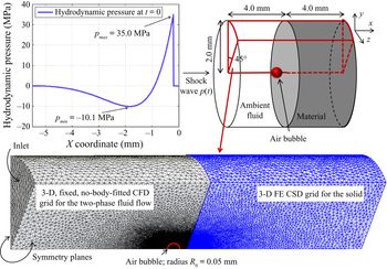
Figure 8 shows the set-up of the numerical experiment. Initially, a spherical air bubble with a radius of  $R_{0}=0.05$ mm is placed in the liquid, at a distance of
 $D_{0}=2R_{0}$ from the material surface (measured from the centre of the bubble). The incident shock wave that induces the bubble's collapse is adopted from Johnsen & Colonius (Reference Johnsen and Colonius2008). It has a compressive front with a positive peak of
 $35$ MPa, followed by a tensile phase with a negative peak of
 $10.1$ MPa (figure 8). This type of waveform can be generated in water through electrohydraulic or electromagnetic mechanisms (e.g. Church Reference Church1989; Fovargue et al. Reference Fovargue, Mitran, Smith, Sankin, Simmons and Zhong2013). We prescribe the incident shock wave as the initial condition of the fluid governing equations, following the method described in Cao et al. (Reference Cao, Zhang, Liao, Zhong and Wang2019). Away from the incident shock wave, the ambient flow velocity and hydrostatic pressure are set to
 $v_0 =0$ mm s
 $^{-1}$ and
 $p_{0}=0.101$ MPa, respectively. The 3-D model described in § 2.1 is applied. Notably, this problem can also be simulated using a 2-D axisymmetric model, which may be computationally less expensive. Nonetheless, the 3-D model can be easily extended in future to investigate more complicated cases without rotational symmetry, such as problems involving multi-bubble interaction and misalignment between the shock wave and the bubble. For computational efficiency, we consider a
 $45^{\circ }$ slice of the cylindrical domain with symmetry boundary conditions applied to the two cut planes, instead of modelling the entire 3-D domain. The computational domains for the solid and the fluid are discretized using
 $2.3$ million and
 $19.6$ million tetrahedron elements, respectively. The meshes are refined within a region close to the bubble and the fluid–solid interface, where the characteristic element size is
 $\varDelta h_{f} = 1.5\ \mathrm {\mu }\text {m}$ for the fluid mesh and
 $\varDelta h_{s} = 3\ \mathrm {\mu }\text {m}$ for the solid mesh. For comparison, the compressive front of the incident shock wave is approximately
 $700\ \mathrm {\mu }\text {m}$ in the liquid.
Set-up of numerical experiment. A shock wave with a magnitude of  $35$ MPa is applied to trigger the collapse of an air bubble with radius
 $R_{0}=0.05$ mm located at
 $D_{0}=2R_{0}$ from the material surface. Computations are performed on a
 $45^{\circ }$ slice of the cylindrical fluid–solid domain.

4.2. Result and discussion
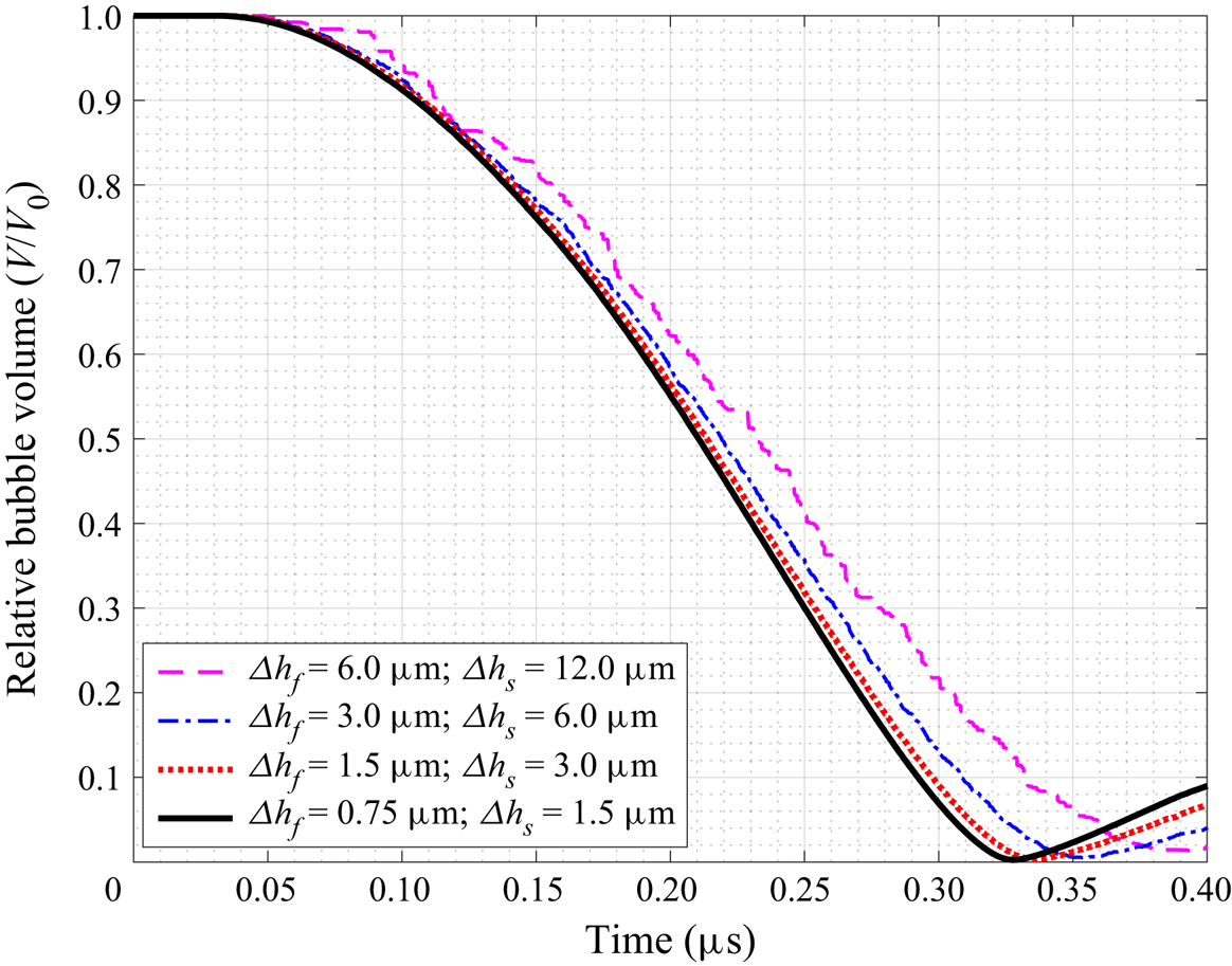
First, a mesh convergence analysis is performed for the case of BegoStone. Four sets of mesh, including the baseline mesh introduced in § 4.1, are tested. Within the region close to the bubble, the fluid element size ( $\varDelta h_{f}$) varies from
 $6.0$ to
 $0.75\ \mathrm {\mu }$m and the solid element size (
 $\varDelta h_{s}$) varies accordingly from
 $12.0$ to
 $1.5\ \mathrm {\mu }$m. Figure 9 presents the time history of relative bubble volume obtained with the four sets of mesh, showing the convergence of the results. The bubble's collapse time obtained with the finest mesh and the baseline mesh differ by less than
 $3\,\%$.
Mesh convergence analysis: time history of bubble volume obtained using four sets of mesh with refined characteristic element size ( $\varDelta h$) within the region close to the bubble.

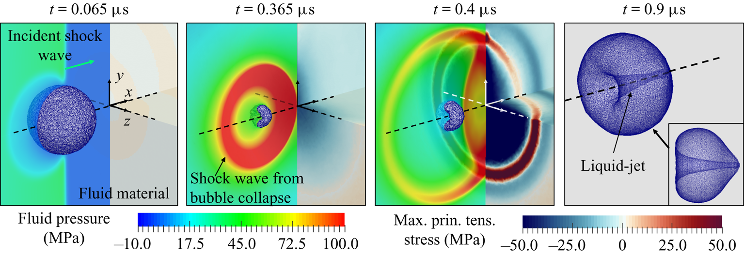
Figure 10 presents four solution snapshots from the case of BegoStone. Several key features are clearly captured. The impact of the incident shock wave at the proximal (left) side of the bubble triggers the bubble's collapse. When the bubble reaches its minimum volume, a shock wave is generated. Also, during the non-spherical bubble collapse, a liquid jet forms and penetrates the bubble. These features are consistent with the results of several previous studies that considered bubble collapse near a rigid wall (e.g. Johnsen & Colonius Reference Johnsen and Colonius2008; Kobayashi et al. Reference Kobayashi, Kodama and Takahira2011). A remarkable feature of the current result is that it captures the transmission and reflection of the shock waves at the fluid–solid interface, as well as the resulting elastic waves inside the material.
Shock-induced bubble collapse near BegoStone: transient fluid pressure, maximum principal stress inside the material and on its surface and the deformation of the bubble. The bubble's surface is captured by the  $0$ level set of the distance function
 $\phi (\boldsymbol {x},t)$.

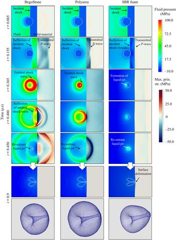
When the same bubble collapses near different materials, the dynamics of the bubble, the fluid flow, the pressure on the material surface and the stress inside the material all vary. Figure 11 provides a comparison of the three cases by showing the fluid pressure field and the maximum principal stress inside the solid at six time instances. The first major difference lies in the reflection of the incident shock wave at the material surface. This can be observed from the second row of images in figure 11, which are taken at  $t = 0.155\ \mathrm {\mu }\text {s}$, when the reflection has just reached the distal (right) side of the bubble. In the case of BegoStone, the reflected wave is compressive, with peak pressure around
 $23\ \text {MPa}$. In the case of polyurea, the reflected wave is also compressive, but its amplitude is only
 ${\sim }2\ \text {MPa}$. By contrast, the reflection is a tensile wave in the case of the foam, with peak pressure around
 $-25\ \text {MPa}$. At the same time, a fraction of the incident wave is transmitted into the material as a compressive stress wave. Figure 11 shows that both the amplitude and the propagation speed of the wave vary from case to case. The peak value of the maximum principal stress is found to be around
 $-57\ \text {MPa}$ (compressive) for BegoStone,
 $-35\ \text {MPa}$ for polyurea and
 $-10\ \text {MPa}$ for the foam.
Shock-induced bubble collapse near three different materials: fluid pressure and maximum principal stress.

The differences described above can be explained by the relative acoustic impedance of each material compared to that of the ambient fluid (i.e.  $Z/Z_0$). Consider a simplified one-dimensional problem in which an incident wave with amplitude
 $p_{i}$ impinges on a surface in its normal direction. According to the acoustic wave theory Brekhovskikh & Godin Reference Brekhovskikh and Godin2012), the amplitude of the reflected and transmitted waves,
 $p_{r}$ and
 $p_{t}$, are given by
 \begin{equation} p_{r} = p_{i} \frac{Z/Z_{0}-1}{Z/Z_{0}+1},\end{equation}
and
 \begin{equation} p_{t} = p_{i} \frac{2Z/Z_{0}}{Z/Z_{0}+1},\end{equation}
respectively. For  $p_i=35.0\ \text {MPa}$ (peak pressure of the incident shock wave), we obtain
 $p_{r} = 23.7$ MPa and
 $p_{t}=58.7$ MPa for BegoStone,
 $p_{r} = 1.4$ MPa and
 $p_{t} = 36.4$ MPa for polyurea, and
 $p_{r} = -23.3$ MPa and
 $p_{t} = 11.7$ MPa for the foam. These values match reasonably well with the aforementioned results of the three-dimensional simulations.
In all the three cases, the reflected wave impinges on the bubble from the distal (right) side at a time it just started to collapse (cf. the second row of images in figure 11). In the case of BegoStone, the reflected wave is compressive, with an amplitude comparable to that of the incident shock. Therefore it accelerates the bubble's collapse. By contrast, the reflected wave in the case of the foam creates a tensile stress field around the bubble, which slows down its collapse. The variation in the speed of collapse can be observed from the third row of images in figure 11, taken at  $t = 0.365\ \mathrm {\mu }\text {s}$. By this time, the bubble near BegoStone had already reached its minimum volume and is rebounding. The front of the shock wave emitted from its collapse has just arrived at the material surface. At the same time, the bubble near polyurea has just reached its minimum volume. The collapse of the bubble near the foam is much slower. Its minimum volume is reached around
 $t=0.5\ \mathrm {\mu }\text {s}$.
The variation in the speed of collapse has a clear impact on the emission of a shock wave and its magnitude, which can be observed from the images taken between  $t = 0.365\ \mathrm {\mu }\text {s}$ and
 $t = 0.450\ \mathrm {\mu }\text {s}$ (i.e. the third, fourth and fifth rows of images in figure 11). A striking difference is that the emission of shock wave is observed only in the cases of BegoStone and polyurea, but not in the case of the foam. Moreover, the magnitude of the emitted shock wave is much higher in the case of BegoStone than in the case of polyurea.
When the emitted shock wave reaches the material surface, a fraction of the energy is reflected. Again, the type (i.e. compression or tension) and amplitude of the reflected wave depend on the material's acoustic impedance. When the reflected wave impinges on the bubble, it is in the process of rebound. In the case of BegoStone, this instance is captured by the snapshot at  $t = 0.400\ \mathrm {\mu }\text {s}$. For a material with high acoustic impedance, the reflected wave is compressive, and its amplitude can be higher than that of the incident shock. Later we will show that the reflection of the emitted shock wave has an impact on both the speed of the bubble's rebound and the velocity of the liquid jet.
Furthermore, the images from  $0.4$ to
 $0.9\ \mathrm {\mu }\text {s}$ in figure 11 show that in all the three cases, the bubble penetrates itself while rebounding from its minimum volume, thereby generating a liquid jet that moves towards the material surface. In the case of the foam, this liquid jet creates a dimple on the material surface, which can be observed from the image at
 $t = 0.9\ \mathrm {\mu }\text {s}$ in figure 11. In the other two cases, the deformation is smaller due to the stiffness of the materials.
Next, we take a closer look at the fluid dynamics by examining the time history of bubble volume, the shock wave emitted at the end of bubble collapse and the fluid velocity field.
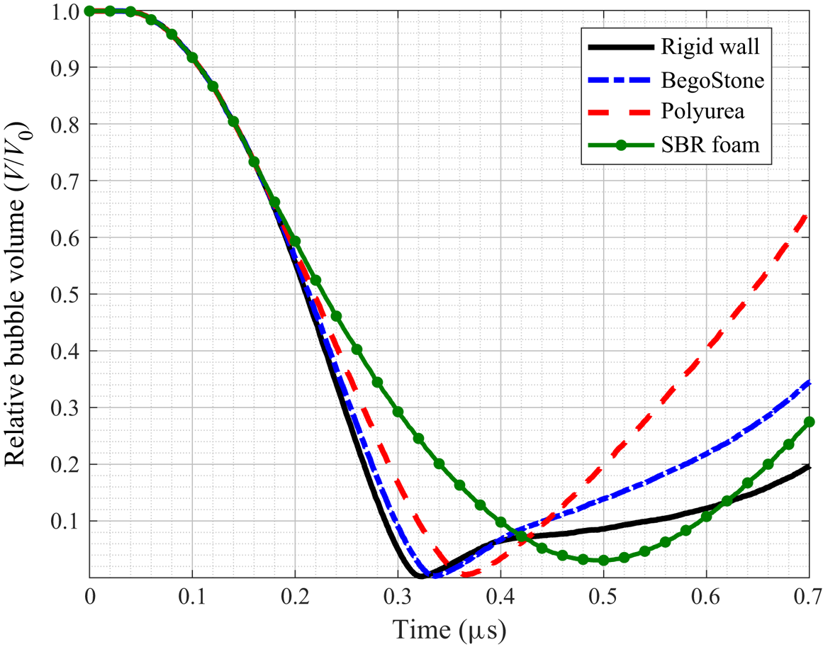
Figure 12 compares the time history of bubble volume for all the simulated cases, including the degenerate case of the same bubble collapsing near a rigid wall. The bubble's volume is initially the same in all the cases, until approximately  $0.15\ \mathrm {\mu }\text {s}$, when the reflection of the incident shock arrives at the distal side of the bubble. Afterwards, the four curves in figure 12 start to diverge, indicating a clear impact of the reflected wave. The bubble's collapse time, defined as the time between the arrival of the incident shock wave and the time the bubble reaches its minimum volume, increases from
 $0.293\ \mathrm {\mu }\text {s}$ in the case of rigid wall to
 $0.306\ \mathrm {\mu }\text {s}$ in the case of BegoStone,
 $0.335\ \mathrm {\mu }\text {s}$ in the case of polyurea, and
 $0.465\ \mathrm {\mu }\text {s}$ in the case of the foam. Also, the bubble's minimum relative volume increases in the same order from
 $2.4 \times 10^{-3}$ in the case of the rigid wall to
 $4.7 \times 10^{-2}$ in the case of the foam. Given the causal relation between the material's acoustic impedance and the type (compression or tension) and amplitude of the reflected wave, the result shown in figure 12 suggests that in the current context, a solid material with lower acoustic impedance may reduce both the energy released from bubble collapse and its peak power.
Comparison of the time history of bubble volume with different solid and soft materials in its vicinity.

When the cases of rigid wall, BegoStone, and polyurea are compared, it is interesting to note that the speed of the bubble's rebound has the opposite trend compared to that of the collapse. Specifically, the time it takes for the bubble to rebound from its minimum volume to  $1/5$ of its initial volume decreases from
 $0.38\ \mathrm {\mu }\text {s}$ in the case of rigid wall to
 $0.24\ \mathrm {\mu }\text {s}$ in the case of BegoStone and
 $0.14\ \mathrm {\mu }\text {s}$ in the case of polyurea. This trend reversal can be attributed to the reflection of the shock wave resulting from bubble collapse (i.e. the emitted shock wave) at the material surface. A material with higher acoustic impedance sends back a stronger compressive wave, which leads to slower bubble rebound.
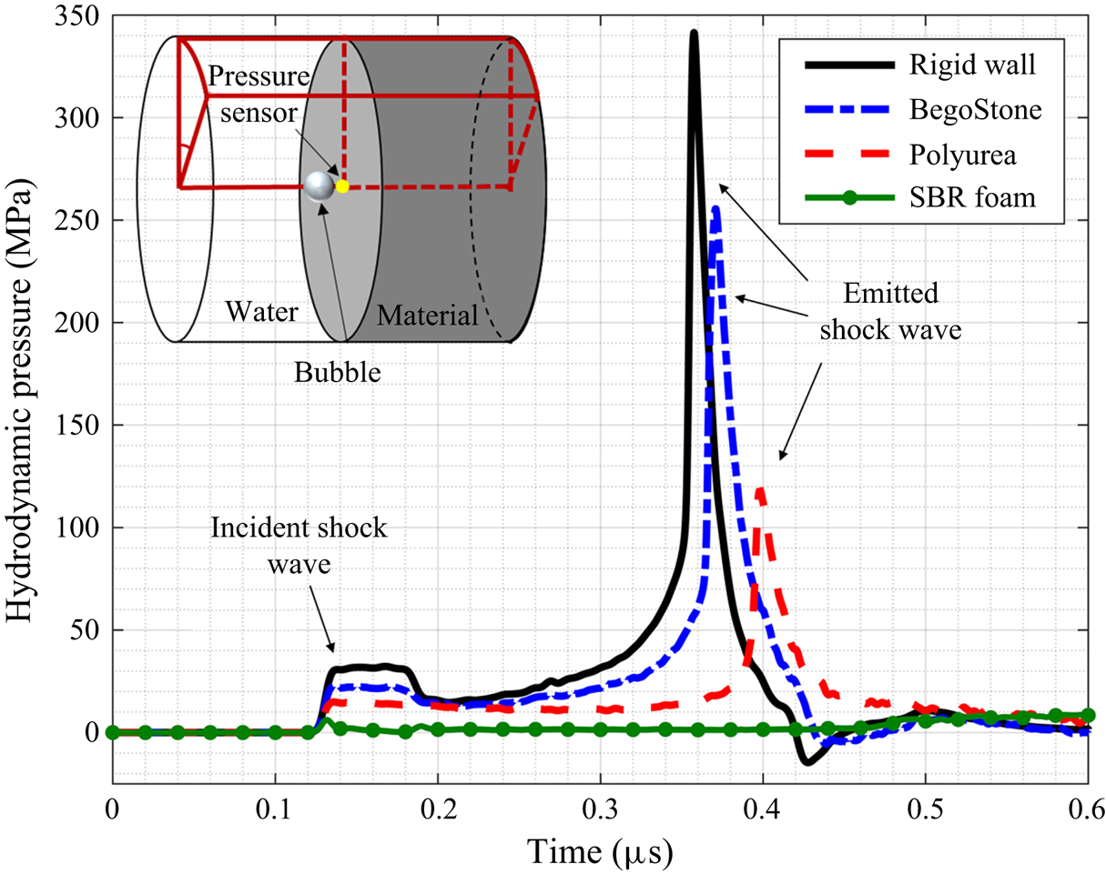
Figure 13 shows the time history of hydrodynamic pressure at the centre of the material surface. The peak pressure of the shock wave emitted from bubble collapse is  $341$ MPa in the case of rigid wall (which agrees reasonably well with the previous study of Johnsen & Colonius Reference Johnsen and Colonius2008),
 $255$ MPa in the case of BegoStone, and
 $119$ MPa in the case of polyurea. As expected, it correlates positively with the speed of bubble collapse (cf. figure 12). In all these three cases, the peak pressure value is significantly higher than the amplitude of the incident shock wave, which is
 $35\ \text {MPa}$. In the case of the foam, the bubble's collapse does not generate a shock wave. Therefore, compared to the other cases, the time history of sensor pressure in the case of the foam is nearly a flat line. The impulse of dynamic pressure at the sensor location is found to be
 $13.5$,
 $11.5$,
 $8.0$ and
 $1.5$ MPa-
 $\mathrm {\mu }$s in the case of the rigid wall, BegoStone, polyurea and the foam, respectively.
Time history of hydrodynamic pressure at a sensor on the material surface. The magnitude of the emitted shock wave becomes smaller as the material's acoustic impedance decreases. No shock wave is observed in the case of SBR foam.

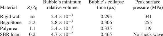
For ease of comparison, table 3 summarizes the bubble's minimum volume, collapse time and the peak surface pressure induced by the emitted shock wave in all four cases.
Comparison of the dynamics of bubble collapse near rigid wall, BegoStone, polyurea and SBR foam.

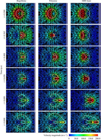
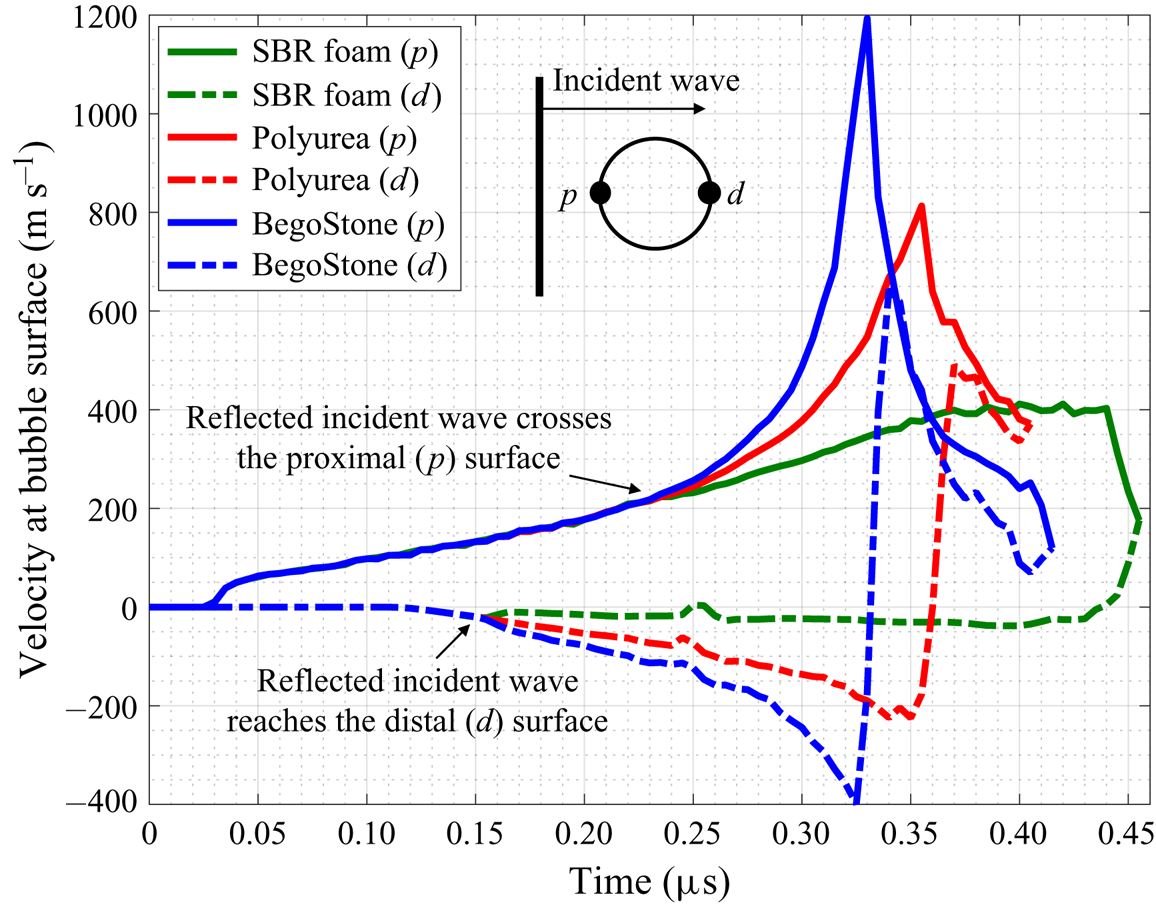
The evolution of the fluid velocity field also varies from case to case. Figure 14 shows the velocity field around the bubble during its collapse and rebound. The first row of images are taken shortly after the reflection of the incident shock passes through the bubble. Comparing the three cases shown in the figure, a variation of the speed of collapse can be observed. To clarify the difference, figure 15 compares the time history of  $x$-velocity at the proximal and distal sides of the bubble for the three materials. In the case of BegoStone, the velocity difference between the proximal and distal sides of the bubble reaches
 $1600$ m s
 $^{-1}$ shortly before contact. This is
 $1.6$ times higher than the maximum velocity observed in the case of polyurea, and
 $4$ times higher than that for the foam.
Comparison of the evolution of fluid velocity during bubble collapse and rebound, with different materials in the vicinity. Snapshots at six time instances are compared. Three supplementary movies showing the full evolution for the case of BegoStone (movie 1), Polyurea (movie 2) and SBR foam (movie 3) are available online at https://doi.org/10.1017/jfm.2020.810.

Time history of fluid velocity on the proximal ( $p$) and distal (
 $d$) sides of the bubble surface.

Figure 14 also shows the formation and evolution of the liquid jet. Comparing the three cases presented in the figure, it is notable that there is not a positive correlation between the velocity of the liquid jet and the speed of the bubble's collapse. In particular, after  $t = 0.4\ \mathrm {\mu }\text {s}$, the velocity of the jet is lower in the case of BegoStone than in the case of polyurea, despite that in the former case the bubble collapsed faster. This phenomenon is due to the reflection of the emitted shock wave at the material surface, and is essentially an effect of the material's acoustic impedance. More specifically, because of a higher acoustic impedance, BegoStone reflects a larger fraction of the incident shock wave back to the bubble (cf. figure 11,
 $t=0.155\ \mathrm {\mu }\text {s}$), which accelerates the bubble's collapse, therefore emitting a stronger shock wave at the end of the collapse (cf. figure 13). For the same reason, BegoStone sends back a stronger (compressive) reflected wave when the emitted shock wave reaches the material surface. This reflection arrives at the distal side of the bubble at
 $t = 0.4\ \mathrm {\mu }\text {s}$, when the liquid jet has just formed (figures 11 and 14). Thus the velocity of the jet is reduced due to the impact of the reflected wave. In the case of the foam, the collapse of the bubble is decelerated by the reflection of the incident wave (which is tensile, due to the material's low acoustic impedance). Therefore, as the liquid jet approaches the material surface, its velocity is higher than both of the other two cases (see the last two rows of images in figure 14). This chain reaction highlights an interaction of bubble, fluid and solid dynamics, and can be summarized by a sequence of events as below.
(a) When the incident shock wave arrives, because of the difference in acoustic impedance, BegoStone reflects a strong compressive wave to the bubble, while the foam sends back a tensile wave (figure 11,
$t=0.155\ \mathrm {\mu }\text {s}$).(b) Because of (a), the bubble in the case of BegoStone collapses much faster than the bubble in the case of the foam (figures 11 and 14,
$t\leq 0.365\ \mathrm {\mu }\text {s}$ for BegoStone, and $t\leq 0.45\ \mathrm {\mu }\text {s}$ for the foam).(c) Because of (b), the bubble in the case of BegoStone emits a strong shock wave at the end of its collapse (figure 11,
$t\leq 0.365\ \mathrm {\mu }\text {s}$), which is absent in the case of the foam (figure 11, $t\leq 0.45\ \mathrm {\mu }\text {s}$).(d) Because of (c), BegoStone sends back another compressive wave towards the bubble when the emitted shock wave arrives at its surface (figure 11,
$0.365\ \mathrm {\mu }\text {s} \leq t \leq 0.4\ \mathrm {\mu }\text {s}$). This event does not occur in the case of the foam.(e) Because of (d), the liquid jet in the case of BegoStone is decelerated (figure 14,
$0.4\ \mathrm {\mu }\text {s}\leq t \leq 0.8\ \mathrm {\mu }\text {s}$).(f) Because of (e), the jet velocity at the material surface is much lower in the case of BegoStone than in the case of the foam (figure 14,
$t=0.8\ \mathrm {\mu }\text {s}$).





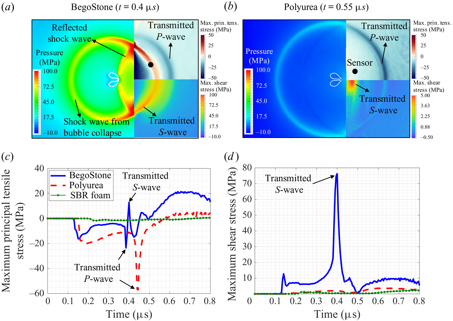
The transient stress field inside the solid material also varies from case to case. For example, figures 16(a) and 16(b) show the response of BegoStone and polyurea to the shock wave emitted from bubble collapse. For both materials, a longitudinal wave ( $P$-wave) and a transverse wave (
 $S$-wave) are captured. For BegoStone, the speeds of longitudinal and transverse waves are
 $4159$ m s
 $^{-1}$ and
 $2319$ m s
 $^{-1}$, greater than the speed of sound in water. Therefore, in figure 16(a) both waves have a crescent shape, and the longitudinal wave is clearly forward of the shock wave in water. In polyurea, the longitudinal wave travels at a speed of
 $1600$ m s
 $^{-1}$, which is close to the speed of sound in water. Hence in figure 16(b) the front of the longitudinal wave is almost aligned with the shock front at the fluid–solid interface. Also, the transverse wave in polyurea is roughly parallel to the fluid–solid interface. This is because the speed of transverse waves in polyurea is around
 $300$ m s
 $^{-1}$, much smaller than the speed of sound in water. In addition, figure 16(c,d) compares the time history of maximum principal tensile stress and maximum shear stress at a sensor, which also show clear differences among the three materials.
(a,b) Two snapshots showing different elastic waves propagating in BegoStone and the polyurea. (c,d) Time history of the maximum principal tensile stress and the maximum shear stress at a sensor located at ( $0.05$,
 $0.05$,
 $0.0$) mm.

Remark: In combination, the results of fluid pressure (figures 11 and 13) and velocity (figure 14) suggest that under the simulated condition, the primary mechanism of material damage may depend upon the material's acoustic impedance. For a ‘hard’ material with relatively high acoustic impedance, the primary mechanism may be the shock wave emitted at the end of the bubble collapse. For a ‘soft’ material with relatively low acoustic impedance, the primary mechanism appears to be the liquid jet. This finding is generally consistent with the results of some previous studies, such as Tomita & Shima (Reference Tomita and Shima1986), Shaw et al. (Reference Shaw, Schiffers, Gentry and Emmony2000), Sankin & Zhong (Reference Sankin and Zhong2006) and Abouel-Kasem et al. (Reference Abouel-Kasem, El-Deen, Emara and Ahmed2009), although the material and condition considered in each study are different.
5. Parametric study on the effects of acoustic impedance
5.1. Acoustic impedance as a key parameter
The results presented in § 4 show that the acoustic impedance of the solid material has significant impact on the bubble and fluid dynamics. A complexity, however, is that acoustic impedance is a function of the material's density and elastic properties. Specifically (see, e.g. Brekhovskikh & Godin Reference Brekhovskikh and Godin2012),
 \begin{equation} Z = \sqrt{\frac{\rho_s E(1-\nu)}{(1+\nu)(1-2\nu)}}.\end{equation}
Therefore, it is impossible to vary acoustic impedance while keeping all the other properties the same, or to fix acoustic impedance while varying only one of the other properties. Indeed, because the materials considered in § 4 are selected from real-world materials of practical importance, they differ not only in  $Z$, but also in
 $\rho _s$,
 $E$ and
 $\nu$.
To gain more insight into the role of acoustic impedance, we consider three numerical tests that involve artificial materials with prescribed properties. In each test, we fix the value of  $Z$, and vary two of the three parameters:
 $\rho _s$,
 $E$ and
 $\nu$.
(i) Test 1: shock-induced bubble collapse near a series of materials that have the same values of
$Z$ and $\rho _s$, but different values of $E$ and $\nu$.(ii) Test 2: shock-induced bubble collapse near a series of materials that have the same values of
$Z$ and $\nu$, but different values of $\rho _s$ and $E$.(iii) Test 3: shock-induced bubble collapse near a series of materials that have the same values of
$Z$ and $E$, but different values of $\rho _s$ and $\nu$.


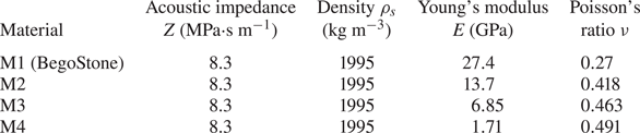
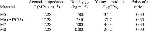
In Test 1, we consider four materials as shown in table 4, including BegoStone. Their Young's modulus and Poisson's ratio vary by a factor of  $16$ and
 $1.8$, respectively. For each material, we perform the numerical analysis described in § 4.1, using the same computational model.
Test 1 material properties.

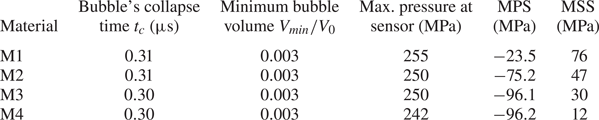
Table 5 summarizes the results obtained from Test 1, including the bubble's collapse time ( $t_{c}$), the minimum bubble volume (
 $V_{min}/V_{0}$), the maximum pressure at the sensor shown in figure 13 and the maximum values of maximum principal and shear stresses at the sensor shown in figure 16. The table shows that when
 $Z$ and
 $\rho _s$ are fixed, the bubble and fluid dynamics are relatively insensitive to variation in
 $E$ or
 $\nu$. The small changes can be explained by the fact that while the material's density and longitudinal wave speed are fixed, the transverse wave speed does vary among the four materials. For the same reason, it is not surprising that the stress field inside the material clearly varies among the four cases.
Test 1 results.

MPS and MSS: the temporal maximum of maximum principal stress and maximum shear stress at the sensor shown in figure 16. For MPS, the negative (i.e. compressive) peak is shown.
In the same way, we perform Test 2 for the materials shown in table 6, in which  $\rho _s$ varies from
 $1500$ to
 $10\ 000\ \text {kg}\ \text {m}^{-3}$, and
 $E$ from
 $20.2$ to
 $134.4\ \text {GPa}$. The result shows that
 $t_c$ varies by less than
 $1\,\%$, from
 $0.298$ to
 $0.300\ \mathrm {\mu }\text {s}$;
 $V_{min}/V_{0}$ varies by around
 $3\,\%$, from
 $0.00275$ to
 $0.00285$. The maximum sensor pressure varies by around
 $5\,\%$, from
 $280$ to
 $296$ MPa. In comparison, variation in the material's stress field is much larger. For example, at the aforementioned sensor location (figure 16), the peak value of maximum shear stress varies from
 $121.4$ to
 $200.1\ \text {MPa}$.
Test 2 material properties.

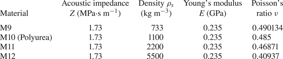
In Test 3, we consider the four materials shown in table 7. The material's acoustic impedance and Young's modulus are fixed, and their density and Poisson's ratio vary by a factor of  $7.5$ and
 $1.2$, respectively. Again, the fluid results are relatively insensitive to the material variations. For example, the peak pressure at the aforementioned sensor location varies by
 ${\sim }5\,\%$, from
 $119$ to
 $125\ \text {MPa}$.
Test 3 material properties.

Combining the results of the above numerical tests and those presented in § 4, it is evident that under the simulated conditions, the solid material's acoustic impedance ( $Z$) is an important parameter that controls the material's reciprocal effect to the two-phase fluid flow. The same bubble collapsing near materials with different values of
 $Z$ can produce clearly different bubble and fluid dynamics, with
 $Z=Z_0$ being a transition point. On the other hand, the same bubble collapsing near materials that have the same value of
 $Z$, yet differ in other elastic properties, are found to produce similar bubble and fluid dynamics (yet dissimilar stress field inside the material).
5.2. Selection of materials with different values of acoustic impedance
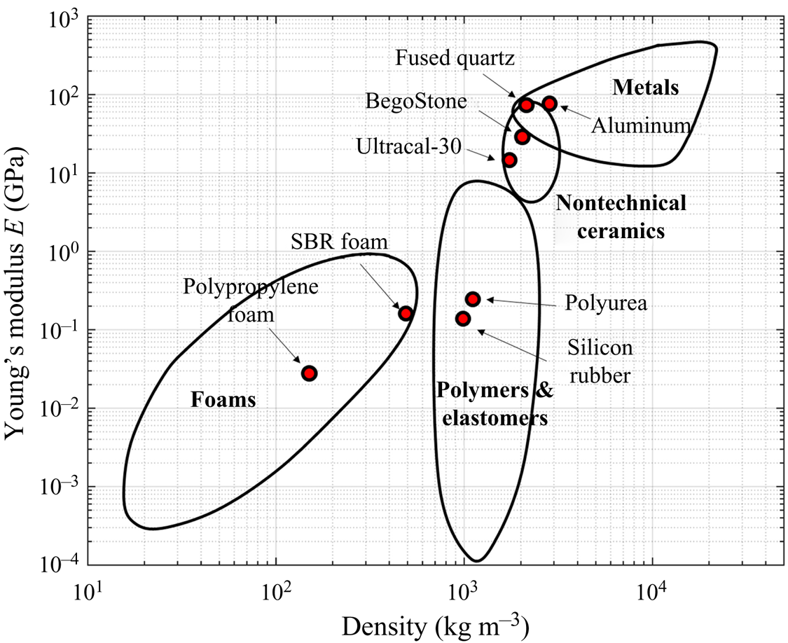
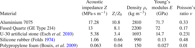
To characterize the effect of acoustic impedance on bubble and fluid dynamics, we select five additional materials with acoustic impedance varying in a broader range compared to those considered in § 4. The materials are selected from several broad categories, as shown in figure 17. Table 8 summarizes the properties of these materials. In particular, their acoustic impedance varies from  $0.063$ to
 $17.28$ MPa
 $\cdot$s m
 $^{-1}$. For each material, we conduct the same numerical analysis described in § 4.1.
Selected materials for parametric study (the Young's modulus–density diagram is adapted from Ashby Reference Ashby2010).

Properties of five additional materials with different acoustic impedance.

In the following, we combine the new materials in table 8 with those considered in § 4 (table 2), and characterize the effect of acoustic impedance on three fluid quantities of interest, namely the bubble's collapse time, the minimum bubble volume and the maximum hydrodynamic pressure on the material surface.
5.3. Effect of acoustic impedance on bubble collapse time
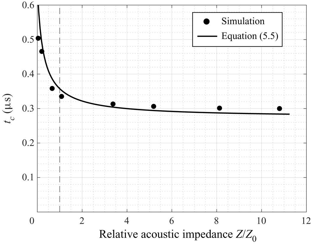
Figure 18 shows in black dots the bubble's collapse time,  $t_c$, for the eight materials considered. As the material's acoustic impedance increases,
 $t_c$ decreases monotonically. This trend is consistent with what we found in § 4 using the three representative materials, and has been explained there. The dashed line in figure 18 marks
 $Z/Z_0=1$. For materials with
 $Z/Z_{0}>1$, the variation in
 $t_c$ is relatively small. For example, as
 $Z/Z_{0}$ decreases from
 $10.8$ (aluminium) to
 $1.1$ (polyurea),
 $t_c$ increases by
 $10\,\%$. When
 $Z/Z_{0}<1$,
 $t_c$ becomes more sensitive to
 $Z$. It increases from
 $0.36\ \mathrm {\mu }\text {s}$ in the case of the rubber (
 $Z/Z_{0}=0.66$) to
 $0.465\ \mathrm {\mu }\text {s}$ in the case of the SBR foam (
 $Z/Z_{0}=0.2$).
Effect of material's acoustic impedance on the bubble's collapse time. Dashed line:  $Z=Z_0$.

The trend shown in figure 18 can be captured using a simple model. We recall that in the case of free-field Rayleigh collapse modelled by the Rayleigh–Plesset equation, after neglecting the gas content inside the bubble, the collapse time can be derived as (Brennen Reference Brennen2014)
 \begin{equation} t_{c}^{R} = 0.915 \sqrt{\frac{\rho_{l}}{p_{\infty}-p_{v}}} R_{0},\end{equation}
in which the superscript R denotes Rayleigh collapse;  $\rho _l$ denotes the density of the liquid,
 $p_\infty$ the far field pressure,
 $p_v$ the vapor pressure and
 $R_0$ the initial bubble radius. Further, for the non-spherical Rayleigh collapse of a bubble near a rigid wall, Rattray (Reference Rattray1951) proposed that the bubble's collapse time can be approximated by
 \begin{equation} t_{c}^{R,w} \approx t_{c}^{R} \left( 1+0.205 \frac{R_{0}}{D_{0}} \right) = 0.915 \sqrt{\frac{\rho_{l}}{p_{\infty}-p_{v}}} R_{0} \left( 1+0.205 \frac{R_{0}}{D_{0}} \right), \end{equation}
where the superscript w on  $t_c$ denotes wall, and
 $D_0$ is the distance between the centre of the bubble to the wall (cf. Johnsen & Colonius Reference Johnsen and Colonius2009; Koch et al. Reference Koch, Lechner, Reuter, Köhler, Mettin and Lauterborn2016).
In the present study, the bubble's collapse is induced by a shock wave, which is different from a uniform pressure  $p_\infty$ in Raleigh collapse. Moreover, in § 4 we have shown that the bubble's collapse time depends sensitively on both the incident shock and its reflection against the material surface, while the amplitude of the reflected wave is a function of
 $Z/Z_0$. Therefore, we replace
 $p_\infty$ in (5.3) by
 \begin{equation} p_s = p_i + c_r p_r = p_i \left(1 + c_r \frac{Z/Z_0 - 1}{Z/Z_0 + 1}\right), \end{equation}
where  $p_i$ is a characteristic pressure of the incident shock,
 $p_r$ the pressure of its reflection ((4.1)), and
 $c_r$ a non-dimensional coefficient that accounts for the time lag between the impact of the incident shock wave and that of the reflected wave. In other words, we propose that for the current study, the bubble's collapse time can be described by
 \begin{equation} t_{c} = 0.915 \sqrt{\frac{\rho_{l}}{p_{i} \left( 1 + c_{r}\dfrac{Z/Z_0 - 1}{Z/Z_{0} + 1} \right) - p_{v}}} R_{0} \left( 1+0.205\dfrac{R_{0}}{D_{0}} \right).\end{equation}
The solid line in figure 18 shows the prediction of the above model, with  $p_i = 20\ \text {MPa}$ (approximately half of the peak pressure of the incident shock) and
 $c_r=0.7$. It agrees well with the result of the numerical analysis.
5.4. Effect of acoustic impedance on minimum bubble volume
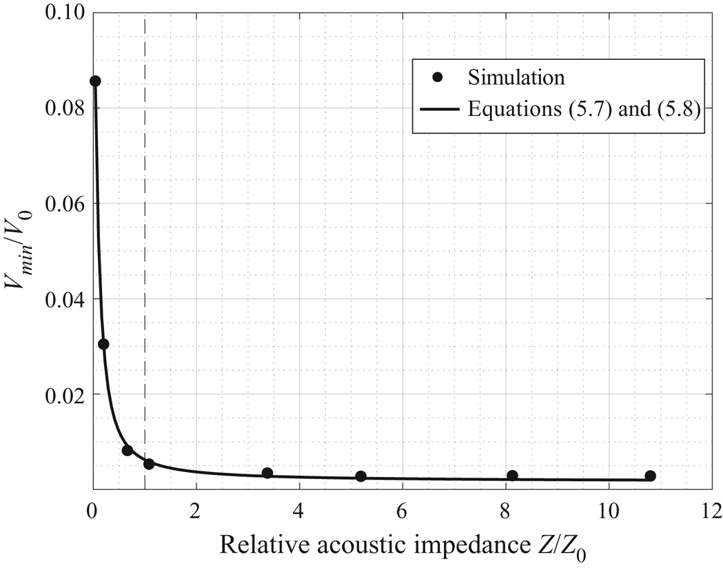
In figure 19, the black dots show the bubble's minimum volume normalized by its initial volume, i.e.  $V_{min}/V_{0}$, for the eight materials considered. As the material's acoustic impedance increases,
 $V_{min}/V_0$ decreases monotonically. The trend is nonlinear and again,
 $Z/Z_0=1$ roughly marks a turning point. The minimum bubble volume is more sensitive to the nearby material's acoustic impedance when
 $Z/Z_{0} < 1$. For example,
 $V_{min}/V_{0}$ in the case of polypropylene foam (
 $Z/Z_{0} = 0.04$) is more than
 $9$ times higher than that in the case of rubber (
 $Z/Z_{0} = 0.66$). In comparison, the difference between the case of Ultracal-30 stone (
 $Z/Z_{0} = 3.4$) and the case of aluminium (
 $Z/Z_{0} = 10.8$) is less than
 $20\,\%$.
Effect of material's acoustic impedance on the bubble's minimal volume. Dashed line:  $Z=Z_0$.

The effect of acoustic impedance on minimum bubble volume can also be captured using a phenomenological model derived from the Rayleigh–Plesset equation. Again, we recall that in the case of free-field Rayleigh collapse modelled by the Rayleigh–Plesset equation, the minimum bubble volume can be derived analytically (Brennen Reference Brennen2014). After neglecting surface tension, we have
 \begin{equation} R^{R}_{min} = R_{0} \left[ \frac{p_{G_0}}{(\gamma_{G}-1) \left( p_{\infty}-p_{v} \right)} \right]^{1/[3(\gamma_{G}-1)]},\end{equation}
where  $R_{min}^R$ denotes the minimum radius of the bubble, which is assumed to remain spherical all the time. Again, the superscript
 $R$ denotes Rayleigh collapse;
 $p_{G_0}$ denotes the partial pressure of gas inside the bubble;
 $p_v$ denotes the vapor pressure; and
 $\gamma _G$ the specific heat ratio of the internal gas.
To account for non-spherical collapse, we generalize the definition of bubble radius ( $R$) as
 \begin{equation} R = \left( \frac{V}{4 {\rm \pi}/3} \right)^{1/3}. \end{equation}
Then, we generalize the above analytical result from Rayleigh–Plesset equation in the same way described in § 5.3, which gives
 \begin{equation} R_{min} = R_{0} c_{s} \left[ \frac{p_{0}}{(\gamma_{G}-1)\left[ p_{i} \left( 1+c_{r}\displaystyle \frac{Z-Z_{0}}{Z+Z_{0}} \right) - p_{v} \right]} \right]^{1/[3(\gamma_{G}-1)]}.\end{equation}
The solid line in figure 19 shows the minimum bubble volume predicted by (5.8) with  $p_i=20\ \text {MPa}$,
 $c_{r}=0.7$ and
 $c_{s}=7.0$. The prediction agrees well with the result of numerical analysis.
5.5. Effect on the maximum pressure on material surface
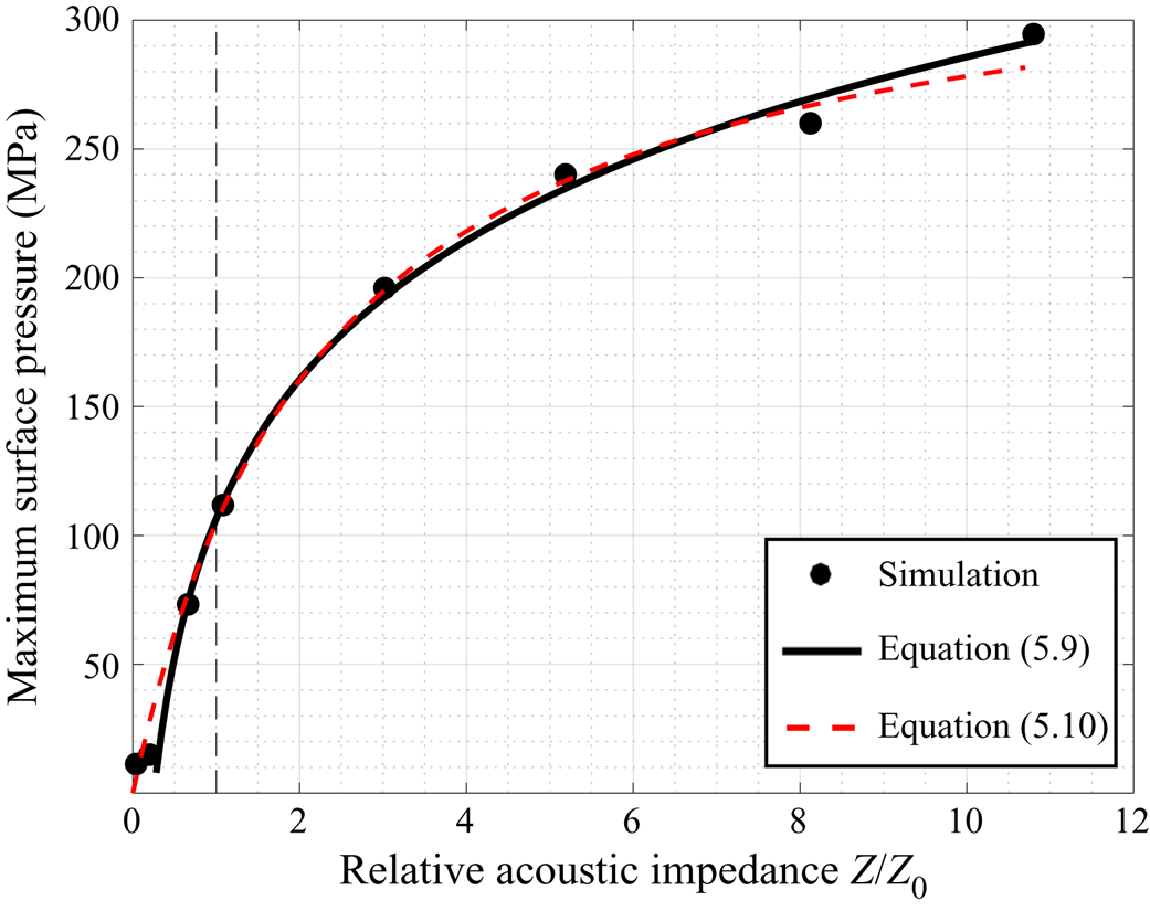
Figure 20 shows in black dots the maximum hydrodynamic pressure on the material surface, denoted by  $p_{{w,max}}$, for the eight materials considered. Again, a monotonic relationship is observed. Specifically, as
 $Z/Z_0$ varies from
 $0.04$ (in the case of the polypropylene foam) to
 $10.8$ (in the case of aluminium 7075),
 $p_{{w,max}}$ increases by
 $26$ times, from
 $11.3$ to
 $291.6$ MPa. The increase of maximum pressure is nonlinear with respect to
 $Z/Z_0$, and the slope reduces as the acoustic impedance becomes larger (i.e. concave). It can be expected that as
 $Z/Z_{0}$ goes to infinity,
 $p_{{max}}$ would approach the value obtained from the case with a rigid wall (cf. figure 13).
Effect of material's acoustic impedance on the maximum hydrodynamic pressure on material surface. Dashed line:  $Z=Z_0$.

For the eight materials considered (with  $Z/Z_{0} \in [0.04,10.8]$),
 $p_{{w,max}}$ is approximately a linear function of
 $\log (Z/Z_{0})$. Using least-squares fitting, the relationship is given by
 \begin{equation} p_{{w,max}}^{(1)} = \rho c_{0}^2 \left[ 0.07 \log_{10}\left( \frac{Z}{Z_{0}} \right) + 0.0416 \right], \end{equation}
where  $c_0$ denotes the speed of sound in the fluid. This fitting function is plotted in figure 20. Despite the simplicity, a linear function like (5.9) cannot capture the correct asymptotic behaviour as
 $Z/Z_0$ goes to infinity. Accounting for the case of
 $Z/Z_0=\infty$ (i.e. a rigid wall), we find that
 $p_{{w,max}}$ can also be fitted using a bounded growth function,
 \begin{equation} p_{{w,max}}^{(2)} = \rho c_{0}^2 \frac{0.0591(Z/Z_0)}{1+0.4434(Z/Z_0)},\end{equation}
which is also shown in figure 20.
5.6. Effect of bubble's stand-off distance
While the material's acoustic impedance dictates the reflection of shock wave at the material surface, the bubble's stand-off distance determines the time when the reflected shock waves reach and interact with the bubble, and hence, is an important parameter that affects the subsequent bubble dynamics. To study how the stand-off distance  $D_{0}$ influences the material's reciprocal effects discussed above, we re-run the three representative cases presented in § 4 using different
 $D_{0}$ between
 $R_{0}$ and
 $6R_{0}$.
Table 9 compares the results obtained with a stand-off distance of  $D_{0} = 4 R_{0}$ and the results for
 $D_{0} = 2R_{0}$ from table 3. For both stand-off distances, similar trends in bubble's collapse time and the peak surface pressure with respect to
 $Z/Z_{0}$ can be observed. However, the differences between three materials in the case of
 $D_{0} = 4R_{0}$ becomes smaller, indicating that the effect of nearby materials becomes weaker with increased stand-off distance. This is because it takes longer (i.e. approximately twice as the case of
 $D_{0} = 2R_{0}$) for the reflected wave to reach and interact with the collapsing bubble, which thus weakens the material's effect on the collapse process. Another interesting observation is that because of the reduced effect from the nearby material, a shock wave is emitted in the case of the SBR foam with
 $D_{0} = 4R_{0}$.
Comparison of the dynamics of bubble collapse with two stand-off distances ( $D_{0} = 2 R_{0}$ and
 $D_{0} = 4 R_{0}$).

Furthermore, there exists a limit value of standoff distance, above which the bubble would reach its minimum volume before the reflection of the incident shock arrives, therefore its initial collapse is not affected by the solid material. Our numerical test suggests that for the current setting, the limit stand-off distance is approximately  $D^{*}_{0} = 5.5R_{0}$.
We also find that (5.5) provides a good estimate of this limit stand-off distance. Specifically, the time for the shock wave to travel between the bubble and the material surface (back and forth) is given by
 \begin{equation} t_{wp} = \frac{2D_{0}}{c} = 2D_{0} \sqrt{\frac{\rho_{l}}{\gamma_{L} (p+p_{L})}} \approx 2D_{0} \sqrt{\frac{\rho_{l}}{\gamma_{L} p_{L}}},\end{equation}
where  $D_{0}$ denotes the bubble's stand-off distance,
 $\gamma _{L}$ and
 $p_{L}$ are constant coefficients of the stiffened equation of state. At the limit stand-off distance, denoted by
 $D^{*}_{0}$,
 $t_{wp}$ is equal to the bubble's collapse time,
 $t_{c}$. Combining (5.5) with
 $c_{r} = c^{*}_{r} = 0$ and (5.11) gives
 \begin{equation} 2D^{*}_{0} \sqrt{\frac{\rho_{l}}{\gamma_{L} p_{L}}} = 0.915 \sqrt{\frac{\rho_{l}}{p_{i}-p_{v}}} R_{0} \left( 1+0.205 \frac{R_{0}}{D^{*}_{0}} \right) \end{equation}
which is a quadratic equation of  $R_{0}/D^{*}_{0}$. Solving this equation gives
 $R_{0}/D^{*}_{0} = 0.1809$, or equivalently,
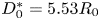 $D^{*}_{0}=5.53 R_{0}$, which matches well the result of our numerical test.
6. Summary and conclusions
Using a recently developed fluid–solid coupled computational model, we have analysed the collapse of a single bubble induced by a shock wave near different types of solid materials, including metals, minerals, glass, polymers and foams. By coupling the dynamics of the bubble, the ambient liquid, and the solid material, the computational model allowed us to investigate their interactions in detail. In this study, we have focused on elucidating the effects of the solid material's longitudinal acoustic impedance ( $Z$) on the bubble and fluid dynamics, including the shock wave and liquid jet resulting from the bubble's collapse. We presented a detailed comparison of three representative cases with
 $Z/Z_0>1$,
 $Z/Z_0\approx 1$, and
 $Z/Z_0<1$, respectively, where
 $Z_0$ is the acoustic impedance of the ambient fluid (water). Then, we expanded the study with five additional materials to cover a relatively broad range of
 $Z/Z_0$, that is, between
 $0.04$ and
 $10.8$. We investigated the effects of
 $Z/Z_0$ on the bubble's collapse time, the minimum bubble volume and the maximum hydrodynamic pressure on the material surface. We also designed and calibrated phenomenological models to capture these effects.
Several main findings of this study are noteworthy. First, the study reveals a two-way coupling between the fluids and the solid material: when the same bubble collapses near different materials (especially, materials with different acoustic impedance), the stress field inside the material, the bubble dynamics, the fluid pressure and velocity fields and the shock wave and liquid jet resulting from the bubble's collapse all vary. This finding indicates that modelling a material surface as a rigid wall may be inaccurate, even if the solid material has a Young's modulus on the order of tens of GPa. (see, e.g. figure 13). Second, the study shows that  $Z/Z_0$ is a key parameter that dominates the material's reciprocal effect to the bubble and fluid dynamics, including the speed of bubble collapse and rebound, the speed of the liquid jet, and the emission (and amplitude) of the shock wave resulting from bubble collapse. This finding is supported both by a mechanistic study on the three representative cases with different values of
 $Z$, and a numerical parametric study of materials that have the same
 $Z$, yet differ in density, Young's modulus and Poisson's ratio. Third, the study shows that
 $Z/Z_0=1$ can be considered as a transition point. When
 $Z/Z_0<1$, the material surface reflects the compressive front of the incident shock wave as a tensile wave. The reflection reduces the speed of the bubble's collapse. As a result, the collapse produces a liquid jet, but not necessarily a shock wave. When
 $Z/Z_0>1$, the surface reflects the compressive shock front as a compressive wave. The reflection accelerates the bubble's collapse. As a result, the maximum pressure of the emitted shock wave increases linearly with
 $\log (Z/Z_0)$ (within the range mentioned above), and can be much higher than the amplitude of the incident shock. Interestingly, this emitted shock wave also gets reflected at the material surface, and the reflected wave slows down the liquid jet. More generally, this finding indicates that the mechanisms of cavitation-induced material damage may be related to the material's acoustic impedance. For materials with high acoustic impedance, our study indicates that the emitted shock wave may have a peak pressure of the order of
 $100\ \text {MPa}$. But for ‘soft’ materials with
 $Z<Z_0$, the bubble's collapse may not emit a shock wave. Instead, the high-speed liquid jet may become a mechanism of material damage.
A few limitations of this study should also be mentioned. The study considers a specific setting that features the collapse of an air bubble induced by a planar shock wave, while the viscous/viscoelastic effects of the surrounding liquid on the bubble collapse are neglected. The generality of the findings obtained for this setting – particularly, their validity under different conditions – requires further investigation. Also, although we commented on the mechanisms of cavitation-induced material damage based on the fluid pressure and velocity results, the numerical simulations do not directly predict material damage or fracture. Incorporation (and calibration) of material damage and fracture models is non-trivial, but possible (see, e.g. Cao et al. Reference Cao, Zhang, Liao, Zhong and Wang2019). Furthermore, the phenomenological models proposed in § 5 can be generalized – for example,  $c_s$ and
 $c_r$ should be functions of the bubble's stand-off distance. In our opinion, these are all worthwhile directions for future study.
Acknowledgements
The authors gratefully acknowledge the support of the National Science Foundation (NSF) under Awards CBET-1751487 and CBET-1706003, and the support of the Office of Naval Research (ONR) under Awards N00014-17-1-2831 and N00014-19-1-2102. The authors thank Drs Y. Zhang, Q. Zhan, and P. Zhong for their advice and assistant on the verification study, and Drs P. Avery and C. Farhat for their advice and assistance on the development and use of the computational model.
Declaration of interests
The authors report no conflict of interest.
Supplementary movies
Supplementary movies are available at https://doi.org/10.1017/jfm.2020.810.