


1. Introduction
Temperature gradients along the interface between two immiscible fluids cause variations of surface tension resulting in tangential stresses which can drive bulk flow motion. An increase in the temperature gradient leads to instability of the thermocapillary flow. Smith & Davis (Reference Smith and Davis1983a,Reference Smith and Davisb) employed a linear theory to investigate the stability of the thermocapillary flow (also called Marangoni convection) for two different planar geometries: an infinite liquid layer (the linear flow) and a two-dimensional slot (the return flow). Two classes of thermal-convective instabilities were found: stationary longitudinal rolls and propagating hydrothermal waves (HTWs). In the return-flow configuration a HTW propagates at angles with respect to the direction of the surface flow that depend on the Prandtl number of the fluid. The Prandtl number  $Pr=\nu /\chi$ is defined as the ratio between the kinematic viscosity
 $\nu$ and the thermal diffusivity
 $\chi$ of the fluid.
Interest in Marangoni convection sharply rises starting from the early 1980s, driven by the possibility to conduct experiments in microgravity (Schwabe Reference Schwabe2014) where other types of convection are absent. A promising direction was the growth of high-quality crystals in space, which sparked interest for studies of Marangoni convection in cylindrical geometry, in particular, in liquid bridges (LBs) serving as a model for the floating zone technique. A LB is a droplet of fluid suspended between two concentric disks maintained at different temperatures  $T_{hot}$ and
 $T_{cold}$. At a small temperature difference, the flow is a steady axisymmetric toroidal vortex. For most of the liquids, the temperature dependence on surface tension is negative and this causes a flow directed along the interface from hot to cold parts of a liquid.
When  ${\rm \Delta} T = T_{hot}-T_{cold}$ exceeds a critical value
 ${\rm \Delta} T_{cr},$ instability sets in as the result of Hopf bifurcation and gives rise to a number of time-dependent three-dimensional flow regimes (Kuhlmann Reference Kuhlmann1999; Lappa Reference Lappa2010). In particular, instability may generate standing or travelling HTWs or lead to temporally chaotic dynamics (Ueno, Tanaka & Kawamura Reference Ueno, Tanaka and Kawamura2003; Melnikov, Shevtsova & Legros Reference Melnikov, Shevtsova and Legros2004; Matsugase et al. Reference Matsugase, Ueno, Nishino, Ohnishi, Sakurai, Matsumoto and Kawamura2015). A travelling wave (TW) can propagate in the azimuthal (Wanschura et al. Reference Wanschura, Shevtsova, Kuhlmann and Rath1995; Leypoldt, Kuhlmann & Rath Reference Leypoldt, Kuhlmann and Rath2000; Lappa, Savino & Monti Reference Lappa, Savino and Monti2001) or axial (Melnikov & Shevtsova Reference Melnikov and Shevtsova2009) direction and be characterized by a single integer azimuthal wavenumber
 $m$ or a combination thereof (Shevtsova, Melnikov & Legros Reference Shevtsova, Melnikov and Legros2003; Shevtsova, Melnikov & Nepomnyashchy Reference Shevtsova, Melnikov and Nepomnyashchy2009). For the first time, the oscillatory flows observed in LB experiments were associated with the concept of HTWs by Kuhlmann & Rath (Reference Kuhlmann and Rath1993). It should be emphasized that these regimes with integer azimuthal wavenumbers are not specific to the thermocapillary instability in general. Rather, they are typical representatives of flows occurring in the cylindrical geometry as a result of bifurcations breaking the axial symmetry.
The first experiments controlling ambient conditions around a LB (Kamotani et al. Reference Kamotani, Wang, Hatta, Wang and Yoda2003; Mialdun & Shevtsova Reference Mialdun and Shevtsova2006; Irikura et al. Reference Irikura, Arakawa, Ueno and Kawamura2007; Watanabe et al. Reference Watanabe, Melnikov, Matsugase, Shevtsova and Ueno2014) indicated that heat exchange between the liquid and the ambient gas is an important factor that influences the instability mechanisms. However, in numerical studies, in order to optimize the computing time the problem is typically modelled as a single-phase liquid flow when the gas phase next to the LB is ignored, assuming that the viscosity and thermal conductivity of the gas are negligible. In a one-phase model the interfacial heat transfer is neglected or, if considered, assumed in the form of Newton's law. The heat flux can be set directly (Motegi, Kudo & Ueno Reference Motegi, Kudo and Ueno2017) or, more often, through the Biot number and the temperature jump between the free surface and the reference temperature. The Biot number is defined as  $Bi=h\,R/\lambda$, where
 $h$ is the heat transfer coefficient,
 $R$ is the linear scale,
 $\lambda$ is the thermal conductivity of the liquid. In most cases, the reference temperature in the gas phase is taken to be a constant.
The role of the reference (gas) temperature distribution was examined by Melnikov & Shevtsova (Reference Melnikov and Shevtsova2014) (nonlinear simulations) and Xun et al. (Reference Xun, Kai, Hu and Imaishi2011) (linear stability analysis) considering stability of a LB with  $Pr=16\text {--}18$ and the aspect ratio
 $\varGamma =d/R_0=1.8$ (here
 $d$ is the height and
 $R_0$ is the radius of the LB). They studied three cases: two with a constant gas temperature, equal either to the temperature of the cold rod
 $T_{cold}$ or to the mean temperature of the liquid
 $T_{mean}$, and a third one with a linear temperature distribution in the gas. They both reported that the threshold of oscillatory instability and the critical wavenumber depend not only on the Biot number but also on the temperature distribution in the gas phase. It was reported that in the range of a small Biot number,
 $Bi<0.5,$ the critical wavenumber is
 $m=0$ for all temperature distributions, while with an increase in
 $Bi$ the critical wavenumber becomes
 $m=1$, and the change of that critical mode is slightly delayed in the case when the gas temperature is
 $T_{mean}$.
In practice, it is not always easy to determine the Biot number. Often, the two-phase problem is solved in the axisymmetric case with low computational costs, and the  $Bi$ number is determined from the heat flux through the interface. Then this value can be used in single-phase three-dimensional numerical simulations, and for comparison with experimental results. In this approach either the local (Kamotani et al. Reference Kamotani, Wang, Hatta, Wang and Yoda2003; Romano & Kuhlmann Reference Romano and Kuhlmann2019) or average Biot numbers (Kamotani et al. Reference Kamotani, Wang, Hatta, Wang and Yoda2003; Gaponenko & Shevtsova Reference Gaponenko and Shevtsova2012; Yano, Hirotani & Nishino Reference Yano, Hirotani and Nishino2018) are determined from the heat flux through the interface. Romano & Kuhlmann (Reference Romano and Kuhlmann2019) performed a series of calculations (
 $Pr = 28$) determining the local
 $Bi$ number, and proposed a fifth-order polynomial fit including a large set of coefficients that are tabulated and freely accessible. However, this is a very specific set of data that cannot be of wide interest due to the complexity of multi-parametric handling.
Subsequent experimental studies related to the influence of ambient conditions were focused on understanding the effect of a controlled gas flow in the annular gap between a LB and the external cylindrical tube. The gas stream can affect the stability of a flow via shear stresses, heat transfer and interface deformation. The group of Ueno (see in the survey by Shevtsova et al. Reference Shevtsova, Gaponenko, Kuhlmann, Lappa, Lukasser, Matsumoto, Mialdun, Montanero, Nishino and Ueno2014) measured the onset of instability in a LB ( $Pr=28$) with upward and downward gas flow at various aspect ratios and moderate gas velocity (
 $Re_{gas}\leqslant 100$). They reported that at the aspect ratio
 $\varGamma =1$, the gas moving downward stabilized the thermocapillary flow, while the gas moving upward had a limited effect, regardless of the aspect ratio. With a decrease in the aspect ratio, the effect of the gas moving from the hot side (downward) diminished. The Kuhlmann group performed three-dimensional linear stability analysis (LSA) of a two-phase system (
 $Pr=68$) where gravity is absent (see in Shevtsova et al. Reference Shevtsova, Gaponenko, Kuhlmann, Lappa, Lukasser, Matsumoto, Mialdun, Montanero, Nishino and Ueno2014). In general, the trends predicted in the simulations were observed in the experiments.
Particular attention to the role of viscous shear was given in the numerical analysis by Shevtsova, Gaponenko & Nepomnyashchy (Reference Shevtsova, Gaponenko and Nepomnyashchy2013) considering axisymmetric flows in LB with  $Pr=12$ and 68 with relatively high velocities of the ambient gas flow, up to
 $2\ \textrm {m}\ \textrm {s}^{-1}$, i.e.
 $Re_{gas}<600$. In the case when the gas stream comes from the cold side (upward), a new oscillatory instability was found in the form of an axially TW propagating from the hot to the cold end of the LB. The evolution of the axisymmetric flows structure in LB with
 $Pr=105$ under high gas velocity, up to
 $3\ \textrm {m}\ \textrm {s}^{-1}$, i.e.
 $Re_{gas}<900$, was recently examined by Liang et al. (Reference Liang, Jin, Yang, Shi and Zhang2020).
For statically deformed LBs, the stability diagram ( ${\rm \Delta} T$ vs
 ${\mathcal {V}}$) consists of two branches with a vertex at a certain volume ratio (Hu et al. Reference Hu, Shu, Zhou and Tang1994). The impact of a gas flow on the stability of statically deformed LBs was experimentally examined by Yano et al. (Reference Yano, Maruyama, Matsunaga and Nishino2016) for
 $Pr=28$, 67 when
 $Re_{gas}<50$, and it showed that the gas moving upward (downward) shifts the vertex position to the side of the smaller (larger) volume ratio. As for the dynamic interface deformation, it was obtained in several numerical (Herrada et al. Reference Herrada, Lopez-Herrera, Vega and Montanero2011) and experimental (Matsunaga et al. Reference Matsunaga, Mialdun, Nishino and Shevtsova2012; Yang et al. Reference Yang, Liang, Wang, Gao, Ma, Xu and Xia2018) studies that the interface deformation does not exceed
 $10\ \mathrm {\mu }\textrm {m}$ in a millimetric LB when the velocity of gas is as large as
 $2\ \textrm {m}\ \textrm {s}^{-1}$. Recent results of linear stability analysis of a LB with high Prandtl number,
 $Pr = 68$, presented by Carrión, Herrada & Montanero (Reference Carrión, Herrada and Montanero2020) showed that dynamic free surface deformation has very little effect on the stability of the flow.
The above experiments had no control over gas temperature. The first experiments controlling the temperature of a moving gas, by Yasnou et al. (Reference Yasnou, Gaponenko, Mialdun and Shevtsova2018), revealed its impact on the stability of LB with  $Pr=14$. The authors found that heat transfer is the prevailing mechanism by which gas affects the flow in a liquid. Surely, the viscous shear is present, but the liquid/gas viscosity ratio is large,
 $\mu _l/\mu _g\sim 50$, and the effect of shear stress is not overly significant for the considered velocities (
 $Re_{gas}=120$), especially when the heat transfer is important. The experimental results by Yasnou et al. (Reference Yasnou, Gaponenko, Mialdun and Shevtsova2018) converge with the previous experimental studies controlling the temperature of gas, although without forced gas motion for LB with
 $Pr=28$ and 67 (Yano et al. Reference Yano, Maruyama, Matsunaga and Nishino2016). For value of the Prandtl number within the range 14 to 68, the dependence of the critical temperature difference (
 ${\rm \Delta} T_{cr}$) on the average heat flux shows a sharp spike with a near-vertical increase and decrease. Being expressed by the Biot number it occurs within the narrow segment of
 $Bi=0.33\text {--}0.40$. This extremum was attributed to the change of azimuthal mode or flow stabilization in the case of moving gas.
The two-phase studies mentioned above are associated with the microgravity experiment JEREMI (Japanese European Research Experiment on Marangoni Instabilities). One of the objectives is to study the effect of an external coaxial gas stream on the Marangoni convection in LBs (Shevtsova et al. Reference Shevtsova, Gaponenko, Kuhlmann, Lappa, Lukasser, Matsumoto, Mialdun, Montanero, Nishino and Ueno2014). Several LB experiments have recently been conducted on the International Space Station (ISS) in the Japanese module KIBO (Sato et al. Reference Sato, Ueno, Kawamura, Nishino, Matsumoto, Ohnishi and Sakurai2013; Yano et al. Reference Yano, Nishino, Matsumoto, Ueno, Komiya, Kamotani and Imaishi2018) and in Space lab Tiangong-2 (Kang et al. Reference Kang, Wu, Duan, Hu, Wang, Zhang and Hu2019) but without forced gas flow. In the context of the JEREMI experiment, which is planned to be carried out at the ISS in the KIBO module, some preparatory experimental and numerical studies are currently going ahead with the present work among them. The JEREMI experiment is unique as it will operate with a LB of 5 and 10 mm radius and the aspect ratio up to  $\varGamma =4$ which cannot be achieved in ground conditions due to hydrodynamic instability. Apart from the scientific reasons for such large LBs, it is also associated with the diagnostics available on the ISS, e.g. using a low-resolution infrared camera for monitoring the LB surface temperature. The selected liquid with
 $Pr=14$ for the current study instead of
 $Pr=68$ in the JEREMI significantly reduces the range of the considered
 ${\rm \Delta} T$ and allows performing analysis of HTWs far above the threshold.
We extended our two-phase model (Shevtsova et al. Reference Shevtsova, Gaponenko and Nepomnyashchy2013) to three-dimensional simulations in order to investigate the hydrothermal instability and help explain the experimental observations. In previous experiments (Yasnou et al. Reference Yasnou, Gaponenko, Mialdun and Shevtsova2018), the focus was placed on the critical parameters at the threshold. Here, we propose a joint experimental and numerical study, which permits tracking the evolution of HTWs in LB with increasing gas temperature, along three paths located at different distances from the threshold. We investigate the development of HTWs in terms of dominant and secondary azimuthal wavenumbers, in the form of standing waves (SWs) and TWs, as well as their coupling. The oscillatory instability decays within a small range of gas temperatures,  $T_g\approx 28\,^{\circ }\textrm {C} \pm 1\,^{\circ }\textrm {C}$, and we examine the nonlinear dynamics of the system around this stability window.
The paper is organized as follows. The experimental set-up, conditions and measurement procedures are introduced in § 2. The two-phase mathematical model with appropriate boundary conditions is formulated in § 3, including a discussion on code validation. The measurements of the evaporation rate used in numerical simulations are presented in § 4. Section 5 presents the way in which experimental and numerical data are treated. Section 6 includes detailed analysis of hydrothermal instability along three paths. Over each path, we first analyse the experimental findings, and then examine numerical simulations in order to better explain the experimental observations. An overview of the hydrothermal waves evolution under the action of the gas flow at different temperatures is given in § 7. Concluding remarks are presented in § 8.
2. Experimental details
The system consists of a cylindrical LB concentrically surrounded by an annular gas channel. Gas enters from the cold side and upon reaching the liquid zone, a forced gas flow interplays with convection in liquid, which is present when the arbitrary small temperature difference  ${\rm \Delta} T$ is imposed between the rods. After passing the liquid zone, the gas continues to move through the annular duct up to the tube outlet. Here we provide only a short description of the set-up, a more detailed description can be found in the recent paper by Yasnou et al. (Reference Yasnou, Gaponenko, Mialdun and Shevtsova2018). The test fluids were nitrogen (gas) and
 $n$-decane (liquid). In this test campaign the temperature of the gas was one of the control parameters of the study and it varied in the range between
 $10\,^{\circ }\textrm {C}$ and
 $32^{\circ }$ while the gas velocity was kept constant
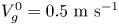 $V_g^0=0.5\ \textrm {m}\ \textrm {s}^{-1}$. For the experimental campaign detailed in this paper, the mean temperature of the test liquid was kept constant,
 $T_{mean}=25\,^{\circ }\textrm {C}$. The room temperature was about the same but with larger fluctuations,
 $T_{amb}=25\,^{\circ }\textrm {C} \pm 1.5\,^{\circ }\textrm {C}$.
2.1. Geometry
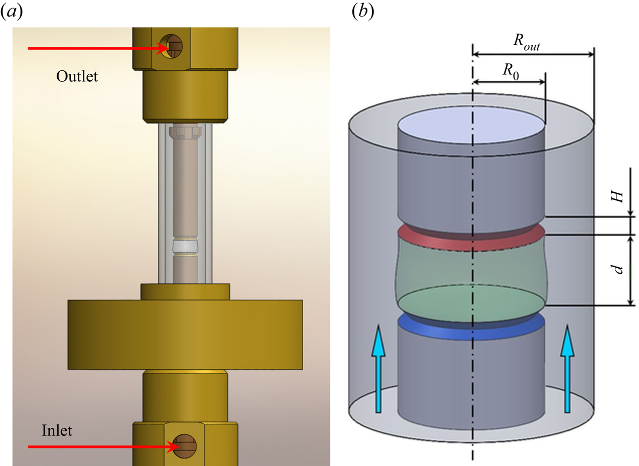
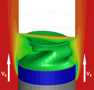
The heart of the experimental set-up consists of a LB surrounded by a long transparent tube as shown in figure 1(a) in scale. Note that the bottom rod has the same length as the upper one, but in the figure it is partially hidden by the heat exchanger. The more detailed schematic of the system, relevant to the experiment and numerical simulations, is shown in figure 1(b). The system consists of two co-axial cylinders. The outer cylinder is a glass tube of the radius  $R_{out}=5.0$ mm. The inner cylinder consists of two solid rods of the radius
 $R_0=3.0$ mm and a LB between them of the height
 $d=3.0$ mm, which is kept in its position by the surface tension force. The thickness of the heating/cooling parts of the rods is
 $h=1.0$ mm. The distance from the gas inlet to the cold disk is
 $H=25$ mm while
 $(H+h) /(R_{out}-R_0)=13$. The total length of the tube is
 $L=2H+2h+d$.
(a) Sketch of the central part of the set-up in scale (the inlet and outlet for gas are depicted). (b) Geometry and scales relevant to the experiment and numerical simulations. Gas enters from the cold side.

2.2. Temperature and gas flow management
There is no direct access to the liquid and all the sensors and feed pipes have to pass through the supporting rods. The working parts of the rods, which are in contact with the test liquid, are made of brass. Sharp edges are made in both rods to prevent the liquid from creeping over the edges of the rods. In this instrument only the tips of the rods (disk-shaped), which are in contact with liquids, are heated or cooled by the circulating heat-carrying liquid (a solution of water with ethylene-glycol). The temperature of the disks is adjusted independently. The temperature of the cold and hot disks was kept constant within  ${\pm }0.05\,^{\circ }\textrm {C}$. The external part of the rods is made of heat-insulating material and does not influence gas temperature.
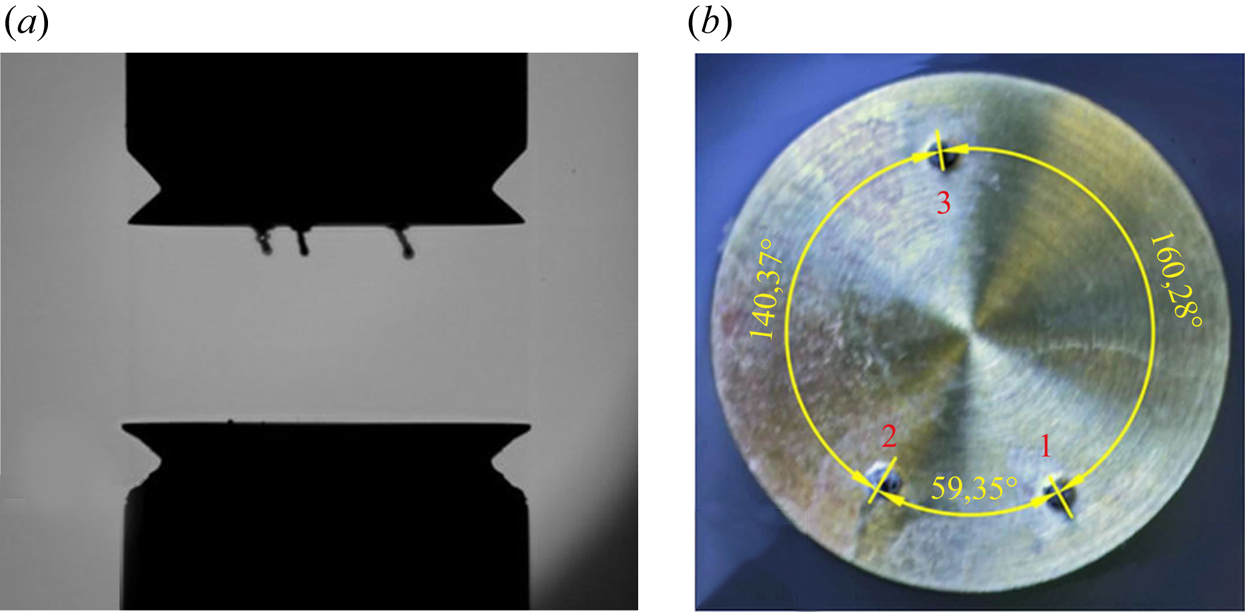
In the course of the experiment the temperature of the test liquid was recorded by three thermocouples and stored in a computer for further analysis. Embedded in the liquid from the upper rod were  $K$-type shielded thermocouples (with wires diameters of
 $24 \ \mathrm {\mu }\textrm {m}$), as shown in figure 2(a); their junctions are located at a distance of 0.3 mm from the surface. The thermocouples are not equally distant in the azimuthal direction and their angular positions are given in figure 2(b). They also have slightly different radial positions:
 $r_1=2.09$,
 $r_2=1.94$ and
 $r_3=2.12$ mm. The length of the thermocouples immersed into the liquid is 0.39 mm. In order to reduce noise on the thermocouples, the system with a high acquisition rate (National Instruments) was used ensuring a data logging frequency of 1 kHz at each channel.
(a) The thermocouples installed on the upper rod. (b) Geometrical configuration of thermocouples.

In the present study gas of a constant flow rate  $Q$ enters from the bottom through the annular duct of a size
 $(R_{out}-R_0)$. The mean velocity of the gas,
 $V_g^0,$ and its Reynolds number
 $Re_g$ were calculated from the measured flow rate
 $Q$ according to the relations
 \begin{equation} Q= {\rm \pi}(R^2_{out}-R^2_0)V_g^0, \quad Re_g=R_hV_g/\nu_g, \end{equation}
here  $R_h=2(R_{out}-R_0)$ is the hydraulic radius and
 $\nu _g$ is the gas kinematic viscosity. The gas flow rate
 $Q$ was set by means of a Bronkhorst mass flow regulator (EL-Flow) to ensure the required velocity. Gas was supplied to the cylindrical test section through a system of equally distributed channels to avoid turbulent flows and azimuthal motion of gas around the rod. The outlet of the test section was open to the atmosphere. Before entering the test section the gas was cooled/heated by passing through the heat exchanger regulated by a PID-controller PR59. The deviation of the velocity relative to its prescribed value was not greater than 0.1 %. The temperature of the gas was kept constant within
 ${\pm }0.02\,^{\circ }\textrm {C}$. Nitrogen (99.8 Vol%) was purchased in bottles from Air Liquide with nominal pressure 200 bar. Before entering the measuring system, the gas passed through a pressure regulator which decreased pressure down to
 $p=6$ bar at
 $T= 25\,^{\circ }\textrm {C}$.
2.3. Regulation of the LB volume
To establish a LB, the required volume of a liquid is injected through a small channel in the bottom rod using a syringe pump. The LB filled with  $n$-decane is slightly evaporating and the evaporation rate increases with the increase of gas velocity (Yasnou, Mialdun & Shevtsova Reference Yasnou, Mialdun and Shevtsova2012). The volume of the LB was controlled using an optical visualization of its shape. First, a given volume of liquid
 $\hat {V}_l$ is injected between the rods in the absence of a surrounding tube, and the readings of the syringe pump are compared with a calculated value using digital images of the interface shape
 $r=\tilde {h}(z)$ taken by the camera. Typically, they do agree within the volume control accuracy. The visible (synthetic) volume was calculated as
 \begin{equation} \hat{V}_l={\rm \pi} \int_0^d \tilde{h}^2(z)\,\textrm{d}z. \end{equation}
The procedure is then repeated for the LB with the tube installed. Due to the distortions by the tube, the optically measured volume  $V_l'$ does not coincide with that precisely measured by the syringe pump
 $\hat {V}_l$. The distorted value of
 $V_l'$ was entered as the reference into the control system. In the course of the experiments, the volume was calculated in real time using the images of the interface shape
 $r=\tilde {h}(z)$. The current value was compared with the reference and a command was sent to the syringe pump to inject a required volume of liquid. The computerized injection system allows maintaining the volume with a precision of 0.05 %. In all the experiments the relative liquid volume
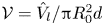 ${\mathcal {V}}= {\hat {V}_l}/{{\rm \pi} R_0^2d}$ was kept constant,
 ${\mathcal {V}}=1.0$. The physical properties of the fluids are given in table 1.
Physical properties of  $n$-decane and nitrogen at
 $25\,^\circ \textrm {C}$: the dynamic viscosity
 $\mu$, the thermal diffusivity
 $\chi ,$ the thermal conductivity
 $k$, the density
 $\rho$, the thermal expansion
 $\beta _T =-(1/\rho _0)\,\textrm {d}\rho /\textrm {d}T$, the Prandtl number
 $Pr= \nu /\chi .$ The other properties of
 $n$-decane used in this study are the surface tension
 $\sigma =23.83$ (
 $20\,^\circ \textrm {C})\ \textrm {mN}\ \textrm {m}^{-1}$ and the latent heat of evaporation
 $L_{lg}= 2.63\times 10^5\ \textrm {J}\ \textrm {kg}^{-1}$.

2.4. Experimental protocol and generation
Each experiment consisted of the following steps.
(a) A LB of a given volume (
 ${\mathcal {V}} =1.0$) was formed by injecting $n$-decane from the push syringe.
(b) A gas flow at the required temperature was activated immediately after filling the LB to avoid vapour condensation on the internal walls of the glass tube.
(c) Regulation of the LB volume was switched on.
(d) An initial temperature difference
${\rm \Delta} T=5\text {--}6\,^{\circ }\textrm {C}$, which is below the critical one, was applied between the supporting rods and waiting time was allowed for the stabilization of all the parameters of the system.(e) Records of all the thermocouples and thermistors were activated,
${\rm \Delta} T$ increased with ramping rate $0.045\,^{\circ }\textrm {C}/\textrm {min}$.





3. Mathematical model
3.1. Governing equations
The physical problem investigated is the same as in the experiment. The gas is assumed to be incompressible in consistency with the low pressure drop between the tube ends. The liquid and gas are considered as Newtonian fluids with temperature-dependent properties. The density  $\rho$ and the surface tension
 $\sigma$ are temperature-dependent quantities and they are expanded in Taylor series up to the first order,
 \begin{gather} \sigma = \sigma_0 -\gamma\left(T-T_0\right) + O(T-T_0)^2, \end{gather}
 \begin{gather}\rho = \rho_0 \left[1-\beta_T \left(T-T_0\right)\right] + O(T-T_0)^2, \end{gather}
where  $\gamma$ is the temperature coefficient of surface tension,
 $\beta _T$ is the thermal expansion coefficient and
 $T_0=T_{mean}=25\,^{\circ }\textrm {C}$. The reference quantities
 $\sigma _0$,
 $\rho _0$ and
 $\nu _0$ are evaluated at the mean temperature
 $T_0$.
The variation of the surface tension  $\gamma$ is essential, as it is one of the driving forces of the flow in a two-phase system and it appears in boundary conditions. The dynamics of the two-phase system in the geometry of figure 1(b) is described by the momentum, continuity and heat transfer equations for incompressible Newtonian fluids in the framework of the Boussinesq approximation:
 \begin{gather} \partial_t{\boldsymbol{V}} + ({\boldsymbol{V}} \boldsymbol{\cdot} \boldsymbol{\nabla}) {\boldsymbol{V}} = - \frac{1}{\rho}\boldsymbol{\nabla} P + \frac{\mu}{\rho} \nabla^2 {\boldsymbol{V}} + \boldsymbol{g}, \end{gather}
 \begin{gather}\boldsymbol{\nabla} \boldsymbol{\cdot} {\boldsymbol{V}} = 0, \end{gather}
 \begin{gather}\partial_t T + {\boldsymbol{V}} \boldsymbol{\cdot} \boldsymbol{\nabla} T = \chi \nabla^2 T. \end{gather}
Here  $\boldsymbol {V}$ and
 $p$ denote the velocity and pressure fields,
 $T$ is the temperature;
 $\mu$ is the dynamic viscosity;
 $\chi$ is the thermal diffusivity and
 $\boldsymbol {g}$ is the gravity vector. The superscripts ‘l’ (liquid) and ‘g’ (gas) are omitted in the above equations since they are identical for liquid and gas. However, they will be used in boundary conditions.
3.2. Boundary conditions
Below we discuss the boundary conditions of a two-phase flow system with an inlet and outlet. In the considered case of  $n$-decane the static Bond number is relatively small,
 $Bo_{st}=\rho g d^2/\sigma =2.7$, and the effect of static deformation will not be considered. As concerns dynamic deformation, the recent experimental studies by Matsunaga et al. (Reference Matsunaga, Mialdun, Nishino and Shevtsova2012) showed that in the geometry of interest in the isothermal case the interface deformation by a gas stream (
 $Re_g \leqslant 550$) is about a few microns. In the non-isothermal case experimental (Ferrera et al. Reference Ferrera, Montanero, Mialdun, Shevtsova and Cabezas2008; Montanero, Ferrera & Shevtsova Reference Montanero, Ferrera and Shevtsova2008) and numerical (Shevtsova et al. Reference Shevtsova, Mialdun, Ferrera, Ermakov, Cabezas and Montanero2008) studies reported that the interface deformation caused by a thermocapillary steady flow is proportional to the capillary number which is defined as
 \begin{equation} Ca_{Ma}=\sigma_T {\rm \Delta} T/\sigma. \end{equation}
It leads to the similar value of the interface deformation which is about  $15\text {--}25\ \mathrm {\mu } \textrm {m}$. So, for the parameters of interest, the interface deformation is slightly smaller than one-step size of the computational spatial grid.
(1) The boundary conditions on the free surface  $r=R_0$ between the liquid and gas are as follows.
(a) The balance of viscous and thermocapillary forces is
(3.7)where\begin{equation} \left[ P_l - P_g \right]{n}_i- \left( { S}_{ik}^l{ n}_k - { S}^g_{ik}{ n}_k\right)=\frac{\sigma }{\mathcal{R}} { n}_i - \frac{\partial\sigma}{\partial x_i}, \end{equation}${S}_{ik} = {S}= \eta (\partial V_i / \partial x_k + \partial V_k / \partial x_i )$ is the viscous stress tensor, ${\mathcal {R}}$ is the curvature, the normal vector $\boldsymbol {n}$ is directed out of the liquid. The tangential projections of (3.7) define the driving thermocapillary force in axial and azimuthal directions, $j=1,2$,
(3.8)\begin{equation} \boldsymbol{\tau}\boldsymbol{\cdot} {\boldsymbol{S}}^l\boldsymbol{\cdot}{\boldsymbol{n}} - \boldsymbol{\tau}\boldsymbol{\cdot} {\boldsymbol{S}}^g \boldsymbol{\cdot} {\boldsymbol{n}}= - \tau^{j}\boldsymbol{\cdot}\boldsymbol{\nabla}\sigma. \end{equation}(b) The tangential velocities of liquid and gas are equal; the temperatures of liquid and gas are equal:
(3.9a,b)\begin{equation} {\boldsymbol{V}}_{\tau}^l= {\boldsymbol{V}}_{\tau}^g, \quad T^l=T^g; \end{equation}(c) The kinematic condition at the non-deformable interface provides
(3.10)\begin{equation} V_r =0. \end{equation}(d) The liquid weakly evaporates on the interface. The energy conservation at the interface implies a balance between the heat fluxes in both phases and the heat of evaporation
(3.11)where\begin{equation} k^l \partial_{n}{T^l} = k^g \partial_{n}{T^g} - L_{lg}J, \end{equation}$L_{lg}$ is the latent heat of vapourization, $J$ is the mass flux of evaporated liquids through the interface given in table 1. The value of $J$ has been experimentally measured in this study, see § 4. The evaporation is not limited by the diffusion due to a gas stream which has swept vapour. The normal velocity caused by evaporation is small compared to the velocity of thermocapillary motion, and it can be neglected.




(2) On the lateral surfaces of the rods, which are in contact with gas, no-slip conditions are imposed:
 \begin{equation} \boldsymbol{V}^g(r=R_0)=0 \quad \mbox{when} \ 0 \leqslant z \leqslant (H+h); \quad H+2h+d \leqslant z \leqslant L. \end{equation}
The rods are thermally insulated except the small parts of the thickness  $h$ which are in contact with liquid:
 \begin{gather} \partial_n T =0 \quad \mbox{when} \ 0 \leqslant z \leqslant H; \quad H+2h+d \leqslant z \leqslant L; \end{gather}
 \begin{gather}T=T_0-{\rm \Delta} T/2 \quad \mbox{when} \ H \leqslant z \leqslant H+d; \end{gather}
 \begin{gather}T=T_0+{\rm \Delta} T/2 \quad \mbox{when} \ H+h+d \leqslant z \leqslant H+2h+d. \end{gather}
(3) The wall of the external tube is thermally insulated and no-slip conditions are imposed for velocity:
 \begin{equation} \partial_n T =0, \quad {\boldsymbol{V}^g}=0 \quad \mbox{when} \ r=R_{out}, \quad 0 \leqslant z \leqslant L.\end{equation}
(4) According to the experimental protocol, the required flow rate of the gas is imposed at the inlet,  $z=0$, where the flow is fully developed, unidirectional and only the axial velocity is non-zero. Then the inlet velocity distribution is related to the flow rate as (Gaponenko, Ryzhkov & Shevtsova Reference Gaponenko, Ryzhkov and Shevtsova2010)
 \begin{equation} V_g=\frac{2}{{\rm \pi} R_{out}^2}\frac{Q}{\left[k^4-1-\dfrac{(k^2-1)^2}{\ln k}\right]}\left[\left(\frac{r}{R_{out}}\right)^2-1-\frac{(k^2-1)}{\ln k}\ln \left(\frac{r}{R_{out}}\right)\right], \end{equation}
where 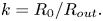 $k=R_{0}/R_{out}.$ The temperature of the gas is a parameter of the problem
 \begin{equation} T^g = T_{in}, \quad \mbox{when} \ z=0, \quad R_{0} < r < R_{out} \end{equation}
(5) At the outlet we assume that perturbations do not penetrate back inside the tube as it was discussed previously by Gaponenko et al. (Reference Gaponenko, Ryzhkov and Shevtsova2010), correspondingly, all the derivatives in the direction of the flow are equal to zero:
 \begin{equation} \frac{\partial {\boldsymbol{V}}}{\partial z} = 0, \quad \frac{\partial T^g}{\partial z} =0. \end{equation}
As an initial state, zero velocity field and mean temperature have been chosen.
The major parameters controlling the flow are Prandtl number  $Pr$, Grashof number
 $Gr$, Marangoni number
 $Ma$, viscosity ratio
 $\tilde \mu$, thermal conductivity ratio
 $\tilde {k}$:
 \begin{equation} Pr=\frac{\mu}{\rho \chi}, \quad Gr=\frac{\beta_T {\rm \Delta} T g d^3}{\nu^2},\quad Ma=\frac{\gamma {\rm \Delta} T d }{\mu^l \chi^l},\quad \tilde{\mu}=\frac{\mu^l}{\mu^g}, \quad \tilde{k}=\frac{k^l}{k^g}. \end{equation}
In addition, the control parameters for the LB geometry are the relative liquid volume  ${\mathcal {V}},$ and two aspect ratios:
 \begin{equation} {\mathcal{V}}= \frac{\hat{V}_l}{{\rm \pi} R_0^2d}, \quad \varGamma=\frac{d}{R_0}, \quad \varGamma_R=\frac{R_{out}}{R_0}. \end{equation}
For the experimental geometry and fluid properties listed in § 2.1, the dimensionless parameters can be written in the way convenient for comparison with literature data ( $V_g^0$ is in
 $\textrm {m}\ \textrm {s}^{-1}$):
 \begin{gather} Gr^g=3.63\times 10^{3} {\rm \Delta} T, \quad Gr^l=2.06\times 10^{5} {\rm \Delta} T, \quad Ma=4.95\times 10^{3} {\rm \Delta} T, \end{gather}
 \begin{gather}Re^g=2.54\times 10^{2} V_0^g, \quad \tilde{\mu}=42.13,\quad \tilde{k}=5.19, \quad {\mathcal{V}}=1, \quad \varGamma=1, \quad \varGamma_R=1.67. \end{gather}
3.3. Numerical method and validation
The commercial solver ANSYS Fluent 17.2 was used for solving governing equations (3.3)–(3.19a,b). The problem was solved using dimensional variables  $(x, y, z)$ in two domains for each phase separately with taking into account the boundary conditions at the interface. In order to satisfy the conditions at the interface very accurately, an iterative procedure developed for a two-dimensional problem (Shevtsova et al. Reference Shevtsova, Gaponenko and Nepomnyashchy2013) was used.
Time dependence is treated using a standard implementation of the pressure-implicit with splitting of operators pressure-velocity coupling scheme, while spatial discretization is done using the pressure staggering options technique for the pressure equation. This procedure is similar to the staggered-grid schemes used with structured meshes. A third-order monotone upstream-centered scheme for conservation laws technique is used for the momentum and energy equations. The reliability of the calculations was checked by halving the time step used in the calculations presented here (0.001 s) to verify if there is any influence on the flow organization. The check indicated negligible changes.
Computations in multi-domains require a complicated computational mesh, which was generated by the commercial code GAMBIT. A non-uniform grid was chosen for a space discretization as follows. In the liquid domain  $N_z = 60$ with stretch factor 0.973 near cold and hot corners. In the radial direction,
 $N_r=40$, the denser mesh was near the interface with stretch factor 0.97 and a more rare mesh was near the axis with stretch factor 1.03. In the gas domain the mesh is divided into five parts: the interfacial part, two parts of the length
 $h$ adjacent to the hot and cold disks and two parts of the length
 $H$ adjacent to the rods. The cells number for the interfacial part of the gas phase is the same as for the liquid phase. For the part of the hot (cold) disks,
 $N_z = 20$ with stretch factor 0.97 (towards liquid) and 1.05 (towards the thermally insulated part). For the thermally insulated part adjacent to the rods,
 $N_z = 25$ with stretch factor 1.03. In the radial direction
 $N_r = 25$ with stretch factor
 $0.9$ for all the parts of the gas phase. In the azimuthal direction
 $N_{\varphi } = 40$ for all the mesh parts. The smallest cells lie in the region of the liquid–gas interface where the mesh cell size is equal to
 $h_{min}=3.30912^{-5}$ m. The thickness of the boundary layer
 $\delta$ for Marangoni flows is scaled as (Kuhlmann & Rath Reference Kuhlmann and Rath1993)
 \begin{equation} \delta\sim (d/R) (Ma/Pr)^{-1/3} \approx 0.046-0.066 \quad (\textrm{depending}\ \textrm{on}\ {\rm \Delta} T). \end{equation}
The dimensionless mesh size near the interface  $h_{min}/R_0\approx 0.011;$ thus, there are 4–6 points inside the boundary layer. Near the corners, a regularization of boundary conditions developed by Wanschura et al. (Reference Wanschura, Shevtsova, Kuhlmann and Rath1995) is used on 5 % of the interface length. The convergence of the numerical solutions for different meshes was examined in the two-dimensional case (Shevtsova et al. Reference Shevtsova, Gaponenko and Nepomnyashchy2013). We expect this approach to be a good compromise between computational cost and numerical accuracy.
To ensure that the three-dimensional model provides physically meaningful results, further validation work has been undertaken by comparison with recently published results of LSA by the research group of Kuhlmann (in Shevtsova et al. Reference Shevtsova, Gaponenko, Kuhlmann, Lappa, Lukasser, Matsumoto, Mialdun, Montanero, Nishino and Ueno2014). They used 5cSt silicone oil and argon as the test fluids. Our calculations for the same set of parameters ( $Pr=68$,
 $\varGamma =1$,
 $\varGamma _R=2$,
 $U_g=0$) provided
 $\widetilde {Re}_{cr}=Ma/Pr=620$ while the LSA result is
 $Re_{cr}=600$. The results differ only by about 3–4 % and the azimuthal wavenumber
 $m$ is identical,
 $m=1$. In the case of a gas flow, we compared our results with those of the same paper for
 $\widetilde {Re}=640$ for two opposite directions of gas moving with the velocity
 $V_g = \pm 0.5\ \textrm {m}\ \textrm {s}^{-1}$. Simulations revealed a TW with
 $m = 1$ in the case of positive velocity and a stable solution for negative velocity, which is fully consistent with the previous findings. We believe that the numerical model captures the essential features of the HTW properties, which are the dominant phenomena over the considered parameter range.
4. Evaporation of $n$-decane

Normal decane (chemical formula C10H22) is a weakly evaporating fluid. As discussed in § 2.3, the volume of the LB was kept constant in the experiments, and for this, a computer-controlled amount of fluid was continuously injected. The loss of fluid is associated with evaporation. Thus, the design of the set-up allows us to estimate the change in the liquid volume  ${\rm \Delta} \hat {V}_l$ at a given time interval
 ${\rm \Delta} t$ and, therefore, determine the evaporation rate. The global evaporation mass flux
 $J_g$ from a liquid surface of cross-sectional area
 $S$ can be defined as
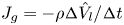 $J_g=-\rho {{\rm \Delta} \hat {V}_l}/{{\rm \Delta} t}$ and the evaporation rate per unit time and area is
 \begin{equation} J=-\frac{\rho}{S} \,\frac{{\rm \Delta} \hat{V}_l}{{\rm \Delta} t}. \end{equation}
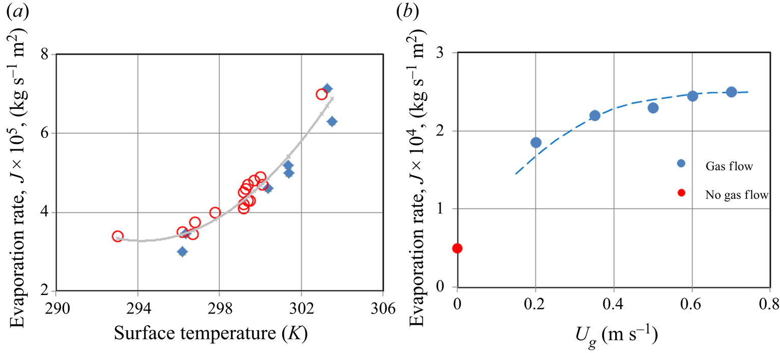
In order to determine the evaporation rate, the first tests were conducted without a forced gas flow along the interface. In this case the mechanism of evaporation can be attributed to diffusion and buoyancy-induced convection of vapour. The measurements were carried out in two experimental campaigns. In the first campaign the temperature of the cold rod was kept constant, and the tests were conducted at different temperatures of the upper rod, that is, at different  ${\rm \Delta} T.$ The results of this campaign are shown in figure 3(a) by the blue diamonds. The temperature of the interface was evaluated using common approximation for LBs as
 $T_s \approx T_{cold}+0.7 {\rm \Delta} T.$ In the second campaign the temperature of both rods was kept the same (
 $T_{cold}= T_{hot}=T_{mean}, {\rm \Delta} T=0$) and the experiments were carried out at different mean temperatures. These results are shown by the red circles. All the data was fitted by the second-order polynomial shown also in figure 3(a) by the grey curve. This curve corresponds to the expression (
 $T_s$ is measured in Kelvin)
 \begin{equation} J_{V_g=0}=(4.154\times 10^{-5}\cdot T_s^2 - 2.444 \times 10^{-2} \cdot T_s +3.598)\times 10^{-2} . \end{equation}
Average evaporation rate of  $n$-decane. (a) Dependence of the evaporation rate on the interface temperature when
 $V_g=0$. The cycles correspond to the experiments at
 ${\rm \Delta} T=0$ when
 $T_{mean}$ varies while the diamonds indicate experiments at different
 ${\rm \Delta} T$ when
 $T_{cold}$ was constant; the curve corresponds to (4.2). (b) Dependence of the evaporation rate on the gas velocity when
 $T_{mean}=298$ K,
 ${\rm \Delta} T=0.$ Note that the scales for
 $J$ in panels (a,b) are different.

In the series of the following experiments, the volume of the evaporated fluid was measured at several gas velocities while  $T_{mean}=25\,^{\circ }\textrm {C}$,
 ${\rm \Delta} T=0.$ As follows from figure 3(b), there is a large difference between the evaporation rate with and without the forced gas stream. However, the progressive increase of the gas velocity by four times (from
 $0.2\ \textrm {m}\ \textrm {s}^{-1}$ till
 $0.8\ \textrm {m}\ \textrm {s}^{-1}$) does not change drastically the evaporation rate. All the evaporated gas near the interface is swept away by a forced gas flow, and a purely convective mechanism can be considered; diffusion of the vapour in the gas does not play a role. Note that the liquid/gas viscosity ratio is large,
 $\mu _l/\mu _g\sim 50,$ and the effect of shear stress is insignificant for the considered velocities. The temperature of the interface was settled to be uniform, and the increase of the gas velocity saturates. Of course, the strong evaporation can lead to non-uniformity of the interface temperature and convection in liquid will play a role. This does not apply to
 $n$-decane in the temperature range under consideration. For the numerical simulations, we use (4.2) multiplied by the constant coefficient corresponding to the increase of the evaporation rate at a given gas velocity.
5. Flow visualization
5.1. Experimental
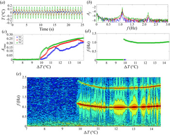
In the experiments, the temperature time series near the top disk of the LB were recorded by three thermocouples with a sampling rate of 20 Hz. Since the applied temperature difference was continuously increased with the ramping rate 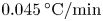 $0.045\,^{\circ }\textrm {C}/\textrm {min}$, the mean temperature of the thermocouples tips varied over time. In order to follow the evolution of an oscillatory instability, the deviation of temperature oscillations from temporal mean value was monitored. An example of thermocouple (TC) readings is shown in figure 4(a) in the case of the gas temperature
 $T_g=20.0\,^\circ \textrm {C}$ moving with velocity
 $V_g=0.5\ \textrm {m}\ \textrm {s}^{-1}$. The time series data was accumulated during a waiting period of at least one thermal time defined as
 $\tau _{th}= d^2/\chi = 107\ \textrm {s}$. Then the fast Fourier transform (FFT) was performed to characterize the oscillatory signals. The frequency spectrum was obtained for each data set consisting of 2048 points overlapping by 30 %. The typical results of FFT are shown in figure 4(b).
Flow characteristics procured from thermocouple readings;  $T_g=20.0\,^\circ \textrm {C}$ and
 $V_g=0.5\ \textrm {m}\ \textrm {s}^{-1}$. (a) Amplitude of temperature oscillations at
 ${\rm \Delta} T=10\,^\circ \textrm {C}$, (b) its power spectral density, (c) evolution of the oscillation amplitude with
 ${\rm \Delta} T$ near threshold, (d) evolution of the dominant frequency with
 ${\rm \Delta} T$ near threshold and (e) Fourier map.

The amplitude of the temperature oscillations over a much longer period ( ${\sim }1400$ s) is shown in figure 4(c) in terms of
 ${\rm \Delta} T$. Notably different amplitudes in various thermocouples indicate complex three-dimensional behaviour of the system. Having some experience, we can assume that the arrangement of the maxima and minima in figure 4(a) corresponds to a SW. Determining the Fourier spectra for each
 ${\rm \Delta} T$ enables the possibility to trace a continuous evolution of the frequency with time or
 ${\rm \Delta} T$; it is shown in figure 4(c,d) for the dominant frequency and the amplitude over the same range of parameters.
To gain further understanding, all the frequencies from the FFT are combined with their amplitude in order to build a Fourier map. The example of such a map is shown in figure 4(e). A Fourier map is an extended version of the panel (d), in addition to the dominant frequency, all harmonics are drawn, and their amplitudes are given by colours. The Fourier map allows us to conveniently track the evolution of flow states with the increase in the driving force, which is  ${\rm \Delta} T$. These maps are built independently for all three thermocouples. To conclude, the readings from three non-equidistant thermocouples provide the possibility to determine critical parameters such as
 ${\rm \Delta} T_{cr}$ and
 $f_{cr}$ and build the Fourier map. It may also give a hint about the wave type, although this needs to be checked.
5.2. Numerical
All the fields are regularly recorded during the simulations. The time evolution of temperature and velocity are monitored in the liquid at four azimuthally equidistant points in a plane at mid-height and at the same radial position close to the interface,  $r=2.5$ mm. Hereafter, we refer to these points as numerical thermocouples. The positions of these numerical thermocouples are shown in figure 5(c,d). In addition, three numerical thermocouples are placed at the same positions as the experimental ones. The development of the instability is investigated by means of FFTs performed on the temperature record of one of the thermocouples at mid-height of the LB. In all cases, the FFT is performed using the same number of points in the time series, i.e. 8192 (
 $2^{13}$), which covers a period of time of about 50 s. This allows for a comparison of the FFT amplitude
 $A_f$ for different cases. To reveal the direction of the HTW propagation and its azimuthal mode, three-dimensional temperature images were constructed for all the calculated cases. Some examples can be seen later in figures 9 and 14.
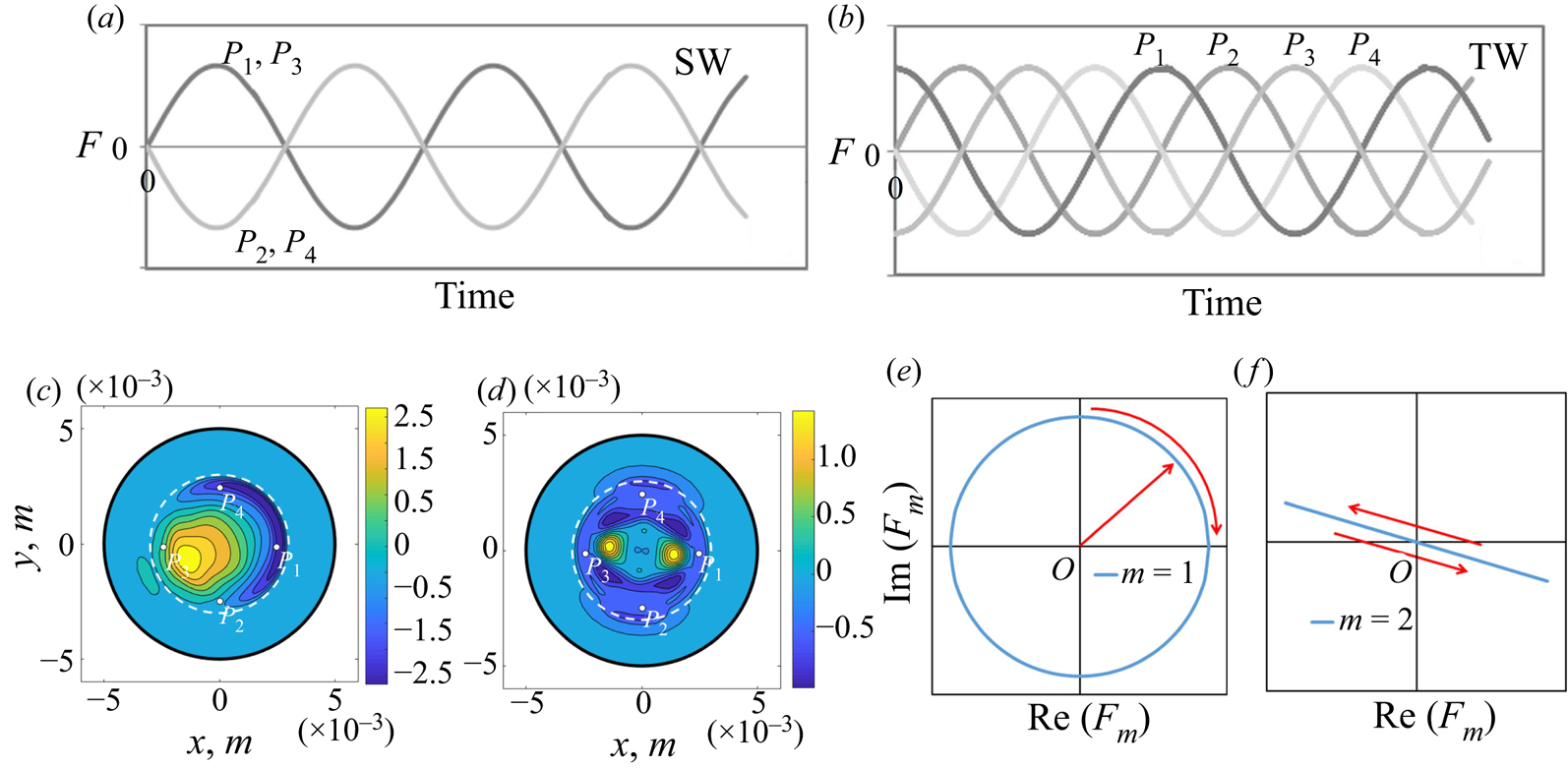
Flow visualization. The temperature signals on four azimuthally equidistant points  $P_i$ in the case of (a) SWs and (b) TWs. (c,d) Snapshots of the temperature field perturbations in the cross-section at mid-height of the LB. Two different types of symmetry of the solutions (c)
 $m=1$ and (d)
 $m=2$. The white dashed line depicts the liquid–gas interface and
 $P_i$ indicates the location of numerical thermocouples. (e,f) Sketch of the trajectories of the dynamic system in the case of (e) TWs and (f) SWs.

5.3. Spatiotemporal evolution of HTWs
The instability leads to the development of a time-periodic three-dimensional flow  ${\tilde {F}}$, which can be represented at leading order as
 ${\tilde {F}}-F_0\approx {F}$, where
 $F_0$ is the undisturbed stationary flow. The HTWs, which develop following an oscillatory instability of a steady axisymmetric flow, are characterized by integer values of the azimuthal wavenumber
 $m$. Because of the periodicity of the problem in the azimuthal direction, the spectrum of azimuthal wavenumbers is discrete. Due to the symmetry
 $\varphi \to -\varphi$, in the case of a critical wavenumber
 $m\neq 0$, the linear stability theory predicts the existence of two critical disturbances corresponding to waves moving in opposite directions,
 \begin{gather} F_+={\hat{f}}_+(r,z)\exp(\textrm{i}m\phi+\omega_0 t)+\textrm{c.c.}, \end{gather}
 \begin{gather}F_-={\hat{f}}_-(r,z)\exp(\textrm{i}m\phi-\omega_0 t)+\textrm{c.c.} \end{gather}
At threshold, the solution  ${F}$ of the linearized stability problem can be written as the sum of both disturbances with arbitrary coefficients
 $a_+$ and
 $a_-$, i.e.
 \begin{equation} {F}=a_+F_+ + a_-F_-. \end{equation}
Typically, one observes either  $a_- = a_+$ (a SW), or that one of the amplitudes
 $a_{\pm }$ vanishes (a TW). A schematic representation, in the ideal case, of the time series for a SW and TW is shown in figure 5(a,b). For the SW (figure 5a), signals coincide for points that are separated by an azimuthal angle
 ${\rm \pi}$ (i.e.
 $P_1$ and
 $P_3$, or
 $P_2$ and
 $P_4$) while, for the TW (figure 5b), the signals at points
 $P_i$ are shifted by
 ${\rm \pi} /2$. Close to onset, the nonlinear dynamics is determined mainly by the interaction of the primary (lowest threshold) modes and, for a LB with aspect ratio
 $\varGamma =1$, these are the ones with wavenumbers
 $m=1$ and
 $m=2$. The typical structure of the temperature disturbances in the cross-section of a LB for this type of wave is illustrated in figure 5(c,d), where one pair of hot and cold spots corresponds to
 $m=1$ and two pairs of spots correspond to
 $m=2$. Using temperature signals at points
 $P_i$ one can, in some cases (Lappa Reference Lappa2010), discern if the wave is a SW or TW, and even its wavenumber, by considering dependencies (attractors),
 $T(P_i )$ versus
 $T(P_j )$; here the subscripts
 $i$,
 $j$ indicate the TC numbers from figure 5.
In the supercritical region, the time-periodic solution has the form
 \begin{equation} F=\sum_{m=-\infty}^{\infty}\sum_{n=-\infty}^{\infty}\hat{f}_{m,n}(r,z) \exp(\textrm{i}m\phi+\textrm{i}n\omega t), \end{equation}
where 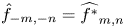 $\hat {f}_{-m,-n}=\widehat {f^*}_{m,n}$,
 $m$ is the wavenumber and
 $n$ is the number of the combinational Fourier harmonic for that component with wavenumber
 $m$.
In the following we are interested in the azimuthal wavenumber and such properties whether the wave is travelling or standing. To do this, we rewrite (5.4) in a more compact form:
 \begin{equation} F= \sum_{-\infty}^{\infty}{\tilde{f}_m}(r,z,t)\exp(\textrm{i}m\varphi). \end{equation}
To examine the properties of a HTW  $F_m$ with a given azimuthal number
 $m$, the perturbation quantity
 ${\tilde {f}}$ is decomposed into real and imaginary parts at a fixed horizontal position
 $z=z^*$,
 \begin{align} F_m(z^*,t)&= \int_0^{R_0}\int_0^{2{\rm \pi}}{\tilde f}(r,z^*,t)\,\textrm{e}^{-\textrm{i}m\varphi}r\, \textrm{d}r\,\textrm{d}\phi\nonumber\\ & =\int {\tilde{f}}(r,t)\cos(m\varphi) r \,\textrm{d}r \,\textrm{d}\varphi - \textrm{i}\int {\tilde{f}}(r,t) \sin(m\varphi) r \,\textrm{d}r \,\textrm{d}\varphi\nonumber\\ & =\textrm{Re}[F_m(t)] - \textrm{i}\,\textrm{Im}[F_m(t)], \end{align}
where  ${\tilde {f}}$ can be any of
 $({\boldsymbol {V}}, P, T).$ Comparison with experiment is an essential part of the study and, since temperature is a directly measured experimental quantity,
 $\tilde {f}$ is associated with the temperature of the liquid. The perturbation
 $\tilde {f}$ can be determined from the computed quantity
 $\tilde {F}(r,\varphi , z)$ as
 \begin{equation} {\tilde{f}}(r,\varphi, z)=\tilde{F}(r,\varphi, z) - 1/2{\rm \pi} \int_0^{2{\rm \pi}} \tilde{F}(r,\varphi, z) \,\textrm{d}\phi.\end{equation}
In practice, in numerical modelling, we subtracted the steady-state solution obtained on the same mesh. The evolution in time of the real and imaginary parts,  $\textrm {Re}[F_m(t)]$ and
 $\textrm {Im}[F_m(t)]$, is shown for the TW
 $m = 1$ in figure 5(e), which appears in the supercritical regime with
 ${\rm \Delta} T=10\,^{\circ }\textrm {C}$ and
 $T_g=22.5\,^{\circ }\textrm {C}$. The observation of the displacement of the temperature field with time (i.e. the position of a point on a trajectory) is made with respect to the two-dimensional steady state; the origin ‘
 $O$’ is where
 $\textrm {Re}[F_m(t)]=\textrm {Im}[F_m(t)]=0$. In the case of a TW, the trajectory during one period of oscillation traces a circle with a centre at the point ‘
 $O$’. In the case of a SW, the trajectory appears as a straight line crossing through the centre, as shown in figure 5(f).
To further investigate the relationship between the azimuthal mode and frequency in some cases, we perform an additional Fourier transform of the periodic functions  $\textrm {Im}[F_m(t)]$ and
 $\textrm {Re}[F_m(t)]$. Since this analysis of both functions gives identical results for frequency but with different amplitudes, we may consider only the real part,
 $\textrm {Re}[F_m(t)]$. This procedure connects the wave with mode
 $m$ to the set of frequencies
 $\omega _n$. The amplitude of the mode
 $m$ with frequency
 $n$ obtained as a result of the Fourier transform of the periodic function
 $\textrm {Re}[F_m(t)]$ is denoted as
 $a_{m,n}$. This procedure allows us to describe a HTW at a specified point in the form of (5.4). To clarify the processing procedure described above, it is illustrated graphically in table 2.
Scheme for the processing of results using three routes. Route r1: A visual inspection (V.I.) of time-dependent signals (as in figure 5a,b) is performed in order to discern the wave type (SW or TW) and the wavenumber  $m$. This route also includes three-dimensional (3D) views of all fields (as in figures 5, 9, 14, and in the movies developed). Route r2: This provides complete frequency characteristics and enables the construction of Fourier maps as in figure 4; it is similar for both experiments and simulations. Route r3: This provides definite information about the HTW (SW or TW, and
 $m$) and determines the amplitudes of
 $\textrm {Re}[F_m(t)]$ and
 $\textrm {Im}[F_m(t)]$, which gives information about the dominant and secondary HTW modes and assigns one of the frequencies determined on route r2 to each wave.

In the experiments there are only three thermocouples available. It is a challenging task to determine the dynamics of the system using temperature records from these three unequally spaced thermocouples. In this case, (5.6) cannot be used in the given form since only three of the coefficients are linearly independent. Nonetheless, since the azimuthal locations  $\varphi _n$ of the thermocouples are known precisely, we may use the following approach:
 \begin{align} F_{m}(t)&= \sum_{j=1}^{3}{\tilde f}_j(t)\cos(m\varphi_j) -\textrm{i} \sum_{j=1}^{3}{\tilde f}_j(t)\sin (m\varphi_j) \nonumber\\ &= \textrm{Re}(F_m(t)) - \textrm{i}\,\textrm{Im} (F_m(t)) . \end{align}
As an output, we do not calculate the true Fourier harmonics and, instead of the circle or straight line shown in figure 5(d), distorted versions can appear. To apply this approach to the experiments, readings from the thermocouples were individually treated, i.e. the mean temperature was calculated separately for each thermocouple. The thermocouples, while having a short response time, are never noise free and this noise may further complicate the interpretation of trajectories. Complementary efforts that combine coordinated experiments and numerical simulations are helpful in understanding the nonlinear dynamics of the flow.
6. Results
6.1. Global picture of oscillatory states
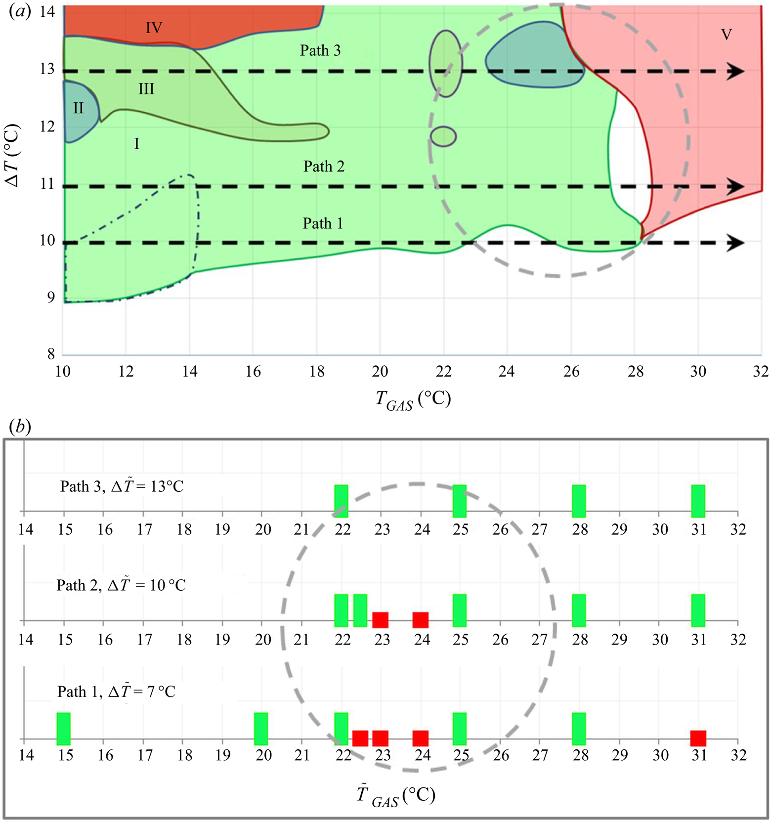
In the experiments the progress of instability was investigated by means of Fourier maps at given gas temperatures, which are built in terms of a frequency versus the applied temperature difference between the rods (see figure 4e). Availability of numerous Fourier maps allows creating one global view of the oscillatory states as shown in figure 6(a). The coloured region corresponds to oscillatory instability, while the white area indicates a steady flow. The first impression from this global picture is that the threshold of instability only weakly depends on the gas temperature; critical  ${\rm \Delta} T$ demonstrates a continuous slight increase until
 $T_g\leqslant 20\,^{\circ }\textrm {C}$. Cooling by gas provides a stabilizing effect. A further increase in the gas temperature displays local rises and falls of
 ${\rm \Delta} T_{cr},$ which can be explained by the interaction of the heat flux and shear stress. While the effect of shear stress formally can be neglected in the limit of a large viscosity ratio, it does play a role at small values of heat transfer through the interface. When both are weak, the interplay of heat transfer with shear rate leads to small changes in the critical curve. The averaged heat flux at the threshold decreases with
 $T_g$ and even changes sign at
 $T_g\sim 30\,^{\circ }\textrm {C}$ (Yasnou et al. Reference Yasnou, Gaponenko, Mialdun and Shevtsova2018). This emphasizes the extreme sensitivity of the flow dynamics to the interfacial boundary conditions. The observed trends in the behaviour of the critical curve suggest that at a certain
 ${\rm \Delta} T$ oscillatory instability can be suppressed or promoted by changing the gas temperature.
Summary of experimental and numerical tests in a LB ( $Pr=14$) subjected to a parallel gas stream when
 $U_g = 0.5\ \textrm {m}\ \textrm {s}^{-1}$,
 $Pr_g=0.7$. Three paths are selected for a detailed analysis. A similar intriguing evolution of the flow states in experiments and simulations was observed in the parameter space (
 ${\rm \Delta} T, T_g$), which is highlighted by grey circles. (a) The global view of dynamic regimes obtained experimentally. The coloured region corresponds to oscillatory instability, while the non-coloured area indicates a steady flow. Different colours correspond to various periodic states: (I) periodic; (II) quasi-periodic with two frequencies; (III) quasi-periodic with three frequencies; (IV) noisy quasi-periodic with three frequencies; (V) periodic. (b) Map of numerical results. The green bars correspond to oscillatory states while the red bars indicate the stationary states.

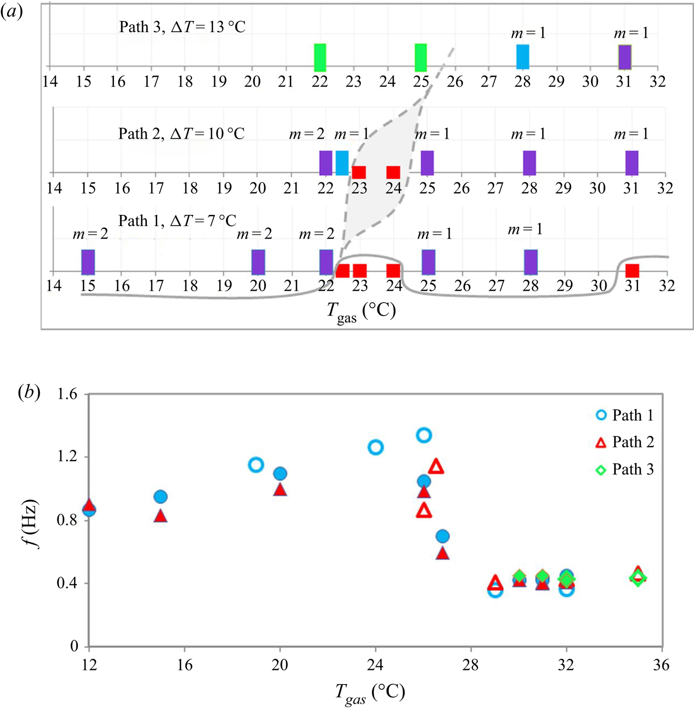
Above the threshold, the flow dynamics can be divided in several regimes with respect to the number of dominating modes and frequencies. The location of particular regimes are outlined by different colours in figure 6. However, the most intriguing behaviour of the oscillatory flow is observed at gas temperatures above the mean value but below the temperature of the hot rod, i.e.  $26\,^{\circ }\textrm {C} < T_g < 30\,^{\circ }\textrm {C}$. Within this range of
 $T_g$, hydrothermal instability completely disappears and then sets again, forming a stability window. In the following, attention will be focused on this area (outlined by the grey circle), and the evolution of hydrothermal instability will be traced along the three paths according to given
 ${\rm \Delta} T$: (i) path I passing below the stability window,
 ${\rm \Delta} T=10\,^{\circ }\textrm {C}$; (ii) path II crossing the stability window,
 ${\rm \Delta} T=11\,^{\circ }\textrm {C}$; (iii) path III passing above the stability window,
 ${\rm \Delta} T=13\,^{\circ }\textrm {C}$.
For the complete analysis of the problem, our experiments are supplemented by three-dimensional numerical simulations in the framework of a two-phase model. The state points, at which the calculations were performed along the paths selected above, are marked by bars in figure 6(b). The map of numerical results displays alteration between oscillatory and stationary states, providing an analogy with the experimental findings.
We do not expect absolute quantitative agreement because experimental procedure contains many distinct points which are not taken into account in simulations: continuous ramping although small, the deformation of the LB by gravity, possible contamination of the interface over time, etc. Nevertheless, it is clear that the grey circle on the numerical map outlines the flow states which replicate the experimental ones. Thus, the goal of numerical simulation is to find better interpretation of the experimental observations from the view point of nonlinear dynamics. On the quantitative side, there is a small shift in  ${\rm \Delta} T$ and in gas temperature by about
 $3\text {--}4\,^{\circ }\textrm {C}$. To avoid confusion, hereafter, the temperature used in the numerical simulations is denoted by a slightly different letter,
 $\tilde {T},$ and, when comparing, one should keep in mind that
 $\tilde {T}_g \sim T_g-3\text {--}4\,^{\circ }\textrm {C}$. Primarily, our study below will focus on the encircled regions in figure 6.
In all the simulations, first, a steady state was calculated, and it was used as initial conditions for time-dependent simulations on the same grid without adding noise. The calculations lasted longer than one thermal time,  $\tau _{th}=107$ s, and were stopped when
 $T$ and
 $\boldsymbol {V}$ oscillations became self-sustained. Our numerical model includes evaporation. Locally, the heat flux due to evaporation could reach 10 % of the total heat flux, but was never the dominant heat transfer mechanism.
6.2. Path 1
(Experiment, path 1.) Path 1 at  ${\rm \Delta} T=10\,^{\circ }\textrm {C}$ traverses the global map in terms of (
 ${\rm \Delta} T,T_g$) very close to the instability threshold, especially at the gas temperatures higher than the temperature of the cold wall, as seen in figure 6. As the gas temperature rises above
 $T_g \sim 22\,^{\circ }\textrm {C}$ along this path, the oscillatory flow passes several cycles of stabilization and destabilization. In order to understand the HTW properties at the onset of instability, we consider the dynamics of a point that is very close to the threshold, i.e.
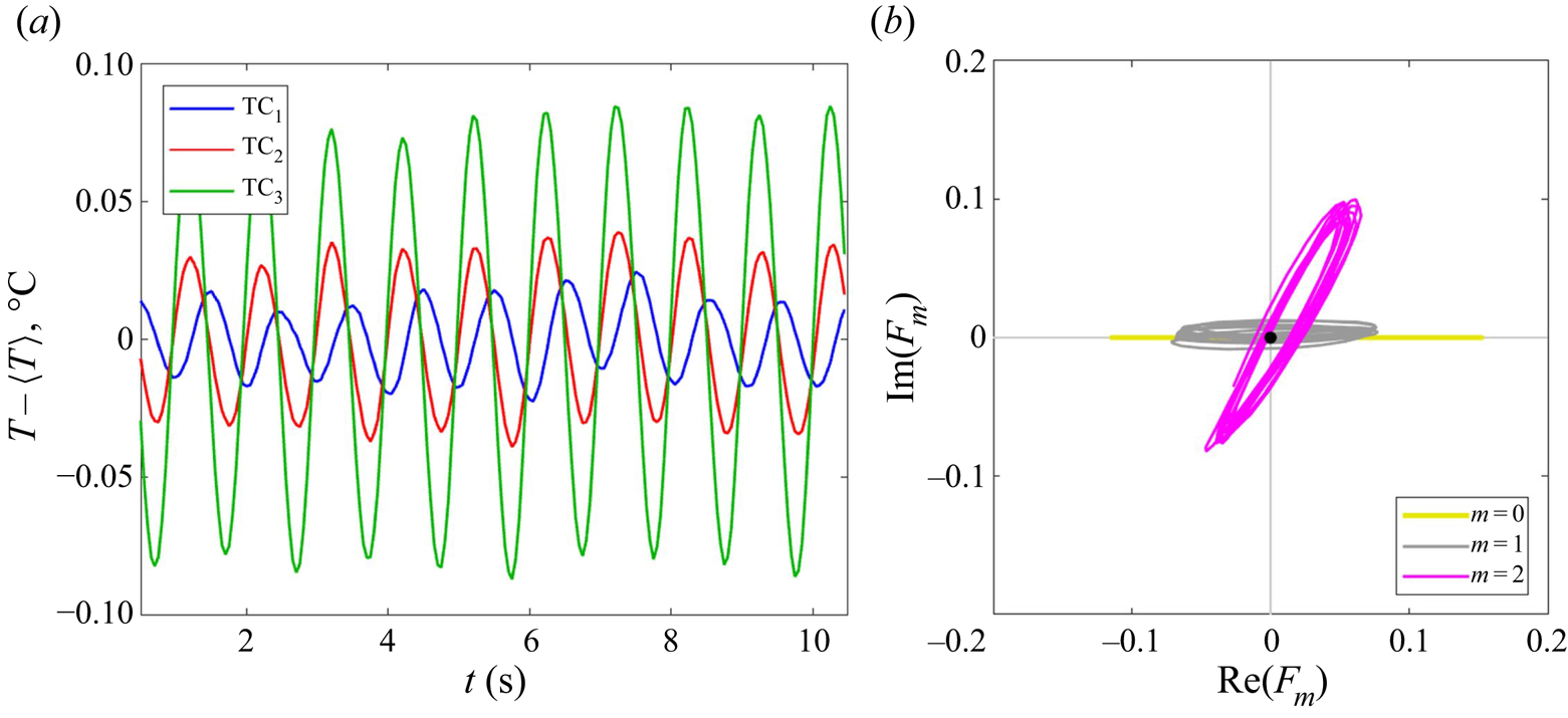
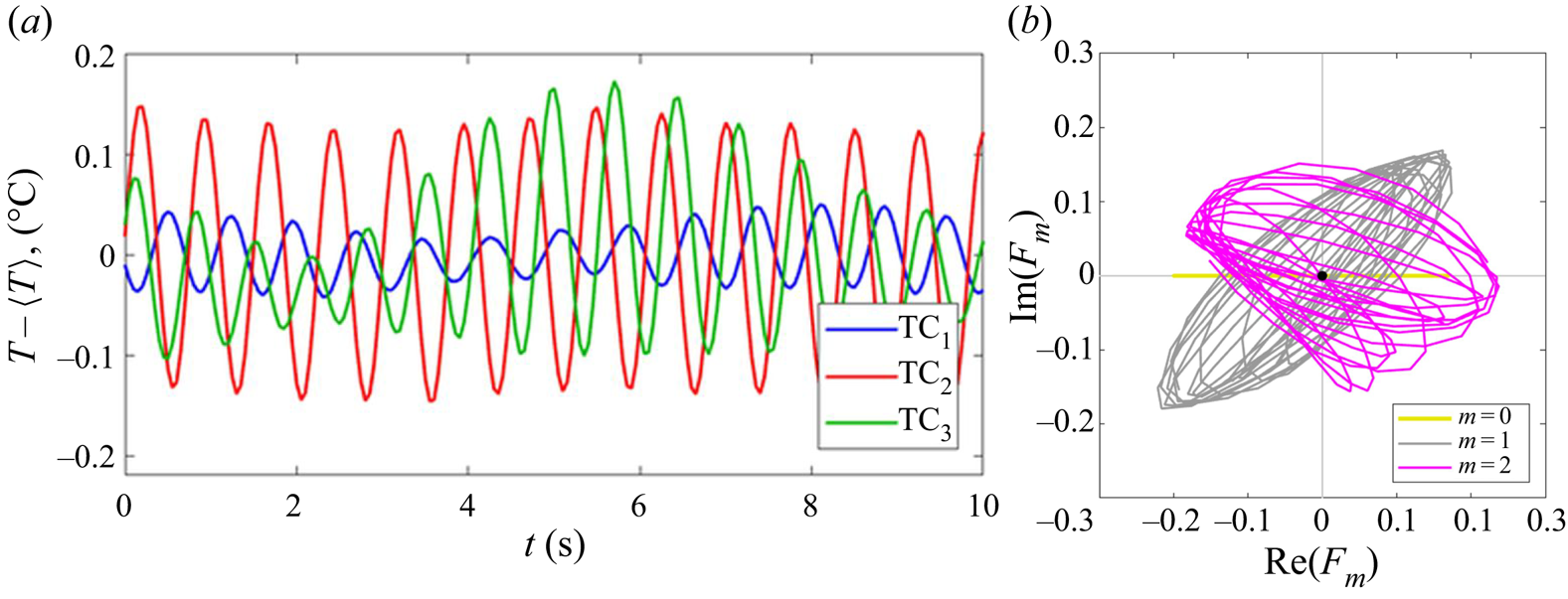
 $T_g=26\,^{\circ }\textrm {C}$. The temperature signals from three non-equidistant thermocouples are shown in figure 7(a). It can be noted that over the 10 oscillation periods presented, the mutual position of the maxima does not change with time. Given that the signals from two thermocouples, separated by
 ${\sim }0.8 {\rm \pi}$, have coinciding extrema, this gives a hint about the SW (see figure 5a for the reference).
(Path 1, experimental results.) (a) Temperature time dependence on three non-equidistant thermocouples. (b) Trajectories of the system in a phase plane. Here  ${\rm \Delta} T=10\,^{\circ }\textrm {C}$,
 $T_g=26\,^{\circ }\textrm {C}$,
 $V_g = 0.5\ \textrm {m}\ \textrm {s}^{-1}$ and
 ${\mathcal {V}} = 1.0$.

Figure 7(b) presents the phase trajectory computed according to (5.8). There is a clearly seen trajectory of the HTW in the form of an axially running wave  $m=0$. The trajectory of
 $F_1$ displays a line crossing zero, and resembles a SW; it is also supported by thermocouples. The trajectory of
 $F_2$ also crosses zero and encircles the origin but not flat; it can still correspond to the SW deformed by noise (if that is not just an artifact of the approximation). Would be computations of
 $F_i$ perfect, then the TW would look like a circle and the SW like a line, as shown in figure 5. The amplitude of
 $m=2$ is larger than
 $m=1$, and this suggests that
 $m=2$ is the dominant mode. We do not consider trajectory for
 $F_3$ as we cannot expect to find seven real quantities (real
 $F_0$ and complex
 $F_1$,
 $F_2$ and
 $F_3$) by measuring only three real quantities. We have also examined another state point close to the threshold, but which is located in the colder region, at
 $T_g=20\,^{\circ }\textrm {C}$. The relative positions of extrema in temperature oscillations for this case, given in figure 4, also indicate a SW. Summing up, the experiments suggest that hydrothermal instability near the threshold emerges in the form of a SW at
 $T_g>20\,^{\circ }\textrm {C}$, but the critical wavenumber is not clearly defined.
(Simulations, path 1.) The three-dimensional computational model, presented in §§ 3.1 and 3.2, was aimed to study flow dynamics and determine the critical wavenumber at the threshold which is ambiguously determined in the experiments. Along this path we consider two cases, when a gas temperature is below and above the LB mean temperature. First, the flow structure in a two-phase system is analysed at  ${\tilde T_{g}}=20\,^{\circ }\textrm {C}$. The results for this
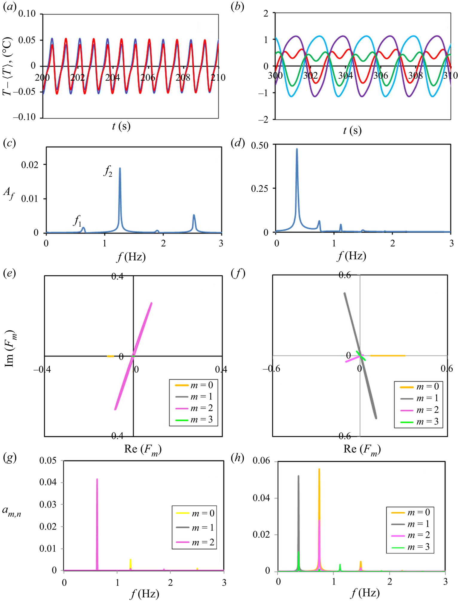
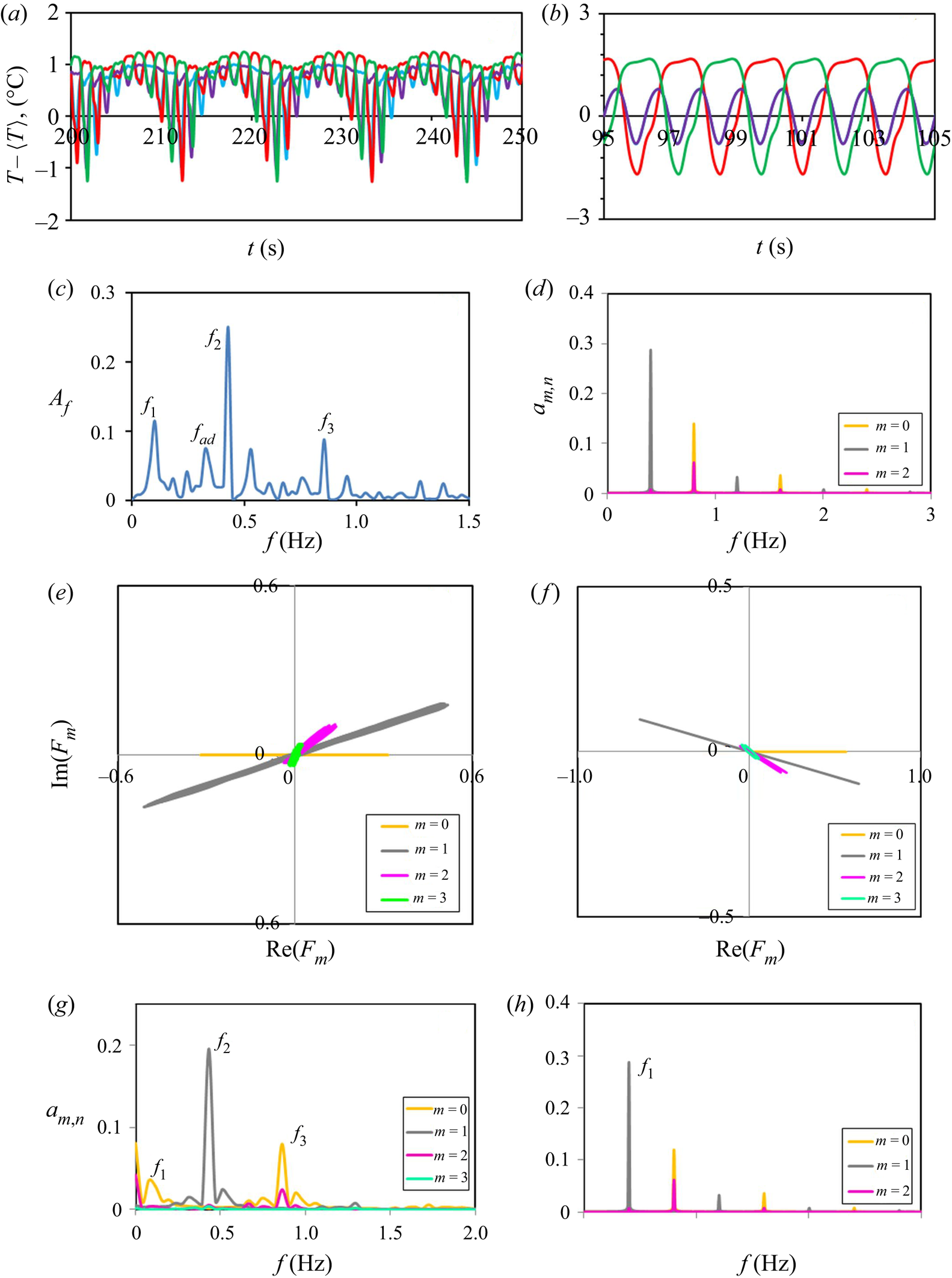
 $\tilde {T}_g$ are shown on the left side of figure 8. Figure 8(a) shows that the temperature signals are periodic with the presence of weak harmonics. Indeed, the temporal Fourier spectrum given in figure 8(c) reveals the presence of a subharmonic peak at
 $f_1=f_{2}/2=0.63\ \textrm {Hz}$. Another interesting observation from temperature oscillations is that all the signals from four observation points practically coincide. The simplest explanation could be that instability emerges as an axially TW
 $m=0$. However, the trajectory of the system in the phase plane, given in figure 8(e), clearly determines the dominant wavenumber
 $m=2$. Still, the presence of a wave with mode
 $m = 0$ can be seen in the phase plane when
 $-0.116<{Re}(F_0)<-0.096$.
(Path 1, numerical results.) Plots on the left side correspond to  $\tilde T_g=20\,^{\circ }\textrm {C}$ and on the right side to
 $\tilde {T}_g=28\,^{\circ }\textrm {C}$. (a,b) Temperature oscillations on four thermocouples. (c,d) Fourier spectrum. (e,f) Trajectories of the dynamic system. (g,h) Frequencies assigned to different modes and their amplitudes.

In order to better understand the HTW structure, the results of temporal Fourier analysis of the periodic function  ${Re}(F_m)$ are presented in figure 8(g). It reveals peaks of modes
 $m=0$ and
 $m=2$ at two first frequencies
 $f_1$ and
 $f_2$. The dominant mode
 $m=2$ has the largest peak at the frequency
 $f_1$ while the mode
 $m=0$ has the largest peak at the frequency
 $f_2.$ Thus, the most energetic mode is
 $m=0$ which determines the oscillations seen in figure 8(a). The closer inspection of these oscillations reveals small differences between the red and blue curves which are caused by the mode with
 $m=2$. It is visible that the red and blue maxima (tips) of oscillation curves alternate, i.e. the period of oscillations is actually two times bigger. That is the manifestation of the frequency
 $f_1=f_2/2$ produced by the mode
 $m=2$. It explains that in the plot for
 $a_{m,n}$, the mode
 $m=2$ is more energetic than the mode
 $m=0$. Finally, the solution for the HTW in this case can be written as
 \begin{equation} { F}=a_{0,1}\exp{(\textrm{i} \omega_2 t)}+ a_{2,1} \exp{(\textrm{i} \omega_1 t)}[\exp( \textrm{i} 2\varphi) + \exp(- \textrm{i} 2\varphi)] + \dots, \end{equation}
where  $|a_{0,1}|<|a_{2,1}|$ and
 $\omega _i=2{\rm \pi} f_i$.
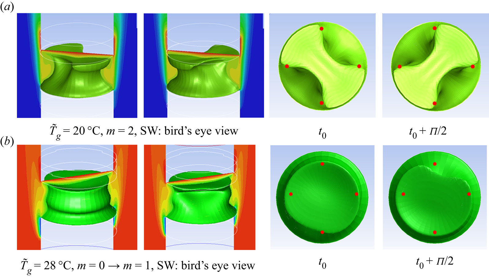
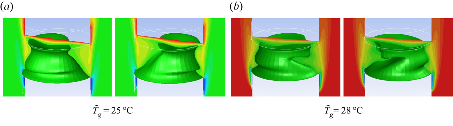
The above analysis demonstrated that instability develops as a SW with the predominant mode  $m = 2$, and this still leads to confusion with temperature fluctuations, which are identical at all four azimuthally equidistant points. In order to understand this puzzlement, the snapshots of a three-dimensional temperature field in bird's eye and top views are shown in figure 9(a) in two time moments shifted by half a period. The isosurfaces at
 $\tilde {T}_g=20\,^{\circ }\textrm {C}$ clearly identify a SW with mode
 $m=2$. The puzzle with temperature oscillations is disclosed by the top view of patterns presented next to isosurfaces, for simplicity they are shown only in the liquid phase. The temperature field has perfect azimuthal symmetry, and two consecutive images, taken with a difference of half of the period, display patterns shifted by
 $90^{\circ }$. All the numerical thermocouples, shown by the red dots, are located in the same phase of the wave. Supplementary movies 1 and 2 available at https://doi.org/10.1017/jfm.2020.901, ‘SWeyebirdview.avi’ and ‘SWtopview.avi’, present the temporal evolution of this highly symmetrical pattern in side and top views.
(Simulations, path 1  ${\rm \Delta} \tilde {T}=7\,^{\circ }\textrm {C},V_{g}=0.5\ \textrm {m}\ \textrm {s}$.) The flow pattern for the cases from figure 8. The first two pictures in each row show the isosurfaces of
 $\tilde T_{mean}=25\,^{\circ }\textrm {C}$ in the liquid phase embedded in a gas temperature field in the case of SWs for
 $m=2$ (a), and waves with mixed modes
 $m=0 + m=1$ (b). The gas temperature is shown by the colour palette, and the colour for
 $\tilde {T}_g=25\,^{\circ }\textrm {C}$ is identical to the liquid phase. The next two pictures present snapshots of the temperature field (top view) shifted by a half-oscillation period (
 $\varPi$) for the same modes of the isosurfaces. The red dots indicate the position of thermocouples in the liquid.

The isosurfaces shape in figure 9 also explains the possible difference in temperature readings on thermocouples located at the LB mid-height and in the experimental points at the top. The thermocouples set at the top and positioned on the petals of the three-dimensional image will record a higher amplitude than others. The four thermocouples in the LB mid-height are located not only on the thinnest part of the image but also on the border between the cold and hot spots, and register a lower amplitude than the others. According to a comparative Fourier analysis of the temperature signals in different locations, the set of frequencies is identical, but their Fourier amplitudes differ. It is worth noting that the results of all thermocouples, including the experimental one shown in figure 4(a,b), reveal a SW with the main frequency  $f_2 = 1.26$ Hz.
Next we examine the case when gas temperature is above the mean temperature, i.e.  $\tilde {T}_g=28\,^{\circ }\textrm {C}$. The characteristics of the temperature field for this case are detailed on the right side of figure 8. The amplitude of temperature oscillations in figure 8(b) is much larger in the case of hot gas. The FFT results in figure 8(d) illustrate the largest peak at
 $f=0.37$ Hz, noting a much lower frequency than at
 $T_g=20\,^{\circ }\textrm {C}$. The drop of the frequency indicates a possible change in the wave mode. The trajectories in the phase plane (see figure 8f) determine unambiguously the dominant azimuthal mode
 $m=1$, but the trajectory
 $F_0$ is strongly present when
 $0.07< {\rm Re}(F_0) <0.30$. The frequency analysis of
 $\textrm {Re}(F_m)(t)$ shown in figure 8(h) demonstrates that
 $m=1$ oscillates with the frequency
 $f=0.37$ Hz and has the largest amplitude among all the
 $a_{m,n}$ which is consistent with the FFT results, but the mode with
 $m=0$ is also energetic. The calculations in this case were long in time, more than three thermal times,
 $\tau _{th}=L^2/\chi = 107$ s. Figure 8 shows results at the very end, i.e.
 $t=330$ s while the flow structure was examined at different times. Two wavenumbers,
 $m=0$ and
 $m=1$, were observed at all times, but their role changed. At
 $t=90$ s, the prevailing mode was
 $m=0$ and it can be seen in the first three-dimensional isosurface of the mean temperature in figure 9(b). The temperature field is azimuthally symmetric. At
 $t=110$ s, the second isosurface, the mode
 $m=1$, acquires power and the isosurface loses azimuthal symmetry. From this moment onward, the instability evolves as a SW with the dominant mode
 $m=1$. This is also confirmed by the top view of the temperature patterns in figure 9, taken with a difference of half of the period at the end of observations. The solution for the HTW in this case can be written as
 \begin{equation} {F}=a_{0,1}\exp{(\textrm{i} \omega_2 t)}+ a_{2,1} \exp{(\textrm{i} \omega_1 t)}[\exp( \textrm{i}\varphi) + \exp(- \textrm{i}\varphi)] + \dots, \end{equation}
where  $|a_{0,1}|<|a_{2,1}|$ and
 $\omega _i=2{\rm \pi} f_i$.
Summing up on path 1, near the threshold, the hydrothermal instability emerges as a SW with several modes. With increasing gas temperature, the critical wavenumber changes from  $m=2$ to
 $m=1$. The presence of the secondary wave mode,
 $m=0$, increases with the gas temperature although it attenuates with time. Leypoldt et al. (Reference Leypoldt, Kuhlmann and Rath2000), dealing with
 $Pr=4$ and
 $Pr=7$, predicted that SWs decay to TWs. They also mentioned that close to the threshold, the former may persist for long times. Although the calculations for
 $\tilde {T}_g=28\,^{\circ }\textrm {C}$ were long in time we did not observe the decay of the SW. It is worth noting that the jump in the critical frequency at the mode change and even the ratio
 $f_{m=1}/f_{m=2}$ are in a good agreement with our recent experiments (Yasnou et al. Reference Yasnou, Gaponenko, Mialdun and Shevtsova2018).
6.3. Path 2
Path 2 traverses the stability window resulting in more complicated nonlinear dynamics; therefore, the largest number of points will be analysed along this path.
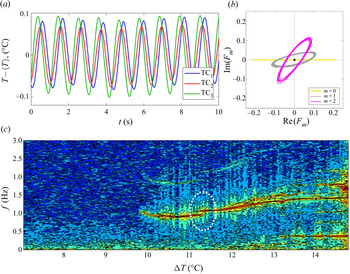
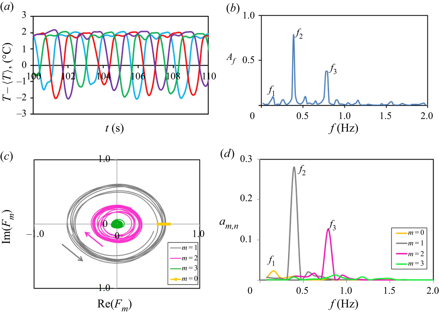
(Experiment, path 2.) In the experimental part, as in the case of path 1, the first point to consider is  $T_g=26\,^{\circ }\textrm {C}$, which is located close to the stability window. The temperature oscillations in figure 10(a) show that the maxima/minima on all three thermocouples occur almost simultaneously but their amplitudes are slightly different. It can correspond only to the azimuthal mode
 $m=2$ and, most likely, to a SW. In contrast, the trajectories of all azimuthal waves
 $m$ encircle the origin of a phase plane that could correspond to a TW. To resolve this mismatch, it can be assumed that the trajectories are deformed by noise because with three thermocouples we do not calculate the true Fourier harmonics. In addition, the amplitudes of the trajectories
 $F_1$ and
 $F_2$ are comparable that can suggest the coexistence of two modes. To offer additional physical explanation for the dynamics of the oscillatory system close to stabilization, the Fourier map is presented in figure 10(c). We would like to draw your attention to the area inside the white circle. The first observation from the selected area is the occurrence of a frequency skip. Second, there is a small range of
 ${\rm \Delta} T$ at which two independent frequencies coexist
 $f_1=0.96$ and
 $f_2=1.07$ Hz. Hence, there are two HTWs. We also noticed the presence of strong harmonics in the spectrum just before the jump in the fundamental frequency. This case calls for a complementary explanation by numerical modelling.
(Experimental results on path 2.) (a) Temperature oscillations on three non-equidistant thermocouples. (b) Trajectories of the system in a phase space. (c) The Fourier map at  $T_g=26\,^{\circ }\textrm {C}$,
 $V_g = 0.5\ \textrm {m}\ \textrm {s}^{-1}$ and
 ${\mathcal {V}} = 1.0$.

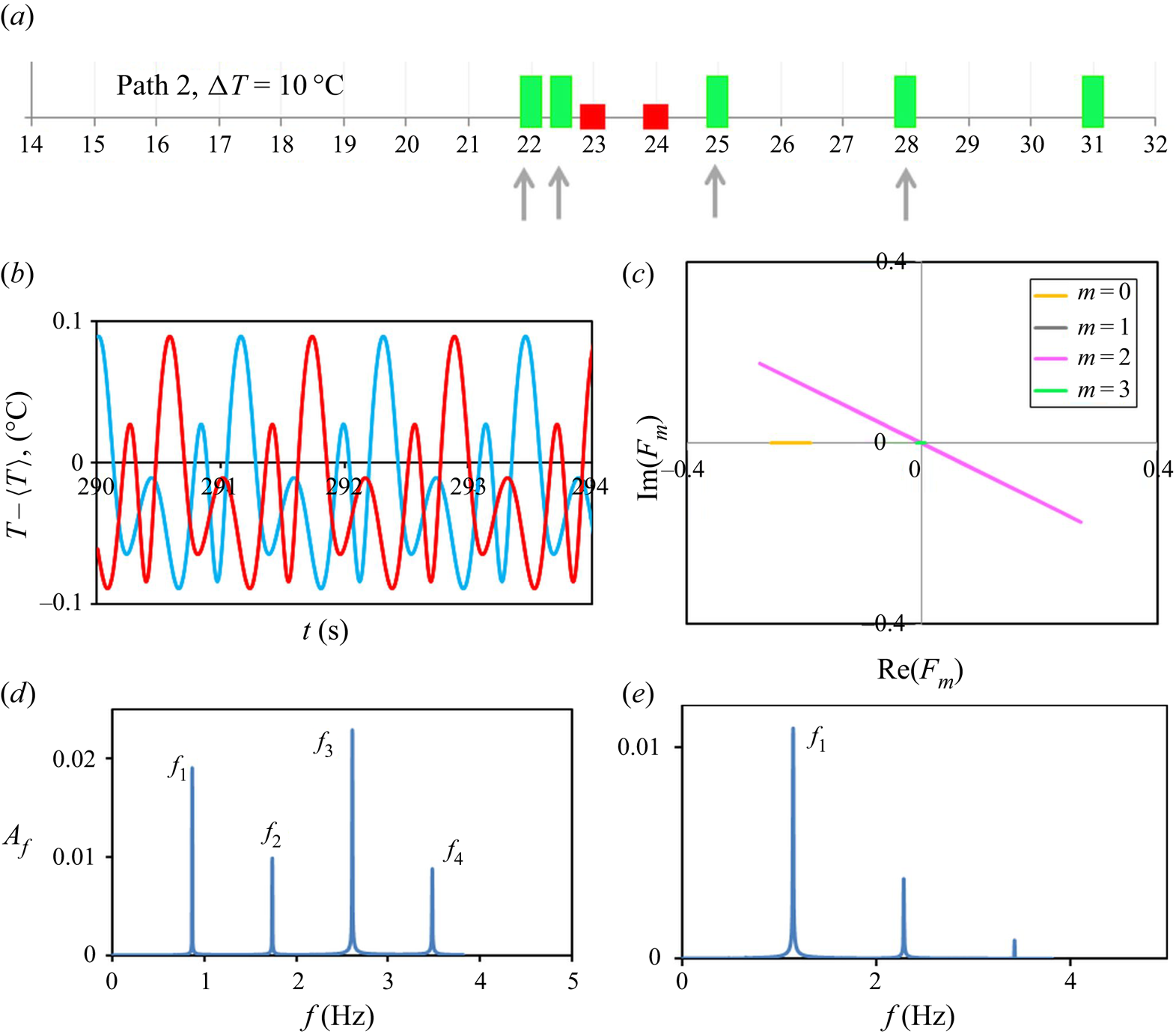
(Simulations, path 2.) The numerical simulations along path 2 at  ${\rm \Delta} \tilde {T}= 10\,^{\circ }\textrm {C}$ were conducted for seven gas temperatures, as shown in figure 11(a). Due to the complex behaviour of oscillatory states, the system will be analysed at four gas temperatures from both sides of the stability window but close to its location, they are
 $\tilde {T}_g=22\,^{\circ }\textrm {C}$,
 $\tilde {T}_g=22.5\,^{\circ }\textrm {C}$,
 $\tilde {T}_g=25\,^{\circ }\textrm {C}$ and
 $\tilde {T}_g=28\,^{\circ }\textrm {C}$. These points are indicated by small arrows in figure 11(a).
Numerical results on path 2 on the colder side of the stability window in a LB subjected to a parallel gas stream when  $U_g = 0.5\ \textrm {m}\ \textrm {s}^{-1}$,
 ${\rm \Delta} \tilde {T}=10\,^{\circ }\textrm {C}$. (a) The state points calculated along path 2. The arrows highlight the oscillatory states under detailed examination. (b) Time series,
 ${T_{g}}=22\,^{\circ }\textrm {C}$. (c) Phase trajectories,
 ${T_{g}}=22\,^{\circ }\textrm {C}$. (d) Fourier spectrum,
 ${T_{g}}=22\,^{\circ }\textrm {C}$. (e) Fourier spectrum,
 ${T_{g}}=22.5\,^{\circ }\textrm {C}$.

Time series at  $\tilde {T}_g=22\,^{\circ }\textrm {C}$ shown in figure 11(b) exhibit periodic behaviour, but represent a model that incorporates several harmonics. Further inspection shows that despite of four numerical thermocouples only two curves are visible. The temperature fluctuations recorded by two opposite thermocouples coincide. This is a clear sign that the HTW evolves in the form of a SW. Interestingly, the blue curve is exactly the red curve but shifted by half a period. That is rather unusual for a SW; such a behaviour would be natural for a TW. An explanation can be found in figure 9 (the last two subpanels in panel (a)), assuming that the patterns are rotated by
 $45^{\circ }$. The phase trajectories in figure 11(c) confirm a SW and determine a strongly dominant mode with
 $m=2$. The intricate time-dependent temperature behaviour on the one hand and the overwhelming single mode in the phase plane on the other hand create confusion. Besides, the numerical phase trajectories do not support the experimental ones indicating features of a TW.
Next, we examine the temporal Fourier spectrum of temperature oscillations which is shown in figure 11(d). Unlike the single-mode phase plane, the Fourier spectrum contains several frequencies of a comparable amplitude:  $f_1=0.87$,
 $f_2=2f_1$,
 $f_3=3f_1$ and
 $f_4=4f_1$. Intriguingly, the FFT amplitudes are non-monotonic:
 $A(\,f_1)=1.93\tilde {a}$,
 $A(\,f_2)=\tilde {a}$,
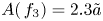 $A(\,f_3)=2.3\tilde {a}$, where
 $\tilde {a}=0.01\ \textrm {a.u.}$ The non-monotonic behaviour of the amplitude of the temporal Fourier harmonics
 $A(\,f_n)$ on
 $n$ provides a hint that there can be a certain synchronization of different modes with different characteristic frequencies. In line with experimental observations, it suggests that approaching the stability window the competition between wave modes is expected.
The complementary Fourier analysis of the function  $\textrm {Re}(F_m)(t)$ determined that the dominant mode
 $m=2$ is associated with frequency
 $f_1$ and the mode
 $m=0$ is associated with frequency
 $f_2$ of a very low amplitude (not shown here by graph). The temperature oscillations are strongly nonlinear, and the presence of the third harmonic
 $f_3$ is obvious. Finally, the solution for HTW in this case can be written as
 \begin{equation} {F}= a_{0,2}\exp{(\textrm{i} \omega_2 t}) + a_{2,1}\exp{( \textrm{i}\omega_1 t)} [\exp(\textrm{i}2 \varphi) + \exp(-\textrm{i}2 \varphi)] + \dots, \end{equation}
where  $|a_{2,1}|\gg |a_{02}|$ and
 $\omega _i=2{\rm \pi} f_i$.
To obtain additional insight on the dynamics of the system, the computer simulations were conducted for the gas temperature only half a degree higher, i.e.  $\tilde {T}_g=22.5\,^{\circ }\textrm {C}$. The temporal Fourier spectrum for this case is shown in figure 11(e), which is very different from the previous case. The amplitudes of the temporal Fourier harmonics
 $A(\,f_n)$ decrease monotonically. The amplitude of the temperature oscillations at
 $\tilde {T}_g=22.5\,^{\circ }\textrm {C}$ in figure 12(a) is significantly smaller than at
 $\tilde {T}_g=22.0\,^{\circ }\textrm {C}$, displaying attenuation of the oscillatory instability. Furthermore, these oscillations clearly demonstrate a TW: all signals have the same amplitude, and the extreme values are shifted by a quarter of the period. The phase trajectories at this gas temperature (figure 12b) resolve the nonlinear dynamics. First, it confirms that the dominant azimuthal mode has changed from
 $m=2$ to
 $m=1$. Second, it shows the strong presence of the previous mode,
 $m=2$. It is worth noting that both HTWs propagate in the same clockwise direction, and with the same phase velocity,
 $v_p=2{\rm \pi} f/m$. The amazing collective behaviour (spatial coherence) of waves in three-dimensional space is shown in complementary movie 3 ‘codirectedTW.avi’ through the spreading of the mean temperature isosurface. It can also be seen in the movie that the HTW propagates from the cold to the hot side as an oblique wave.
(Path 2.) (a) Temperature oscillations on three non-equidistant thermocouples. (b) Trajectory of the system in a phase space;  $\tilde {\Delta } T=10\,^{\circ }\textrm {C}$,
 $\tilde {T}_g=22.5\,^{\circ }\textrm {C}$,
 $V_g = 0.5\ \textrm {m}\ \textrm {s}^{-1}$ and
 ${\mathcal {V}}=1.0$.

Finding in simulations the bifurcation from a SW to a TW at the boundary of the stability window, we return to the occurrence of two experimental frequencies shown in figure 10(c). A change of the frequency  $f_1= 0.87$ Hz at
 $\tilde {T}_g=22.0\,^{\circ }\textrm {C}$ to 1.14 at
 $\tilde {T}_g=22.5\,^{\circ }\textrm {C}$ at the bifurcation leads to an analogy with the experimental observations. Here we would like to underline that both experimental and numerical analyses were able to recover the same nonlinear behaviour of the system on the boundary of the stabilization. They both demonstrate that SWs dominating over a large part of path 2 become unstable and decay to a TW before the stability window.
We now turn to examining the flow structure beyond the stability window. The evolution of the system is considered in detail at the point closest to the stability window,  $\tilde {T}_g=25\,^{\circ }\textrm {C}$, and slightly away,
 $\tilde {T}_g=28\,^{\circ }\textrm {C}$. The time series of temperature fluctuations are shown in figure 13(a,b). It follows that the oscillations amplitude is at least one order of magnitude larger than before the stability window (see figures 11 and 12) and increases further with the gas temperature. The shape of oscillations near the stability window, panel (a), reveals the presence of multiple frequencies. Indeed, the FFT analysis in panel (c) displays at least two independent frequencies
 $f_1= 0.01\ \textrm {Hz}$ and
 $f_2=0.43$ and their numerous combinations, for example,
 $f_3=2f_2$,
 $f_{ad}=f_2 - f_1$. The phase plane also exhibits a multimodal picture, but with a clearly dominant mode
 $m=1$. Driven by this multimodal behaviour with multiple frequencies in the spectrum, a Fourier analysis of
 $\textrm {Re}(F_m)(t)$ for different
 $m$ was carried out to assign the FFT frequencies to each mode. The results for this frequency analysis are shown in panel (g). Recall, that in the notation
 $a_{m,n}$ the first subscript is for the mode and the second for the frequency. In agreement with FFT results, the most energetic mode is
 $m=1$ oscillating at
 $f_2$. It appeared that the mode
 $m=0$ has two peaks. One peak is at
 $f_3=2f_2$, and that is just the nonlinear effect due to the coupling with the
 $m=1$ mode. Another peak of the mode
 $m=0$ is at the essentially lower frequency
 $f_1<f_2$, and this wave is responsible for the large oscillations period (beating) in figure 13(a). The equation for the HTW in this case can be written as
 \begin{equation} {F}=a_{0,1}\exp{(\textrm{i} \omega_1 t)}+a_{1,2} \exp{(\textrm{i} \omega_2 t})[\exp(\textrm{i} \varphi) + \exp(-\textrm{i} \varphi) ]+ a_{0,3}\exp{(\textrm{i} \omega_3 t})+ \dots, \end{equation}
where  $|a_{0,1}| < |a_{0,3}| < a_{1,2}$ and
 $\omega _i=2{\rm \pi} f_i$.
(Path 2 after stability window, simulations.) Left side corresponds to  $\tilde {T}_g=25\,^{\circ }\textrm {C}$, and right to
 $\tilde {T}_g=28\,^{\circ }\textrm {C}$, respectively. (a,b) Temperature oscillations on four thermocouples. (c,d) Trajectories of the system in a phase space. (e,f) Frequencies assigned to different modes and their amplitudes. (g,h) Frequencies assigned to different modes and their amplitudes.

The right side of figure 13 reveals the HTW properties slightly away from the stability window, at  $\tilde T_g=28\,^{\circ }\textrm {C}$. The temperature oscillations are more regular and the FFT spectrum displays a monotonic behaviour. Despite very different temporal Fourier spectra, the trajectories in the phase plane shown in figures 13(c) and 13(d) display strong similarities. In both cases,
 $\tilde {T}_g=25\,^{\circ }\textrm {C}$ and
 $\tilde {T}_g=28\,^{\circ }\textrm {C}$, the instability emerges as a SW with the dominant wavenumber
 $m=1$ and several other modes. Note, the axially running wave with
 $m=0$ is the second important mode and
 $m=2$ is clearly present.
The occurrence of enigmatic multimodal flow regimes after the stability window can be traced from the snapshots of the temperature field in figure 14. The isosurfaces of the mean temperature in the liquid, embedded in the general temperature field, are shown at two time instants shifted by half a period. The change in the slope of the isosurface after half the period is attributed to the wave mode  $m=1$, an additional wave-like movement from the bottom up can be attributed to
 $m=0$. Surely, the mode
 $m=2$ causes additional deformation of the surface, but it is almost invisible in these snapshots.
(Path 2 after stability window.) The isosurfaces of the mean temperature in the liquid ( $\tilde {T}=25\,^{\circ }\textrm {C}$) embedded in the general temperature field at
 $\tilde {T}_g=25\,^{\circ }\textrm {C}$ and
 $\tilde {T}_g=28\,^{\circ }\textrm {C}$. Two isosurfaces for the same
 $T_g$ are shifted by half of the period.

Summing up, experiments and computer simulations showed that after the stability window the increase of the gas temperature promotes the evolution of a SW with the dominant mode  $m=1$. The critical frequency strongly drops from
 $f=1.14$ Hz down to
 $f=0.43$ Hz at
 $\tilde {T}_g=25\,^{\circ }\textrm {C}$; a similar tendency was observed on path 1. With a further increase in
 $T_g$, the main frequency shows only a very slight increase.
6.4. Path 3
(Experiment, path 3.) The global experimental map (see figure 6) shows that path 3 passes above the stability window and, moving from the region of cold to hot gas, the system crosses various oscillatory states. In this supercritical region one can expect nonlinear interactions of different azimuthal modes. The complex coupling between different wave modes does not allow applying the analysis used above in a wide range of  $T_g.$ Observations reveal that when
 $T_g >T_{mean}$, temperature fluctuations in the liquid tend to a periodic function with a single frequency. The time evolution of temperature and the trajectories in the phase plane at
 $T_g=26\,^{\circ }\textrm {C}$ are shown in figure 15. The beatings in the temperature signals indicate the quasi-periodic regime. The mutual position of the maxima in temperature fluctuations (figure 15a) is more consistent with a SW or mixed waves. The trajectories in the phase plane (figure 15b) do not determine uniquely the prevailing wavenumber. The first observation is that all the trajectories are not closed and look as the projections of a multidimensional torus on a plane. The trajectory of the mode
 $m=2$ is round and more consistent with the TW while the mode
 $m=1$ resembles the ellipse. The ellipse can be formed as a result of a hypothetical solution composed of two TWs with different amplitudes,
 $|a_{1+}|\neq |a_{1-}|$. Then the trajectory for
 $m=1$ can be presented as
 \begin{equation} {F_1}=a_{1+}\exp{(\textrm{i} \omega t)}+a_{1-}\exp{(-\textrm{i} \omega t}) + \dots. \end{equation}
Alternatively, the ellipse can be formed by two SWs with a phase shift. Also, this kind of solution can appear due to secondary bifurcations from a TW towards a SW solution.
(Path 3, experiment.) (a) Temperature oscillations on three non-equidistant thermocouples. (b) Trajectories of the system in a phase space. Here  ${\rm \Delta} T=13\,^{\circ }\textrm {C}$,
 $T_g=26\,^{\circ }\textrm {C}$,
 $V_g = 0.5\ \textrm {m}\ \textrm {s}^{-1}$ and
 ${\mathcal {V}} = 1.0$.

(Simulations, path 3.) The simulations were carried out in four state points. At cooler gas,  $\tilde {T}_g \leqslant T_{mean},$ the signals are noisy, and the Fourier spectrum contains a bunch of harmonics. In agreement with the experiments, the signals become clearer with increasing gas temperature. Figure 16 unveils the HTW characteristics at
 $\tilde {T}_g=28\,^{\circ }\textrm {C}$. The time evolution of temperature signals in figure 16(a) shows that they are shifted by a quarter of a period, which means that instability develops in the form of a TW. But the oscillations are more complex than just a TW. The frequency spectrum in figure 16(b) displays several frequencies and it is similar to the FFT results on path 2 next to the stability window (see figure 13). This gives a hint that the system is close to the transition between oscillatory regimes. The phase plane in panel (b) defines the trajectory with the largest amplitude in the form of a TW with
 ${m=1}$. Furthermore, it also displays the existence of another TW with the wavenumber
 ${m=2}$. An intriguing aspect is that according to the time evolution of the phase trajectories, the wave of
 $m=1$ moves counterclockwise, and the wave of
 $m=2$ moves clockwise. The results of additional Fourier analysis of
 $\textrm {Re}(F_m)(t)$ presented in panel (c) are consistent with the above observations. The mode
 $m=1$ oscillating at the frequency
 $f_2=0.39$ Hz is the most energetic and its amplitude
 $a_{1,2}$ is two times larger than that of the mode
 $m=2$ oscillating at
 $f_3=2f_2$. The low frequency
 $f_1=0.142$ Hz with a small amplitude
 $a_{0,1}$ is assigned to the mode
 $m=0$.
(Path 3, simulations.) Here  $\tilde {{\rm \Delta} } T=13\,^{\circ }\textrm {C}$ and
 $\tilde {T}_g=28\,^{\circ }\textrm {C}$: (a) time evolution of temperature perturbations on four thermocouples. (b) Fast Fourier transform analysis. (c) Trajectories of the system in a phase space. (d) Frequencies assigned to different modes and their amplitudes.

Another interesting aspect is that the trajectories of both modes are not closed, as it was also seen in the experiments. This suggests that the centre of the cycle is continuously shifted. An explanation follows from the presence of the mode  $m=0$ which shifts the centre of the phase plane and provides filling between the two cycles. The illustration of the hydrothermal instability with an intriguing competition of the two TWs can be seen in movie 4 ‘oppositeTW.avi’. By definition, a TW is the translation without the change of the shape. In this case, in addition to certain total clockwise rotation, there is a significant change of the shape of isosurfaces. That is the result of the superposition of several waves moving in different directions.
7. Overview of the hydrothermal instability under action of gas flow
Figure 17(a) summarizes, in terms of gas temperature and applied thermal stress  ${\rm \Delta} T$, the different ways that a LB responds to forced gas motion along the interface. This diagram of HTW properties was obtained from numerical simulations but is fully consistent with the experimental observations, as shown above. The figure immediately reveals that SWs (purple bars) are the most common modes of instability. For the lower (path 1) and higher (path 3) values of thermal stress, there is no visible stability window but, instead, a mode transition occurs over a comparable region of gas temperatures. This suggests that the stability window shrinks as indicated.
Overview of the hydrothermal instability observed in a LB under the influence of a temperature gradient, gravity and forced gas flow:  $V_g=0.5\ \textrm {m}\ \textrm {s}^{-1}$,
 $\mathcal {V}=1$,
 $Pr=14$. (a) Map of the HTWs observed along different paths. The purple bars correspond to SWs, the light blue bars to TWs, the green bars to oscillatory states with a poorly defined structure and the red squares to stationary states. The grey shaded region indicates the stability window. The grey solid curve outlines the threshold of instability. (b) Evolution of the experimentally observed (filled symbols) and the numerically obtained (open symbols) frequency over the three selected paths.

The nonlinear dynamics associated with the HTWs can be classified into three regimes according to the dominant behaviour. (a) A SW with dominant azimuthal wavenumber  $m=2$ (other modes are of significantly lower amplitude) that is observed with cooler gas over a large range of
 ${\rm \Delta} T$. (b) A SW with dominant azimuthal wavenumber
 $m=1$ that is observed with hotter gas. (c) A region near the stability window where TWs or SWs can appear. We note that, in the first two regimes, we did not observe the transition from a SW to a TW predicted by Leypoldt et al. (Reference Leypoldt, Kuhlmann and Rath2000) for
 $Pr=4$ and
 $Pr=7$.
The instability in the latter regime is manifested in the form of superposition of several HTWs with different wavenumbers and bifurcations from SWs to TWs or vice versa take place. Approaching the stability window, a superposition of SWs with different characteristic frequencies appears on path 2, followed by a bifurcation to a TW. Although the TW occurs with the predominant mode  $m = 1$, it is accompanied by a secondary mode
 $m = 2$, and both rotate in a clockwise direction. Another TW is observed on path 3 after the stability window, compressed into an imaginary line. This TW also occurs with prevailing mode
 $m=1$ and a secondary mode
 $m = 2$. Intriguingly, they rotate in opposite directions.
The evolution of the dominant frequency along the three selected paths is shown in figure 17(b). This figure combines data from experiments and numerical simulations, which are in good agreement. In order to make this quantitative comparison, we shifted  $\tilde {T}_g$ from the numerical simulations by four degrees, as discussed in § 6.1. As the temperature of the gas rises, the dominant frequency of the
 $m=2$ mode gradually increases, reaching
 $f\sim 1.1\text {--}1.2$ Hz close to the stability window. The frequency drops significantly following the mode change, down to
 $f\sim 0.4$ Hz. Beyond this mode transition, the dominant frequency does not change appreciably over the range of gas temperatures considered.
8. Conclusions
Using carefully conducted experiments and simulations, we have demonstrated the importance of the temperature of a gas moving along a LB interface at a constant velocity for the hydrothermal instability. The working fluids were  $n$-decane (liquid) and nitrogen (gas),
 $Pr= 14$ and
 $Pr=0.7$, respectively. It was experimentally shown (Yasnou et al. Reference Yasnou, Gaponenko, Mialdun and Shevtsova2018) that, at certain gas temperatures, instability decays, forming a stability window. The presence and width of the stability window depends not only on the gas temperature, but also on how far the system is from the onset of instability, in terms of applied thermal stress
 ${\rm \Delta} T$. The stability window, when it exists, starts at
 ${\rm \Delta} T \sim 1.2 {\rm \Delta} T_{cr}$ and ends at
 ${\rm \Delta} T \sim 1.5\text {--}1.8 {\rm \Delta} T_{cr}$, where
 ${\rm \Delta} T_{cr}$ is the temperature difference marking the beginning of the instability region. Therefore, the study was carried out to trace the evolution of HTWs in LB with increasing gas temperature along three distinct constant values of
 ${\rm \Delta} T$, i.e. three different paths: path 1 follows just above the threshold of instability, path 2 traverses the stability window and path 3 goes above the stability window. Along each path, we investigate the development of HTWs in terms of prevailing and secondary azimuthal wavenumbers, in the form of SWs and TWs, as well as their coupling.
Throughout this study, the gas velocity was kept constant,  $V_g=0.5\ \textrm {m}\ \textrm {s}^{-1}$, and it moves starting from the cold side of the LB. Cooling by gas provides a stabilizing effect, as can be seen on the experimental map in figure 6 at low
 $T_g$. At large values of the heat flux, when the gas temperature is low, the primary effect of the moving gas is due to heat transfer, since shear stresses are weak due to a large viscosity ratio. As the gas temperature rises, hence approaching the mean temperature of the liquid, the heat flux consequently decreases, and its interplay with shear stresses becomes important for the stability of the flow, as both effects tend to become equally small. For example, the threshold starts exhibiting small alterations visible in figure 6. Above the threshold, this interaction becomes more complex and leads to the formation of a stability window.
The present work is focused on the properties of the HTWs. In this regard, the influence of the gas flow is manifested in the fact that HTWs emerge as a combination of at least two azimuthal modes, and one of them is  $m=0$. Another observation is that the SWs in the LB largely prevail over the TWs in the considered ranges of
 $T_g$. A selection of the preferred mode of instability is influenced by the gas temperature. Three regimes were identified according to the selection of HTWs. The standing HTW with the azimuthal wavenumber
 $m=2$ dominates in the region of cooler gas. Another SW with the azimuthal wavenumber
 $m=1$ dominates in the region of hotter gas. The most intriguing nonlinear dynamics occurs around the stability window, or on its extension by an imaginary line; it plays the role of a boundary between the two previous regimes.
We have paid special attention to the nonlinear evolution of HTW by means of Fourier analyses, by building trajectories of different modes in the phase plane, and making secondary Fourier analyses of these trajectories to relate the observed aziumuthal modes with the frequency in the Fourier spectrum. In some cases we also provide the mathematical equation describing HTW.
The change of the regimes is the most demonstrative while considering the nonlinear dynamics along path 2. Close to the stability window, an experimentally obtained Fourier map showed the coexistence of two independent frequencies with an approximately 10 % difference in values. The temperature readings from three thermocouples vaguely resembled a TW. In contrast, the numerical simulations reveal a SW with a strongly dominant mode at  $m=2$. The FFT amplitudes of multiple harmonics in the spectrum displayed a non-monotonic behaviour that provides a hint to a possible synchronization of different modes with different characteristic frequencies. Simulations at slightly higher gas temperature, just at the edge of the stability window, reveal the bifurcation from a SW with
 $m=2$ to a TW with
 $m=1$, but with the strong presence of the previous mode,
 $m=2$, and weaker appearance of mode
 $m=0$. Furthermore, both TWs propagate in the same clockwise direction being distorted by the presence of a non-rotating wave with
 $m=0$. This is also a good example that both approaches, experimental and numerical, provide valuable and consistent insights into the spatial organization of HTWs.
Immediately after the stability window the system selects again a SW as the preferred form of instability but with  $m=1$. It is worth noting that the HTW instability sets in as a multimodal wave at path 1 and path 2. However, on path 3, instability emerges in the form of a TW, somewhat similar to path 2, but before the stability window. As expected, similar to path 2, the TW has the preferred mode
 $m=1$ with strong presence of the mode,
 $m=2$, and weaker appearance of modes
 $m=0$ and
 $m=3$. In contrast, the TW of
 $m=1$ moves counterclockwise, and the wave of
 $m=2$ moves clockwise. The time evolution of the temperature isosurfaces shows that the dominant mode
 $m=1$ imposes total clockwise rotation, but with a significant change of the shape of isosurfaces in course of time due to the superposition of several waves moving in different directions.
Based on the consistency of the experimental and numerical results, it is shown that a LB system above  ${\rm \Delta} T_{cr }$ can be stabilized by the varying gas temperature. The identification of the stability window within the JEREMI experiment will not be the only benefit of the study. It will bring other additional values to the experiment. Notably, throughout the study, we have developed an original methodology for analysis of HTWs, which will be highly useful for analysis of the forthcoming JEREMI experiment.
Acknowledgements
The work of ULB team was supported by the PRODEX programme of the Belgian Federal Science Policy Office. A.N. acknowledges the support by the Israel Science Foundation (grant no. 843/18). We also thank J. Porter for helpful discussions.
Declaration of interests
The authors report no conflict of interest.
Supplementary movies
Supplementary movies are available at https://doi.org/10.1017/jfm.2020.901.