I. INTRODUCTION
Dielectric materials can develop accumulated charge under both plasma and radiation exposure. The charge distribution in dielectric materials generates self-consistent electric fields. These can change the electrical properties of the dielectric and are often responsible for dielectric breakdown. Measuring the physical locations of these charges can help to determine the mechanisms for charge accumulation and identify the steps to be undertaken to mitigate the charging and prevent dielectric breakdown.
It is easy to measure the charge distribution along the surface of a thin dielectric film. Reference Ren, Nishi and Shohet1 However, measuring the distribution perpendicular to the surface is much more challenging, especially as the thickness of the film decreases into the submicron range. Potential measurement techniques have been studied since the 1970s, and several different methods have been developed. Reference Ahmed and Srinivas2 A list and comparison of these methods can be found in Ref. Reference Collins3. These methods can be generally divided into two branches, thermal Reference Ahmed and Srinivas2,Reference Lang and Das-Gupta4,Reference Cheri, Abou Dakka and Toureille5 and acoustic methods. Reference Alquie, Dreyfus and Lewiner6,Reference Sessler, West and Gerhard7 The thermal methods, first proposed by Collins, consist of applying a thermal pulse on the surface of the dielectric film and measuring the response of the electric signal from the sample that contains charge distribution information. In acoustic methods, an ultrasonic pulse is excited and propagates through the sample. The pressure wave or acoustic pulse is used to excite electrical signals that contain charge distribution information or the acoustic signal itself contains such information. One of the most common acoustic techniques is the pulsed electro-acoustic (PEA) method. Reference Takada and Sakai8–Reference Li and Takada11 This uses a high-voltage (HV) narrow-width pulsed signal that is applied across the thickness of the film. This produces a mechanical pulse on the charges embedded in the dielectric. As a result, these charges oscillate and, in so doing, mechanical (acoustic) vibrations are excited. They are typically detected by a transducer on one side of the dielectric. By measuring the arrival time and magnitude of these vibrations, it is possible to deconvolve the transducer signal and relate it to the magnitude and location of the charges in the dielectric. Up to the present time, the spatial thickness resolution of this system has been of the order of 10 μm. Reference Maeno and Fukunaga12,Reference Bamji, Abou Dakka and Bulinski13
The goal of this work is to investigate the response of a charged dielectric film system to a simpler excitation—a single-frequency sinusoidal signal rather than a pulse. This technique is much easier to implement and it is not affected by dispersion of the acoustic wave. We also hypothesize that it can measure the relative charge amount with higher sensitivity than the PEA method. In addition, if the frequency is varied, the transfer function of the system can be obtained, allowing for the development of a more accurate algorithm for deconvolving the acoustic signal when the PEA method is utilized. Thus, instead of using a HV narrow pulse in the PEA system, we use a HV sinusoidal signal as the electrical input. This is called the sinusoidal electro-acoustic (SEA) method. Here, we examine its experimental response to a sinusoidal excitation and determine whether it is possible to measure the amplitude and location of volume charges located inside the dielectric film.
II. THEORY
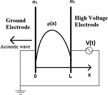
The analysis begins by examining two parallel plates with a dielectric film in between (Fig. 1). The thickness of the dielectric is L. The charge distribution in the dielectric film is described by a charge density function ρ(x). For simplicity, the charge density is assumed to be uniformly parallel to the plates. The input signal is V(t), where t is the time. An acoustic sensor is placed on the left side as shown in Fig. 1 to measure the acoustic pressure as a function of time.
Theoretical model for the SEA measurement. The dielectric with a continuous charge distribution of ρ(x) is between two electrodes with a high voltage sinusoidal signal applied. The acoustic sensor is on the left side of the grounded electrodes.

The surface charge densities on the electrodes are σ1(t) and σ2(t), for the grounded electrode and the HV electrode, respectively. Using charge neutrality and Gauss' law, we can obtain the charge density on the electrodes at any given time. To do so, we assume the RC charging time of the capacitor is much shorter than the period of the input sinusoidal signal. Here R is the resistance of the circuit and C is the capacitance of the parallel capacitor structure. Then, the expressions for the charge density on the electrodes as a function of time are Reference Maeno and Fukunaga12 :
 $${{\rm{\sigma }}_1}(t) = - {\rm{\varepsilon }}{{V(t)} \over L} - \int_0^L {{{L - x} \over L}{\rm{\rho }}(x){\rm{d}}x} \quad ,$$
 $${{\rm{\sigma }}_2}(t) = - \int_0^L {{x \over L}{\rm{\rho }}(x){\rm{d}}x} + {\rm{\varepsilon }}{{V(t)} \over L}\quad ,$$
where ε is the dielectric constant of the testing material. The electric field can be calculated from Gauss' law to be
 $$E(x,t) = {1 \over {\rm{\varepsilon }}}\int_0^x {{\rm{\rho }}(y){\rm{d}}y} - {1 \over {{\rm{\varepsilon }}L}}\int_0^L {{\rm{d}}x\int_0^x {{\rm{\rho }}(y){\rm{d}}y} } - {{V(t)} \over L}\quad .$$
The acoustic pressures generated by the electrodes are
 $${p_1}(t) = {{{\rm{\sigma }}_1^2(t)} \over {2{\rm{\varepsilon }}}} = {1 \over 2}{\rm{\varepsilon }}{{{V^2}(t)} \over {{L^2}}} + {1 \over {2{\rm{\varepsilon }}}}{\left[ {\int_0^L {{{L - x} \over L}{\rm{\rho }}(x){\rm{d}}x} } \right]^2} + {{V(t)} \over L}\int_0^L {{{L - x} \over L}{\rm{\rho }}(x){\rm{d}}x} \quad ,$$
 $${p_2}(t) = - {{{\rm{\sigma }}_2^2(t)} \over {2{\rm{\varepsilon }}}} = - {1 \over 2}{\rm{\varepsilon }}{{{V^2}(t)} \over {{L^2}}} - {1 \over {2{\rm{\varepsilon }}}}{\left[ {\int_0^L {{x \over L}{\rm{\rho }}(x){\rm{d}}x} } \right]^2} + {{V(t)} \over L}\int_0^L {{x \over L}{\rm{\rho }}(x){\rm{d}}x} \quad .$$
The contribution to the pressure wave from the dielectric charge located at position x is
 $${\rm{d}}{p_0}(x,t) = - {{V(t)} \over L}{\rm{\rho }}(x){\rm{d}}x\quad .$$
The acoustic wave arriving at the sensor is a combination of two parts, Reference Ren, Nishi and Shohet1 the acoustic wave from the volume charge in the dielectric and Reference Ahmed and Srinivas2 the acoustic wave from the two electrodes. Acoustic waves that originate from different locations arrive at the sensor at different times, resulting in time delays or phase shifts if the V(t) is a sinusoidal function. If the attenuation and dispersion of the acoustic wave can be neglected, the net acoustic wave as a function of time at the sensor can be written as
 $${p_{{\rm{tot}}}}(t) = {p_1}(t) + {T^2}{p_2}(t - L/c) - T\int_0^L {{{V(t - x/c)} \over L}{\rm{\rho }}(x){\rm{d}}x} \quad ,$$
where c is the speed of sound in the dielectric and T is the transmission coefficient at the boundary (we assume when the acoustic wave passes through the boundaries of different materials, its amplitude changes by a factor of T). In Eq. (7), the first two terms are from the electrodes and the last term is from the volume charge. The power of T on each of the terms in Eq. (7) is determined by the number of layers that the acoustic signal must traverse. The transmission coefficient is assumed to be the same for signals traveling from material A to material B or from material B to material A.
A. Pulse input
In the PEA system, the input signal is a HV narrow pulse. If the width of the pulse is short enough, it can be assumed to be a delta function,
 $$V(t) = {V_0}{\rm{\delta }}(t)\quad ,$$
where V 0 is the amplitude of the pulse. Placing this input function into Eq. (7), we get
 $${p_{{\rm{tot}}}}(t) = {K_1}{\rm{\delta }}(t) + {K_2}{\rm{\delta }}(t - L/c) + T{V_0}{\rm{\rho }}(ct)\quad ,$$
where K 1 and K 2 are two parameters related to the charge density on the electrodes. We can see that the first two terms in Eq. (9) are two pulse signals that are time separated from the last term that contains the charge-distribution information. We examine the last term for further analysis.
 $$p(t) = T\int_0^L {{{{V_0}} \over L}{\rm{\delta }}\left( {t - {x \over c}} \right){\rm{\rho }}(x){\rm{d}}x = {{{{TV} \over L}}_0}} \rho (x = ct)\quad .$$
Based on Eq. (10), the charge density function can be written as
 $${\rm{\rho }}(x) = {{p\left( {t = {x \over c}} \right)} \over {TV_0 }}\quad .$$
However, p(t) cannot be directly measured because it is convolved with the dielectric and the detection system. As a result, the acoustic wave will travel through the system and can be detected by a frequency-dependent sensor (usually a piezo-electric sensor). Consider the output from the sensor in the frequency domain to be
 $${V_{{\rm{out}}}}({\rm{\omega }}) = P({\rm{\omega }})H({\rm{\omega }})K({\rm{\omega }})\quad ,$$
where H(ω) is the transfer function of the sensor and K(ω) is the transfer function of the system. If these two functions are known, we can obtain
 $$P({\rm{\omega }}) = {{{V_{{\rm{out}}}}({\rm{\omega }})} \over {H({\rm{\omega }})K({\rm{\omega }})}}\quad .$$
Then, we can take the inverse Fourier transform of P(ω) and get the charge distribution function using Eq. (11).
B. Sinusoidal input
For the SEA system, the input signal is sinusoidal with an amplitude of V 0 and an angular frequency ω. Therefore
 $$V(t) = {V_0}\exp (i{\rm{\omega }}t)\quad ,$$
 $${p_1}(t) = {{{\rm{\sigma }}_1^2(t)} \over {2{\rm{\varepsilon }}}} = {{{\rm{\varepsilon }}{V_0}^2\exp (i2{\rm{\omega }}t)} \over {2{L^2}}} + {{{V_0}\exp (i{\rm{\omega }}t)} \over L}\int_0^L {{{L - x} \over L}{\rm{\rho }}(x){\rm{d}}x} + {1 \over {2{\rm{\varepsilon }}}}{\left[ {\int_0^L {{{L - x} \over L}{\rm{\rho }}(x){\rm{d}}x} } \right]^2} + {{{\rm{\varepsilon }}{V_0}^2} \over {4{L^2}}}\quad ,$$
 $${p_2}(t) = - {{{\rm{\sigma }}_2^2(t)} \over {2{\rm{\varepsilon }}}} = - {{{\rm{\varepsilon }}{V_0}^2\exp (i2{\rm{\omega }}t)} \over {2{L^2}}} + {{{V_0}\exp (i{\rm{\omega }}t)} \over L}\int_0^L {{x \over L}{\rm{\rho }}(x){\rm{d}}x} - {1 \over {2{\rm{\varepsilon }}}}{\left[ {\int_0^L {{x \over L}{\rm{\rho }}(x){\rm{d}}x} } \right]^2} - {{{\rm{\varepsilon }}{V_0}^2} \over {4L}}\quad ,$$
 $${\rm{d}}p = - {{{V_0}\exp (i{\rm{\omega }}t)} \over L}{\rm{\rho }}(x){\rm{d}}x\quad .$$
We can see that the terms in Eqs. (15)–(17) have dc components as well as first and second harmonic components. The second harmonic term is not dependent on the charge distribution. Thus, we must consider only the first harmonic components in using this method. After including the time delay, we get the first harmonic amplitude of the wave at the location of the sensor to be
 $${A_{1{\rm{st}}}}= {{{V_0}} \over L}\bigg[ {\int_0^L {{{L - x} \over L}{\rm{\rho }}(x){\rm{d}}x} + {e^{i{\rm{\omega }}{L \over c}}}\,{T^2}\int_0^L {{x \over L}{\rm{\rho }}(x){\rm{d}}x} - T\int_0^L {{e^{i{\rm{\omega }}{x \over c}}}{\rm{\rho }}(x){\rm{d}}x} \bigg]\quad .$$
If the charge is a single layer, ρ(x) = σ0 δ(x–x 0), then
 $${A_{{\rm{1st}}}} = {{{V_0}} \over L}{{\rm{\sigma }}_0}\left[ {1 - {{{x_0}} \over L} + {T^2}{{{x_0}} \over L}{e^{i{\rm{\omega }}{L \over c}}} - T{e^{i{\rm{\omega }}{{{x_0}} \over c}}}} \right]\quad .$$
We can see that the first harmonic amplitude is proportional to the charge density, and the phase of the first harmonics is determined by the location of the charge. The expression for the phase angle is
 $${\phi _{{\rm{1st}}}} = {\tan ^{ - 1}}\left[ {{{{T^2}{{{x_0}} \over L}\sin \left( {{\rm{\omega }}{L \over c}} \right) - T\sin \left( {{\rm{\omega }}{{{x_0}} \over c}} \right)} \over {1 - {{{x_0}} \over L} + {T^2}{{{x_0}} \over L}\cos \left( {{\rm{\omega }}{L \over c}} \right) - T\cos \left( {{\rm{\omega }}{{{x_0}} \over c}} \right)}}} \right]\quad .$$
At a low frequency,
 ${\rm{\omega\, }}{\textstyle{L \over c}} \ll 1$
, where c is the speed of the acoustic wave in the dielectric material, the exponentials can be replaced by the first three terms in their Taylor expansion to be
 $\exp (i{\rm{\omega }}x/c) \approx 1 + \left( {i{\rm{\omega }}x/c} \right) - (1/2){({\rm{\omega }}x/c)^2}$
.
 $${A_{{\rm{1st}}}} = {{{V_0}} \over L}{{{{\rm{\omega }}^2}} \over {2{c^2}}}\left[ {\int\limits_0^L {{\rm{\rho }}(x)({x^2} - Lx){\rm{d}}x} } \right] \approx {{{V_0}} \over L}{{{{\rm{\omega }}^2}} \over {2{c^2}}}{{\rm{\rho }}_{{\rm{avg}}}}{x_{{\rm{avg}}}}(L - {x_{{\rm{avg}}}})\quad \,\,\,{\phi _{{\rm{1st}}}} = {\rm{\omega }}{{L + {x_0}} \over {3c}}\quad ,$$
setting T = 1. In Eq. (21), the average charge density (ρavg) and average position of the charge (x avg) are defined as
 $${{\rm{\rho }}_{{\rm{avg}}}} = {1 \over L}\int\limits_0^L {{\rm{\rho }}(x){\rm{d}}x} \quad ,$$
 $${x_{{\rm{avg}}}} = {{\int\limits_0^L {x{\rm{\rho }}(x){\rm{d}}x} } \over {\int\limits_0^L {{\rm{\rho }}(x){\rm{d}}x} }}\quad ,$$
From Eq. (21), we see that the first harmonic amplitude of the signal from the sensor is proportional to the average charge density and is also related to the average position of the charge. Equation (21) is valid for the experimental conditions reported here.
C. Examples
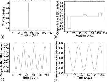
Consider a very simple charge distribution with only one layer of charge at the center, as shown in Fig. 2(a). The distribution function can be written as
 $${\rm{\rho }}(x) = \left\{ {\matrix{ {{\rm{\rho }}_0 \quad\matrix{ {} {x \in \left[ {{L \over 2} - {a \over 2},{L \over 2} + {a \over 2}} \right]} \cr } } \cr {0_{\quad\quad\quad} \matrix{ {\matrix{ {} {} \cr } } {} \cr } \matrix{ {} {{\rm{otherwise}}} \cr } } \cr } } \right.\quad ,$$
where a is the thickness of the layer and ρ0 is a constant.
Simulation of PEA and SEA methods with a single layer charge distribution: (a) the charge distribution; (b) the output signal from of the PEA method; (c) the output signal from the SEA method; and (d) the modified output signal from SEA method with the second harmonic removed.

We now estimate what the output would be like for both the PEA and SEA methods. Under ideal PEA conditions (no dispersion, perfect sensor, instant continuous data acquisition) with an input signal as pulse described as
 $$V\left( t \right) = \left\{ {\matrix{ {V_0 \quad\matrix{ {} {t \in [0,T]} \cr } } \cr {0\matrix{ {} {\matrix{ {} \quad{{\rm{otherwise}}} \cr } } \cr } } \cr } } \right.\quad ,$$
the output is shown in Fig. 2(b). The measured charge distribution has two peaks corresponding to the induced charge on the electrodes. The rectangular charge distribution was measured as a trapezoid and is wider than the real distribution. The reason for the widening effect is that the input pulse is not a true delta function and the width of the measured distribution is proportional to the width of the pulse.
Using the SEA method, the input will become a sinusoidally varying signal as shown in Eq. (14). The output for the low frequency case is shown in Fig. 2(c). These results will be shown to match the experimental conditions. Because only the first harmonic component in the output is informative, the second harmonics in the actual output were filtered out and the modified signal is shown in Fig. 2(d).
D. Comparison of the PEA and SEA methods
The main advantage of the PEA method is that it can measure the spatial charge distribution function. A number of difficulties appear however. First, as seen in Eq. (9), the charge distribution near the surface of the film is mixed with the signal from the electrodes and therefore cannot be measured explicitly. Second, the PEA measurement is based on the assumption that the attenuation and dispersion of the wave is not significant. However, at high frequencies (more than 100 MHz), the attenuation and dispersion of the acoustic wave can be very large and will cause a significant distortion of the output signal. The response of the piezo-electric sensor also becomes very small at high frequencies. Third, as shown in Eq. (13), the analysis of the PEA method requires knowing the frequency transfer-function of the system assuming of course, that it is linear. This is often difficult to find.
The low-frequency SEA method can detect the average amount of charge. At high frequencies, the phase of the output signal contains the information on the location of the charge. Compared with the PEA method, the SEA method is much easier to set up, since it does not require a very short pulse of high voltage and a fast-response acoustic sensor. In addition, the SEA method uses a single frequency at a time, so the problems of dispersion and the lack of knowledge of the transfer-function of the system do not apply. In addition, by varying the frequency using the SEA method, the frequency transfer function can in fact be obtained, which provides a possible improvement to the PEA method.
III. EXPERIMENTAL CONFIGURATION
In this work, the SEA method was applied to Kapton and high-density polyethylene (HDPE) films. The thickness of the films was between 50 and 150 μm. Copper foils were inserted between the dielectric layers and charged up to simulate charged layers in the film. Dielectric films with single and multiple charged-layer conditions were investigated.
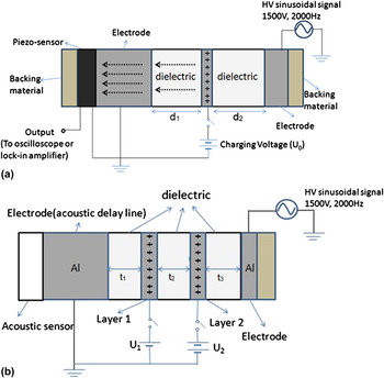
The experimental setup is shown in Fig. 3. Figure 3(a) shows two layers of Kapton dielectric. Initially, a 50-μm thick copper foil was inserted between the two pieces of a Kapton film. The copper foil was charged by connecting a d.c. voltage source (U 0) to the copper foil to produce a layer of controllable charge. After the potential reached a steady state, the d.c. supply was disconnected from the foil so as to simulate a constant-charge situation. A Wavetek 19 function generator (San Diego, CA) was used to generate the sinusoidal signal and a Trek 609D-6 HV amplifier (Trek Corporation, Lockport, NY) was used to amplify the signal. A sinusoidal voltage (1–10 kHz, 1–4 kV Vpp) is applied across both of dielectric films. A piezoelectric sensor (SDT1-028K) that measures the acoustic signal is attached to the grounded electrode. Two thick rubber sheets (3 mm) are placed as backing layers on both sides of the whole system so as to absorb the acoustic waves and prevent reflections. All the films and parts were clamped together to make good mechanical contact.
The experiment setup for SEA measurement. Copper layers are inserted to simulate the layers of charge. (a) Measurement with a single layer of charge. The location of the charging layer can be controlled by changing the values of d 1 and d 2. The charge density is controlled by the d.c. voltage source U 0. (b) Measurement with two layers of charge. The locations of the charging layers are controlled by t 1, t 2, and t 3. The charge density is controlled by the d.c. voltage sources U 1 and U 2.

To simulate multiple charge layers, more than one copper foil was used, as shown in Fig. 3(b). Each of the copper layers was connected to a d.c. voltage source to control its charge density.
The sinusoidal signal applied to the dielectric material generates a time-varying electric field inside the dielectric layers. The electric field then acts on the charges on the electrodes and the copper foil, causing them to vibrate and thus generate acoustic waves that propagate through the dielectric so as to reach the piezo transducer. The output of the piezo-electric transducer was connected to a lock-in amplifier (SR810) and an oscilloscope (HP 54820A) to analyze the signal.
The charge on the copper foil decays with time from leakage currents in the dielectric with an RC time constant. Both the theoretical RC time calculation and experimental data show that the charge can stay on the copper foil for around 10 s. We can easily control the amount of charge by changing the d.c. charging voltage U 0. In this experiment, U 0 was varied between 0 and 1500 V.
Initially, it was found that in order to have a measurable acoustic signal, the sinusoidal input signal should have an amplitude of 500 V or larger. The amplitude of the output signal varies slowly with the frequency of the input sinusoidal signal. The frequency was initially set to 1.5 kHz where the signal output was a maximum.
IV. EXPERIMENTAL MEASUREMENTS
A. Harmonic components of output signal
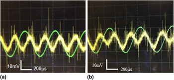
The output is a mixture of first and second harmonics of the input frequency, as explained earlier. The piezoelectric signal from a clean dielectric film (without any volume charge) is shown in Fig. 4(a). As described previously, the output signal has twice the frequency of the input signal. This is because the outer electrodes become alternately positively and negatively charged, but the mechanical force always acts so as to attract them. Both the charge on the electrodes and the electric field vary sinusoidally. The acoustic signal, generated by the electrodes, being proportional to the product of charge and field, has therefore twice the frequency of the input signal.
Signal from the piezo sensor and the input signal for different situations. The thinner curves are the input signals from the HV source. The thicker curves are the signal from the piezo-sensor. (a) No charge inside the dielectric. (b) There is a positive charge inside the dielectric.

When charge is placed on the floating layer, the output signal is as shown in Fig. 4(b). The combined signal is now composed of both the first and second harmonics. Since the charge on the floating electrode is assumed to always be of the same sign, the force on this electrode follows the first harmonic, while the second harmonic from the electrodes still exists. This is consistent with the analysis developed above.
B. Measurement with a single floating-charge layer
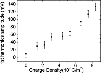
Using the setup in Fig. 3, the amount of charge in the floating layer was changed and the first harmonic amplitude was measured. The relationship between charge and signal amplitude is shown in Fig. 5. The first harmonic amplitude increases almost linearly with the charge amount on the floating electrode. This agrees well with Eqs. (19) and (22).
Output signal with different charge amounts using 1 kHz input signal.

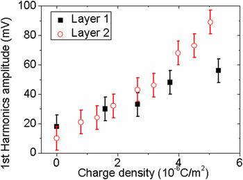
To study how the position of the charge influences the output signal, the position of the charge layer was changed and the output signals were compared. This was fulfilled by using two dielectric films with different thicknesses. Similarly, as also seen in Fig. 3, two dielectric films of 0.01 and 0.05 mm thickness were used. In Fig. 6, the charged layer is 50 μm distant from the grounded electrode. The overall thickness of the dielectric film was fixed at 150 μm. With the two different configurations, the first harmonic amplitude from the piezo sensor as a function of the charge on the layer was measured. Here, the charge is not only dependent on the charging voltage U 0 but also depends on the distance of the layer from the grounded electrodes. Thus, the charge can be calibrated by calculating the capacitance between the floating charge layer and the grounded electrodes. The results are shown in Fig. 6. The first harmonic amplitude of the output shows a similar linear relationship with the charge amount.
Measurements with single charge layer at different locations. Output of first harmonic amplitude with different positions of the charge layer. Layer 1: d 1 = 0.05 mm, d 2 = 0.10 mm; Layer 2: d 1 = 0.10 mm, d 2 = 0.05 mm.

C. Measurements with two floating-charge layers
To simulate a dielectric with two layers of charge, a second copper floating electrode, was added, which is shown as layer 2 in Fig. 3(b). The thickness of the three dielectric films t 1 = t 2 = t 3= 50 μm. To operate this experiment, Layer 1 was first connected to a constant voltage U 1 and then disconnected. Then, Layer 2 was connected to another voltage source U 2 and also disconnected after charging. Thus, both layers carry a fixed amount of charge, depending on the values of U 1 and U 2. By adjusting U 1 and U 2, the amount of charge on Layer1 and Layer 2 can be controlled independently.
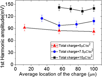
To see how each charge layer affects the output signal, one layer's charge was fixed while the other layer's charge was varied by changing U 1 and/or U 2. The results are shown in Fig. 7. The output signal is more sensitive to the total amount of charge on the two layers, but not as sensitive to how the charge is distributed on Layer 1 and Layer 2. There might be two possible reasons for this. First, if the charge is not far from the center of the film, from Eq. (21), the change of average location of the charge does not affect the output greatly. Second, we simulated two layers of charge using two metal layers. The acoustic wave from the layer farthest from the sensor (Layer 2) will have to pass through more dielectric along with an additional metal-dielectric boundary, which can also affect the result.
Measurement results with two charge layers. The total amount of charge on the two layers is fixed to three different values, and the distribution of charge between the two layers varies. (The charge density on one layer may exceed the total amount of charge because the other layer may carry negative charge.)

D. Lower thickness limit of SEA method
The film thicknesses reported in this work is from 50 to 150 μm. However, the lower thickness limits of this method can be much smaller than this. Theoretically, the tested films can be in the nanometer scale. However, when the films are thinner, the signal will be smaller, based on Eq. (21) and assuming the charge density is not changed. Thus, a much thinner film can be measured with a more sensitive pressure sensor.
V. CONCLUSION
The SEA method can be used to measure the amount of charge inside a dielectric film. The amount of charge is determined by extracting the first harmonic amplitude from the acoustic response signal. Based on the theory, the first harmonic amplitude of the output is proportional to the average charge density (or total charge amount) and also has a dependence on the average position of the charge. However, in the experiment, the output is more sensitive to the average charge density rather than the location and distribution of the charge. Compared to the pulsed acoustic method, the SEA method is much easier to operate; it offers an alternative way to evaluate the charge amount inside a dielectric film and, if the excitation frequency is varied, it offers the ability to find the transfer function of the system in a straightforward manner.
ACKNOWLEDGMENTS
This work was supported by the National Science Foundation under Grant No. CBET-1066231 and by the Semiconductor Research Corporation under Contract No. 2012-KJ-2359.