2.1 Relational event models: an overview

Relational event models build on survival analysis and use network dependencies in event sequences to estimate which factor expedite event occurrence. A sequence of events represent micro-steps in a dynamic network and consist of a sender node, a target node and exact or ordinal timing. REMs are used to estimate the effect of past network events on future events whilst controlling for exogenous factors. Since all network changes in the model are reflected in the event sequence, these events can be considered conditionally independent of one another and can therefore be analyzed using conventional regression models (Butts Reference Butts2008; Lerner et al. Reference Lerner, Indlekofer, Nick and Brandes2013).

The general idea behind REMs is that event occurrence is modeled using a piecewise constant hazard model (Butts Reference Butts2008). The likelihood that an event or a number of events $n_{ij}(t)$ take place on a dyad $(i,j)$ within the time interval $t$ is given by the hazard rate $\unicode[STIX]{x1D706}_{ij}(t)$ . The hazard rate is then multiplied by the survival function $\exp (-\unicode[STIX]{x1D706}_{ij}(t))$ , which captures all events that could have occurred at time $t$ yet did not (see Butts Reference Butts2008, 161–3 and Lerner et al. Reference Lerner, Bussmann, Snijders and Brandes2013, 18–9):

(1) $$\begin{eqnarray}p(n_{ij}(t))=\frac{\unicode[STIX]{x1D706}_{ij}(t)^{n_{ij}(t)}\exp \left(-\unicode[STIX]{x1D706}_{ij}(t)\right)}{n_{ij}(t)!}.\end{eqnarray}$$

The probability density of the event sequence multiplies the likelihood over all dyads and all time intervals $t_{1}$ to $t_{N}$ .

(2) $$\begin{eqnarray}f_{\unicode[STIX]{x1D706}}\left(E,\unicode[STIX]{x1D703}^{\unicode[STIX]{x1D706}}\right)=\mathop{\prod }_{t=t_{1}}^{t_{N}}\left(\mathop{\prod }_{ij\in D_{act}(t)}\frac{\unicode[STIX]{x1D706}_{ij}(t)^{n_{ij}(t)}}{n_{ij}(t)!}\right)\exp \left(-\mathop{\sum }_{ij\in D}\unicode[STIX]{x1D706}_{ij}(t)\right),\end{eqnarray}$$

where $D_{act}(t)$ represents all dyads in which at least one event occurred over the entire event sequence and $D$ represents all possible events that could have potentially occurred (Lerner et al. Reference Lerner, Bussmann, Snijders and Brandes2013, 18–9). For a more detailed derivation and specification of the probability density function, see Lerner et al. (Reference Lerner, Bussmann, Snijders and Brandes2013, 14–9) or Butts (Reference Butts2008, 161–3).

Figure 1.

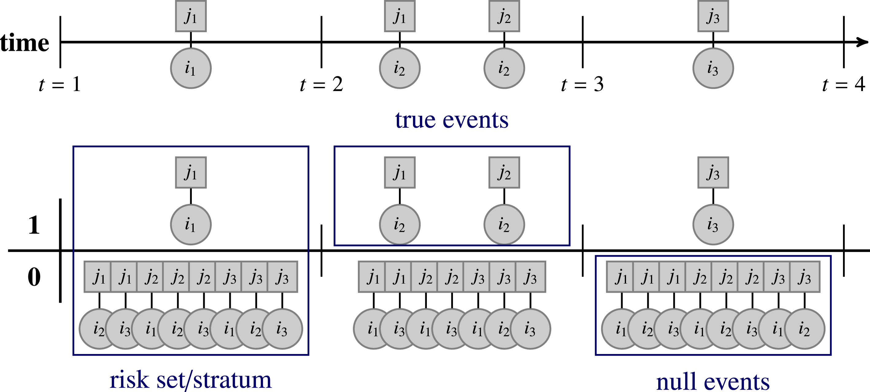
Stratified Cox regression set up of a discrete-time event sequence. For each event in the event sequence a risk set of all events that could possibly occur at said time $t$ is defined which forms a stratum. The risk set consists of true events, i.e., events that took place at time $t$ , and null events, i.e., events that did not occur at time $t$ . Examples of risk sets, true events and null events are encircled in blue in the figure.

A stratified Cox regression can be used to model the effects endogenous or exogenous variables have on the hazard rate. Figure 1 illustrates the basic idea behind a stratified Cox regression with constant event times. For each distinct point in time the risk set $D$ is formed, consisting of events that occurred at said time point (true events) and event that did not occur (null events).

The main distinction of REMs to conventional survival models is the endogenous network statistics that are used as independent variables to explain (together with other exogenous factors) event occurrence. These endogenous statistics are calculated as time-varying covariates and capture network patterns that are assumed to expedite event occurrence, i.e., they capture how nodes react to changes in their surrounding network.

Endogenous network statistics are calculated for each true and null event over all past events $E=(e_{1},e_{2},\ldots ,e_{n})$ :

(3) $$\begin{eqnarray}G_{t}=G_{t}(E)=(A,B,w_{t}).\end{eqnarray}$$

A weight function $w_{t}$ can be applied to each past event in order to account for memory loss or the general passage of time (Brandes, Lerner, and Snijders Reference Brandes, Lerner and Snijders2009; Lerner et al. Reference Lerner, Bussmann, Snijders and Brandes2013). For instance, the weight function can use an exponential decay so that more recent events are given more weight than more distant events:

(4) $$\begin{eqnarray}w_{t}(i,j)=\mathop{\sum }_{\substack{ e:a_{e}=i,b_{e}=j, \\ t_{e}<=t}}|w_{e}|e^{-(t-t_{e})\left(\frac{\ln (2)}{T_{1/2}}\right)}\frac{\ln (2)}{T_{1/2}}.\end{eqnarray}$$

The weight function $w_{t}$ sums over all past events $e$ , i.e., events that occurred before the current time $t$ and that consist of a sender $i$ (with $a_{e}$ denoting this specific sender involved in an event $e$ ; $i=a_{e}\in A$ ), a target $j$ ( $j=b_{e}\in B$ ) and occurred at time $t_{e}$ ; $w_{e}$ can be included if events are not considered of equal importance and weighted accordingly. Each past event is exponentially weighted by how long ago the event took place ( $t-t_{e}$ ). The half-life parameter $T_{1/2}$ can be used to adjust the down-weighting of the event, with a larger half-life indicating slower rate of decay and therefore giving less weight to the passage of time (Lerner et al. Reference Lerner, Bussmann, Snijders and Brandes2013).

The weight function $w_{t}$ is used in the calculation of endogenous network statistics $l$ , such as sender activity for instance:

(5) $$\begin{eqnarray}\text{l}_{\text{senderActivity}}(G_{t},a,b)=\mathop{\sum }_{j\in B}w_{t}(a,j).\end{eqnarray}$$

The statistic captures to what extent actor $a$ ties to $b$ at time $t$ because $a$ has been active in the (recent) past on different target nodes $j$ .

Different network configurations, such as triadic or four-cycle closure, homophily effects or endogenous similarities, can be translated into the REM framework and adapted to heed the timing of events.

However, model specification can pose a challenge for two distinct reasons. First, operationalization of theory-based mechanisms into endogenous network statistics is not always straightforward (see for instance Leifeld and Brandenberger Reference Leifeld and Brandenberger2019) and is further complicated by the addition of the temporal dependencies, which add another layer of complexity. Second, if these operationalization problems can be overcome, it is difficult to know from the estimated models themselves, whether network dependencies have been captured well by the endogenous network statistics included in the model. Butts (Reference Butts2008) stresses the importance of capturing all network dependencies among the events in the event sequence in the form of endogenous network statistics to receive unbiased estimates. If some endogenous network statistics are neglected, other statistics may be over- or underestimated and lead to faulty interpretations of results.

One way to overcome these challenges of model specification is through appropriate goodness of fit tests. The next section addresses shortcomings of conventional goodness of fit statistics and proposes an alternative way of assessing fit via simulated event sequences. These goodness of fit tests from simulated sequences can be used to assess whether the specified model terms capture the network characteristics adequately. And more importantly, these goodness of fit tests can be used to figure out which network dependencies are currently not modeled sufficiently so that they can be included in future models and prevent biased estimates.

2.2 REMs and goodness of fit statistics

REMs only produce unbiased estimates if they fully capture the endogenous network formation processes (Butts Reference Butts2008, 168). In other words, if a dynamic network is theorized to include some form of network closure, an appropriate model term capturing this closure needs to be controlled for to ensure other model terms are not over- or underestimated. To fulfill this requirement for complete capture of endogenous processes in the event sequence, goodness of fit statistics are helpful in guiding model term selection and model specification.

One way of examining model fit is to calculate receiver operating characteristic (ROC) curves or PR curves (Davis and Goadrich Reference Davis and Goadrich2006). While these tools are helpful for evaluating cross-sectional network analyses or dynamic network analyses using snapshots of networks over time (Leifeld, Cranmer, and Desmarais Reference Leifeld, Cranmer and Desmarais2018), they do not fare well with REMs. The problem lies in the calculation of the precision, or positive predictive value. Precision is defined as the fraction of selected events from the risk set that actually occurred in the specified stratum (i.e., true positives divided by the sum of true positives and false positives). Since each stratum only represents one micro-step in the dynamic network, the precision value may be too restrictive. Take for instance a dynamic model where sender activity is one of the dominant traits. At time $t=1$ , sender $i_{1}$ engages in target $j_{1}$ . At time $t=2$ , sender $i_{1}$ then engages in target $j_{2}$ . At time $t=3$ , sender $i_{1}$ then engage in target $j_{3}$ . The precision value calculates the power of the model by checking how many events can be correctly identified per stratum, i.e., per unit of time. Since both events are relatively similar and close together in time, the precision value can be low because its calculation does not allow for small temporal errors, i.e., selecting ( $i_{1}$ , $j_{3}$ ) at time $t=2$ instead of ( $i_{1}$ , $j_{2}$ ).

Furthermore, PR and ROC curves do not give any indication on whether network dependencies have been captured in a satisfactory way. This holds true for other forms of fit parameters, such as the Bayesian information criterion (BIC). Both goodness of fit statistics can give no information on whether endogenous patterns in the data are sufficiently controlled for. Additional goodness of fit statistics for REMs are necessary to check network dependencies, the timing of events as well as predictive power of the model.

2.3 Predicting subsequent events

One way of examining model fit is to create artificial event sequences based on a specified REM. The approach mirrors the goodness of fit tests used in Exponential Random Graph Models (and temporal extensions thereof; see for instance Hunter, Goodreau, and Handcock Reference Hunter, Goodreau and Handcock2008 or Hunter et al. Reference Hunter, Handcock, Butts, Goodreau and Morris2008) in the sense that new event sequences are simulated and compared to the original event sequence. Comparisons of the timing of events as well as whether or not other network dependencies have been captured well can be tested using such simulated sequences. For the sake of clarity, Table 1 disentangles nomenclature for true and null events for the original and the simulated sequences. Simulated true events refer to newly predicted events in the simulation and original true events refer to events in the original data set.

Table 1.

Terminology for simulated and original events.

A simple procedure is proposed here to simulate new relational event sequences (see Algorithm 1) and each step is explained in more details below. The proposed procedure can be used for continuous-time (or exact-time) event sequences as well as for ordinal-time event sequences.

Step 1: Prediction setup. Relational events can be predicted either as within-sample or out-of-sample predictions. For within-sample predictions, a REM is fitted over the full range of the event sequence. For the prediction the original event sequence is then cut at a distinct stratum and subsequent events are simulated from there on and are later compared to the subsequent original event sequence. For out-of-sample predictions, a REM is fitted over a portion of the event sequence and new predictions are appended to the fitted portion of the data. The simulated sequences are later compared to the excluded sample.

Step 2: Defining the risk set for the new stratum and calculating endogenous network statistics. In order to predict next events, new strata have to be built. The stratum represents all possible events that can occur at a given point in time. Depending on whether or not the event sequence presents as time-dependent, the strata can be either static (i.e., the same for each prediction round) or dynamic (changing for each prediction round). A dynamic risk set or strata is necessary for event sequences where events can only occur at specific points in time or where events can only occur once over the entire event sequence. For instance, a member of Congress $a$ can only sign their support for a bill $b$ once. This action cannot be repeated and should therefore not be included in the risk set in the following stratum if the event occurred in the present stratum (for an overview over dynamic and static risk set definitions, see Brandenberger Reference Brandenberger2018b).

After the new stratum is defined, endogenous network statistics (and time-varying covariates) need to be calculated. These endogenous statistics depend on all past events, so whenever new events in a stratum are predicted, these simulated true events (i.e., the newly predicted events in the simulation, see Table 1) will subsequently affect all other events as they become part of the network of past events $G_{t}$ .

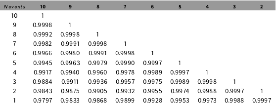
Step 3: Defining the number of events. In order to calculate survivor probabilities, the number of events $d_{i}$ (also known as the number of deaths in survival analysis terms) has to be defined. The overall mean number of events per stratum can be used to define $d_{i}$ or a moving average can be defined to allow for more dynamic event occurrence. It is important to note that over- or underestimating the number of events does not affect the calculation of the survivor probability much (see Table 2 in Section 3).

Step 4: Calculating the baseline hazard for the strata.

The baseline hazard in a Cox model is defined as

(6) $$\begin{eqnarray}{\hat{h}}_{0}(t_{i})=\frac{d_{i}}{\mathop{\sum }_{j,t_{j}\geqslant t_{i}}\exp (x_{j}\hat{\unicode[STIX]{x1D6FD}})},\end{eqnarray}$$

where $d_{i}$ is the number of events that occur at $t_{i}$ for sender $i$ , $x_{j}$ is the covariate vector and $\unicode[STIX]{x1D6FD}$ the estimated coefficients of the model. The baseline hazard is constant for all events in a given stratum and is therefore not relevant for the estimation of the coefficients. It can be used, however, to calculate survivor probabilities (Cox and Oakes Reference Cox and Oakes1984, 107).

Step 5: Calculating the survivor probability for each event in the stratum. The probability of an event surviving to the next point in time is defined as

(7) $$\begin{eqnarray}{\hat{S}}_{i}(t)={\hat{S}}_{0}(t)^{\exp (x_{i}\hat{\unicode[STIX]{x1D6FD}})},\end{eqnarray}$$

where ${\hat{S}}_{0}(t)=\exp (-(\sum _{j,t_{j}\leqslant t}{\hat{h}}_{0}(t_{j})))$ .

This survivor probability reflects the probability that an event does not occur at time $t$ . It is calculated for each event in the stratum and determines whether or not an event is likely to occur or not.

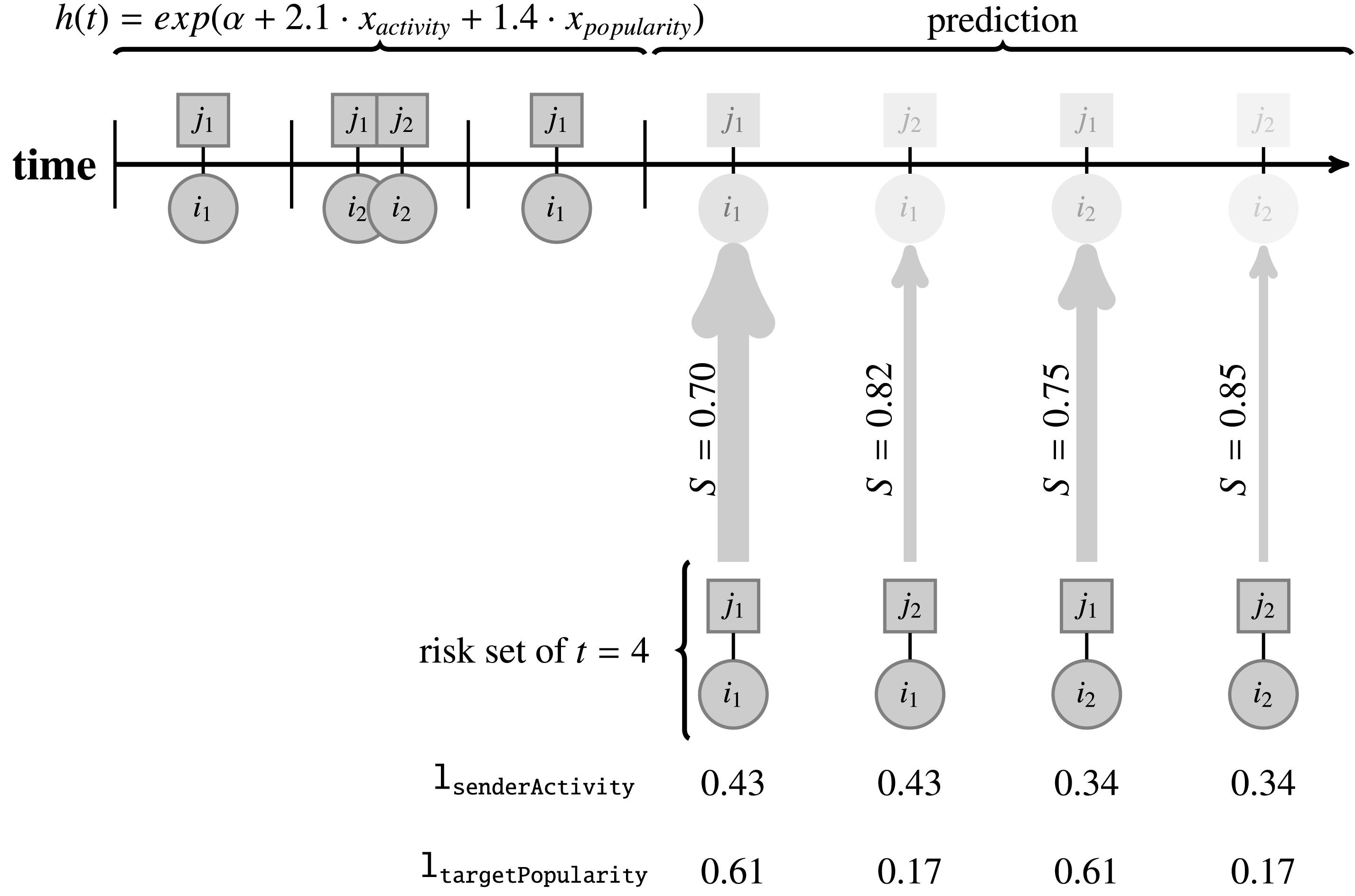
Figure 2 illustrates prediction steps 4, 5, and 6 with a simple example sequence. Assume you have an event sequence with three event days and would like to predict an upcoming event at $t=4$ (for instance to check out-of-sample prediction by holing back the stratum at $t_{4}$ and comparing it to the simulated sequence later). First, the risk set has to be defined for $t=4$ . Here, events can be repeated, so the risk set is defined as broad as possible, with $senders~\times ~targets$ . Next endogenous network statistics are calculated for all events in the new strata (with half-life parameter $T_{1/2}=1$ ). The baseline hazard is calculated using Equation (6). In the example in Figure 2 the baseline hazard with $d_{i}=1$ is ${\hat{h}}_{0}(t_{4})=0.061$ (see Supplementary Information (SI) Online for details on the calculations of this example). The survivor probability can then be calculated for each event in the stratum. The model ( $t=1$ to $t=3$ ) is specified to include sender activity and target popularity. The relational event $(i_{1},j_{1})$ has a high senderActivity and a high targetPopularity. In a model perpetrated positively by sender activity and target popularity, this event is chosen to be the most likely to occur next. Event $(i_{1},j_{1})$ has to lowest survivor probability ${\hat{S}}_{(i_{1},j_{1})}(t_{4})=0.7$ (i.e., a 30% probability of occurring at $t=4$ ).

Figure 2.

Illustration of event prediction at $t=4$ . The risk set for $t=4$ is specified. For each event in the risk set the endogenous network statistics are calculated. Using the specified model, the baseline hazard (with $d_{i}=1$ ) and survivor probabilities are calculated. The event with the lowest survivor probability is most likely to occur next (arrow width and event opacity).

Step 6: Predict new events. New events can be selected by sampling from the stratum and weighting events with their probability to survive to the next time unit. To keep the number of events in check, the sum of all true events should be monitored (see lines 9–11 in Algorithm 1). Since the strata are added to the event sequence, allowing for more than the specified number of events $d_{i}$ can cause the prediction of the next stratum to spin out of control.

Step 7: Append stratum to the event sequence. At the end of each prediction round, the stratum with the newly defined simulated true events is appended to the event sequence and a new prediction cycle starts again. As such, newly simulated events are used to predict subsequent events and so forth. The appended stratum is incorporated into the network of past events $G_{t}$ for the subsequent strata. This ensures that the sequence evolves beyond simple one-shot predictions. Instead, dynamic sequences are simulated.

2.4 Predicting subsequent events from random events

A simulation test is used to check whether the presented procedure for simulating event sequences is feasible. Given a network of 20 unique sender nodes and 30 unique target nodes, a random event sequence is generated using 50 event days. The resultant 30,000 events ( $20\cdot 30\cdot 50$ ) were randomly sampled into true events (i.e., deaths, $d_{i}$ ) and null events. 200 true events are assigned.

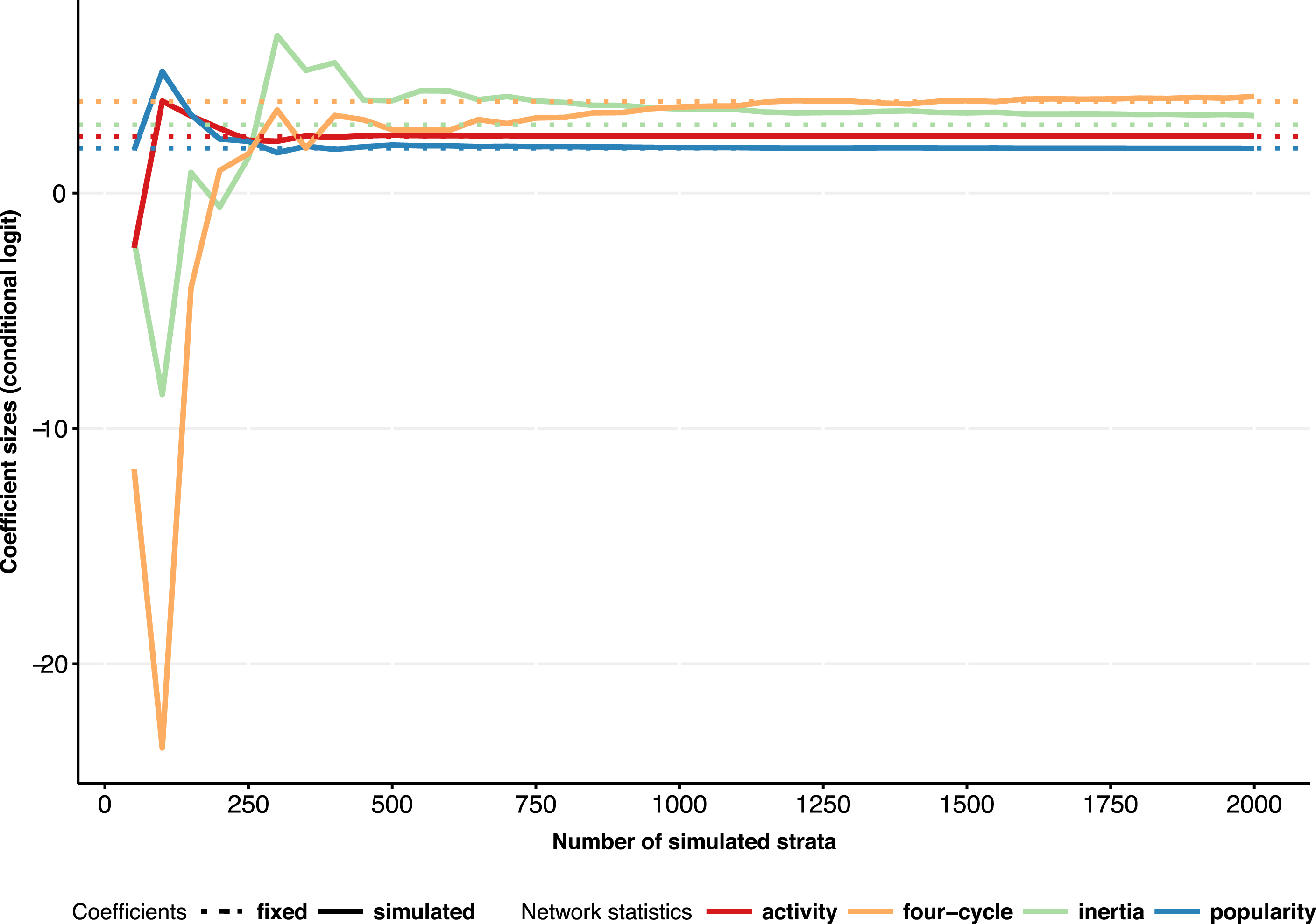
From this baseline, new events were simulated based on an artificially specified REM. The model included inertia, activity, popularity and four-cycle effects. The coefficients for these terms were chosen exogenously. The simulation is run over 1950 strata (resulting in 2000 strata in total). Afterward, conditional logistic regressions were run over different portions of the simulated event sequence to determine whether the coefficients from the simulated sequence reflect the specified coefficients (see SI Online for additional information).

Figure 3 indicates that after around 500 strata, the models start to stabilize around the specified coefficients. The simulation test reveals that the prediction procedure can replicate event sequences based on a specified REM.

Figure 3.

Coefficients from simulated sequences (bold lines) compared to the specified coefficients (dashed lines). The first 50 strata contain 200 random true events. All subsequent events are based on the prediction procedure and coefficients from an artificial Cox model.

3.1 Data and models

The example is based on data from a policy debate. Each event represents a statement a particular organization (sender mode) made and got recorded in the press on how best to resolve the financing problem of the German pension system (Leifeld Reference Leifeld2016). These proposed policy solutions were hand-coded and represent the target mode. The events in the sequence are weighted by a stance dummy, representing agreement for or opposition with a proposed policy solution. The case study as well as the REM are presented in full in Leifeld and Brandenberger (Reference Leifeld and Brandenberger2019).

The data presents an ideal example of the use of REMs to examine micro-dynamics in a social system. Exact- or ordinal-time event sequences offer rich insights into how nodes react to changes in their network. However, they also pose a challenge as theoretical constructs have to be operationalized at the micro-level for fine-grained mechanisms have to be defined to test them. In their paper, Leifeld and Brandenberger (Reference Leifeld and Brandenberger2019) show that REMs can be used to test endogenous coalition formation through policy learning mechanisms. Several policy process theories address the importance of policy learning for coalition formation (see for instance Sabatier and Jenkins-Smith Reference Sabatier and Jenkins-Smith1993); however, none of them offer concrete insights into how learning takes place (i.e., the mechanism behind it). Leifeld and Brandenberger (Reference Leifeld and Brandenberger2019) operationalize learning as closing four-cycles, where policy solutions are gradually picked up by a focal organization if other nodes in the network, with whom the focal organization has shared policy solutions in the past, postulate them. Similarly, organizations learn from their opponents by repeatedly rejecting solutions they advocate. These two endogenous learning effects are tested using the German pension financing debate as a case study.

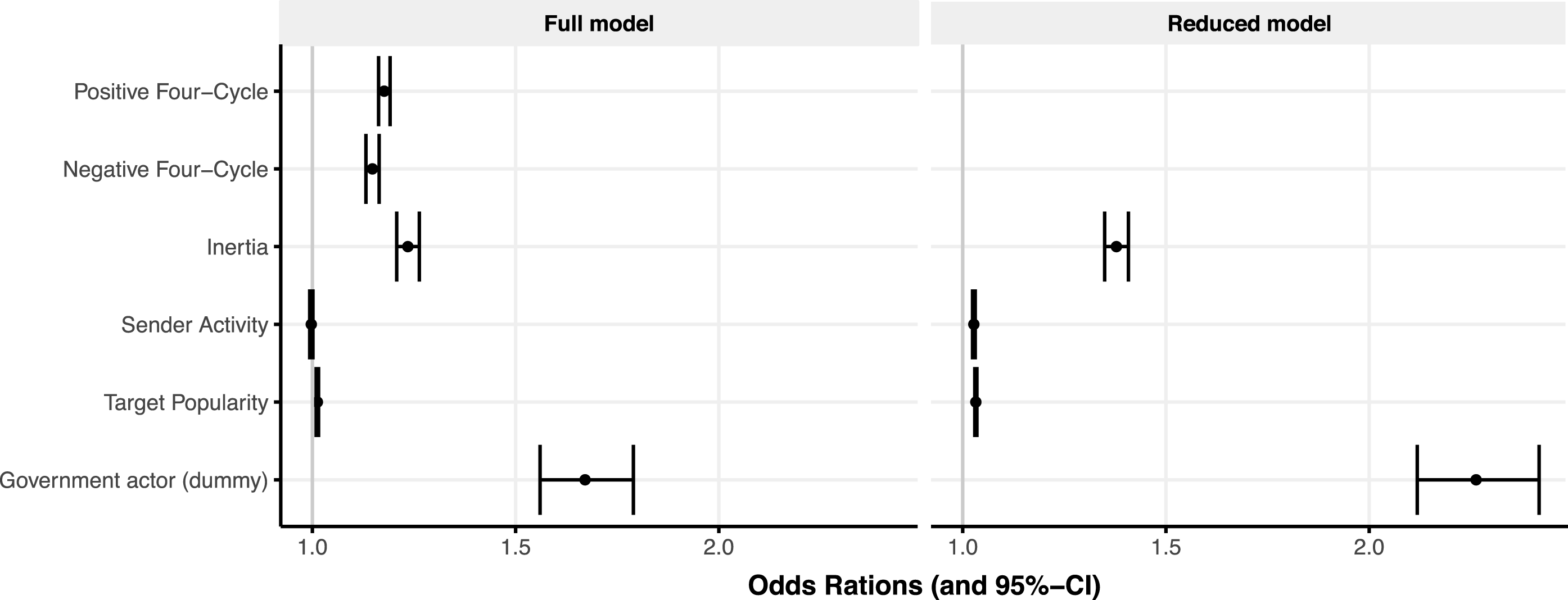
A full model and a reduced model are presented here from which within-sample predictions are made. Figure 4 reports the results of both models. The full model contains four-cycle statistics that represent learning mechanisms in policy debates (for additional details, please refer to Leifeld and Brandenberger Reference Leifeld and Brandenberger2019). The reduced model only contains control variables with inertia, sender activity and target popularity as endogenous network statistics.

Even though the four-cycle learning effects show positive effects in the REM (see Figure 4), it is unclear by how much they improve the predictive fit of the model or if they are even necessary to capture the endogenous process in the debate sequence. For theory-building purposes, the proposed goodness of fit tests can be used to assess the impact of the learning mechanisms in explaining the temporal and network structure of the debate.

The data contains 6,704 statements, made over the course of nine years (1993–2001) and were manually coded from 1,842 newspaper articles using tools from discourse network analysis (Leifeld Reference Leifeld, Victor, Lubell and Montgomery2017). The sender mode contains of 245 organizations and the target node contains 69 policy solutions (for additional information on the data, see Leifeld Reference Leifeld2016).

Table 2.

Correlation matrix of survivor probabilities with different definitions of number of events ( $d_{i}$ ). Survivor probabilities are calculated for the stratum at $t=989$ . The choice of $d_{i}$ does not affect survivor probabilities much. Correlations of survivor probabilities with different baseline hazards are all close to 1. Please refer to the SI Online for further details on the calculation of the correlation matrix.

Figure 4.

Results of the stratified Cox model on event occurrence. Events correspond to political statements organization made during the German pension debate. Endogenous network statistics are used to capture temporal patterns of interactions in the debate. The full model contains four-cycle statistics to capture learning patterns among organizations. (Note: AIC full model $=54219.64$ , AIC reduced model $=55452.81$ . Mc-Fadden $pseudo-R^{2}$ is $0.13$ and $0.11$ for the full model and the reduced model, respectively. Estimations based on 6044 true events and 877,811 null events.)

In order to test the fit of the two models, within-sample predictions were made and compared to the original sequence. 1,000 distinct event sequences were simulated starting at stratum $t=700$ (representing event date March 26, 1999) and ending at stratum $t=800$ (representing event date September 29, 1999).Footnote ² The risk set for the prediction was defined by all sender–target combinations that were voiced throughout the entire debate $D_{act}(t)$ , resulting in a strata containing $1916$ events from which next events were selected based on their survival probability. The number of events $d_{i}$ were set to $d_{i}=8$ based on the average number of events occurring between $t=700$ and $t=800$ (mean number of events per stratum $=7.8$ ). The choice of $d_{i}$ barely affects the calculation of the baseline hazard and by extension the survivor probabilities. Table 2 holds the correlations between survivor probabilities of events in a stratum based on different numbers of events $d_{i}$ . All correlations are close to 1 (see SI Online for additional information). 1,000 event sequences were simulated for both the full model and the reduced model. Additionally 1,000 event sequences were generated based on a random selection of $d_{i}$ events per stratum.

3.2 Temporal prediction error

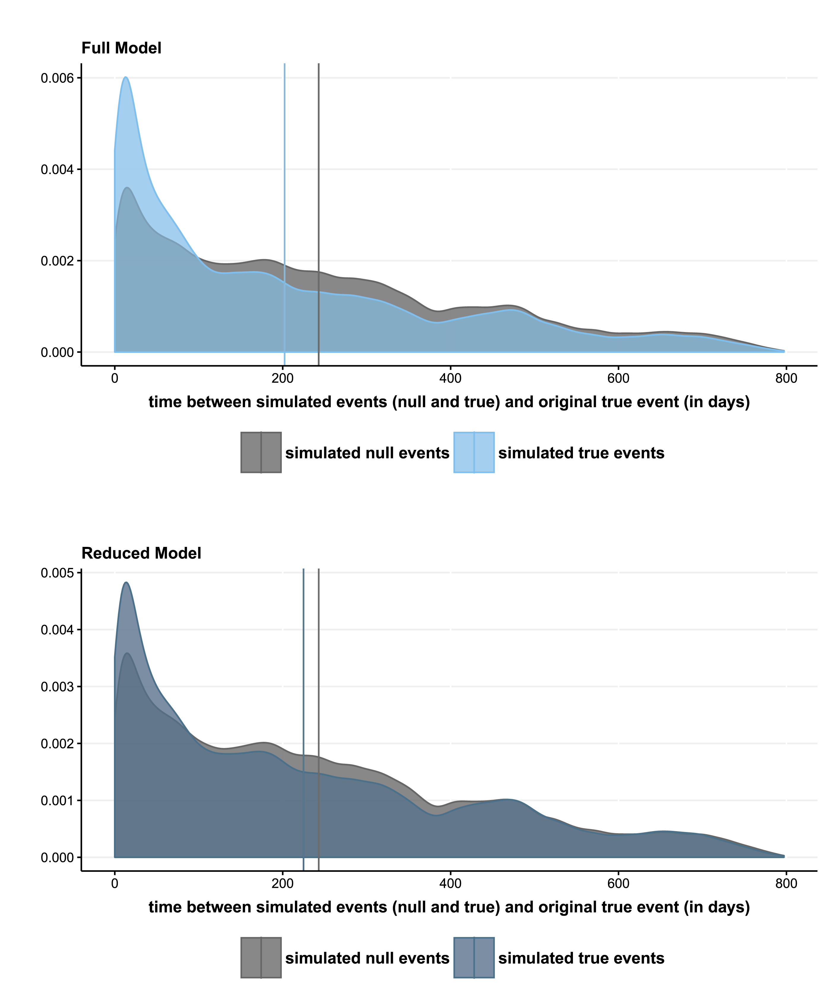
In a first goodness of fit test the timing of simulated events is examined. If the model has predictive power, the simulated true events should be closer to the original true events than the simulated null events. This would indicate that the simulation chooses events to occur next that are more closely related to the temporal position of the original true events.

Figure 5 shows density plots of the time between simulated (null and true) events and original true events, i.e., the temporal prediction error. Comparing the distributions and overall means of the temporal prediction error for simulated true events between the two models reveals by how much the model improves if endogenous four-cycle statistics are included.

Figure 5.

Goodness of fit assessment of the full model through timing of simulated events. The temporal prediction error is calculated by the difference between the original true event and the simulated (true and null) event. For the full model, the mean temporal prediction error for simulated true events is $202.25$ days and $242.85$ days for simulated null events. For the reduced model, the mean temporal prediction error for simulated true events is $224.81$ days and $242.89$ days for simulated null events.

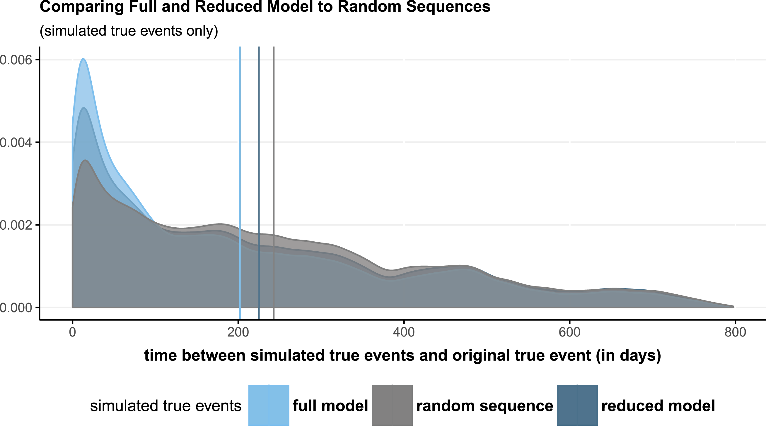
Figure 6 reports the temporal prediction error for simulated true events only (i.e., excluding null events). The mean temporal prediction error for the full model is $202.25$ days. For the reduced model, the error is $224.81$ . Comparing the two distributions and means to the temporal prediction error of fully random sequences allows an assessment of how the models perform compared to a random baseline. The mean temporal prediction error of the random sequence is $242.78$ days and reflects the temporal prediction error of the simulated null events. All in all, the calculations show that four-cycle statistics improve the model drastically.

Figure 6.

Temporal prediction error of simulated true events for the full and reduced models as well as for random sequences. The temporal prediction error is calculated by the difference between the original true event and the simulated true event. Mean temporal prediction error of the full model is $202.25$ days, $224.81$ days for the reduced model and $242.78$ days for the random sequence.

3.3 Precision of event prediction with tolerance

In a second goodness of fit test, the accuracy of simulated events is examined. For each simulated stratum, the simulated true events are compared to the original true events to check if the original true events have been predicted. Matching senders, targets or sender–target combinations can be evaluated. To ensure that the predictions are not judged too restrictively, as is done in the precision measure, a tolerance can be introduced. The tolerance can check whether simulated true events are located within a particular time span.

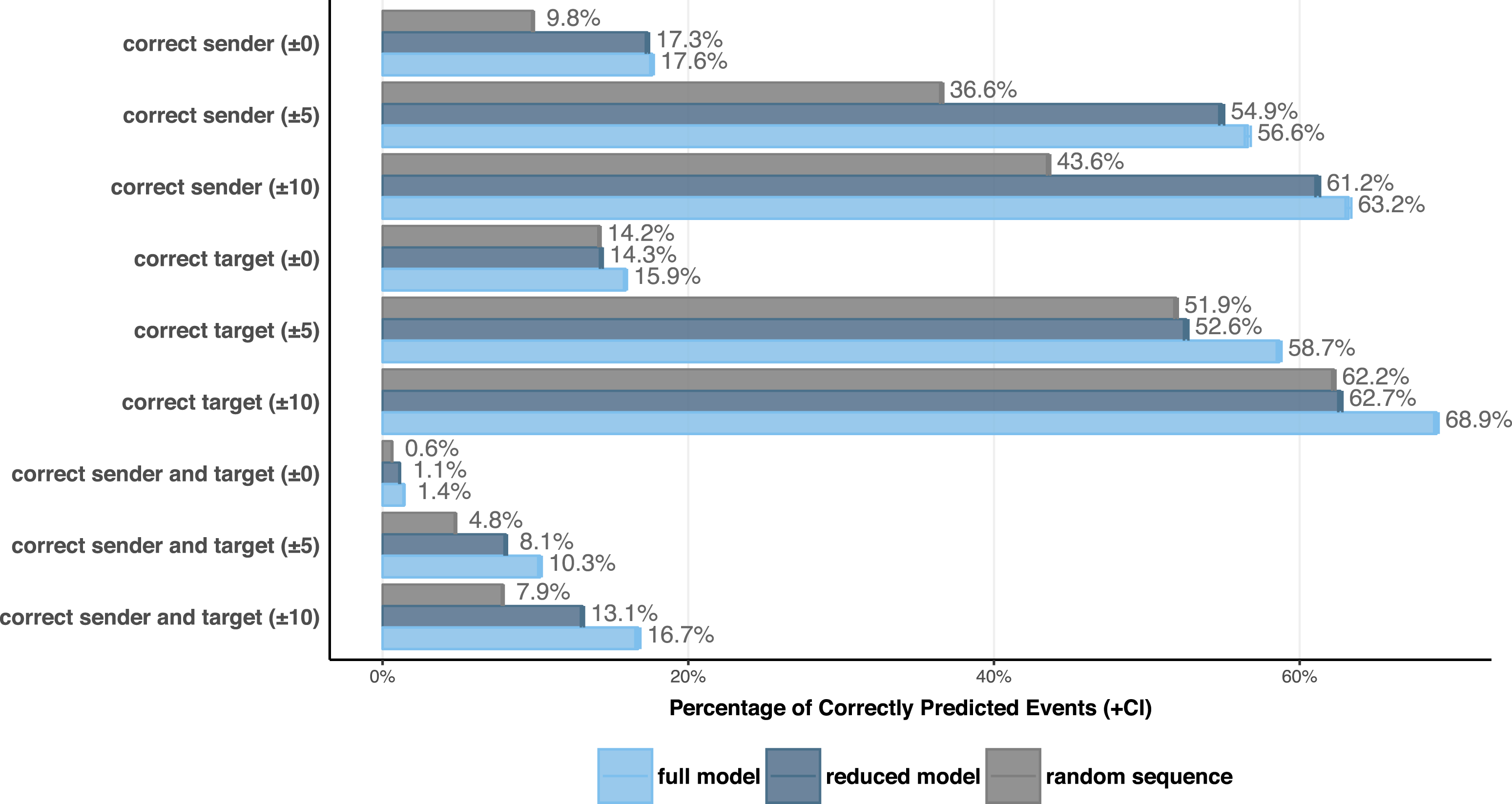
Figure 7 reports the results of the event matching test. Next to exact matching, correct predictions within a tolerance of 5 days and 10 days are reported as well. The comparison to the random sequence is useful if the risk set is made up of conditional events, i.e., events that occurred at least once over the sequence instead of all possible sender–target combinations. The random sequence provides a baseline against which the models can be checked. For instance, the random sequence predicts 10% of all its sender nodes (exact timing). The reduced model increases the matching outcomes to 17.3%. Including four-cycles, however, does not improve prediction of sender nodes much compared to the reduced model (17.6%). If a tolerance of 5 event days is used to evaluate matches, the full model improves slightly over the reduced model. Over 50% of all sender nodes are predicted correctly with the reduced and the full model with a tolerance of 5 event days.

Figure 7.

Goodness of fit assessment through event matching. The bar chart shows by how much the reduced and full models improve the prediction of senders, targets and sender–target combinations vis-à-vis the randomly predicted sequence. Confidence intervals are based on 1,000 simulated sequences.

Looking at the prediction of target nodes shows that the inclusion of the four-cycle statistics slightly increases the correct prediction of target nodes. Even though the full model reaches almost 70% correct target nodes (with a tolerance of 10 event days), it is important to note that the random sequence is able to get 62% of all targets with the same tolerance. A comparison to random sequences is helpful for event sequences where events repeat themselves.

Most importantly, the specified REM should be able to predict both sender and target nodes together, i.e., the full relational event. Prediction success is low for both the reduced and the full model (compared to the random sequence) if exact matches are examined. Increasing the tolerance by 5 days increases prediction by a factor of seven (for the full model). Finding 10% of all events within a 10 day span (plus–minus 5 days) is a remarkable feat, since the risk set contains 1,916 unique events and a total of eight events at the most are chosen for each simulated stratum.

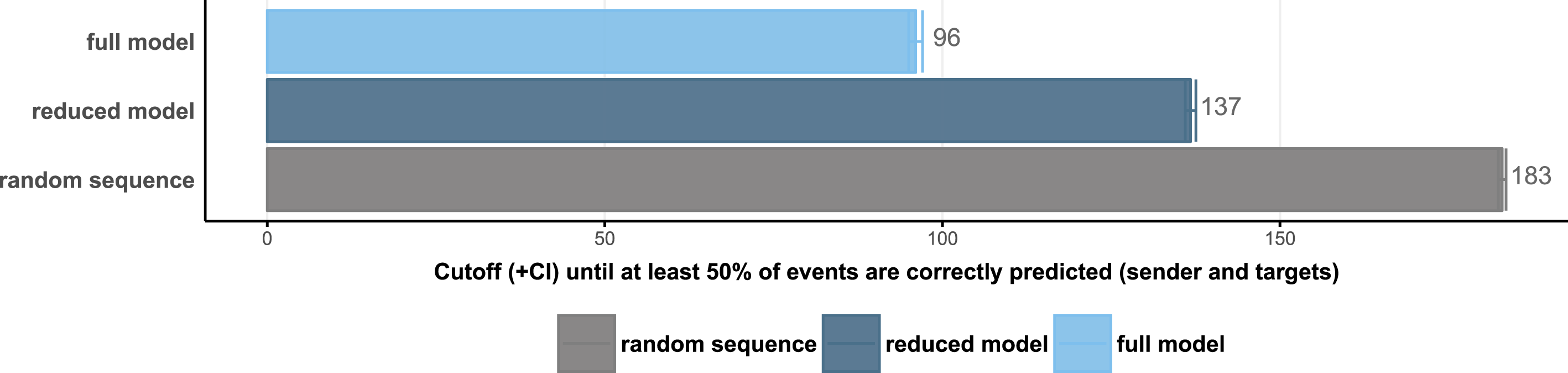
Alternatively, event matching can be used to examine how wide the tolerance has to be set to reach 50% correct prediction of sender–target events (see Figure 8). This is useful to quickly compare different model specifications, as well as models using alternative risk set definitions or half-life parameters in the time-weighting of past events.

Figure 8.

Goodness of fit assessment through event matching. The bar chart shows how large the tolerance has to get until the model reaches 50% correct event (sender–target combinations) predictions. The lower the tolerance, the better the model fit. Confidence intervals are based on 1,000 simulated sequences.

3.4 Checking endogenous network structures

Whilst temporal prediction errors and event matching are useful for comparisons of different model specifications and establishing which model terms should be included in the model, neither can establish if network dependencies have been captured fully, as needed for the REM to estimate unbiased coefficients.

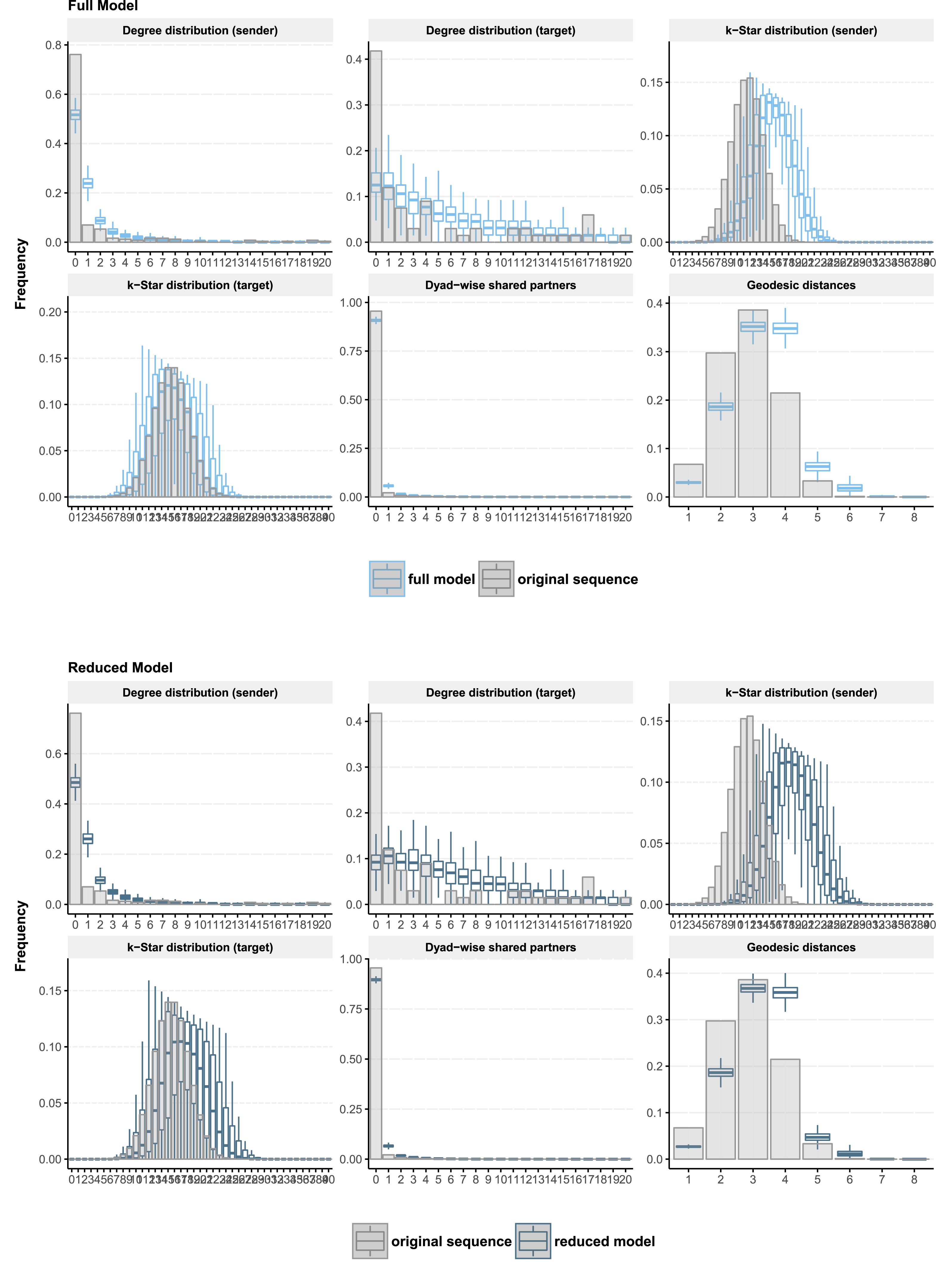
Figure 9 shows network characteristics captured by the simulated sequences compared to the original sequence. The original event sequence and 1,000 simulated sequences are aggregated into a cross-sectional network snapshot (using all events between event days 700 and 800). As is done with other network models when checking fit (Robins, Pattison, and Woolcock Reference Robins, Pattison and Woolcock2005; Hunter et al. Reference Hunter, Handcock, Butts, Goodreau and Morris2008; Cranmer et al. Reference Cranmer, Leifeld, McClurg and Rolfe2017), different network characteristics are calculated based on these snapshots, such as degree distributions (for both modes separately). If the REM is able to capture endogenous processes well, then the simulated sequences should reveal similar network characteristics as the original sequence does. In Figure 9, the degree distributions (for the sender and target mode) of the original event sequence are depicted in a bar chart. Degree distributions are then calculated for the 1,000 simulated sequences and plotted as box plots (to show the variation between the different simulations) on top of the bar chart. Comparing the original and simulated degree distributions shows that the fit is not perfect; yet both models show some congruence with the original degree distributions (with the full model performing slightly better than the reduced model; see left two panels in the top row of Figure 9). Adding the four-cycle statistics helped align the degree distributions of both modes. The k-star distribution of the sender mode is slightly overestimated by the REM, though less so in the full model. The k-star distribution of the target mode as well as dyad-wise shared partner distributions and geodesic distances are captured well in the full model and slightly less so in the reduced model. All in all, the model-based simulations are able to capture network properties fairly well.

Figure 9.

Goodness of fit assessment through comparison of network characteristics. The bar chart represents the distributions from the aggregated network of events between event day 700 and 800 of the original event sequence. The box plot corresponds to the distributions captured in the model-based simulations. The full model captures degree distributions fairly well, slightly overestimates k-star distribution of the sender mode and yields passable results for k-star distributions of the target mode, dyad-wise shared partner and geodesic distance distributions.