

Introduction
The stability of a population is a complex phenomenon, requiring at least two parameters, population variability and persistence, to encompass the concept (Grimm and Wissel Reference Grimm and Wissel1997; Lamb and MacKay Reference Lamb and MacKay2010; Lamb et al. Reference Lamb, MacKay and Alyokhin2011). Population variability reflects the ups and downs in abundance of a population from year to year, estimated here by PV, a proportion between 0 and 1 (Heath Reference Heath2006). A species that fluctuates widely in abundance has a high PV, and is perceived to be less stable than one that fluctuates less widely. A species that frequently disappears from a habitat also is perceived to have a less stable population than one that is more persistent, even if both fluctuate similarly. Persistence is defined here as the probability that a species occurs in a particular year at a location, estimated as the proportion of years in a time series of annual abundance that the species is present (Lamb and MacKay Reference Lamb and MacKay2010).
The stability of relatively few insect populations has been quantified using these metrics, because long time series of population abundance are required, and because robust methods to quantify the parameters, particularly population variability, have only recently been developed. The eight populations of four species of aphids (Hemiptera: Aphididae) for which stability has been quantified have high PV and high persistence (Lamb and MacKay Reference Lamb and MacKay2010; Lamb et al. Reference Lamb, MacKay and Alyokhin2011). These species are free-living herbivores of herbaceous plants, representing some, but by no means all of the variation in life history exhibited by aphid populations.
Three populations of the aphid Baizongia pistaciae (Linnaeus) were sampled in Israel for 20 years on its primary host, the tree Pistacia palaestina Boissier (Anachardiaceae), to diagnose underlying causes of temporal changes in abundance (Wool Reference Wool2002). Only weak correlations with weather and “no convincing evidence of self regulation (density dependence)” were detected (Wool Reference Wool2002). Wool's (Reference Wool2002) study provides time series of abundance that are used here to assess the stability of populations of an aphid with a more permanent host than, and a life history that differs from, the aphids so far investigated. Baizongia pistaciae has a 2-year life cycle, alternating between a primary host tree and a secondary host, a grass (Graminae) (Wool Reference Wool1990, Reference Wool2002, Reference Wool2004). The aphid passes through three generations in one summer within characteristic large galls on Pistacia. As summer ends, winged females migrate to the soil and produce larvae that are free-living and feed on the roots of a grass. Their offspring and subsequent asexual generations continue feeding on grass roots through the winter and following summer before migrating back to Pistacia the next autumn. These asexual migrants produce a single sexual generation on Pistacia. A sexual female lays a single egg that overwinters and the parthenogenetic female larva that hatches the following spring initiates a gall. This 2-year life history results in two cohorts that form galls on the trees in alternate years. The cohorts probably have little opportunity to mix, but the extent of genetic exchange between cohorts is not known.
Pistacia trees can be long-lived and often grow in close proximity to the secondary grass host (Martinez et al. Reference Martinez, Mokady and Wool2005). Therefore, this tree–grass system is a more permanent habitat at a particular location than many herbaceous plants, particularly crops. We expected the longevity of its primary host would stabilise populations of B. pistaciae. We also expected the galling habit of B. pistaciae would stabilise populations by protecting them from fluctuating levels of predation and extremes of weather (Wool Reference Wool2002; Martinez et al. Reference Martinez, Mokady and Wool2005), more so than is the case for free-living aphids feeding on herbaceous foliage during summer. Furthermore, we expected populations of B. pistaciae, a native aphid, to be more stable than those of introduced aphids (Lamb et al. Reference Lamb, MacKay and Alyokhin2011). The annual abundances of galls (Wool Reference Wool2002) are used here to estimate the stability of B. pistaciae and compare its stability with that of free-living native and introduced aphids on herbaceous plants (Lamb and MacKay Reference Lamb and MacKay2010; Lamb et al. Reference Lamb, MacKay and Alyokhin2011).
The data on the abundance of B. pistaciae (Wool Reference Wool2002) were collected for two cohorts, from three populations of marked trees, and over many sexual cycles, which provides replication within subpopulations (the local habitat), among subpopulations (individual trees), and among populations. This replication allowed us also to examine hypotheses proposed previously to explain population stability, hypotheses that are more general than those related to the specific life history traits of B. pistaciae, as follows: stability is a function of average population abundance, particularly that low abundance contributes to low persistence (Schoener and Spiller Reference Schoener and Spiller1987) and persistence declines as population variability increases (Inchausti and Halley Reference Inchausti and Halley2003); more time leads to more population variability (Lawton Reference Lawton1988; Pimm and Redfearn Reference Pimm and Redfearn1988; Inchausti and Halley Reference Inchausti and Halley2002); stability increases with spatial scale (Connell and Sousa Reference Connell and Sousa1983); stability is a species trait (Taylor and Woiwod Reference Taylor and Woiwod1980; Lamb and MacKay Reference Lamb and MacKay2010; Lamb et al. Reference Lamb, MacKay and Alyokhin2011).
Materials and methods
The annual abundance of B. pistaciae was estimated by counting galls on individual marked trees each winter at three locations from 1979 to 1998 (Wool Reference Wool2002). The galls are large, long-lasting, and easily counted when trees shed their leaves. Trees were sampled at Mount Carmel in the north of Israel (seven trees for 20 years), at Beit Guvrin in the southeast (six trees for 19 years), and at Tel Aviv in the southwest (24 trees for 17 years); site names are abbreviated to Carmel, Guvrin, and Tel Aviv and used to identify aphid populations. Other trees sampled for shorter periods were excluded from this study to allow consistent comparisons over similar time intervals. The temporal changes in abundance of the aphid, and the characteristics and precise locations of the populations are described by Wool (Reference Wool2002) and references therein.
The galls on a tree were considered to belong to even-year and odd-year cohorts, because of the 2-year life cycle of the aphid. The cohorts were analysed separately, providing time series of 8–10 cycles over the 17–20 years, and replicate subpopulations on individual trees to assess the effect of local habitat on abundance and stability. The three population scales were: subpopulation, the galls on an individual tree (“patch” in Wool Reference Wool2002); population, a group of trees at one location; and region, pooled data for three populations. For B. pistaciae, dispersal of more than 100 m between local tree–grass habitats is limited and longer-distance dispersal between locations is less likely, justifying the conclusion that an individual tree and surrounding grass is “the smallest area in the landscape that sustains a genetically differentiated subpopulation” (Martinez et al. Reference Martinez, Mokady and Wool2005). The estimates of abundance each year for the three spatial scales were calculated as follows: subpopulation – the number of galls on an individual tree; population – the total number of galls on sampled trees at a location divided by the number of trees; region – the average of the three population-scale estimates, which assured that each population estimate contributed equally to the regional estimate although the number of trees sampled differed among populations.
Three population parameters were considered: abundance, population variability, and persistence. Abundance was estimated as described above. Population variability was estimated by the metric PV, the average of the differences for all pairs of abundance in a time series, with each difference divided by the larger abundance of the pair, assuring the index is a proportion between 0 and 1 (Heath Reference Heath2006). Persistence was estimated as the proportion of 2-year cycles in which galls were present: for example, if galls of the even-year cohort were found in 9 of 10 years, persistence was 0.9.
Sources of variation in abundance were analysed by two-way and three-way analyses of variance on ln-transformed or square-root-transformed data to assure normality (SYSTAT 2009). The variance in abundance (and related estimates of variability) estimated from year-to-year fluctuations, which assumes annual abundance is normally distributed and independent from year to year, was not considered to be a valid estimate of population variability (Heath Reference Heath2006; Lamb and MacKay Reference Lamb and MacKay2010; Lamb et al. Reference Lamb, MacKay and Alyokhin2011). Population variability was assumed to be normally distributed because each PV is a mean of many differences (Heath Reference Heath2006). PV was analysed as for abundance, but without transformation. Persistence values were proportions based on relatively small samples (n = 8–10 years) and were between 0.8 and 1.0 for many subpopulations. Therefore, persistence was not subject to analysis of variance. Relationships between population parameters were assessed using Pearson product-moment correlation or linear regression (SYSTAT 2009). Correlation analyses also were used to assess the similarity of population parameters between the cohorts inhabiting trees in alternate years.
Results
Variation in gall abundance
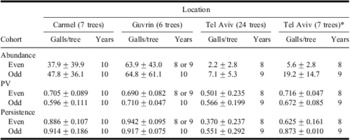
On individual trees, galls were most abundant at Guvrin, with a mean of 64 galls per tree, compared with 43 at Carmel, and five at Tel Aviv (Table 1). The difference between Carmel and Guvrin was detected in analysis of variance of ln-transformed gall abundance, with variance partitioned among locations, cohorts, years within cohorts, and subpopulations within location (F = 5.2, df = 1, 218, P = 0.024). At Tel Aviv, some trees were often free of galls, and the distribution was not normalised by ln-transformation. The difference between Tel Aviv and the other two locations was detected by analysis of variance of untransformed annual mean gall abundance for subpopulations at a location, using a General Linear Model which partitioned variance between the cohorts and among locations (F = 10.2, df = 2, 48, P < 0.001).
Population parameters and standard deviations (±1 SD, n = the number of trees) of Baizongia pistaciae galls on individual Pistacia trees (subpopulation scale) from the even-year and odd-year cohorts of a 2-year life cycle at three locations in Israel.

The parameters are: abundance, the mean number of galls on a tree over years; population variability estimated by PV (see “Materials and methods”); and persistence, the proportion of years galls were present on a tree.
*All subpopulations (trees) at Tel Aviv with persistence ≥0.5.
Gall abundance differed among subpopulations at each location, and between the even-year and odd-year cohorts at Carmel and Tel Aviv although not at Guvrin (Table 1). These differences confirmed the validity of treating the galls on different trees as distinct subpopulations, and considering even-year and odd-year cohorts separately. Differences in abundance among subpopulations and between cohorts were detected in two-way analyses of variance for each location, as follows: Carmel, ln-transformed data for subpopulations (F = 8.4, df = 6, 126, P < 0.001) and cohorts (F = 4.6, df = 1, 126, P = 0.034, nonsignificant interaction); Guvrin, ln-transformed data for subpopulations (F = 3.9, df = 5, 98, P < 0.003) but not cohorts (F = 0.014, df = 1, 98, P = 0.906, nonsignificant interaction); and Tel Aviv, square-root-transformed data for subpopulations (F = 10.8, df = 23, 336, P < 0.001) and cohorts (F = 42.4, df = 1, 336, P < 0.001, significant interaction).
Variation in population stability
Persistence was near 0.9 for both cohorts at Carmel and Guvrin, but low for most of the 24 subpopulations at Tel Aviv (Table 1). PV for subpopulations ranged from 0.50 to 0.71, on average, for the two cohorts and three populations, with PV lowest for both cohorts at Tel Aviv (Table 1). Analysis of variance of PV using a General Linear Model detected differences among locations (F = 4.2, df = 2, 68, P = 0.020), but not between cohorts within location (F = 1.3, df = 3, 68, P = 0.299). When the analysis was repeated excluding data from Tel Aviv where abundance was low, no difference in PV was detected between Carmel and Guvrin (F = 0.83, df = 1, 22, P = 0.372) or between cohorts within location (F = 2.2, df = 2, 22, P = 0.135).
All three population parameters for the 24 subpopulations at Tel Aviv differed from those at the other two locations and therefore variation among subpopulations was examined separately at the three locations. PV differed among subpopulations at Carmel and Guvrin but not at Tel Aviv, and PV was lower for the odd-year than the even-year cohort at Carmel, but not at Guvrin or Tel Aviv (Table 1). These differences were detected in two-way analyses of variance, as follows: Carmel, for subpopulations (F = 21.5, df = 6, 6, P = 0.001) and cohorts (F = 46.2, df = 1, 6, P < 0.001); Guvrin, for subpopulations (F = 10.0, df = 5, 5, P = 0.012) and cohorts (F = 0.02, df = 1, 5, P = 0.893); and Tel Aviv for subpopulations (F = 1.59, df = 21, 21, P = 0.149) and cohorts (F = 2.2, df = 1, 21, P = 0.152).
Relationships among population parameters
Although the average abundance of galls on individual trees varied by as much as an order of magnitude among locations and also varied between the cohorts at two locations, PV was relatively uniform (Table 1). Mean persistence, however, tended to be high when gall abundance and PV were high (Table 1). These relationships were detected by estimating Pearson correlation coefficients: PV versus abundance (R = 0.795, n = 6, P > 0.05); persistence versus abundance (R = 0.935, n = 6, P = 0.006); persistence versus PV (R = 0.864, n = 6, P = 0.026).
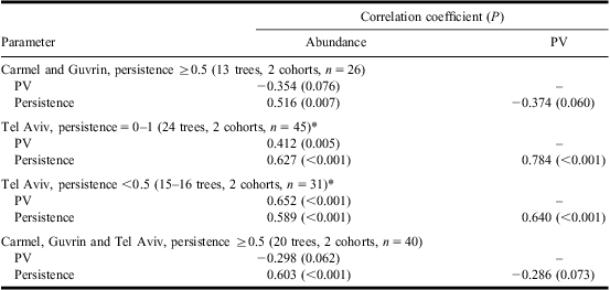
When the relationships among population parameters were examined for individual subpopulations instead of means for subpopulations at a location, more complex patterns emerged. For the 13 subpopulations at Carmel and Guvrin the relationships between gall abundance and PV and between PV and persistence were weak and negative (Table 2), contrary to the strong positive correlations for populations described above. The relationship between abundance and persistence remained positive (Table 2), as expected from the mean values (Table 1). For the 24 subpopulations at Tel Aviv, however, positive relationships were detected among all three parameters (Table 2).
Pearson correlation coefficients, with probability that the coefficient = 0 in parentheses (P), comparing population parameters for 8–10 cycles of Baizongia pistaciae galls from the even-year and odd-year cohorts on individual Pistacia trees in Israel.
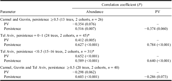
The parameters are: abundance, the mean number of galls on a tree over years; population variability estimated by PV (see “Materials and methods”); and persistence, the proportion of years galls were present on a tree. Estimates were made for: pooled data for subpopulations (trees) at Carmel and Guvrin with high abundance and persistence ≥0.5; at Tel Aviv with low abundance, first for all subpopulations; then for subpopulations with persistence <0.5; and then for subpopulations from three locations with persistence ≥0.5.
*A cohort on a tree with 0 galls in all years was excluded.
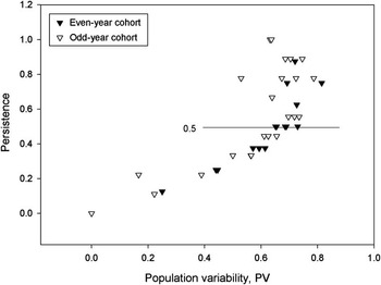
The contrast between the relationships among population parameters at Carmel and Guvrin, on the one hand, and Tel Aviv, on the other, was clarified by considering the relationships between PV and persistence at Tel Aviv in detail (Fig. 1). Persistence increased with PV up to a persistence of 0.5 (R = 0.640, n = 31, P < 0.001; Pearson correlation), but not above 0.5 (R = −0.092, n = 14, P = 0.754). The relationship between PV and abundance at Tel Aviv also disappeared when persistence was ≥0.5 (R = 0.207, n = 14, P = 0.478). When only subpopulations with low gall persistence were considered at Tel Aviv, all relationships between population parameters were positive (Table 2). When only subpopulations with high persistence were considered from all three locations, two of the relationships were negative and weak, and the only significant relationship was between abundance and persistence (Table 2). When half or more of the estimates of abundance in a time series were 0, PV and persistence decreased in proportion to the increased number of 0-values, assuring positive correlations among them. We conclude these positive correlations for low-persistence subpopulations were a numerical consequence of the large number of 0-values that occurred when persistence was near 0.1, rather than meaningful ecological relationships.
Relationship between persistence (proportion of years galls are present) and population variability (PV, defined in “Materials and methods”) of Baizongia pistaciae galls, from even-year and odd-year cohorts, on 24 Pistacia trees at Tel Aviv, Israel.

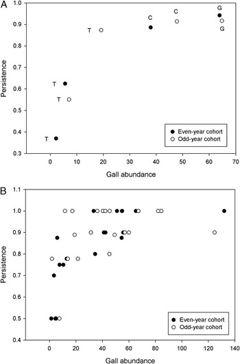
Considering low and high persistence cohorts at Tel Aviv separately, and pooling the high persistence cohorts at Tel Aviv with the cohorts from Carmel and Guvrin, the positive relationship between abundance and persistence was evident, and this relationship was nonlinear (Fig. 2A). The relationship was, however, approximately linear and positive when mean annual abundance was >10 galls per tree (R = 0.918, n = 5, P = 0.028; Pearson correlation). The one cohort from Tel Aviv with gall abundance above a threshold of about 10 galls per tree had a persistence consistent with the data from Carmel and Guvrin (Fig. 2A). The persistence of galls on the other trees at Tel Aviv, with abundance <10, declined sharply as abundance declined (Fig. 2A).
Relationships between persistence (proportion of years galls are present) and abundance (number of galls averaged over the time series) of Baizongia pistaciae galls, from even-year and odd-year cohorts, on Pistacia trees in Israel: A. Mean values for subpopulations at Carmel (C) and Guvrin (G), and for low-persistence (<0.5) and high-persistence (≥0.5) subpopulations at Tel Aviv (T); B. Estimates for 20 individual subpopulations and two cohorts from three populations, with persistence ≥0.5.

Population parameters for subpopulations with high persistence
To eliminate any numerical anomaly resulting from many 0-values, population parameters were re-estimated for the 20 subpopulations with high persistence: seven at Carmel; six at Guvrin; and seven at Tel Aviv. Persistence was 0.63 for one cohort at Tel Aviv, but otherwise 0.87–0.94 (Table 1). Gall abundance differed by up to 10 times among populations and also differed between cohorts (Table 1). The differences were detected in a mixed model analysis of variance: for populations (F = 7.9, df = 2, 17, P = 0.004) and cohorts (F = 8.5, df = 1, 19, P = 0.009). For these subpopulations, PV for one cohort at Carmel was 0.60, but otherwise was 0.67–0.72 (Table 1). No difference in PV was detected in a two-way analysis of variance with a nonsignificant interaction, neither among populations (F = 0.87, df = 2, 34, P = 0.43) nor between cohorts (F = 3.22, df = 1, 34, P = 0.08). For the region, the mean PV for B. pistaciae galls on individual trees with persistence ≥0.5 was 0.676 ± 0.015 (SE, n = 40).
For the 20 frequently colonised trees, the relationship between persistence and abundance was positive, with the lowest persistence occurring when a tree had fewer than 10 galls (Fig. 2B). Persistence increased with abundance (linear regression coefficient = 0.003, F = 21.7, df = 1, 38, P < 0.001). No relationship was detected between abundance and PV (linear regression coefficient = −0.001, F = 3.7, df = 1, 38, P = 0.061) or between PV and persistence (linear regression coefficient = −0.509, F = 3.4, df = 1, 38, P = 0.073), although in the latter case the regression coefficient was relatively large with P < 0.1, and negative as expected if persistence increases with PV.
Population stability and sampling interval
PV showed no consistent pattern with the length of the sampling interval for any of the locations (Table 3). For the “more-time–more-variation” hypothesis to be supported, regression coefficients would need to be consistently and significantly positive, which they were not. PV was regressed against the number of sexual generations for each cohort and subpopulation, as the length of the time series increased. The first two estimates of PV from the first three cycles in each time series were excluded because variation in PV was high as expected when only two to three sexual generations contributed to the estimate (Lamb and MacKay Reference Lamb and MacKay2010).
Frequency of positive (+) and negative (−) linear regression coefficients relating population variation (estimated by PV) in a time series to the length of the time series for individual subpopulations and cohorts.

A more-time–more-variation effect predicts a positive coefficient.
*Probability that the coefficient differs from 0.
Population stability and spatial scale
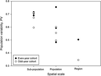
PV for B. pistaciae declined as the spatial scale increased, based on the 20 trees where galls were usually present (Fig. 3). For clarity, the plotted points at the subpopulation scale are the means from Table 1, rather than the 40 values for individual trees. At the population scale, the highest value is for Tel Aviv and the two lowest values are for Carmel and Guvrin (Fig. 3). Mean values for PV at the three spatial scales were as follows: subpopulation – 0.704 ± 0.013 (±1 SD, n = 20) and 0.659 ± 0.058 (±1 SD, n = 20); population – 0.610 ± 0.137 (±1 SD, n = 3) and 0.551 ± 0.052 (±1 SD, n = 3); region – 0.503 (n = 1) and 0.345 (n = 1), for even-year and odd-year cohorts, respectively. A one-way analysis of variance detected a reduction in PV from subpopulation (n = 40) to population (n = 6) scale (F = 5.51, df = 1, 44, P = 0.024). PV declined by about 15% from subpopulation to population and by 17% or more from population to regional scale.
Population variability (PV, defined in “Materials and methods”) of Baizongia pistaciae galls, from even-year and odd-year cohorts, on Pistacia trees at three spatial scales in Israel. For clarity, mean values for subpopulations (trees) at each location and for each cohort are plotted instead of the 40 individual estimates.

The decline in PV from subpopulation to population was associated with low correlations among the annual gall abundance for many of the subpopulations. At each of the three locations (6 or 7 subpopulations), one-third of the 57 possible Pearson correlation coefficients (all positive) comparing year-to-year gall abundance between pairs of subpopulations were significant (n = 17–20 years, P < 0.05). The decline in PV from population scale to regional scale also was associated with low correlations among the annual mean gall abundance for the three populations (Pearson correlation coefficients = 0.041, −0.089, −0.319; n = 16 years, P > 0.229). Synchronisation in abundance from year to year was weak between individual subpopulations within a population and absent between populations.
The persistence of B. pistaciae was relatively low at the subpopulation scale, particularly at Tel Aviv where many of the 24 trees were without galls in particular years (Table 1). At the population scale, however, galls were present every year in all three populations, although at Tel Aviv in 1988 only one gall was present on one of the 24 trees. With a persistence of one at the population scale, persistence was also one at the regional scale.
Habitat specificity of population parameters
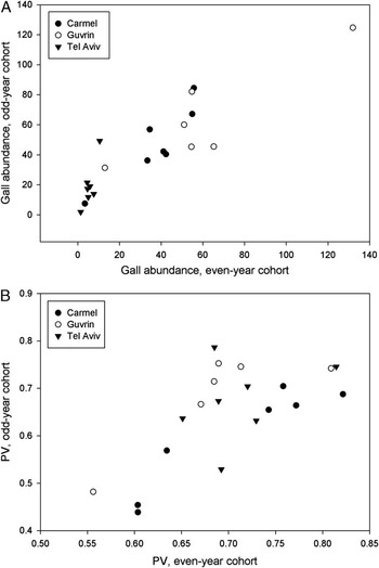
The even-year and odd-year cohorts had consistently low, intermediate, or high gall abundance on individual trees over the 8–10 cycles (Fig. 4A). PV was also characteristic of the subpopulation on an individual tree, with both cohorts having relatively low PV on some trees, and relatively high PV on other trees (Fig. 4B). For 20 subpopulations and two cohorts, PV ranged from 0.44 to 0.82. Considering individual subpopulations, gall abundance was positively correlated between cohorts in each population, PV was positively correlated between cohorts at Carmel and Guvrin, and even persistence with a narrow range of values was positively and highly correlated between cohorts at Carmel (Table 4). The consistency between cohorts was evident from the following examples: at Carmel, Tree 5 had three and eight galls, on average, whereas Tree 9 had 56 and 85 galls for the two cohorts; at Guvrin, Tree 16 had 13 and 31 galls, on average, whereas Tree 14 had 132 and 125 for the two cohorts; at Tel Aviv, Tree 18 had one and two galls, on average, whereas Tree 14 had 11 and 49 for the two cohorts. The trees with lowest and highest gall abundance in each population usually differed by an order of magnitude, for both cohorts. Similar patterns of difference in PV were observed. Nevertheless, no relationship was detected between abundance and PV; individual subpopulations with similar gall abundance did not necessarily have similar PV (Table 2).
Relationships between even-year and odd-year cohorts of Baizongia pistaciae for gall abundance (average number of galls over time) (A); and population variability (PV, defined in “Materials and methods”) (B), for 20 subpopulations with high persistence (≥0.5) on individual Pistacia trees, from three populations in Israel.

Pearson correlation coefficients, followed by the probability that the coefficient = 0 in parentheses, between the even-year and odd-year cohorts of Baizongia pistaciae galls on Pistacia trees at three locations in Israel, for three population parameters (abundance, population variability, and persistence) estimated for individual subpopulations (trees).

PV quantifies population variability.
Discussion
Three populations of B. pistaciae persisted throughout the 17–20-year study, and so were in that sense stable. PV, however, was relatively high: PV was 0.581 ± 0.040 (SE) with a range of 0.483–0.755 (n = 6). This level of PV is similar to that of two other native aphids, Uroleucon rudbeckiae (Fitch) with PV = 0.648 ± 0.036 (SE) (Lamb and MacKay Reference Lamb and MacKay2010) and Macrosiphum euphorbiae (Thomas) with PV = 0.585 (Lamb et al. Reference Lamb, MacKay and Alyokhin2011). Thus, the more permanent tree–grass habitat and galling habit of B. pistaciae did not stabilise its populations as expected, when compared with free-living native aphid species on herbaceous foliage. Although the primary host of B. pistaciae is a long-lived tree, the secondary host is a grass (Wool Reference Wool2004). Temporal variation in the proximity of alternate hosts (Martinez et al. Reference Martinez, Mokady and Wool2005) or other aspects of the complex interaction between alternate hosts may destabilise populations of B. pistaciae. If host-alternation is indeed destabilising, the population dynamics of aphid species that use only trees as hosts would be expected to have lower PV than B. pistaciae.
Lamb et al. (Reference Lamb, MacKay and Alyokhin2011) note that two native species of aphids have lower PV than two introduced species. The PV of the native B. pistaciae also is lower than that of two introduced aphid species, Myzus persicae (Sulzer) (PV = 0.771) and Aphis nasturtii (Kaltenbach) (PV = 0.831) (Lamb et al. Reference Lamb, MacKay and Alyokhin2011), consistent with other native species. More examples of native and introduced aphid species are required to confirm this generality.
Parameters that define the population dynamics of species are thought to be interrelated, reflecting the density-dependent processes that underlie them (Taylor and Woiwod Reference Taylor and Woiwod1980). For example, low population persistence is hypothesised to be a consequence of high population variability (Inchausti and Halley Reference Inchausti and Halley2003). For B. pistaciae, however, no consistent relationship was detected between persistence and population variability. The trend of persistence with PV for subpopulations with persistence ≥0.5 was negative, as expected, but not significant. For trees with persistence <0.5, persistence increased with PV, contrary to expectations, probably because of the numerical relationships among parameters when a time series has many 0-values for abundance. At the population scale, low and high persistence populations had essentially the same PV. However, persistence of B. pistaciae was associated with abundance: persistence was low when average abundance was low. Reduced persistence is also more closely associated with low abundance than high population variability for four other species of aphid (Lamb and MacKay Reference Lamb and MacKay2010; Lamb et al. Reference Lamb, MacKay and Alyokhin2011) and for some spiders (Schoener and Spiller Reference Schoener and Spiller1987). PV, however, was unrelated to abundance at the subpopulation or population scale. The independence of persistence and PV, and the difference in the relationships between persistence and abundance in comparison with PV and abundance support the idea that persistence and population variability are distinct components of stability, determined by different aspects of the population dynamics of a species.
Population variability has been hypothesised to increase with time, the more-time–more-variation effect (Lawton Reference Lawton1988; Pimm and Redfearn Reference Pimm and Redfearn1988; Inchausti and Halley Reference Inchausti and Halley2002). No consistent increase in PV was detected for B. pistaciae, however. A similar lack of increase in variation with time was observed in populations of four other aphid species (Lamb and MacKay Reference Lamb and MacKay2010; Lamb et al. Reference Lamb, MacKay and Alyokhin2011). The 17–20 years, 8–10 iterations of the 2-year life cycle, represents a long study in practical terms, but may be too short to detect a more-time–more-variation effect.
Population variability of the two cohorts of B. pistaciae declined as the scale of the study increased. A decline is expected if differences in year-to-year fluctuations for different subpopulations or populations average out because they are asynchronous (Connell and Sousa Reference Connell and Sousa1983). Indeed, few correlations between annual abundance were detected between subpopulations even when trees were relatively near to each other, and none were detected between populations of B. pistaciae. The fluctuations of these populations are independent of and therefore not synchronised by weather (Wool Reference Wool2002). In contrast, subpopulations and populations of U. rudbeckiae are highly synchronised and show no decline in population variability as spatial scale increases (Lamb and MacKay Reference Lamb and MacKay2010). Population variability declines with scale but probably only when populations do not fluctuate in synchrony.
The contrast in the effect of spatial scale on population variability between B. pistaciae and U. rudbeckiae suggests that interspecific comparisons need to be made between equivalent scales. A subpopulation of B. pistaciae includes the galls on an individual tree, whereas a subpopulation of U. rudbeckiae includes the colonies on a group of stems in a patch of plants. The mean number of galls per tree varied from 2 to 65, on average, numerically similar to the number of U. rudbeckiae colonies in a patch of host plants (Lamb and MacKay Reference Lamb and MacKay2010). A population of B. pistaciae consists of the galls on a group of adjacent trees along a few kilometres of road, whereas a population of U. rudbeckiae consists of the colonies on a group of plant patches along 1–3 km of trail (Lamb and MacKay Reference Lamb and MacKay2010). For these two aphid species, the spatial scales relative to the sampling scale and the abundance of aphids in the sampling units are equivalent. However, where spatial scales are not ecologically equivalent, interspecific comparisons are questionable: for example, for comparisons between species with different dispersal capacities or from habitats with different spatial characteristics.
PV is often considered to be a species characteristic (Taylor and Woiwod Reference Taylor and Woiwod1980). For the few aphid species studied, species-specificity is supported either because PV is uniform among spatial scales and populations for U. rudbeckiae (Lamb and MacKay Reference Lamb and MacKay2010), or because PV is consistently different among species from decade to decade for three potato-colonising aphid species living in the same habitat (Lamb et al. Reference Lamb, MacKay and Alyokhin2011). At the subpopulation spatial scale, B. pistaciae also shows similar PV, on average, among populations and between cohorts. However, PV at the population scale, ranging from 0.48 to 0.76, is less uniform than might be expected if it is primarily a species trait. Perhaps more importantly, subpopulations on individual trees show characteristic abundances and PV, based on the correlation between cohorts for each of these two parameters. At the subpopulation scale, the population variability of B. pistaciae depends at least in part on characteristics of the habitat it finds itself in, the specific tree and associated secondary host grass. Furthermore, the aphid itself is an important factor in shaping the quality of its habitat through its effect on the architecture of its primary host. Kurzfeld-Zexer et al. (Reference Kurzfeld-Zexer, Wool and Inbar2010) find that infestation of Pistacia trees by B. pistaciae early in a tree's life changes its growth form from tree shape to multi-stemmed shrub shape, and the shrubby form is more susceptible to subsequent infestation by the aphid than the tree form. Thus, at the subpopulation scale, population variability results from the interaction of the aphid with its habitat. Nevertheless, differences in PV among subpopulations average out so that the mean PV for different populations is similar. The interaction between aphid and its tree–grass habitat must be similar, on average, for the three locations. This characteristic level of population variability is maintained in different populations even though genetic differentiation occurs among populations, which results from limited dispersal by the aphid (Martinez et al. Reference Martinez, Mokady and Wool2005).
The unique abundance and stability properties of B. pistacia on individual trees might be due to the resistance level of the tree to the aphid, some site-specific or tree-specific habitat characteristic (e.g., proximity to patches of the secondary grass host), or genetic differentiation of the aphids that use that tree (Martinez et al. Reference Martinez, Mokady and Wool2005). The importance of individual trees or tree–grass units of habitat in determining the dynamics of the subpopulation is shown by the similar dynamics of the two genetically independent cohorts. Interestingly, population variability is not related to abundance, confirming that for B. pistaciae, as for the aphids studied previously (Lamb and MacKay Reference Lamb and MacKay2010; Lamb et al. Reference Lamb, MacKay and Alyokhin2011), both parameters must be quantified to define the population dynamics of a species.
Baizongia pistaciae forms a large gall on its primary host, a Pistacia tree, and alternates with the roots of its secondary host, a grass, in a 2-year life history (Wool Reference Wool2004). It interacts with individual long-lived host trees in a way that results in genetic differentiation at the subpopulation scale (Martinez et al. Reference Martinez, Mokady and Wool2005). The aphid causes phenotypic changes in the host that alter the subsequent suitability of the host to the aphid (Kurzfeld-Zexer et al. Reference Kurzfeld-Zexer, Wool and Inbar2010). In spite of the marked difference between this life history and that of native aphid species that feed as free-living herbivores on ephemeral herbaceous hosts (Lamb and MacKay Reference Lamb and MacKay2010; Lamb et al. Reference Lamb, MacKay and Alyokhin2011), stability measured as population variability and persistence is remarkably similar for B. pistaciae and these other native aphids. Persistence of B. pistaciae decreases as average abundance decreases but is not related to population variability, and population variability does not increase with the length of the study. The same relationships have been observed for other aphid species (Lamb and MacKay Reference Lamb and MacKay2010; Lamb et al. Reference Lamb, MacKay and Alyokhin2011). Unlike U. rudbeckiae (Lamb and MacKay Reference Lamb and MacKay2010), the population variability of B. pistaciae declines with population scale, because abundance of the former species is synchronised among subpopulations and populations, whereas the population fluctuations of the latter species are not. The PV of B. pistaciae, like that of other aphid species, is relatively high, above 0.5 on a scale of 0–1, and clearly reflects an important trait of the population dynamics of the species, independent of average abundance.