
I. INTRODUCTION
Instrumented (depth-sensing) indentation is extensively used nowadays for the characterization of local mechanical properties of various materials including metals, ceramics, polymers, or composites. Reference Doerner and Nix1 This method can be performed on very small and/or thin specimens by applying very small loads resulting in depths at the nanometer scale. Reference Menčík, Munz, Quandt, Weppelmann and Swain2 The principal goal of this method is to extract hardness and Young's modulus from the indenter load versus depth of penetration profile. The most commonly used method is the Oliver and Pharr method Reference Oliver and Pharr3,Reference Oliver and Pharr4 which forms the basis for the instrumented indentation testing standard [ISO 14577 (Ref. 5)].
This procedure is founded upon elastic solution of contact problem (Sneddon's solution Reference Sneddon6 ). An underlying assumption of this method is that the indented solid body is homogeneous and isotropic. When indenting in proximity of an interface between two phases with different properties, this assumption is no longer valid. However, the instrumented indentation of structurally heterogeneous materials using Oliver–Pharr method is frequently used to characterize the properties of individual phases as this method is simple and available in practically all commercial devices.
One way of characterizing the microstructurally heterogeneous materials is the positioning of isolated indentations (e.g., with the aid of light microscopy) inside the individual phases, sufficiently far from the interface, which permits to obtain the properties of single phases. Another way is the grid indentation which is based on performing a large number of equidistantly spaced indentations and their statistical evaluation. Reference Constantinides, Ravi Chandran, Ulm and Van Vliet7,Reference Randall, Vandamme and Ulm8 Both methods need the knowledge of so called indentation length scale since it has been shown many times that the particle size, shape, and properties do influence the indentation response. Generally, the experimental conditions choice is made such that the indentation depth is lower than a critical indentation depth below which microstructural length scales do not interfere significantly with the indentation response, and hence the indentation data acquired to such a depth provide access to the intrinsic properties of the material. Nevertheless, the indentation in proximity of the interface cannot always be completely avoided—in the grid indentation, the position of some indents can coincide with the phase boundary, or the invisible phase boundary can be close below the indenter contact area, which can by the way occur for both grid and isolated indentations.
An often-used rule of thumb limits the maximum indentation depth to one 10th of the film thickness. In two-phase materials, a similar depth limit can be defined by dividing the contact radius with the particle radius. Reference Durst, Göken and Vehoff9 However, a critical indentation depth with respect to the size of the heterogeneity depends also on the phase geometry and modulus (and other mechanical properties) mismatch.
For the isolated indentation, the load versus depth of penetration curves which show a transition from characteristic soft to hard loading behavior (and vice versa), should be excluded from the analysis. Reference Constantinides, Ravi Chandran, Ulm and Van Vliet7,Reference Durst, Göken and Vehoff9 For the grid indentation technique, it is frequently much more difficult to exclude all the influenced measurements. When applying the statistical evaluation of results, e.g., a bimodal Gaussian fit, the presence of boundary-affected results leads to the bias of the distribution, i.e., to an overestimation of the softer phase hardness and/or modulus together with an underestimation of harder phase values. Reference Haušild, Nohava and Pilvin10 Some improvements were achieved taking an interface as an “extra” phase with a flat Gaussian distribution. Reference Nohava, Haušild, Houdková and Enžl11 However, this is not correct as the change of materials behavior definitely does not follow the Gaussian distribution. Moreover, it leads to three more parameters, which exceedingly complicates the identification procedure as it necessitates huge amount of data.
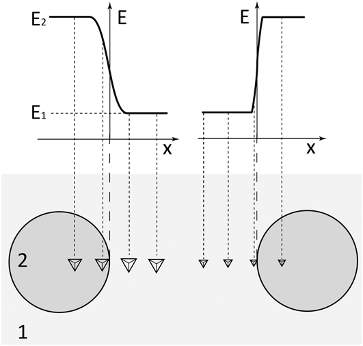
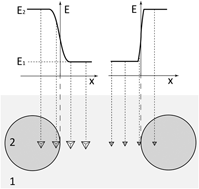
The aim of this paper is to present a case study on two-phase materials with distinctly different hardness and Young's modulus (metal–metal, ceramic–ceramic, and metal–ceramic composites). The influence of depth of penetration and microstructural length scale on the measured indentation modulus distribution was incorporated via presence of transitional zone with a progressive change of materials behavior (Fig. 1).
Transition from hard to soft or soft to hard measured (apparent) properties when indenting across the interface between two phases (1, 2) with unlike Young's moduli (E 1, E 2) using different size of indents (depth of penetrations).

The probability of indentation in the affected area as a function of depth of penetration and size of particles was simulated by finite element computations and fitted by a statistical distribution function. Subsequently, this approach was experimentally verified by indentation in proximity of the boundary between the phases with distinctly different mechanical properties. Finally, the intrinsic properties of the material were successfully extracted from the experimental grid indentation data.
II. THEORETICAL BACKGROUND OF THE MODEL
When indenting near the interface between two phases with different properties, the measured values (hardness or Young's modulus) can be affected by two principal factors. The first factor can be associated with the material property and the second one with the experimental method. To understand the effect of an interface on the distribution of measured indentation data, it is convenient to briefly summarize the idealized cases.
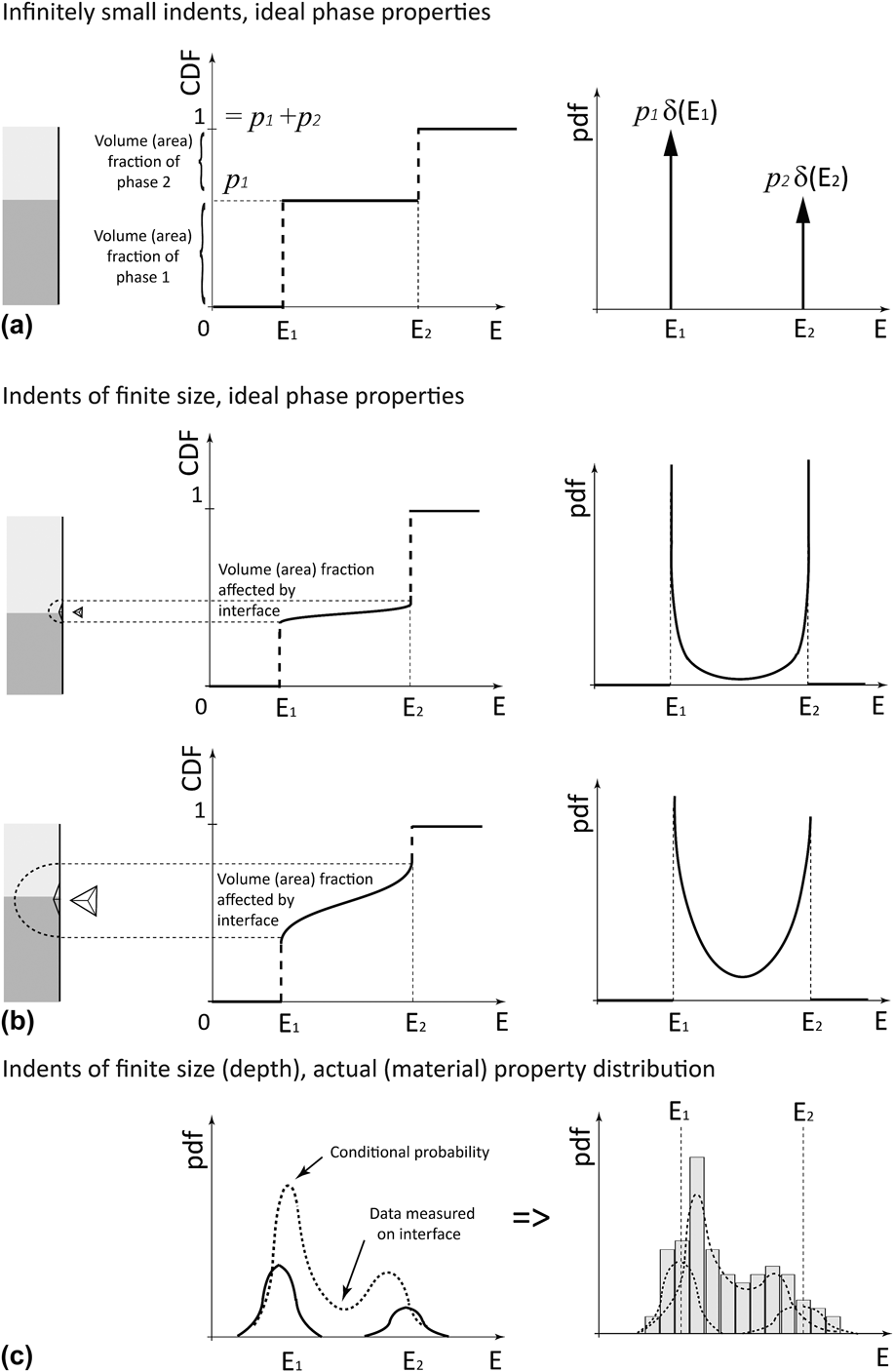
The first case corresponds to measuring with “ideal” indenter (with point contact, affecting infinitesimally small volume under the indenter, and introducing no scatter to the evaluation method) on a composite of two “ideal” materials (with no scatter in material properties). The obtained cumulative distribution function (CDF) is then characterized by two jump discontinuities at properties 1 and 2 (i.e., Heaviside step functions), and probability density function (pdf) involves two Dirac delta functions as can be illustrated e.g., for Young's modulus in Fig. 2(a) and Eq. (1):
 $${\rm{pdf}}\left( E \right) = {p_1}\delta \left( {{E_1}} \right) + {p_2}\delta \left( {{E_2}} \right)\quad ,$$
where p 1 and p 2 are the volume/area fraction of the phase 1 and 2 respectively (p 1 + p 2 = 1), E 1 and E 2 are the Young's moduli of the phase 1 and 2, respectively.
Idealized distributions of measured (apparent) properties when indenting in material containing an interface between two phases with unlike Young's moduli (a, b) and actual distribution affected by measuring near the interface (c).
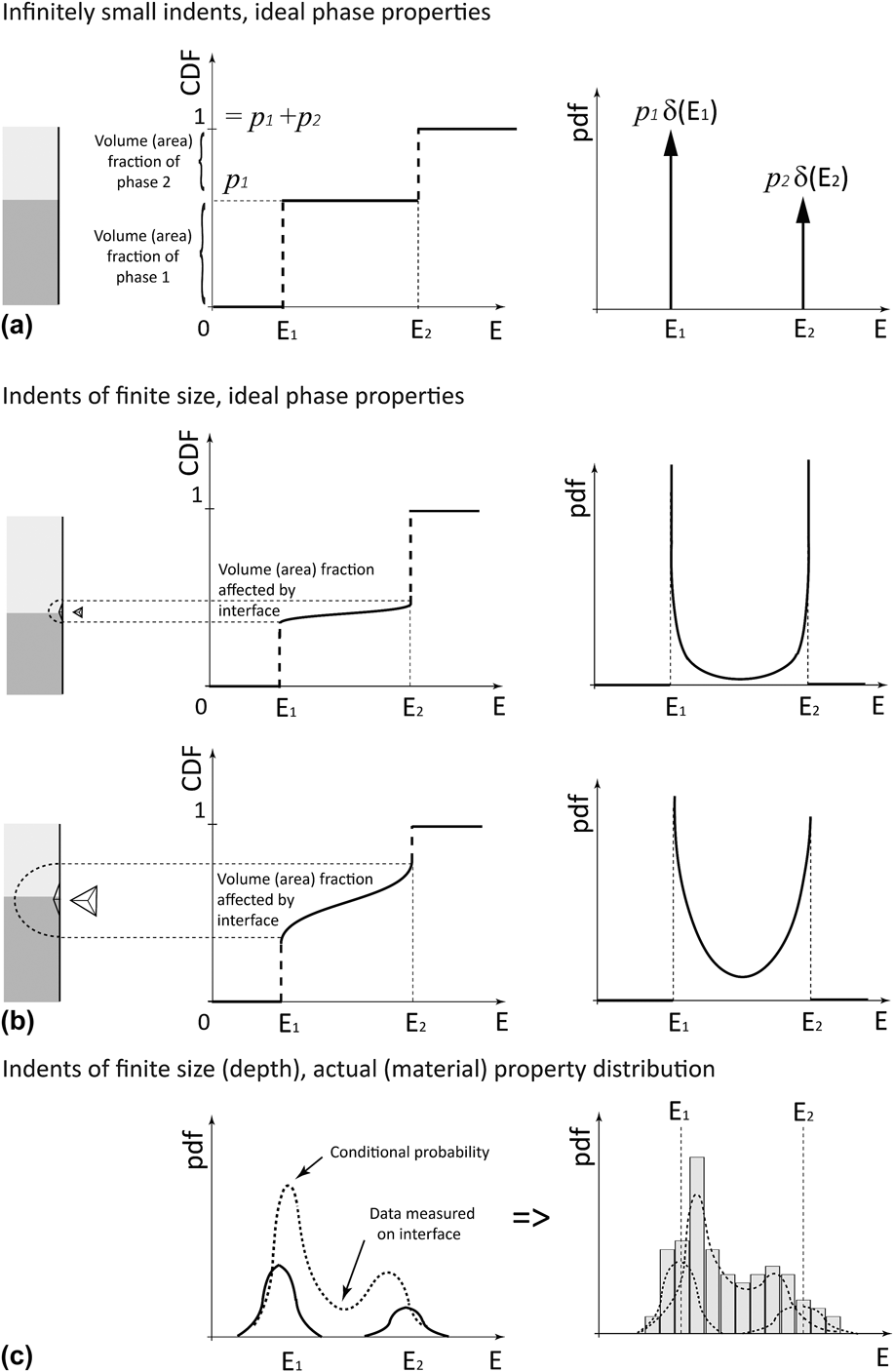
In the next case, all conditions are the same (no scatter in material properties and/or in experimental method), except the fact that the stress field induced by the indentation affects the volume under and next to the contact area. Measurement across the boundary between two phases therefore depends on the size (depth) of the indent as it is illustrated in Fig. 1. The cumulative distribution function must then incorporate this S-shape transition from one material property to the other in the volume/area fraction affected by the presence of the interface. In the limiting case when the volume/area fraction affected by the presence of the interface approaches to zero, the distribution shall tend to precedent case. These conditions are effectively fulfilled by using the beta distribution with the probability density function:
 $${\rm{pdf}}\left( x \right) = {{{x^{a - 1}}{{\left( {1 - x} \right)}^{b - 1}}} \over {B\left( {a,b} \right)}}\quad ,$$
which is defined for x from the interval 〈0,1〉, the shape parameters a and b are from the interval 〈0,1〉 to ensure the U-shape of the probability density function [Fig. 2(b)]. When the parameters a → 1 and b → 1, this probability density function tends to form like that of uniform distribution. Decreasing parameters a and b lead to narrower transition from one material property to the other [i.e., decrease of the volume/area fraction affected by the presence of the interface as shown in Fig. 2(b)]. When the parameters a → 0 and b → 0, the probability density function tends to form two Dirac delta functions. Normalization constant B(a,b) is given by the beta function (Euler integral of the first kind):
 $$B\left( {a,b} \right) = \int\limits_0^1 {{x^{a - 1}}{{\left( {1 - x} \right)}^{b - 1}}{\rm{d}}x\quad } .$$
It will be shown later that the change of materials behavior measured by indentation across the interface can effectively be approximated by inverse beta distribution, so that the (normalized) measured values can be statistically described by:
 $${\rm{pdf}}\left( E \right) = {{{{\left( {{{E\, -\, {E_1}} \over {{E_2} \,-\, {E_1}}}} \right)}^{a - 1}}{{\left( {1 - {{E \,-\, {E_1}} \over {{E_2} \,-\, {E_1}}}} \right)}^{b - 1}}} \over {\left( {{E_2} - {E_1}} \right)B\left( {a,b} \right)}}$$
for
 ${E_1} \lt\, {E_2}$
,
 $E \in \left( {{E_1},\;{E_2}} \right)$
, elsewhere
 ${\rm{pdf}}\left( E \right) = 0$
.
In the third case, measuring indenter with point contact and affecting infinitesimally small volume under the indenter is assumed; however, scatter in material properties of both phases can be introduced for example, by different crystallographic orientation, Reference Vlassak and Nix12–Reference Materna, Haušild and Nohava15 state of the surface or for example, by the experimental device. Reference Menčík and Swain16,Reference Menčík and Swain17 The obtained (bimodal) distribution can then be mixed from two Gaussian distribution.
 $${\rm{pdf}}\left( E \right) =\; {{{p_1}} \over {\sqrt {2\pi } {\sigma _1}}}\exp \left[ { - {{{{\left( {E - {{\overline E }_1}} \right)}^2}} \over {2\sigma _1^2}}} \right] + {{{p_2}} \over {\sqrt {2\pi } {\sigma _2}}}\exp \left[ { - {{{{\left( {E - {{\overline E }_2}} \right)}^2}} \over {2\sigma _2^2}}} \right]\quad ,$$
where parameters
 ${\overline E _1}$
,
 ${\overline E _2}$
represent mean values of Young's moduli and the σ1, σ2 scatter of Young's moduli in the phases 1 and 2.
Combining the second and third case, i.e., assuming the “real” indenter (of finite size) and scattered material properties, the resulting data distribution is given by conditional probability of measuring in phase 1, 2, or near the interface between phase 1 (with actual material property 1) and phase 2 (with actual material property 2):
 $${\rm{pdf}}\left( E \right) = {{{p_1}} \over {\sqrt {2\pi } {\sigma _1}}}\exp \left[ { - {{{{\left( {E - {{\overline E }_1}} \right)}^2}} \over {2\sigma _1^2}}} \right] + {{{p_2}} \over {\sqrt {2{\rm{\pi }}} {\sigma _2}}}\exp \left[ { - {{{{\left( {E - {{\overline E }_2}} \right)}^2}} \over {2\sigma _2^2}}} \right] +\, {p_3}\int\limits_{ - \infty }^{ + \infty } {{\kern 1pt} {\kern 1pt} \int\limits_{ - \infty }^{ + \infty } {{{{{\left( {{{E \,-\, {E_1}} \over {{E_2} \,-\, {E_1}}}} \right)}^{a - 1}}{{\left( {1 - {{E \,-\, {E_1}} \over {{E_2} \,-\, {E_1}}}} \right)}^{b - 1}}} \over {\left( {{E_2} - {E_1}} \right)B\left( {a,b} \right)}}} } \;{1 \over {\sqrt {2\pi } {\sigma _1}}}\exp \left[ { - {{{{\left( {{E_1} - {{\overline E }_1}} \right)}^2}} \over {2\sigma _1^2}}} \right]{1 \over {\sqrt {2\pi } {\sigma _2}}}\exp \left[ { - {{{{\left( {{E_2} - {{\overline E }_2}} \right)}^2}} \over {2\sigma _2^2}}} \right]{\rm{d}}{E_1}{\rm{d}}{E_2}\quad ,$$
where p 3 is the volume/area fraction affected by the presence of the interface, other parameters were explained in previous equations.
This case is closest to the reality and will be considered in the following paragraphs.
III. VALIDATION METHODOLOGY
A. Experimental details
The samples chosen for this case study were two-phase composites with different combinations of materials: metal–metal (tungsten-SS410 steel), ceramic–ceramic (yttria-stabilized zirconia, YSZ–Al2O3), and metal–ceramic (FeAl–Al2O3). In all these composites, both constituents have distinctly different Young's modulus (about two times) and distinctly different hardness. The selected materials do not present important pile-up phenomenon and can therefore be advantageously characterized using Oliver and Pharr method.
Cylindrical samples (of 25 mm diameter and 8 mm height) were prepared by spark plasma sintering on Thermal Technology SPS 10-4 machine (Thermal Technology LLC, Santa Rosa, California) from (commercially supplied) pure powders: W (OSRAM Sylvania, Towanda, Pennsylvania), SS410 steel (Flame Spray Technologies, Duiven, The Netherlands), Fe29Al (LERMPS, Belfort, France), Al2O3 (Korund Benátky, Benátky nad Jizerou, Czech Republic), YSZ (H.C. Starck, Munich, Germany). The sintering conditions (sintering temperature, piston pressure, and sintering time) were: tungsten-steel 1100 °C/80 MPa/2 min, FeAl–Al2O3 1100 °C/60 MPa/5 min, YSZ–Al2O3 1600 °C/60 MPa/5 min. These conditions were optimized to obtain minimum porosity and to prevent the formation of any interlayer at the interface between the parent phases as for example, the Fe7W6 intermetallic compounds in the case of W-steel composite.
The sample surfaces were subsequently ground and polished with final step in 0.05 µm noncrystallizing amorphous colloidal silica suspension to avoid the surface layer affected by mechanical grinding and polishing.
Nanoindentation measurements were performed on CSM NHT Nanoindentation Tester (Anton Paar TriTec SA, Pesseux, Switzerland) with Berkovich indenter. The results were evaluated according to Oliver and Pharr method. Reference Oliver and Pharr3,Reference Oliver and Pharr4 In this method, the unloading (i.e., elastic) part of load–displacement data is fitted by power law:
 $$P = {\rm{\alpha }}{\left( {h - {h_{\rm{f}}}} \right)^m}\quad ,$$
where P is the load, h is the depth, h f is the final depth after unloading, α and m are parameters fitted by least square method.
The slope of the tangent to the data at maximum load dP/dh is then determined and inserted into Eq. (8) to give the contact depth h c:
 $${h_{\rm{c}}} = {h_{\max }} - \varepsilon {{{P_{\max }}} \over {{\rm{d}}P/{\rm{d}}h}}\quad ,$$
where the geometric constant ε is given for the conical indenter by ε = 2(π − 2)/π ∼ 0.72 (for flat punch ε = 1, and for the paraboloid of revolution ε = 0.75). Reference Fischer-Cripps18
The contact area A is then found from the geometry of the indenter as a function of the contact depth h c using the formula:
 $$A = {C_0}h_{\rm{c}}^2 + {C_1}{h_{\rm{c}}} + {C_2}h_{\rm{c}}^{{1 \mathord{\left/ {\vphantom {1 2}} \right. \kern-\nulldelimiterspace} 2}} + {C_3}h_{\rm{c}}^{{1 \mathord{\left/ {\vphantom {1 4}} \right. \kern-\nulldelimiterspace} 4}} + \ldots + {C_8}h_{\rm{c}}^{{1 \mathord{\left/ {\vphantom {1 {128}}} \right. \kern-\nulldelimiterspace} {128}}}$$
proposed in Ref. Reference Oliver and Pharr3 and recommended by the standard. 5 The coefficients of the area function C 0…C 8 were determined by calibration on material with known Young's modulus (fused silica). The indentation hardness H IT, and the reduced modulus E * can be then calculated as:
 $${H_{{\rm{IT}}}} = {{{P_{\max }}} \over A}\quad ,$$
 $${E^ * } = {{\sqrt \pi } \over {2\beta \sqrt A }}{{{\rm{d}}P} \over {{\rm{d}}h}}\quad ,$$
where β is dimensionless correction factor applied since the elastic recovery of material upon removal of load leads to some significant deviations in the expected shape of the unloading portion of the load–displacement curve. Reference Hay, Bolshakov and Pharr19
The reduced modulus E * is related to Young's moduli of the specimen (E) and the indenter (E i ) by:
 $${1 \over {{E^*}}} = {{\left( {1 - {\nu ^2}} \right)} \over E} + {{\left( {1 - \nu _i^2} \right)} \over {{E_i}}}\quad ,$$
where ν and ν i are Poisson's ratios of the specimen and the indenter, respectively.
So-called continuous multicycle (CMC) indentations consisting of progressive loading with partial unloading were used to obtain indentation modulus for different loads (from different depths) at the same positions. The indentation parameters were chosen from preliminary experiments (single indentations at maximum load) to fulfill the conditions: (i) cover sufficiently the area containing both phases, (ii) do not influence other measurements (i.e., keep the distance between the indents at least at 3 times the size of final imprints).
First, the indentations were performed in known distances from the interface. For W-steel composite, the sample with a sharp interface oriented parallel to the surface normal (indenter axis) was prepared (both materials have practically the same Poisson's ratio and moderately different coefficients of thermal expansion, which resulted in good bonding along the interface). In the case of metal–ceramic and ceramic–ceramic composites, such sharp interface is hard (or impossible) to produce, so the indentations were performed near the particle boundaries (it should be noted that the interfaces under the surface were not necessarily oriented parallel to the indenter axis).
Next, several matrices of (10 × 10, 10 × 20, or 20 × 20) equidistantly spaced CMC indentations (of 4–6 load levels) were performed on rectangular areas of dimensions varying in dependence of the size of composite phases. After the indentations, the areas were examined with the aid of light microscope Neophot 32 (Carl Zeiss AG, Jena, Germany) and scanning electron microscope (SEM) JSM 5510LV (JEOL Ltd., Tokyo, Japan). The matrices of indentations are illustrated in Fig. 3, where the microstructures are also shown.
SEM micrographs (backscattered electrons signal) showing examples of grid indentations matrices (at the highest loads of continuous multicycle) in composites under the study. In the case of indentation near the tungsten-steel interface, the lines of indents were intentionally inclined to obtain well defined variation of distance from the interface.

The measured indentation moduli are presented in the form of plain strain indentation modulus to eliminate the effect of (a priori unknown) different Poisson's ratios of the analyzed phases:
 $$E_{{\rm{IT}}}^ * = {{{E_{{\rm{IT}}}}} \mathord{\left/ {\vphantom {{{E_{{\rm{IT}}}}} {\left( {1 - {\nu ^2}} \right)}}} \right. \kern-\nulldelimiterspace} {\left( {1 - {\nu ^2}} \right)}}\quad .$$
B. FEM analysis
Forward FEM analyses were carried out in MSC.Marc 2015 FEM code 20 to evaluate the effect of an interface on the apparent (measured) material property. For the evaluation of simulated load–displacement curves we adopted the method described above. The model was composed of 74,160 eight-node (3D) linear brick elements (78,620 nodes) and contained two distinct parts with different material properties (ideal material interface was assumed). Using symmetry, only one half of the specimen was modeled. Model size was chosen large enough to minimize effects of boundary conditions on the indented zone (more than 100 times the maximum indentation depth h max in each direction). Displacement of nodes on the bottom of the specimen was restricted in the direction of loading. Mesh size in the contact domain was optimized to be sufficiently fine (∼h max/10) with reasonable computation time. Positions of interface versus indenter as well as the mesh geometry in the contact domain are illustrated in Fig. 4. For the modeling of Berkovich indenter we used an equivalent conical indenter with a half-apical angle of 70.3°. Reference Fischer-Cripps18 The indenter was modeled by a rigid contact surface (with no friction). Elasticity in the indenter was neglected since it is important only for very hard materials (comparable to diamond).
Schematic sketch of the FEM mesh in the contact domain showing the position of the indenter with respect to the interface between two phases.

Simulations were carried out using elastic and elastic–plastic material formulation. For the elastic–plastic task, the stress σ for σ > σ y was defined as:
 $$\sigma = {\sigma _y}{\left( {1 + {E \over {{\sigma _y}}}{\varepsilon _{\rm{p}}}} \right)^n}\quad ,$$
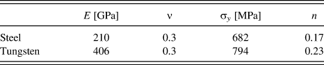
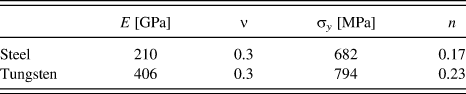
where εp is plastic strain, σ y is (0.2% offset) yield strength, and n is a strain-hardening exponent. Material parameters used in the elastic and elastic–plastic simulations were taken from Ref. Reference Matějíček, Nevrlá, Čech, Vilémová, Klevarová and Haušild21 (see Table I).
Material properties used in the elastic and elastic–plastic simulations. Reference Matějíček, Nevrlá, Čech, Vilémová, Klevarová and Haušild21
The first half of unloading part of the load–displacement curve was fitted by the power–law model in the form of Eq. (7). The derivative of P–h curve at the point of maximum load dP/dh served as a direct input for computation of indentation moduli using Eq. (11), where correction factor β was set to 1.067 (the same value as obtained by Hay et al. Reference Hay, Bolshakov and Pharr19 ) according to simulation with isotropic material so that the contact area A could be directly derived from the conical geometry of the indenter:
 $$A = \pi {\left( {{h_c}\,\tan \,70.3^\circ } \right)^2}\quad.$$
The contact depth h c was evaluated using Eq. (8), supposing ε = 0.72.
IV. RESULTS AND DISCUSSION
A. Indentation across the interface
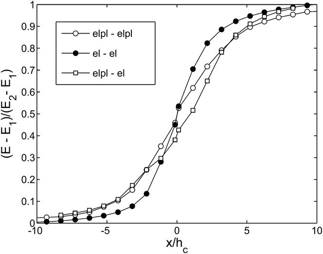
Results of indentations with different positions of interface versus indenter simulated by FEM are shown in Fig. 5. It can be seen that in the case of simulations with elastic formulation, the self-similar nature of the task enables the normalization of distance from the interface by contact depth x/h c. The change of indentation modulus measured by indentation across the interface can then be well approximated by symmetrical inverse beta distribution. The elastic–plastic simulations of indentations (using material parameters listed in previous section) lead to only slight deviation from the (symmetrical) inverse beta distribution fit. To note also the fact that for x/h c > 10 the effect of interface has completely vanished. The “interface affected region” is only slightly larger in the case of elastic–plastic materials than in elastic ones. The most “severe” situation is the combination of soft plastic and hard elastic materials on each side of the interface (this can occur e.g., in the case of ceramic particles reinforced metal matrix composites such as Al–Al2O3). However, even in the elastic/elastic–plastic case the approximation by (nonsymmetrical) inverse beta distribution seems to be reasonable (at least for the material parameters from Table I). Unfortunately, it is hard to relate directly the parameters of nonsymmetrical inverse beta distribution to hardness or indentation modulus of parent phases as they depend on overall material behavior in rather complex way (E, σ y , n, E/σ y …).
The change of normalized indentation modulus computed by FEM across the interface between elastic/elastic, elastic–plastic/elastic–plastic, and elastic/elastic–plastic materials as a function of normalized distance from the interface.

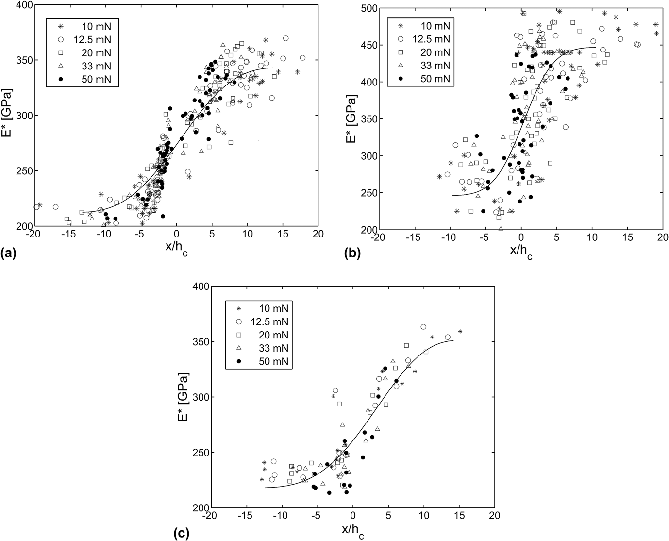
As a first approximation, it was therefore assumed that the results of experimental measurements across the interface can be assessed by symmetrical inverse beta distribution (with parameters a = b). First, the indentations on the W-steel sample with sharp interface oriented perpendicular to the surface of the sample and parallel to the indenter axis (Fig. 3) were performed. The indentation moduli measured by applying different loads in varying distances from the interface are shown in Fig. 6(a). It can be seen that for the same normalized distances x/h c the measured values are not dependent on applied load, which is in agreement with the FEM simulations.
The change of plain strain indentation modulus measured across the interface between (a) metal–metal (tungsten-steel), (b) metal-ceramic (FeAl–Al2O3), and (c) ceramic–ceramic (YSZ–Al2O3) composites.

In the next step, the same experiments were carried out on particulate composites. In this case, the spatial orientation of the interface is a priori unknown (not necessarily perpendicular to the surface and parallel to the indenter axis) and some part of particles can be hidden under the surface. Even if the previously developed model was built on the consideration of layered structure indented perpendicularly, the measured dependencies across the W-steel interface were very similar for the layered and particulate composites, and the sizes of zones influenced by presence of adjacent phase differed only very little.
The size of the transitional zone defined by distance at which 5% increase/decrease from the single phase indentation modulus mean values occurs was less than 20h c. In the case of metal–ceramic (FeAl–Al2O3) and ceramic–ceramic (YSZ–Al2O3) composites, the evolution of indentation modulus across the interface was only little steeper (the size of the transitional zone was less than 15h c) and the shape of the transition was quite similar [Figs. 6(b) and 6(c)]. It is to note that so computed or experimentally obtained sizes of the transitional zones can serve for rough estimation of the area/volume fraction affected by the presence of interface for known microstructure (with known boundary length) and, therefore, for optimizing the choice of the penetration depth (maximum load) in the grid indentation. Nevertheless, as it has already been stated in previous sections, the indentation in proximity of the interface cannot be completely avoided as the surface roughness and particle size and shape impose limitations on the suitable depth of indentation.
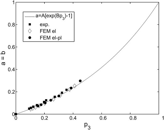
The evolutions of indentation modulus across the interface obtained by FEM and/or experimentally were subsequently used to reproduce the interaction of real two-phase microstructure with the indentation at different load. By varying the range of x/h c on which the inverse beta distribution fit was performed (i.e., the ratio between particle size and depth of indentation), the different area/volume fraction affected by the presence of interface can be simulated. The dependence of fitted beta distribution parameter a (=b) on the size (resp. fraction) of the transition zone is shown in Fig. 7. This dependence can be effectively fitted by exponential relation:
 $$a = A\left[ {\exp \left( {B{p_3}} \right) - 1} \right]\quad.$$
Dependence of beta distribution parameter a( =b) on the size of the area/volume fraction affected by the presence of interface between two materials.

Parameter A depends on the definition of the transitional zone size; region bounded by 5% increase/decrease from the single phase indentation modulus mean values yields value A of about 0.3. Parameter B was arbitrarily obtained by the boundary condition a = 1 at p 3 = 1 (i.e., B = ln[1 + 1/A]). This choice of B corresponds to the assumption of integral averaging of composite and overall indentation modulus distribution using Eq. (6). In the case of other rules of mixture (e.g., Voigt or Reuss models Reference Christensen22 ), alternative value of B can be imposed. Nevertheless, it should be noted that for area/volume fractions affected by the presence of the interface substantially higher than area/volume fractions of pure phases this procedure loses sense as the actual aim of the methodology is to gain the parameters of pure phases, not to estimate the homogenized indentation modulus.
B. Grid indentation
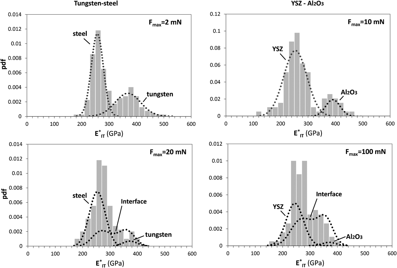
Grid CMC indentations performed on different combinations of composites (metal–metal, ceramic–ceramic, and metal–ceramic) allowed to statistically treat the results for each load level to obtain the increasing number of measured values affected by the interface. Examples of statistical distributions obtained for selected loads are shown in Fig. 8. For the sake of simplicity, the results are presented for indentation modulus only. The same findings can be obtained for hardness, but only if there is no indentation size effect for the whole load range (one must take care as the indentation size effect is generally much stronger for hardness than for indentation modulus).
Histograms and probability density functions of indentation moduli measured and identified in tungsten-steel and YSZ–Al2O3 composites at different loads. At low loads the data were fitted by bimodal Gaussian distribution, at higher loads the term of conditional probability of indentation near the interface was included in the identification procedure.

It can be seen in Fig. 8 that the peaks of indentation moduli distribution are mutually shifted to one another as the indentation load (and/or depth of penetration) increases. It is obvious that indentation at significantly higher loads would lead only to averaged values of both phases.
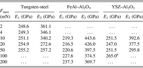
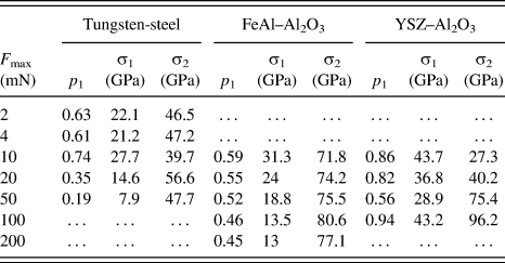
First, the data were fitted by a Gaussian bimodal distribution [Eq. (5)] using maximum likelihood method. Mean value of indentation moduli obtained by Gaussian bimodal fit for different indentation loads are listed in Table II. Using Gaussian bimodal fit, Young's modulus of the softer phase is increasingly overestimated and the harder phase value is progressively underestimated. No clear trend could be seen in the identified volume fractions and the scatters associated with both phases (Table III), which is due to the fact that variation of these parameters only adjusts Gaussian bimodal distribution to non-Gaussian data (to obtain the best fit).
Plain strain indentation moduli of individual phases identified using Gaussian bimodal fit at different loads.
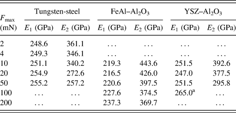
a In this case the identification converged practically to unimodal (one phase) distribution.
Phase volume fractions and scatters of plain strain indentation moduli identified using Gaussian bimodal fit at different loads.
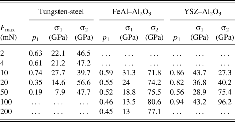
To overcome this drawback, the probability of indentation near the interface between phase 1 with actual material property 1 and phase 2 with actual material property 2 must be taken into account. Analyses performed in previous paragraphs reduced the number of additional parameters in Eq. (6) to one extra parameter only (volume/area fraction affected by the presence of the interface p
3)—see Eq. (16). However, the identification of intrinsic material properties using statistical distribution given by Eq. (6) is complicated due to the local minima problem especially in the case when the peaks in the histogram are significantly approaching (overlapping) due to the presence of indentations affected by the interface. The identification procedure was therefore carried out with additional constraints. Data measured at least at two different loads (with expected increasing proportion of volume/area fraction affected by the presence of the interface p
3) had to be included in the combined set, mean values (
 ${\overline E _1}$
,
 ${\overline E _2}$
) were restricted to be the same for whole data set, other parameters (scatters σ1, σ2 and phase volume fractions p
1, p
2, including the volume/area fraction affected by the presence of the interface p
3) were left free for each load level. Data fitting was performed using maximum likelihood method.
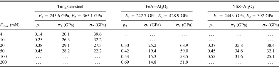
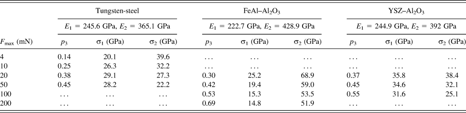
Results of the identification on the data set in which the data measured on the lowest indentation load were omitted can be seen in Table IV. Presence of the term taking into account the probability of indentation near the interface led to decrease of scatters associated with both phases and to the identified values of indentation modulus consistent with the values of pure phases and probably better than those obtained by Gaussian bimodal fit for lowest indentation load. Indentation modulus measured in “pure” tungsten is sufficiently far from the interface [Fig. 6(a)] was also lower than the expected value (Young's modulus of tungsten about ∼400 GPa (Ref. Reference Lassner and Schubert23) yields the plain strain indentation modulus of ∼440 GPa), probably due to the supplied powder quality (see Ref. Reference Brožek, Ctibor, Matějíček, Mušálek and Weiss24). Indentation moduli obtained in other phases (steel, FeAl, Al2O3, YSZ) were in a good agreement with tabulated data: Young's moduli of steel or FeAl in order of 200–210 GPa yield the plain strain indentation moduli of 220–235 GPa, Young's moduli of Al2O3 can be found in the range from 345 to 415 GPa, Reference Shackelford and Alexander25 which corresponds to the range of plain strain indentation moduli from 360 to 435 GPa, Young's modulus of YSZ ∼200 GPa (Ref. Reference Shackelford and Alexander25) yields the plain strain indentation modulus of 220 GPa.
Plain strain indentation moduli of individual phases identified on combined data set taking into account the conditional probability of indentation near the interface; volume fractions affected by the presence of the interface and scatters obtained for different load levels.
The methodology can also be applied on a material containing relatively small particles, i.e., the case when measuring in the particles is very probably affected by the surrounding matrix. Several attempts have already been made to extract the properties of thin films Reference Doerner and Nix1,Reference Menčík, Munz, Quandt, Weppelmann and Swain2 or hard particles embedded in soft matrix. Reference Durst, Göken and Vehoff9,Reference Leisen, Kerkamm, Bohn and Kamlah26 These methods were generally based on the use of an exponential function to fit the indentation modulus measured at different indentation depths Reference Doerner and Nix1,Reference Menčík, Munz, Quandt, Weppelmann and Swain2 or results obtained by FEM simulations. Reference Durst, Göken and Vehoff9,Reference Leisen, Kerkamm, Bohn and Kamlah26 Taking into account the presented configuration of the indentation across a particle (in comparison with e.g., soft to hard or hard to soft transition when indenting thin film), the use of inverse beta distribution in combination with the grid indentation technique can be regarded as an extension of these methods.
V. CONCLUDING REMARKS
The influence of presence of an interface on the distribution of measured indentation modulus was characterized in metal–metal, ceramic–ceramic, and metal–ceramic composites prepared from pairs of pure powders by spark plasma sintering. The results can be summarized as follows:
-
(1) Determination of the individual phase properties from the measured grid indentation data using standard bimodal Gaussian fit leads to the softer phase indentation modulus overestimation together with the underestimation of the harder phase values due to the presence of boundary-affected results.
-
(2) The indentation in proximity of the interface cannot always be completely avoided—the position of some indents can coincide with the phase boundary, or the invisible phase boundary can be hidden close below the indenter contact area.
-
(3) To overcome this problem, the conditional probability of indentation near the interface between phase 1 (with actual material property 1) and phase 2 (with actual material property 2) has to be taken into account.
-
(4) The change of Young's (apparent) modulus measured by indentation across the interface can be well approximated by symmetrical inverse beta distribution. The parameters of beta distribution are connected with the area/volume fraction in which the indentation measurements are affected by the interface.
-
(5) Distribution incorporating conditional probability of indentation near the interface via beta distribution leads to values of identified Young's modulus much more consistent with the values of pure phases.
ACKNOWLEDGMENT
This work was carried out in the frame of the research project 14-36566 G (Czech Science Foundation).