2 Formulation and numerical method

The governing equations are described in the context of the finite-difference/front-tracking method. The flow equations are solved in their dimensional forms but the results are presented in terms of non-dimensional quantities. The dimensional quantities are denoted by superscript $^{\ast }$ . We consider a liquid plug moving through a liquid-lined airway of radius $R^{\ast }$ as shown in figure 1. The flow is assumed to be incompressible and symmetric about the axis of the tube, and the gas and liquid phases are Newtonian fluids. Using a one-field formulation of Unverdi & Tryggvason (Reference Unverdi and Tryggvason1992), the incompressible flow equations can be written for the entire computational domain as

(2.1) $$\begin{eqnarray}\displaystyle {\displaystyle \frac{\unicode[STIX]{x2202}\unicode[STIX]{x1D70C}^{\ast }\boldsymbol{u}^{\ast }}{\unicode[STIX]{x2202}t^{\ast }}}+\unicode[STIX]{x1D735}^{\ast }\boldsymbol{\cdot }(\unicode[STIX]{x1D70C}^{\ast }\boldsymbol{u}^{\ast }\boldsymbol{u}^{\ast }) & = & \displaystyle -\unicode[STIX]{x1D735}^{\ast }p^{\ast }+\unicode[STIX]{x1D735}^{\ast }\boldsymbol{\cdot }\unicode[STIX]{x1D707}^{\ast }(\unicode[STIX]{x1D735}^{\ast }\boldsymbol{u}^{\ast }+\unicode[STIX]{x1D735}^{\ast }\boldsymbol{u}^{\ast \text{T}})\nonumber\\ \displaystyle & & \displaystyle +\,\int _{A^{\ast }}(\unicode[STIX]{x1D70E}^{\ast }(\unicode[STIX]{x1D6E4}^{\ast })\unicode[STIX]{x1D705}^{\ast }\boldsymbol{n}+\unicode[STIX]{x1D735}_{s}^{\ast }\unicode[STIX]{x1D70E}^{\ast }(\unicode[STIX]{x1D6E4}^{\ast }))\unicode[STIX]{x1D6FF}(\boldsymbol{x}^{\ast }-\boldsymbol{x}_{f})\,\text{d}A^{\ast },\qquad\end{eqnarray}$$

where $t^{\ast }$ is the time, $\boldsymbol{u}^{\ast }$ is the velocity vector, $p^{\ast }$ is the pressure field, $\unicode[STIX]{x1D70C}^{\ast }$ and $\unicode[STIX]{x1D707}^{\ast }$ are the discontinuous density and viscosity fields, respectively, and $A^{\ast }$ is the surface area. The last term on the right-hand side represents the body force due to the surface tension, where $\unicode[STIX]{x1D70E}^{\ast }$ is the surface tension coefficient that is a function of the interfacial surfactant concentration $\unicode[STIX]{x1D6E4}^{\ast }$ , $\unicode[STIX]{x1D705}^{\ast }$ is twice the mean curvature of the interface, $\boldsymbol{n}$ is a unit vector normal to the interface and $\unicode[STIX]{x1D735}_{s}^{\ast }$ is the gradient operator along the interface defined as

(2.2) $$\begin{eqnarray}\unicode[STIX]{x1D735}_{s}^{\ast }=\unicode[STIX]{x1D735}^{\ast }-\boldsymbol{n}(\boldsymbol{n}\boldsymbol{\cdot }\unicode[STIX]{x1D735}^{\ast }).\end{eqnarray}$$

The surface tension only acts on the interface as indicated by the three-dimensional Dirac delta function $\unicode[STIX]{x1D6FF}$ whose arguments $\boldsymbol{x}^{\ast }$ and $\boldsymbol{x}_{f}^{\ast }$ are the point at which the equation is evaluated and the point at the interface, respectively. The treatment of surface force as a body force was pioneered by Peskin (Reference Peskin1977) with the immersed boundary approach. The Navier–Stokes equations are supplemented by the incompressibility condition

(2.3) $$\begin{eqnarray}\unicode[STIX]{x1D735}^{\ast }\boldsymbol{\cdot }\boldsymbol{u}^{\ast }=0.\end{eqnarray}$$

We also assume that the material properties remain constant following a fluid particle:

(2.4a-c ) $$\begin{eqnarray}{\displaystyle \frac{\text{D}\unicode[STIX]{x1D70C}^{\ast }}{\text{D}t^{\ast }}}=0,\quad {\displaystyle \frac{\text{D}\unicode[STIX]{x1D707}^{\ast }}{\text{D}t^{\ast }}}=0,\quad {\displaystyle \frac{\text{D}D_{c}^{\ast }}{\text{D}t^{\ast }}}=0,\end{eqnarray}$$

where $D_{c}^{\ast }$ is the molecular diffusivity of bulk surfactant concentration and $\text{D}/\text{D}t^{\ast }=(\unicode[STIX]{x2202}/\unicode[STIX]{x2202}t^{\ast })+\boldsymbol{u}^{\ast }\boldsymbol{\cdot }\unicode[STIX]{x1D735}^{\ast }$ is the material derivative. The density and viscosity vary discontinuously across the fluid interface and are given by

(2.5a,b ) $$\begin{eqnarray}\unicode[STIX]{x1D70C}^{\ast }=\unicode[STIX]{x1D70C}_{g}^{\ast }I+\unicode[STIX]{x1D70C}_{l}^{\ast }(1-I),\quad \unicode[STIX]{x1D707}^{\ast }=\unicode[STIX]{x1D707}_{g}^{\ast }I+\unicode[STIX]{x1D707}_{l}^{\ast }(1-I),\end{eqnarray}$$

where the subscripts ‘ $g$ ’ and ‘ $l$ ’ denote properties of the gas phase and the liquid phase, respectively, and $I$ is the indicator function defined as

(2.6) $$\begin{eqnarray}I(\boldsymbol{x}^{\ast },t^{\ast })=\left\{\begin{array}{@{}ll@{}}1\quad & \text{in gas phase,}\\ 0\quad & \text{in liquid phase.}\end{array}\right.\end{eqnarray}$$

The interfacial surfactant concentration $\unicode[STIX]{x1D6E4}^{\ast }$ is defined as the amount of surfactant per unit surface area. In a static system, as the bulk concentration increases, the surfactant molecules are adsorbed at the interface until the interface becomes saturated with surfactant and attains the value $\unicode[STIX]{x1D6E4}^{\ast }=\unicode[STIX]{x1D6E4}_{\infty }^{\ast }$ , where $\unicode[STIX]{x1D6E4}_{\infty }^{\ast }$ is the maximum equilibrium concentration. In a dynamic system, $\unicode[STIX]{x1D6E4}^{\ast }$ can exceed $\unicode[STIX]{x1D6E4}_{\infty }^{\ast }$ in the region where the surfactant accumulates due to the surface flow. The surface tension decreases with the interfacial surfactant concentration approximately linearly for $\unicode[STIX]{x1D6E4}^{\ast }<\unicode[STIX]{x1D6E4}_{\infty }^{\ast }$ and the relationship becomes nonlinear for $\unicode[STIX]{x1D6E4}^{\ast }\geqslant \unicode[STIX]{x1D6E4}_{\infty }^{\ast }$ . Following Fujioka & Grotberg (Reference Fujioka and Grotberg2005) and Zheng, Fujioka & Grotberg (Reference Zheng, Fujioka and Grotberg2007), the surface tension coefficient is related to the interfacial surfactant concentration as

(2.7) $$\begin{eqnarray}{\displaystyle \frac{\unicode[STIX]{x1D70E}^{\ast }}{\unicode[STIX]{x1D70E}_{s}^{\ast }}}=\left\{\begin{array}{@{}ll@{}}\left(1-\unicode[STIX]{x1D6FD}{\displaystyle \frac{\unicode[STIX]{x1D6E4}^{\ast }}{\unicode[STIX]{x1D6E4}_{\infty }^{\ast }}}\right)\quad & \text{if }\unicode[STIX]{x1D6E4}^{\ast }<\unicode[STIX]{x1D6E4}_{\infty }^{\ast },\\ (1-\unicode[STIX]{x1D6FD})\exp \left[{\displaystyle \frac{\unicode[STIX]{x1D6FD}}{1-\unicode[STIX]{x1D6FD}}}\left(1-{\displaystyle \frac{\unicode[STIX]{x1D6E4}^{\ast }}{\unicode[STIX]{x1D6E4}_{\infty }^{\ast }}}\right)\right]\quad & \text{if }\unicode[STIX]{x1D6E4}^{\ast }\geqslant \unicode[STIX]{x1D6E4}_{\infty }^{\ast },\end{array}\right.\end{eqnarray}$$

where $\unicode[STIX]{x1D70E}_{s}^{\ast }$ is the surface tension of the clean interface and $\unicode[STIX]{x1D6FD}$ is the elasticity number.

The evolution equation for the interfacial surfactant concentration $\unicode[STIX]{x1D6E4}^{\ast }$ was derived by Stone (Reference Stone1990). Since the interfacial surfactant evolution equation is solved on a Lagrangian grid in the finite-difference/front-tracking framework, it is convenient to write it in the following form (Muradoglu & Tryggvason Reference Muradoglu and Tryggvason2008, Reference Muradoglu and Tryggvason2014):

(2.8) $$\begin{eqnarray}{\displaystyle \frac{1}{A^{\ast }}}{\displaystyle \frac{\text{D}\unicode[STIX]{x1D6E4}^{\ast }A^{\ast }}{\text{D}t^{\ast }}}=D_{s}^{\ast }\unicode[STIX]{x1D6FB}_{s}^{\ast 2}\unicode[STIX]{x1D6E4}^{\ast }+{\dot{S}}_{\unicode[STIX]{x1D6E4}}^{\ast },\end{eqnarray}$$

where $A^{\ast }$ is the area of an element of the interface, $D_{s}^{\ast }$ is the diffusion coefficient along the interface and ${\dot{S}}_{\unicode[STIX]{x1D6E4}}^{\ast }$ is the source term given by

(2.9) $$\begin{eqnarray}{\dot{S}}_{\unicode[STIX]{x1D6E4}}^{\ast }=\left\{\begin{array}{@{}ll@{}}k_{a}^{\ast }C_{s}^{\ast }(\unicode[STIX]{x1D6E4}_{\infty }^{\ast }-\unicode[STIX]{x1D6E4}^{\ast })-k_{d}^{\ast }\unicode[STIX]{x1D6E4}^{\ast }\quad & \text{if }\unicode[STIX]{x1D6E4}^{\ast }<\unicode[STIX]{x1D6E4}_{\infty }^{\ast },\\ -k_{d}^{\ast }\unicode[STIX]{x1D6E4}^{\ast }\quad & \text{if }\unicode[STIX]{x1D6E4}^{\ast }\geqslant \unicode[STIX]{x1D6E4}_{\infty }^{\ast },\end{array}\right.\end{eqnarray}$$

where $k_{a}^{\ast }$ and $k_{d}^{\ast }$ are the adsorption and the desorption coefficients, respectively, and $C_{s}^{\ast }$ is the surfactant concentration in the liquid immediately adjacent to the interface. The bulk surfactant concentration $C^{\ast }$ is governed by the advection–diffusion equation

(2.10) $$\begin{eqnarray}{\displaystyle \frac{\unicode[STIX]{x2202}C^{\ast }}{\unicode[STIX]{x2202}t^{\ast }}}+\unicode[STIX]{x1D735}^{\ast }\boldsymbol{\cdot }(C^{\ast }\boldsymbol{u}^{\ast })=\unicode[STIX]{x1D735}^{\ast }\boldsymbol{\cdot }(D_{co}^{\ast }\unicode[STIX]{x1D735}^{\ast }C^{\ast }),\end{eqnarray}$$

where $D_{co}^{\ast }$ is related to the molecular diffusion coefficient $D_{c}^{\ast }$ through the indicator function as

(2.11) $$\begin{eqnarray}D_{co}^{\ast }=D_{c}^{\ast }(1-I).\end{eqnarray}$$

The source in (2.8) is related to the bulk concentration as

(2.12) $$\begin{eqnarray}{\dot{S}}_{\unicode[STIX]{x1D6E4}}^{\ast }=-D_{co}^{\ast }(\boldsymbol{n}\boldsymbol{\cdot }\unicode[STIX]{x1D735}^{\ast }C^{\ast }|_{interface}).\end{eqnarray}$$

The adsorption layer concept developed by Muradoglu & Tryggvason (Reference Muradoglu and Tryggvason2008) is used to treat mass boundary condition at the interface. The method assumes that all the mass transfer between the interface and the bulk takes place in a thin adsorption layer adjacent to the interface. In this approach, the total amount of mass adsorbed on the interface is distributed over the adsorption layer and added to the bulk concentration evolution equation as a negative source term in a conservative manner. Equation (2.10) thus becomes

(2.13) $$\begin{eqnarray}{\displaystyle \frac{\unicode[STIX]{x2202}C^{\ast }}{\unicode[STIX]{x2202}t^{\ast }}}+\unicode[STIX]{x1D735}^{\ast }\boldsymbol{\cdot }(C^{\ast }\boldsymbol{u}^{\ast })=\unicode[STIX]{x1D735}^{\ast }\boldsymbol{\cdot }(D_{co}^{\ast }\unicode[STIX]{x1D735}^{\ast }C^{\ast })+{\dot{S}}_{c}^{\ast },\end{eqnarray}$$

where ${\dot{S}}_{c}^{\ast }$ is the source term evaluated at the interface and distributed conservatively onto the adsorption layer. With this formulation, all the mass of the bulk surfactant to be adsorbed by the interface is already consumed in the adsorption layer before the interface. Hence, the boundary condition at the interface simplifies to be $\boldsymbol{n}\boldsymbol{\cdot }\unicode[STIX]{x1D735}^{\ast }C^{\ast }|_{interface}=0$ . This approach is easy to implement and has been found to result in a better mass conservation as compared to directly imposing the boundary condition (i.e. (2.12)) at the interface boundary (Irfan & Muradoglu Reference Irfan and Muradoglu2017).

The flow equations (2.1) and (2.3) are solved fully coupled with the interfacial (2.8) and bulk (2.13) concentration evolution equations using the finite-difference/front-tracking method (Muradoglu & Tryggvason Reference Muradoglu and Tryggvason2008, Reference Muradoglu and Tryggvason2014). The spatial derivatives are discretized using second-order central differences except for the convective term in the bulk surfactant evolution equation for which a fifth-order WENO-Z scheme (Borges et al. Reference Borges, Carmona, Costa and Don2013) is used. A projection method (Harlow & Welch Reference Harlow and Welch1965; Unverdi & Tryggvason Reference Unverdi and Tryggvason1992) is used to solve the discretized equations on a stationary, staggered Eulerian grid. The numerical method is overall second- and first-order accurate in space and time, respectively. Note that it is straightforward to make the numerical method second-order accurate in time but the time-stepping error is generally found to be negligibly small compared to the spatial error mainly due to the small time step imposed by the stability requirements.

The liquid–gas interface is tracked using a separate Lagrangian grid which consists of linked marker points (the front) moving with the local flow velocity interpolated from the stationary Eulerian grid. The piece of the Lagrangian grid between two marker points is called a front element. The interfacial surfactant concentration equation, (2.8), is solved on the Lagrangian grid using second-order centred differences for the spatial derivatives and a first-order Euler method for the time integration. The Lagrangian grid is also used to calculate the surface tension, which is then distributed onto the Eulerian grid points near the interface by using Peskin’s cosine distribution function (Peskin Reference Peskin1977), and added to the momentum equations as a body force as described by Tryggvason et al. (Reference Tryggvason, Bunner, Esmaeeli, Juric, Al-Rawahi, Tauber, Han, Nas and Jan2001).

The indicator function is computed at each time step based on the location of the interface using the standard procedure (Tryggvason et al. Reference Tryggvason, Bunner, Esmaeeli, Juric, Al-Rawahi, Tauber, Han, Nas and Jan2001) and is used to set the fluid properties in the liquid and gas phases. It is also utilized to compute the bulk surfactant concentration near the interface and to distribute the surfactant source terms onto the Eulerian grid in the adsorption layer (Muradoglu & Tryggvason Reference Muradoglu and Tryggvason2008).

The Lagrangian grid is restructured at every time step by deleting the front elements that are smaller than a prespecified lower limit and by splitting the front elements that are larger than a prespecified upper limit in the same way as described by Tryggvason et al. (Reference Tryggvason, Bunner, Esmaeeli, Juric, Al-Rawahi, Tauber, Han, Nas and Jan2001) to keep the front element size nearly uniform and comparable to the background Eulerian grid size. Restructuring the Lagrangian grid is crucial since it avoids unresolved wiggles due to small elements and lack of resolution due to large elements. Note that restructuring the Lagrangian grid is performed such that the mass conservation is strictly satisfied for the surfactant at the interface (Muradoglu & Tryggvason Reference Muradoglu and Tryggvason2008).

Unlike some other one-field approaches such as volume-of-fluid and level-set methods, the topological changes due to breakup and coalescence are not handled automatically in the front-tracking method (see e.g. Tryggvason, Scardovelli & Zaleski Reference Tryggvason, Scardovelli and Zaleski2011). Although it is possible to make it automated using the indicator function (Shin & Juric Reference Shin and Juric2002), we adopt a simpler procedure developed by Olgac, Kayaalp & Muradoglu (Reference Olgac, Kayaalp and Muradoglu2006) and assume that the liquid plug ruptures when the distance between the leading and trailing air fingers is smaller than a prespecified threshold value, $l_{th}$ . For this purpose, the distance between air fingers at the centreline is monitored during the simulations and when the distance becomes smaller than $\ell _{th}$ , the front element that is closest to the centreline on each air finger is deleted and then a new element is created to merge two air fingers by connecting the hanging marker points. In the present study, the threshold value is taken as $\ell _{th}=\unicode[STIX]{x0394}r$ , where $\unicode[STIX]{x0394}r$ is the grid size in the radial direction. As shown in appendix B, the results are not very sensitive to the choice of the threshold value as long as it is of the order of the grid size.

The front-tracking method was pioneered by Glimm and colleagues (Chern et al. Reference Chern, Glimm, McBryan, Plohr and Yaniv1986; Glimm et al. Reference Glimm, Graham, Grove, Li, Smith, Tan, Tangerman and Zhang1998) and readers are referred to Chern et al. (Reference Chern, Glimm, McBryan, Plohr and Yaniv1986), Glimm et al. (Reference Glimm, Graham, Grove, Li, Smith, Tan, Tangerman and Zhang1998), Unverdi & Tryggvason (Reference Unverdi and Tryggvason1992) and Tryggvason et al. (Reference Tryggvason, Bunner, Esmaeeli, Juric, Al-Rawahi, Tauber, Han, Nas and Jan2001) for the details of the method. A complete description of the treatment of the soluble surfactant can be found in Muradoglu & Tryggvason (Reference Muradoglu and Tryggvason2008, Reference Muradoglu and Tryggvason2014) and Tasoglu, Demirci & Muradoglu (Reference Tasoglu, Demirci and Muradoglu2008). The method has been rigorously validated and successfully used to study various flows involving thin films similar to the problem considered in this paper; see, for instance, Muradoglu & Stone (Reference Muradoglu and Stone2007) and Olgac & Muradoglu (Reference Olgac and Muradoglu2013a ,Reference Olgac and Muradoglu b ). The method is also validated for clean plug propagation and rupture and the results are presented in appendix A.

3 Problem statement

The physical problem is sketched in figure 1. The flow is assumed to be symmetric about the axis of the channel so the computational domain has dimensions of $R^{\ast }$ in the radial direction and $L_{z}^{\ast }$ in the axial direction. Flow is initially quiescent and the liquid plug is driven by an applied pressure difference between the front and the rear air fingers, $\unicode[STIX]{x0394}p^{\ast }=p_{1}^{\ast }-p_{2}^{\ast }$ . The plug is initially located at the airway centreline close to the inlet section with an initial length of $L_{pi}^{\ast }$ . The precursor and trailing liquid film thicknesses far from the plug are denoted as $h_{2}^{\ast }$ and $h_{1}^{\ast }$ , respectively, and they are initially set to be equal. The initial plug shape is approximated by hemispheres of radii of $R^{\ast }-h_{2}^{\ast }$ and $R^{\ast }-h_{1}^{\ast }$ for the front and rear menisci, respectively. No-slip boundary conditions are applied at the tube wall. The initial surfactant concentration in the liquid is prescribed to be $C_{0}^{\ast }$ and the interfacial surfactant concentration is initially in equilibrium with $C_{0}^{\ast }$ . At the precursor film far ahead of the plug, the bulk surfactant concentration is fixed to be $C_{0}^{\ast }$ .

The governing equations are solved in their dimensional forms but the results are presented in terms of relevant non-dimensional quantities. Following Fujioka & Grotberg (Reference Fujioka and Grotberg2005), the quantities are non-dimensionalized using the length scale ${\mathcal{L}}^{\ast }=R^{\ast }$ , the time scale ${\mathcal{T}}^{\ast }=\unicode[STIX]{x1D707}_{l}^{\ast }R^{\ast }/\unicode[STIX]{x1D70E}_{s}^{\ast }$ and the velocity scale ${\mathcal{V}}^{\ast }={\mathcal{L}}^{\ast }/{\mathcal{T}}^{\ast }=\unicode[STIX]{x1D70E}_{s}^{\ast }/\unicode[STIX]{x1D707}_{l}^{\ast }$ . Thus the non-dimensional velocity vector, pressure, bulk surfactant concentration and interfacial surfactant concentration are defined as $\boldsymbol{u}=\boldsymbol{u}^{\ast }/(\unicode[STIX]{x1D70E}_{s}^{\ast }/\unicode[STIX]{x1D707}_{l}^{\ast })$ , $p=p^{\ast }/(\unicode[STIX]{x1D70E}_{s}^{\ast }/R^{\ast })$ , $C=C^{\ast }/C_{cmc}^{\ast }$ and $\unicode[STIX]{x1D6E4}=\unicode[STIX]{x1D6E4}^{\ast }/\unicode[STIX]{x1D6E4}_{\infty }^{\ast }$ , respectively. Note that $C_{cmc}^{\ast }$ is the critical micelle concentration. The relevant non-dimensional numbers are then defined as

(3.1) $$\begin{eqnarray}\left.\begin{array}{@{}c@{}}\unicode[STIX]{x1D706}=\unicode[STIX]{x1D70C}_{l}^{\ast }\unicode[STIX]{x1D70E}_{s}^{\ast }R^{\ast }/\unicode[STIX]{x1D707}_{l}^{\ast 2},\quad \unicode[STIX]{x1D712}=\unicode[STIX]{x1D6E4}_{\infty }^{\ast }/(C_{cmc}^{\ast }R^{\ast }),\quad Sc=\unicode[STIX]{x1D707}_{l}^{\ast }/(\unicode[STIX]{x1D70C}_{l}^{\ast }D_{l}^{\ast }),\quad Sc_{s}=\unicode[STIX]{x1D707}_{l}^{\ast }/(\unicode[STIX]{x1D70C}_{l}^{\ast }D_{s}^{\ast }),\\ K_{a}=k_{a}^{\ast }C_{cmc}^{\ast }R^{\ast 2}/D_{s}^{\ast },\quad K_{d}=k_{d}^{\ast }R^{\ast 2}/D_{s}^{\ast },\quad L_{pi}=L_{p}^{\ast }/R^{\ast },\quad \unicode[STIX]{x0394}p=(p_{1}^{\ast }-p_{2}^{\ast })R^{\ast }/\unicode[STIX]{x1D70E}_{s}^{\ast },\end{array}\right\}\qquad\end{eqnarray}$$

where $\unicode[STIX]{x1D706}$ is the Laplace number, $\unicode[STIX]{x1D712}$ is the dimensionless adsorption depth, $Sc$ and $Sc_{s}$ are the bulk and interfacial Schmidt numbers, respectively, $K_{a}$ and $K_{d}$ are the dimensionless adsorption and desorption coefficients, respectively, $L_{pi}$ is the non-dimensional initial distance between the leading and trailing air fingers and $\unicode[STIX]{x0394}p$ is the dimensionless applied pressure difference.

Our study is focused on modelling plug rupture and airway reopening in adult human lungs. This phenomenon is prominent in surface-tension-dominated flows, i.e. when the airway radius is small enough. Owing to the bifurcation of bronchi and bronchioles, which reduce their radii each time as the airway splits, the required conditions are met from the seventh or eighth generation on, where the gravitational effects become negligible. Following Crystal (Reference Crystal1997), we assume $R^{\ast }\in [0.05,0.1]~\text{cm}$ as a typical range for the airway size of an adult lung airway at ninth to tenth generation. Another assumption of our model consists in positing that the bilayer liquid, which lines the airway wall and is formed by mucus and serous, can be conceptually homogenized in a Newtonian fluid with intermediate properties. This approach has recently been followed by Tai et al. (Reference Tai, Bian, Halpern, Zheng, Filoche and Grotberg2011), who took $\unicode[STIX]{x1D707}_{l}^{\ast }=0.13~\text{poise}$ , $\unicode[STIX]{x1D70C}_{l}^{\ast }=1~\text{g}~\text{m}^{-3}$ and $\unicode[STIX]{x1D70E}_{s}^{\ast }=20~\text{dyn}~\text{cm}^{-1}$ . The resulting Laplace number is $\unicode[STIX]{x1D706}=O(100)$ . We thus assume $\unicode[STIX]{x1D706}=100$ as the reference value.

For the pulmonary surfactants, the adsorption and the desorption kinetics are $k_{a}^{\ast }\approx 1.7\times 10^{3}~\text{cm}^{3}~\text{g}^{-1}~\text{s}^{-1}$ and $k_{d}^{\ast }\approx 1.7\times 10^{-2}~\text{s}^{-1}$ (Launois-Surpas et al. Reference Launois-Surpas, Ivanova, Panaiotov, Proust, Puisieux and Georgiev1992; Otis et al. Reference Otis, Ingenito, Kamm and Johnson1994), whereas the critical micelle bulk concentration $C_{cmc}^{\ast }\approx 10^{-3}~\text{g}~\text{cm}^{-3}$ . Agrawal & Neuman (Reference Agrawal and Neuman1988) measured the surface diffusivity of pulmonary surfactants as $D_{s}^{\ast }\in [1\times 10^{-7},7\times 10^{-7}]~\text{cm}^{2}~\text{s}^{-1}$ . Based on these values, the reference non-dimensional absorption and desorption rates are set to $K_{a}=10^{4}$ and $K_{d}=10^{2}$ . The maximum equilibrium interfacial concentration has been estimated by Schurch et al. (Reference Schurch, Bachofen, Goerke and Possmayer1989) for the pulmonary surfactants to be $\unicode[STIX]{x1D6E4}_{\infty }^{\ast }\approx 3.1\times 10^{-7}~\text{g}~\text{cm}^{-2}$ . Using this value as a reference, we predict the dimensionless adsorption depth to be $\unicode[STIX]{x1D712}\approx 0.01$ . Finally, we assume the elasticity number $\unicode[STIX]{x1D6FD}=0.7$ (Otis et al. Reference Otis, Ingenito, Kamm and Johnson1994) and the Schmidt numbers $Sc_{s}=100$ and $Sc=10$ (Fujioka & Grotberg Reference Fujioka and Grotberg2005).

The effects of the surface viscosity and the disjoining pressure are not taken into account in the present study. The surface viscosity for the lung surfactant was measured by Meban (Reference Meban1978) to be in the range of $\unicode[STIX]{x1D707}^{s}=2\times 10^{-7}$ – $2.2\times 10^{-5}~\text{kg}~\text{s}^{-1}$ . More recently, Rudiger et al. (Reference Rudiger, Tolle, Meier and Rustow2005) reported that the surface viscosity of natural lung surfactant preparations is below $\unicode[STIX]{x1D707}^{s}\sim 5\times 10^{-6}~\text{kg}~\text{s}^{-1}$ , except for Survanta for which the surface viscosity varies greatly and can increase up to $\unicode[STIX]{x1D707}^{s}\sim 18\times 10^{-6}~\text{kg}~\text{s}^{-1}$ in very high concentrations. For $R^{\ast }=10^{-3}~\text{m}$ , the Boussinesq number ( $Bq=\unicode[STIX]{x1D707}^{s}/\unicode[STIX]{x1D707}_{l}R^{\ast }$ ) can be estimated to be in the range of $0.2<Bq<22$ . More recently, Zell et al. (Reference Zell, Nowbahar, Mansard, Leala, Deshmukh, Mecca, Tucker and Squires2014) have shown that the actual values of surface viscosity for common surfactants are actually several orders of magnitude smaller than those measured earlier, which suggests that it is reasonable to assume $Bq<1$ . Thus the effects of surface viscosity are expected to be minor as discussed recently by Gounley et al. (Reference Gounley, Boedec, Jaeger and Leonetti2016). We finally note that an extremely fine grid is required to resolve the effects of disjoining pressure, which is computationally infeasible even in the present axisymmetric simulations.

The elastic nature of airways is another mechanical property neglected in the present study. The entire airway tree consists of elastic tubes that become increasingly more flexible and compliant in the lower generations (Halpern & Grotberg Reference Halpern and Grotberg1992; Grotberg Reference Grotberg2011; Heil & Hazel Reference Heil and Hazel2011). The relative importance of the airway wall elasticity can be characterized by $\unicode[STIX]{x1D6E4}_{HH}=\unicode[STIX]{x1D70E}_{s}^{\ast }/R^{\ast }K^{\ast }$ , where $K^{\ast }=E^{\ast }/12(1-\unicode[STIX]{x1D708}^{2})(h_{w}^{\ast }/R^{\ast })^{3}$ is the flexural rigidity with $E^{\ast }$ , $\unicode[STIX]{x1D708}$ and $h_{w}^{\ast }$ being Young’s modulus, Poisson’s ratio and the thickness of the airway wall, respectively (Hazel & Heil Reference Hazel and Heil2003). This parameter represents the ratio of the surface tension forces to the bending stiffness of the airway wall. Following Halpern & Grotberg (Reference Halpern and Grotberg1992), the dimensional values for the ninth to tenth generation can be specified as $R^{\ast }=5\times 10^{-2}~\text{cm}$ , $E^{\ast }=6\times 10^{4}~\text{dyn}~\text{cm}^{-2}$ , $h_{w}^{\ast }=2.5\times 10^{-3}~\text{cm}$ and $\unicode[STIX]{x1D708}=0.5$ , which yields $\unicode[STIX]{x1D6E4}_{HH}=480\gg 1$ . As seen, the elasticity of the airway wall and resulting fluid–structure interactions are likely to be significant and need to be taken into account for more accurate modelling of pulmonary flow in the generations considered in the present study. Note that Halpern & Grotberg (Reference Halpern and Grotberg1992) define another non-dimensional parameter, $\unicode[STIX]{x1D6E4}_{HG}=(1-\unicode[STIX]{x1D708}^{2})\unicode[STIX]{x1D70E}_{s}^{\ast }/E^{\ast }h_{w}^{\ast }$ , which represents the ratio of surface-tension forces to elastic forces and is related to $\unicode[STIX]{x1D6E4}_{HH}$ as $\unicode[STIX]{x1D6E4}_{HG}=(1/12)(h_{w}^{\ast }/R^{\ast })^{2}\unicode[STIX]{x1D6E4}_{HH}$ . Using the same dimensional values, we obtain $\unicode[STIX]{x1D6E4}_{HG}=0.1$ confirming the significance of the tube elasticity.

4 Results and discussion

In this section, simulations are performed to examine the effects of surfactant on liquid plug propagation and rupture dynamics. All the computations are performed using tensor-product structured grids that are uniform in the axial direction and slightly stretched in the radial direction in order to better resolve the liquid film regions between the tube wall and air fingers. The stretching is done in such a way that the radial grid size, $\unicode[STIX]{x0394}r$ , is two times larger at the centreline than that at the tube wall. The computational domain extends $L_{z}^{\ast }=20R^{\ast }$ in the axial direction and the centre of the liquid plug is initially located at $z_{c}^{\ast }=2.95R^{\ast }$ . The present numerical method is validated against the previous computational studies of Fujioka et al. (Reference Fujioka, Takayama and Grotberg2008) and Hassan et al. (Reference Hassan, Uzgoren, Fujioka, Grotberg and Shyy2011) for a surfactant-free liquid plug propagation without and with a rupture, respectively. As discussed in appendix A, the present results are found to be in good agreement with the previous simulations performed using different numerical techniques. A comprehensive grid convergence study is also conducted to determine the minimum grid size to obtain grid-independent solutions. As detailed in appendix B, a grid resolution containing 96 cells in the radial direction is found to be sufficient to reduce the spatial discretization error below 3 %. Therefore this grid resolution is used in all the simulations presented here.

Figure 2.

Time evolution of interfacial (left-hand part of each panel) and bulk (right-hand part of each panel) surfactant concentration for $C_{0}=5\times 10^{-5}$ . Snapshots are taken at times $t=$ (a) 49.33, (b) 202.39, (c) 240.90, (d) 241.47, (e) 242.10 and (f) 273.85. The dashed lines show the surface velocity of the interface. The surface velocity is computed with respect to the tip of the leading air finger before rupture (a–c). The intersection of the dashed lines with the interface indicates the stagnation points. ( $L_{pi}=1.0$ , $\unicode[STIX]{x0394}p=1$ , $\unicode[STIX]{x1D706}=100$ , $\unicode[STIX]{x1D6FD}=0.7$ , $\unicode[STIX]{x1D712}=0.01$ , $Sc=10$ , $Sc_{s}=100$ , $K_{a}=10^{4}$ , $K_{d}=100$ .)

Figure 3.

Time evolution of interface and pressure contours for a clean (left-hand side of each panel) and a contaminated (right-hand side of each panel) plug. Snapshots are taken at times $t-t_{rupture}=$ (a) $-167.62$ , (b) $-36.70$ , (c) 0, (d) 0.55, (e) 1.15, (f) 1.81, (g) 3.71, (h) 10.10 and (i) 39.19, where $t_{rupture}$ is the rupture time, which is 218.28 and 240.92 for the clean and contaminated cases, respectively. The dashed black lines show the surface velocity of the interface. The surface velocity is computed with respect to the tip of the leading air finger before the rupture (a–c). The intersection of the dashed lines with the interface indicates the stagnation points. The non-dimensional parameters are $L_{pi}=1.0$ , $\unicode[STIX]{x0394}p=1$ , $\unicode[STIX]{x1D706}=100$ for both the clean and the contaminated cases. The other parameters for the contaminated case are $C_{0}=5\times 10^{-5}$ , $\unicode[STIX]{x1D6FD}=0.7$ , $\unicode[STIX]{x1D712}=0.01$ , $Sc=10$ , $Sc_{s}=100$ , $K_{a}=10^{4}$ , $K_{d}=100$ .

Figure 4.

The combined effects of the bulk surfactant concentration and the liquid film thickness. Time evolution of (a) plug length ( $Lp$ ), (b) maximum difference in wall pressure ( $P_{max}-P_{min}$ ), (c) minimum wall pressure ( $P_{min}$ ) and (d) maximum difference in wall shear stress ( $\unicode[STIX]{x1D70F}_{max}-\unicode[STIX]{x1D70F}_{min}$ ) is plotted for liquid film thickness of $h_{2}=0.05$ and $h_{2}=0.07$ , and for $C_{0}=0$ (clean) and $C_{0}=5\times 10^{-5}$ (contaminated) cases. ( $L_{pi}=1.0$ , $\unicode[STIX]{x0394}p=1$ , $\unicode[STIX]{x1D706}=100$ , $\unicode[STIX]{x1D6FD}=0.7$ , $\unicode[STIX]{x1D712}=0.01$ , $Sc=10$ , $Sc_{s}=100$ , $K_{a}=10^{4}$ , $K_{d}=100$ .)

We first designate a baseline case to facilitate a systematic examination of the effects of various flow parameters. Based on the discussions in § 3, the baseline case is defined as $\unicode[STIX]{x0394}p=1$ , $L_{pi}=1.0$ , $\unicode[STIX]{x1D706}=100$ , $\unicode[STIX]{x1D712}=0.01$ , $Sc=10$ , $Sc_{s}=100$ , $K_{a}=10^{4}$ , $K_{d}=100$ and $\unicode[STIX]{x1D6FD}=0.7$ . Only one non-dimensional parameter is varied at a time. The bulk surfactant concentration of $C_{0}=5\times 10^{-5}$ is also used as the baseline value unless specified otherwise. Simulations are first performed for the base case and the evolutions of the bulk and interfacial surfactant concentrations are shown in figure 2 before and after plug rupture at non-dimensional times of $t=49.33$ , 202.39, 240.90, 241.47, 242.10 and 273.85. This figure shows that the interfacial surfactant accumulates on the front meniscus interface with a maximum concentration located around the stagnation point at the shoulder where the mechanical stresses are expected to be maximum and prone to cause significant damage to epithelial cells (Huh et al. Reference Huh, Fujioka, Tung, Futai, Paine, Grotberg and Takayama2007). In other words, the interfacial surfactant accumulates where it is needed to protect the epithelium before and after the rupture takes place. In this figure, the surface velocity is also plotted as dashed lines to show the rigidification effect of the surfactant. Note that the surface velocity is defined as $U_{s}^{\ast }=\boldsymbol{u}_{r}^{\ast }\boldsymbol{\cdot }\boldsymbol{t}$ , where $\boldsymbol{t}$ is the unit tangent vector at the interface and $\boldsymbol{u}_{r}^{\ast }$ is the relative velocity of the interface with respect to the frame moving with the tip of the leading air finger and the laboratory frame before and after the rupture, respectively. The surface velocity is non-dimensionalized as $U_{s}=\unicode[STIX]{x1D707}_{l}^{\ast }U_{s}^{\ast }/\unicode[STIX]{x1D70E}^{\ast }$ . As seen, the surfactant-induced Marangoni stresses immobilize where the surfactant is accumulated. The interfacial surfactant also accumulates on the interface of the trailing meniscus near the centreline but with a concentration about an order of magnitude smaller compared to that on the front meniscus. The effects of the surfactant on the mechanical stresses are shown in figure 3 where the time evolutions of the constant contours of the pressure in the plug region are plotted side by side for the clean and the contaminated cases. Since the clean plug ruptures earlier, the snapshots are taken at times $t-t_{rupture}=-167.62$ , $-36.70$ , 0.0, 0.55, 1.15, 1.81, 3.71, 10.10 and 39.19, where $t_{rupture}$ is the rupture time, which is 216.41 and 238.54 for the clean and contaminated cases, respectively. This figure qualitatively shows that even a small amount of surfactant can significantly reduce the pressure on the wall, i.e. the maximum magnitude of the wall pressure is reduced as much as 15 % and 22 % before and after the rupture, respectively. In addition, the larger negative wall pressure in the clean case indicates that the surfactant-deficient airways are more prone to collapse during the plug rupture process. The surface velocities are also plotted as dashed lines in this figure. The rigidification effect of the surfactant is better seen in this figure, i.e. the interface velocity reduces in the contaminated case as the surfactant accumulates at the interface and the interface of the leading air finger becomes almost completely immobilized before the plug ruptures. The surfactant-induced rigidification of the interface is believed to be the main mechanism responsible for stabilization of the thinning film and inhibition of coalescence of interfaces (plug rupture) as discussed recently by Soligo, Roccon & Soldati (Reference Soligo, Roccon and Soldati2019).

The effects of the surfactant are quantified in figure 4 where the time evolutions of the plug length, the maximum difference in wall pressure, the minimum wall pressure and the maximum difference in wall shear stress are plotted for the clean and contaminated interfaces. Simulations are performed for precursor film thickness of $h_{2}=0.05$ and $h_{2}=0.07$ to demonstrate how the precursor film thickness influences the plug motion and rupture in the clean and contaminated cases. As seen, the plug rupture results in sudden jumps in the wall pressure and wall shear stress, and the surfactant reduces the magnitude of the mechanical stresses significantly for both values of the precursor liquid film thickness. The plug ruptures earlier and the wall pressure and wall shear stress variations become larger when the initial precursor film is thinner as also observed by Fujioka et al. (Reference Fujioka, Takayama and Grotberg2008) and Hassan et al. (Reference Hassan, Uzgoren, Fujioka, Grotberg and Shyy2011). It is also interesting to see that the surfactant generally delays the plug rupture, which indicates that excessive surfactant delays and may even prevent airway reopening, as will be discussed in detail below.

Figure 5.

Effects of bulk surfactant concentration on plug propagation and rupture in the range $C_{0}=0$ (clean) to $C_{0}=5\times 10^{-4}$ (highly contaminated). Time evolution of (a) plug length ( $L_{p}$ ), (b) maximum difference in wall pressure ( $P_{max}-P_{min}$ ) and (c) maximum difference in wall shear stress ( $\unicode[STIX]{x1D70F}_{max}-\unicode[STIX]{x1D70F}_{min}$ ). ( $L_{pi}=1.0$ , $h_{2}=0.05$ , $\unicode[STIX]{x0394}p=1$ , $\unicode[STIX]{x1D706}=100$ , $\unicode[STIX]{x1D6FD}=0.7$ , $\unicode[STIX]{x1D712}=0.01$ , $Sc=10$ , $Sc_{s}=100$ , $K_{a}=10^{4}$ , $K_{d}=100$ .)

Figure 6.

Effects of bulk surfactant concentration on (a) the interfacial surfactant concentration and Marangoni stress distributions and (b) surface velocity distribution at $t=t_{rupture}$ for $C_{0}\leqslant 2.5\times 10^{-4}$ and at $t=453.5$ for $C_{0}=5\times 10^{-4}$ . ( $L_{pi}=1.0$ , $h_{2}=0.05$ , $\unicode[STIX]{x0394}p=1$ , $\unicode[STIX]{x1D706}=100$ , $\unicode[STIX]{x1D6FD}=0.7$ , $\unicode[STIX]{x1D712}=0.01$ , $Sc=10$ , $Sc_{s}=100$ , $K_{a}=10^{4}$ , $K_{d}=100$ .)

Figure 7.

The time evolution of the minimum radius of the neck and its time derivative (‘snap velocity’) after rupture. ( $L_{pi}=1.0$ , $h_{2}=0.05$ , $\unicode[STIX]{x0394}p=1$ , $\unicode[STIX]{x1D706}=100$ , $\unicode[STIX]{x1D6FD}=0.7$ , $\unicode[STIX]{x1D712}=0.01$ , $Sc=10$ , $Sc_{s}=100$ , $K_{a}=10^{4}$ , $K_{d}=100$ .)

Figure 8.

Wall pressure and wall shear stress distributions for a clean plug ( $C_{0}=0$ ) (a,b), a mildly contaminated plug ( $C_{0}=5\times 10^{-5}$ ) (c,d) and a highly contaminated plug ( $C_{0}=10^{-4}$ ) (e,f). ( $L_{pi}=1.0$ , $h_{2}=0.05$ , $\unicode[STIX]{x0394}p=1$ , $\unicode[STIX]{x1D706}=100$ , $\unicode[STIX]{x1D6FD}=0.7$ , $\unicode[STIX]{x1D712}=0.01$ , $Sc=10$ , $Sc_{s}=100$ , $K_{a}=10^{4}$ , $K_{d}=100$ .)

Figure 9.

Effects of elasticity number on plug propagation and rupture in the range $\unicode[STIX]{x1D6FD}=0$ to $\unicode[STIX]{x1D6FD}=1.5$ . Time evolution of (a) plug length ( $L_{p}$ ), (b) maximum difference in wall pressure ( $P_{max}-P_{min}$ ) and (c) maximum difference in wall shear stress ( $\unicode[STIX]{x1D70F}_{max}-\unicode[STIX]{x1D70F}_{min}$ ). ( $L_{pi}=1.0$ , $h_{2}=0.05$ , $\unicode[STIX]{x0394}p=1$ , $\unicode[STIX]{x1D706}=100$ , $\unicode[STIX]{x1D712}=0.01$ , $Sc=10$ , $Sc_{s}=100$ , $K_{a}=10^{4}$ , $K_{d}=100$ , $C_{0}=10^{-4}$ .)

We next examine the effects of bulk surfactant concentration on plug propagation and rupture. For this purpose, simulations are performed for various bulk surfactant concentrations in the range $C_{0}=0$ (clean) to $C_{0}=5\times 10^{-4}$ (highly contaminated), and the results are shown in figures 5–7. Figure 5 shows the time evolutions of the plug length ( $L_{p}$ ), the maximum difference in the wall pressure ( $P_{max}-P_{min}$ ) and the maximum difference in the wall shear stress ( $\unicode[STIX]{x1D70F}_{max}-\unicode[STIX]{x1D70F}_{min}$ ). As seen, rupture is delayed and the mechanical stresses on the wall are reduced significantly as $C_{0}$ is increased, and rupture is prevented completely after $C_{0}\geqslant 5\times 10^{-4}$ . The distributions of the interfacial surfactant concentration ( $\unicode[STIX]{x1D6E4}$ ), the Marangoni stress ( $\unicode[STIX]{x1D70F}_{M}$ ) and the surface velocity ( $U_{s}$ ) are also plotted in figure 6 just after the plug ruptures, i.e. at $t=t_{rupture}$ with $t_{rupture}$ being the rupture time, as a function of the arclength ( $s$ ) measured from the centreline in the clockwise and counterclockwise directions for the leading and trailing fingers, respectively. Note that the arclength of the trailing air finger is made negative to distinguish it from that of the leading air finger as sketched in figure 1. When the liquid plug ruptures, a negative arclength denotes a point on the interface whose axial location $z_{p}$ is smaller than the axial location of the rupture point $z_{rupture}$ . Note that the Marangoni stress is defined as $\unicode[STIX]{x1D70F}_{M}^{\ast }=\unicode[STIX]{x2202}\unicode[STIX]{x1D70E}^{\ast }/\unicode[STIX]{x2202}s^{\ast }$ . As seen, the pressure and viscous shear stress on the tube wall are monotonically reduced when the bulk surfactant concentration is increased mainly due to accumulation of more interfacial surfactant at the rear edge of the leading air finger close to the wall. As $C_{0}$ increases, the interfacial surfactant concentration increases on both the front and the trailing meniscus interfaces but the increase is more dramatic for the front meniscus. At low concentrations, the interfacial surfactant is largely accumulated at the back shoulder of the leading air finger and the interfacial surfactant distribution gets wider and eventually covers the entire interface of the front meniscus as the bulk concentration increases. The Marangoni stresses oppose the viscous shear stresses, and thus reduce the mobility of the interface, which is known as the rigidification effect of surfactant as first explained consistently by Frumkin & Levich (Reference Frumkin and Levich1947). The immobilization effect of surfactant is shown in figure 6(b) where the interfacial surfactant concentration and surface velocity distributions are plotted for the various values of bulk surfactant concentration. As can be seen in this figure, the surface velocity decreases monotonically as $C_{0}$ increases and the meniscus interface is immobilized almost completely for $C_{0}\geqslant 2.5\times 10^{-4}$ . When the plug ruptures, the interface retracts quickly towards the airway wall. The effects of surfactant on the retraction of the interface are shown in figure 7 where the time evolutions of the minimum radius of the interface $R_{min}$ and the snap velocity $V_{snap}$ defined as $V_{snap}=\text{d}R_{min}/\text{d}t$ are plotted after the rupture. This figure shows that the surfactant does not have a significant effect on retraction when $C_{0}\leqslant 5\times 10^{-5}$ but the retraction velocity reduces slightly as $C_{0}$ is further increased. Figure 8 illustrates the variation of the wall pressure and the wall shear stress at various times before and after the plug ruptures for clean ( $C_{0}=0$ ), mildly contaminated ( $C_{0}=5\times 10^{-5}$ ) and highly contaminated ( $C_{0}=10^{-4}$ ) cases. Since plugs rupture at different axial locations, the axial coordinate is shifted by the rupture point $z_{rupture}$ to facilitate a direct comparison. As can be seen in this figure, not only the magnitudes but also the gradients of the wall pressure and wall shear stress become large especially near the leading and trailing menisci and are amplified significantly by the plug rupture. Note that the gradients of the mechanical stresses are as important as their magnitudes in potentially injuring cells (Glindmeyer, Smith & Gaver Reference Glindmeyer, Smith and Gaver2012). Figure 8 also shows that the surfactant generally reduces both magnitude and gradient of mechanical stresses on the wall and its effects are amplified as more surfactant is added to the plug liquid. These results confirm the experimental findings of Bilek et al. (Reference Bilek, Dee and Gaver2003) that flow-induced cell injuries can be abated completely by adding more surfactant into the liquid plug. However, the surfactant comes with a side effect: it also delays the plug rupture significantly implying that an excessive amount of surfactant may even prevent airway reopening. Therefore there must be a just sufficient amount of pulmonary surfactant for the best functioning of the lungs. Note that surfactant reduces the mechanical stresses by two mechanisms: (i) the Marangoni stresses due to surface tension gradient, which effectively rigidifies the interface, and (ii) the reduction in the Laplace pressure due to the reduction in surface tension, which consequently reduces the pressure in the liquid near the plug’s meniscus, as seen in figure 8.

The elasticity number may be considered as the strength of the surfactant, so it is expected to have a similar effect on plug propagation and rupture as does the bulk surfactant concentration. This is verified in figure 9 where the results are plotted for the bulk surfactant concentration of $C_{0}=10^{-4}$ and various values of the elasticity number while keeping the other parameters the same as the baseline case. Note that the bulk surfactant concentration is taken to be much larger than the baseline value in order to see significant surfactant effects even for a small value of the elasticity number. As seen in this figure, the mechanical stresses are reduced and plug rupture is delayed as the elasticity number is increased. Figure 10 shows that the interfacial surfactant is accumulated and narrowly distributed on the shoulder of the leading air finger rendering a large part of the interface nearly clean at small elasticity numbers. The distribution gets wider as the elasticity number increases and eventually covers the entire back side of the leading air finger resembling the case with an excessive bulk surfactant concentration in figure 5. The interface mobility is reduced monotonically as $\unicode[STIX]{x1D6FD}$ increases, and the interface of the leading and trailing menisci immobilizes almost completely for $\unicode[STIX]{x1D6FD}\geqslant 1$ showing the rigidification effect of surfactant.

Figure 10.

Effects of elasticity number on the interfacial surfactant concentration and surface velocity distributions at $t=t_{rupture}$ for $\unicode[STIX]{x1D6FD}\leqslant 1$ and at $t=316.2$ for $\unicode[STIX]{x1D6FD}=1.5$ . ( $L_{pi}=1.0$ , $h_{2}=0.05$ , $\unicode[STIX]{x0394}p=1$ , $\unicode[STIX]{x1D706}=100$ , $\unicode[STIX]{x1D712}=0.01$ , $Sc=10$ , $Sc_{s}=100$ , $K_{a}=10^{4}$ , $K_{d}=100$ , $C_{0}=10^{-4}$ .)

We next perform simulations to investigate the effects of the applied pressure difference, $\unicode[STIX]{x0394}p$ , and the Laplace number, $\unicode[STIX]{x1D706}$ , on the rupture dynamics for the clean and contaminated cases. The pressure difference drives the flow and determines the speed of the plug while the Laplace number accounts for the combination of inertia, tube size (curvature), surface tension and viscous effects. Thus they both influence the fluid dynamics of the plug motion and rupture. First, $\unicode[STIX]{x0394}p$ is varied in the range $\unicode[STIX]{x0394}p=0.75$ to $\unicode[STIX]{x0394}p=3$ while keeping all the other non-dimensional parameters the same as the baseline case. 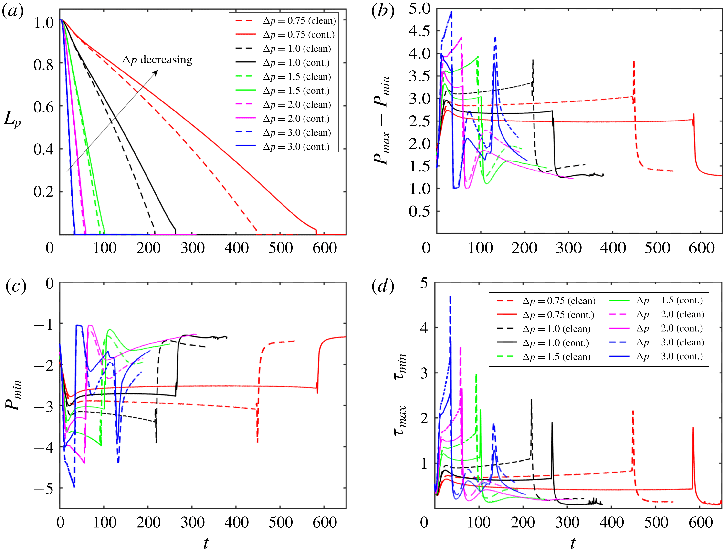The bulk surfactant concentration is $C_{0}=10^{-4}$ for the contaminated case. Figure 11 shows that both the clean and the contaminated plugs rupture earlier as $\unicode[STIX]{x0394}p$ increases. Increasing $\unicode[STIX]{x0394}p$ makes the trailing air finger move faster and thus the trailing liquid film thicker, which enhances the volume loss of the liquid plug to rupture sooner. In addition, the mechanical stresses are also intensified monotonically with increasing $\unicode[STIX]{x0394}p$ , implying an increased risk of cell injuries during the airway reopening process in deep breathing. Addition of surfactant reduces the mechanical stresses on the tube wall but it also delays plug rupture for all values of $\unicode[STIX]{x0394}p$ as expected. It is also interesting to observe that the effects of surfactant are more pronounced as $\unicode[STIX]{x0394}p$ is reduced. This can be attributed to the fact that the Marangoni stress becomes more dominant over the viscous stresses as flow velocity and thus viscous stresses decrease with decreasing $\unicode[STIX]{x0394}p$ . Plug rupture does not occur at very low values of $\unicode[STIX]{x0394}p$ . We then carry out computations to investigate the influence of the Laplace number on clean and contaminated plug rupture dynamics in the range $20\leqslant \unicode[STIX]{x1D706}\leqslant 1500$ with the other parameters held constant at their baseline values. The Laplace number is varied by changing the density of the liquid to show the effects of inertia. Figure 12 shows the effects of the Laplace number on rupture time and mechanical stresses on the airway wall. The inertial effects are clearly seen in figure 12(a) especially in the initial stage at high $\unicode[STIX]{x1D706}$ values, i.e. $\unicode[STIX]{x1D706}\geqslant 500$ . Plug rupture is delayed as $\unicode[STIX]{x1D706}$ increases and plug rupture does not occur after about $\unicode[STIX]{x1D706}\geqslant 2000$ in the present case. The effects of inertia are better reflected on the retraction of the interface after rupture as shown in figure 13. As seen, the retraction velocity $V_{snap}$ decreases significantly as $\unicode[STIX]{x1D706}$ increases mainly due to enhanced inertial effects. In general, the mechanical stresses increase as $\unicode[STIX]{x1D706}$ increases. The surfactant has effects similar to those before: it reduces the mechanical stresses and slows down airway reopening.

Figure 11.

Effects of applied pressure difference ( $\unicode[STIX]{x0394}p=p_{1}-p_{2}$ ) on plug propagation and rupture. Time evolution of (a) plug length ( $L_{p}$ ), (b) maximum difference in wall pressure ( $P_{max}-P_{min}$ ), (c) the minimum pressure on the wall and (d) maximum difference in wall shear stress ( $\unicode[STIX]{x1D70F}_{max}-\unicode[STIX]{x1D70F}_{min}$ ) for the applied pressure difference in the range $0.75\leqslant \unicode[STIX]{x0394}p\leqslant 3$ . ( $L_{pi}=1.0$ , $h_{2}=0.05$ , $\unicode[STIX]{x1D706}=100$ , $\unicode[STIX]{x1D6FD}=0.7$ , $\unicode[STIX]{x1D712}=0.01$ , $Sc=10$ , $Sc_{s}=100$ , $K_{a}=10^{4}$ , $K_{d}=100$ , $C_{0}=10^{-4}$ .)

Figure 12.

Effects of the Laplace number ( $\unicode[STIX]{x1D706}$ ) on plug propagation and rupture. Time evolution of (a) plug length ( $L_{p}$ ), (b) maximum difference in wall pressure ( $P_{max}-P_{min}$ ) and (c) maximum difference in wall shear stress ( $\unicode[STIX]{x1D70F}_{max}-\unicode[STIX]{x1D70F}_{min}$ ) for the Laplace number in the range $20\leqslant \unicode[STIX]{x1D706}\leqslant 1500$ . The solid and dashed lines show the clean and the contaminated cases, respectively. ( $L_{pi}=1.0$ , $h_{2}=0.05$ , $\unicode[STIX]{x0394}p=1$ , $\unicode[STIX]{x1D6FD}=0.7$ , $\unicode[STIX]{x1D712}=0.01$ , $Sc=10$ , $Sc_{s}=100$ , $K_{a}=10^{4}$ , $K_{d}=100$ , $C_{0}=10^{-4}$ .)

Figure 13.

Effects of the Laplace number ( $\unicode[STIX]{x1D706}$ ) on the retraction of the interface after plug rupture for the Laplace number in the range $20\leqslant \unicode[STIX]{x1D706}\leqslant 1500$ . The solid and dashed lines show the clean and the contaminated cases, respectively. ( $L_{pi}=1.0$ , $h_{2}=0.05$ , $\unicode[STIX]{x0394}p=1$ , $\unicode[STIX]{x1D6FD}=0.7$ , $\unicode[STIX]{x1D712}=0.01$ , $Sc=10$ , $Sc_{s}=100$ , $K_{a}=10^{4}$ , $K_{d}=100$ , $C_{0}=10^{-4}$ .)

Figure 14.

Effects of the non-dimensional adsorption and desorption coefficients on plug propagation and rupture. Time evolution of (a) plug length ( $L_{p}$ ), (b) maximum difference in wall pressure ( $P_{max}-P_{min}$ ) and (c) maximum difference in wall shear stress ( $\unicode[STIX]{x1D70F}_{max}-\unicode[STIX]{x1D70F}_{min}$ ). ( $L_{pi}=1.0$ , $h_{2}=0.05$ , $C_{0}=10^{-4}$ , $\unicode[STIX]{x0394}p=1$ , $\unicode[STIX]{x1D706}=100$ , $\unicode[STIX]{x1D6FD}=0.7$ , $\unicode[STIX]{x1D712}=0.01$ , $Sc=10$ , $Sc_{s}=100$ .)

Further simulations are performed to examine the effects of the non-dimensional adsorption and desorption coefficients ( $K_{a}$ and $K_{d}$ ), Schmidt numbers ( $Sc$ and $Sc_{s}$ ) and the dimensionless adsorption depth ( $\unicode[STIX]{x1D712}$ ). The non-dimensional adsorption and desorption coefficients are varied together such that their ratio is constant at $K_{a}/K_{d}=100$ and the other parameters are fixed at their baseline values. Note that the vanishing values of $K_{a}$ and $K_{b}$ correspond to the insoluble case that will be discussed later separately. Simulations are performed for values of $(K_{a},K_{d})=(10^{3},10)$ , $(10^{4},10^{2})$ and $(10^{5},10^{3})$ , and the results are shown in figures 14 and 15. As seen in figure 15, the surfactant concentration is reduced significantly at the interface of the leading meniscus as $K_{a}$ and $K_{d}$ are increased since the concentration exceeds the equilibrium value (e.g. $\unicode[STIX]{x1D6E4}_{eq}\approx 0.01$ ) there and is released back into the bulk liquid more quickly at higher values of $K_{a}$ and $K_{d}$ . As a result, the overall effect of the surfactant is decreased as $K_{a}$ and $K_{d}$ are increased (figure 14). We then investigate the effects of molecular diffusivity. Enhanced molecular diffusivity smooths the interfacial surfactant distribution more effectively and thus reduces the Marangoni stresses. It is therefore expected that the effect of surfactant increases as the Schmidt number increases, which is confirmed in figure 16 where the simulation results are shown for Schmidt numbers in the range $1\leqslant Sc\leqslant 100$ and $10\leqslant Sc_{s}\leqslant 1000$ together with the results obtained for the clean case. This figure shows that the plug rupture is delayed and the mechanical stresses are reduced as the Schmidt number is increased. The adsorption depth characterizes the depth beneath the interface diluted by surfactant adsorption and it decreases as the bulk surfactant concentration $C_{0}$ increases. Therefore increasing $\unicode[STIX]{x1D712}$ is expected to have a qualitatively similar effect to decreasing $C_{0}$ . Figure 17 shows the effects of the adsorption depth on the plug rupture and the maximum difference in wall pressure in the range $0.001\leqslant \unicode[STIX]{x1D712}\leqslant 1$ . As seen, plug rupture is slightly delayed and the maximum difference in wall pressure is slightly decreased with increasing $\unicode[STIX]{x1D712}$ . Although not shown here, the shear stress is also reduced slightly as $\unicode[STIX]{x1D712}$ is increased.

Figure 15.

Effects of the non-dimensional adsorption and desorption coefficients on interfacial surfactant concentration and surface velocity distributions at $t=t_{rupture}$ . ( $L_{pi}=1.0$ , $h_{2}=0.05$ , $C_{0}=10^{-4}$ , $\unicode[STIX]{x0394}p=1$ , $\unicode[STIX]{x1D706}=100$ , $\unicode[STIX]{x1D6FD}=0.7$ , $\unicode[STIX]{x1D712}=0.01$ , $Sc=10$ , $Sc_{s}=100$ .)

Figure 16.

Effects of the Schmidt numbers on plug propagation and rupture. Time evolution of (a) plug length ( $L_{p}$ ), (b) maximum difference in wall pressure ( $P_{max}-P_{min}$ ) and (c) maximum difference in wall shear stress ( $\unicode[STIX]{x1D70F}_{max}-\unicode[STIX]{x1D70F}_{min}$ ). ( $L_{pi}=1.0$ , $h_{2}=0.05$ , $C_{0}=10^{-4}$ , $\unicode[STIX]{x0394}p=1$ , $\unicode[STIX]{x1D706}=100$ , $\unicode[STIX]{x1D6FD}=0.7$ , $\unicode[STIX]{x1D712}=0.01$ , $K_{a}=10^{4}$ , $K_{d}=100$ .)

Figure 17.

Time evolution of the plug length ( $L_{p}$ ) for various values of dimensionless adsorption depth ( $\unicode[STIX]{x1D712}$ ). The inset shows time evolution of maximum difference in wall pressure ( $P_{max}-P_{min}$ ). ( $L_{pi}=1.0$ , $h_{2}=0.05$ , $C_{0}=10^{-4}$ , $\unicode[STIX]{x0394}p=1$ , $\unicode[STIX]{x1D706}=100$ , $\unicode[STIX]{x1D6FD}=0.7$ , $Sc=10$ , $Sc_{s}=100$ , $K_{a}=10^{4}$ , $K_{d}=100$ .)

Figure 18.

Effects of surfactant solubility. Time evolution of (a) plug length ( $L_{p}$ ), (b) maximum difference in wall pressure ( $P_{max}-P_{min}$ ) and (c) maximum difference in wall shear stress ( $\unicode[STIX]{x1D70F}_{max}-\unicode[STIX]{x1D70F}_{min}$ ). (d) The interface surfactant concentration and Marangoni stress distributions at $t-t_{rupture}=0.52$ for $C_{0}\leqslant 5\times 10^{-4}$ , and at $t=452.84$ and $t=605.89$ for $C_{0}=5\times 10^{-4}$ for the soluble and insoluble cases, respectively. For the insoluble cases, $C_{0}$ is used to determine the initial equilibrium concentration at the interface. ( $L_{pi}=1.0$ , $h_{2}=0.05$ , $\unicode[STIX]{x0394}p=1$ , $\unicode[STIX]{x1D6FD}=0.7$ , $\unicode[STIX]{x1D712}=0.01$ , $Sc=10$ , $Sc_{s}=100$ , $K_{a}=10^{4}$ , $K_{d}=100$ , $C_{0}=10^{-4}$ .)

In many theoretical and numerical studies, surfactant solubility is ignored to simplify the analysis. We finally examine the effects of surfactant solubility on plug rupture dynamics. For this purpose, the adsorption and desorption coefficients are set to zero, i.e. $k_{a}^{\ast }=k_{d}^{\ast }=0$ , and computations are carried out for the bulk surfactant concentration in the range $10^{-5}\leqslant C_{0}\leqslant 5\times 10^{-4}$ . The results are shown in figure 18 where the fully soluble simulation results obtained using the baseline parameters are also plotted to facilitate a direct comparison. As seen, the surfactant solubility becomes more pronounced as the bulk surfactant concentration increases. Since the overall effect of surfactant is small at a very small bulk concentration (e.g. at $C_{0}=10^{-5}$ ) as seen in figure 5, it is safe to say that the surfactant solubility is generally important and should be taken into account in a plug rupture analysis.