2. Preliminaries

The preliminaries are largely the same as for [Reference Janson10] so we will try to keep this short, and refer readers to [Reference Janson10] for a more detailed description. For our fixed, finite alphabet $\mathcal A$ we define $\mathcal A^\ast \,:\!=\, \bigcup_{n=0}^\infty\mathcal A^n$ as the set of finite strings over $\mathcal A$ . The elements of strings are called characters. We write $\varepsilon$ for the empty string and $\alpha\beta$ for the concatenation of strings $\alpha,\beta \in \mathcal A^\ast$ . We extend this notation to sets of strings in the usual manner, with $aT \,:\!=\, \{at \mid t\in T\}$ for $T\subseteq \mathcal A^\ast,a\in \mathcal A^\ast$ . As noted before, we have a probability measure p on $\mathcal A$ , with point masses $p_a \in (0,1), a\in \mathcal A$ . For a string $\alpha = (a_1, a_2, \dots, a_n) \in \mathcal A^\ast$ , we define by extension $p_\alpha \,:\!=\, p_{a_1}\dots p_{a_n}$ .

This set $\mathcal A^\ast$ can naturally be identified with the nodes of the infinite $| \mathcal A |$ -ary tree, with a node $a\in \mathcal A^\ast$ being an ancestor of a node $b\in \mathcal A^\ast$ if and only if a is a prefix of b. We call subtrees of $\mathcal A^\ast$ including the root $\mathcal A$ -ary trees and associate them with their node set $T\subset \mathcal A^\ast$ . For technical reasons, we also consider the empty graph $\emptyset$ as a tree. Associating the trees with their node sets forms a bijection between $\mathcal A$ -ary trees and subsets $T\subset \mathcal A^\ast$ with the property that for all $a\in T$ all prefixes of a are also in T. We write $\mathfrak T$ for the set of $\mathcal A$ -ary trees and let $\bullet \,:\!=\, \{\varepsilon\}$ be the tree consisting only of the root.

For a set $T\subset \mathcal A^\ast \cup \mathcal A^{\mathbb{N}}$ of finite or infinite strings and a finite string $v\in \mathcal A^\ast$ , we define $T^v$ as the strings starting with v with v removed. In exact terms, that means $T^v \,:\!=\, \{\alpha\mid v\alpha\in T\}$ . If T is a tree and v a node of T, we call $T^v$ the fringe tree. It is then the subtree of T consisting of v and its descendants.

Given a finite set $\mathfrak X \subseteq \mathcal A^\ast \cup \mathcal A^{\mathbb{N}}$ of (finite or infinite) strings where no string is a prefix of another, the trie $T(\mathfrak X)$ is a $\mathcal A$ -ary tree defined as follows; see [Reference Jacquet and Szpankowski7, Section 6.1] and [Reference Knuth11, Chapter 6.3]. The trie for the empty set is empty. The trie for a single string consists of only one leaf, the root. We say that this leaf stores the string. The interesting case is the last: the trie for multiple strings consists of the root, and for every character $a\in \mathcal A$ this root has a child with the subtree being a trie built from $\mathfrak X^a$ , the strings starting with a. We are therefore splitting the set of strings into subtrees by their first character. Formally, we have $T(\emptyset) \,:\!=\, \emptyset$ , for $| \mathfrak X | = 1$ we have $T(\mathfrak X) \,:\!=\, \bullet$ , and for $| \mathfrak X | \ge 2$

(1) \begin{equation}T(\mathfrak X) \,:\!=\,\{\varepsilon\} \cup \displaystyle\bigcup_{a\in\mathcal A} aT(\mathfrak X^a).\end{equation}

In the patricia trie, introduced by Morrison [Reference Morrison12] in 1968, a node v can additionally store a string $I_v$ as the common prefix of all strings that are stored in leaves under it. We write $\operatorname{lcp}(T)$ for the longest common prefix of a set $T\subset \mathcal A^\ast \cup \mathcal A^{\mathbb{N}}$ of strings. The patricia trie for one or zero strings is the same as the trie. For multiple strings, the longest common prefix $\operatorname{lcp}(\mathfrak X)$ is saved in an attribute I of the root, and the splitting is done on the first character that not all strings have in common. Thus, for every character $a\in A$ , the root has as subtree the patricia trie built from $\mathfrak X^{\operatorname{lcp}(\mathfrak X)a}$ , the strings starting with $\operatorname{lcp}(\mathfrak X)a$ . Formally, we define $\operatorname{pat} T(\emptyset)$ as $\emptyset$ and $\operatorname{pat} T(\mathfrak X) = \bullet$ for $| \mathfrak X | = 1$ as for tries. For $| \mathfrak X | \ge 2$ we define

\begin{equation*}\operatorname{pat} T(\mathfrak X) \,:\!=\,\{\varepsilon\} \cup \displaystyle\bigcup_{a\in\mathcal A}a \operatorname{pat} T(\mathfrak X^{\operatorname{lcp}(\mathfrak X)a}).\end{equation*}

Then the common prefix $\operatorname{lcp}(\mathfrak X)$ is stored in the attribute $I_\varepsilon$ of the root, and for every $a\in\mathcal A$ , $\alpha\in\mathcal A^\ast$ the attribute $I_{a\alpha}$ will be the attribute $I_{\alpha}$ of 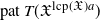$\operatorname{pat} T(\mathfrak X^{\operatorname{lcp}(\mathfrak X)a})$ . While the patricia trie technically consists of the tree and the map $v \mapsto I_v$ of the common prefixes, we usually regard it as a tree and ignore the additional structure when convenient.

We use $\operatorname{pat} T(\mathfrak X)$ as suggestive notation to emphasize the fact that the patricia trie can also be constructed from the trie. For a trie T, the patricia trie $\operatorname{pat}(T)$ for the same strings is constructed by iteratively merging every node $\nu\in\mathcal A^\ast$ with exactly one child $\nu a$ for $a\in \mathcal A$ with its child and prepending the character a to the attribute $I_\nu$ of the merged node. Conversely, by adding a parent with only one child for every character in $I_\nu$ , for every node $\nu$ one can construct the trie from the patricia trie. With simple induction one can show that the two definitions are actually equivalent, so that we have $\operatorname{pat}(T(\mathfrak X)) = \operatorname{pat} T(\mathfrak X)$ .

Let $\mathcal{T}_n$ denote the random trie generated by $n\in \mathbb{N}$ i.i.d. infinite strings, where each character is i.i.d. sampled from the distribution p and $\mathcal{P}_n = \operatorname{pat}(\mathcal{T}_n)$ is the patricia trie from the same strings. We also consider a Poisson version, where we construct the trie from a $\operatorname{Poi}(\lambda)$ -distributed number $N_\lambda$ of strings for $\lambda \ge 0$ , with $N_\lambda$ independent of the strings. We define $\widetilde{\mathcal{T}}_{:\lambda}= \mathcal{T}_{N_\lambda}$ and $\widetilde{\mathcal{P}}_\lambda \,:\!=\, {\mathcal{P}}_{N_\lambda} = \operatorname{pat}(\widetilde{\mathcal{T}}_{\lambda})$ .

The properties that we study are represented as so-called additive functionals. Given a function $\varphi\colon \mathfrak T \to \mathbb{R}^n, n\ge1$ with $\varphi(\varnothing) =0$ , we define the corresponding additive functional $\Phi\colon \mathfrak T \to \mathbb{R}^n$ as

(2) \begin{equation}\Phi(T) = \sum_{\alpha\in \mathcal A^\ast} \varphi(T^\alpha)= \sum_{v\in T} \varphi(T^v).\end{equation}

This can be written recursively as

\begin{equation*}\Phi(T) = \varphi(T) + \sum_{a\in\mathcal A}\Phi(T^a),\quad \Phi(\varnothing)=0,\end{equation*}

which also shows that every function $\Phi\colon \mathfrak T \to \mathbb{R}^n$ with $\Phi(\varnothing)=0$ can be represented as an additive functional. The term ‘additive functional’ for $\Phi$ is thus mainly defined by its relation to $\varphi$ , which is called the toll function of $\Phi$ . For example, if we define

\begin{equation*}\varphi_i(T) \,:\!=\, \mathbf{1}\{{\textit{T} \, \, \mathrm{has \, \, more \, \, than \, \, 1 \, \, node}}\},\end{equation*}

then the corresponding additive functional $\Phi_i$ counts the internal nodes of a tree. For a patricia trie $\operatorname{pat} T(\mathfrak X)$ , we assume that $\Phi(\operatorname{pat} T(\mathfrak X))$ only depends on the patricia trie regarded as an $\mathcal A$ -tree and ignores the additional attributes $I_v$ .

We use the notation $\overset d\longrightarrow$ for convergence in distribution and $\overset d\approx$ for approximation in distribution, i.e. for two sequences $X_n$ and $Y_n$ of random variables on the same Borel space S, $X_n \overset d\approx Y_n$ holds if and only if, for all bounded, continuous functions $f\colon S\to \mathbb{R}$ ,

(3) \begin{equation}|\mathbb{E}[f(X_n)] - \mathbb{E}[f(Y_n)]| \longrightarrow 0 \quad \mathrm{as}\ n\to\infty.\end{equation}

If $S=\mathbb{R}$ , we say that this approximation holds with all moments if (3) is also true for $f(x)=| x |^r$ , $r>0$ and $f(x) = x^s$ , $s\in\mathbb{N}$ . Compare Appendix B of [Reference Janson10]. Furthermore, we write H for the entropy of the source p, that is,

\begin{equation*}H \,:\!=\, \sum_{a\in\mathcal A} p_a\log\biggl({\dfrac1{p_a}}\biggr).\end{equation*}

For complex $s\in \mathbb{C}$ , let

(4) \begin{equation}\rho(s) \,:\!=\, \sum_{a\in\mathcal A}p_a^s.\end{equation}

For natural $s\in \mathbb{N}$ , we may interpret this as the probability for s strings to start with the same character.

3. Patricia trie and trie

We now relate additive functionals on patricia tries to those on tries.

Proposition 1. An additive functional $\Phi$ on patricia tries defines an additive functional $\widehat{\Phi} \,:\!=\, \Phi\circ \operatorname{pat} $ on tries by pullback with $\operatorname{pat}$ . The toll function $\widehat{\varphi}(T)$ of $\widehat{\Phi}$ is given by

\begin{equation*}\widehat{\varphi}(T) = \begin{cases}0 & T\mbox{'}\!s\ root\ has\ exactly\ one\ child, \\ \varphi(\operatorname{pat}(T)) & {else.}\end{cases}\end{equation*}

Since then $\Phi(\mathcal{P}_n) = \widehat{\Phi}(\mathcal{T}_n)$ , all results about additive functionals on tries can be extended to patricia tries by just exchanging the toll function $\varphi$ with $\widehat{\varphi}$ if the conditions are still satisfied. There is an alternative way to write $\widehat{\varphi}$ : by defining

(5) \begin{equation}\varphi_p(T) \,:\!=\, \mathbf{1} \{{\textit{T}} \, \text{does not have exactly one child} \},\end{equation}

we have $\widehat{\varphi}(T) = \varphi_p(T)\varphi({\operatorname{pat}(T)})$ for all toll functions $\varphi$ .

4. Limit theorems

We reformulate the main Theorem 3.9 of [Reference Janson10] for patricia tries. Let $\Phi$ be an additive functional on patricia tries. We call the functional increasing if, for every two sets $\mathfrak X \subseteq \mathfrak Y \subset \mathcal A^{\mathbb{N}}$ of strings, we have $\Phi({\operatorname{pat}(T(\mathfrak X))}) \le \Phi({\operatorname{pat}(T(\mathfrak Y))})$ . In other words, $\Phi$ is increasing if and only if $\Phi\circ\operatorname{pat}\circ T = \widehat{\Phi} \circ T$ is monotone. Note that this is not the same as $\Phi$ being increasing as an additive functional on tries as in [Reference Janson10]: in patricia tries, new leaves can also grow out of edges, making functionals such as ‘number of edges that connect two nodes with more than three children’ not increasing.

Let $\Phi$ be an additive functional on patricia tries and let $\widehat{\Phi}$ be the corresponding pullback on tries as defined in Proposition 1, with toll function $\widehat{\varphi}$ . Let $\chi \,:\!=\, \varphi(\bullet)$ be the value every leaf contributes to $\Phi$ . The leaves have to be treated as a special case in the analysis of patricia tries (and tries) because their behavior is substantially different from internal nodes. However, their number is simply n in $\mathcal{P}_n$ and $N_\lambda$ in $\widetilde{\mathcal{P}}_\lambda$ , and we use $\chi$ only to accommodate for this fact.

To express the asymptotics for mean and variance, we need the following functions, where the terms are much simpler for $\chi=0$ :

(6) \begin{align} f_E(\lambda) & \,:\!=\, \mathbb{E}\bigl[{\widehat{\varphi}(\widetilde{\mathcal{T}}_{\lambda})}\bigr]- \chi \lambda {\mathrm{e}}^{-\lambda} ,\\[-10pt]\nonumber\end{align}

(7) \begin{align} f_V(\lambda) & \,:\!=\, 2\operatorname{Cov}\bigl({\widehat{\varphi}(\widetilde{\mathcal{T}}_{\lambda}), \widehat{\Phi}(\widetilde{\mathcal{T}}_{\lambda})}\bigr)- \operatorname{Var}\bigl({\widehat{\varphi}(\widetilde{\mathcal{T}}_{\lambda})}\bigr)\nonumber\\&\quad\,+ 2\chi \lambda {\mathrm{e}}^{-\lambda}\bigl(\mathbb{E}\widehat{\Phi}(\widetilde{\mathcal{T}}_{\lambda})-\mathbb{E}\widehat{\varphi}(\widetilde{\mathcal{T}}_{\lambda})\bigr)- \chi^2\lambda {\mathrm{e}}^{-\lambda}(1-\lambda {\mathrm{e}}^{-\lambda}),\\[-10pt]\nonumber\end{align}

(8) \begin{align}f_C(\lambda) & \,:\!=\, \operatorname{Cov}\bigl({\widehat{\varphi}(\widetilde{\mathcal{T}}_{\lambda}), N_\lambda}\bigr) + \chi \lambda(\lambda-1)\,{\mathrm{e}}^{-\lambda}.\end{align}

In the convenient case of $\chi=0$ , this simplifies to

(9) \begin{align} f_E(\lambda) &= \mathbb{E}{\bigl[\widehat{\varphi}(\widetilde{\mathcal{T}}_{\lambda})\bigr]},\\[-13pt]\nonumber\end{align}

(10) \begin{align} f_V(\lambda) &= 2\operatorname{Cov}\bigl({\widehat{\varphi}(\widetilde{\mathcal{T}}_{\lambda}), \widehat{\Phi}(\widetilde{\mathcal{T}}_{\lambda})}\bigr)- \operatorname{Var}\bigl({\widehat{\varphi}(\widetilde{\mathcal{T}}_{\lambda})}\bigr),\\[-13pt]\nonumber\end{align}

(11) \begin{align} f_C(\lambda) &= \operatorname{Cov}\bigl({\widehat{\varphi}(\widetilde{\mathcal{T}}_{\lambda}), N_\lambda}\bigr). \end{align}

Now for $X=E,V,C$ we define the Mellin transform of $f_X$ as

(12) \begin{equation}f_X^\ast(s) \,:\!= \int_0^\infty t^{s-1}f_X(t)\,{\mathrm{d}} t,\end{equation}

for $s\in \mathbb{C}$ where the integral converges absolutely.

For certain distributions p, there are typically oscillations in mean and variance of additive functionals. These occur if there is a number $d_p$ such that

(13) \begin{equation}\{\log p_a \mid a \in \mathcal A\} \subseteq d_p\mathbb{Z}.\end{equation}

We then define $d_p$ to be the biggest such number. If there is no such number, we define $d_p \,:\!=\, 0$ . An alternative characterization is to define $d_p$ as the infimum of positive elements of the additive subgroup generated by $\{\log p_a \mid a \in \mathcal A\}$ .

If $d_p=0$ , there are no oscillations, and we define

(14) \begin{equation}\psi_X(t) \,:\!=\, f_X^\ast({-}1)\end{equation}

as constant functions. If $d_p > 0$ , we define $\psi_X$ as bounded, continuous, $d_p$ -periodic functions with the Fourier series

(15) \begin{equation}\psi_X(t) \sim \sum_{m=-\infty}^\infty f_X^\ast\biggl({-1-\dfrac{2\pi m}{d_p}{\mathrm{i}}}\biggr)\,{\mathrm{e}}^{{2\pi {\mathrm{i}} mt}/{d_p}}.\end{equation}

Moreover, if $X=E$ or if $f'_X(\lambda) = {\mathrm{O}}(\lambda^{-\varepsilon_1})$ as $\lambda\to\infty$ for some $\varepsilon_1>0$ , Theorem 3.1 of [Reference Janson10] shows that the Fourier series (15) converges absolutely, and thus ‘ $\sim$ ’ may be replaced by ‘ $=$ ’ in (15). Lemma 3.6 of [Reference Janson10] further shows that $\psi_C(t) = \psi_E(t) + \psi_E'(t)$ for all values of t, so that we actually just need to compute $\psi_E$ and $\psi_V$ . Typically, the values

\[f_X^\ast\biggl({-1-\frac{2\pi m}{d_p}{\mathrm{i}}}\biggr)\]

are small for $m \ne 0$ , so we can still consider the mean term $f_X^\ast({-}1)$ as ‘average asymptotic value’.

With these values and definitions, we can finally state our version of Theorem 3.9 of [Reference Janson10].

Remark 1. The assumption of boundedness on $\phi_+, \phi_-$ can, as in [Reference Janson10], be weakened to show that for some $\varepsilon > 0$ ,

\begin{equation*}\mathbb{E}{\bigl[\phi_\pm(\widetilde{\mathcal{T}}_{\lambda})\bigr]} ={\mathrm{O}}(\lambda^{1-\varepsilon}),\quad \text{Var}(\phi_\pm(\widetilde{\mathcal{T}}_{\lambda})) = {\mathrm{O}}(\lambda^{1- \varepsilon}),\end{equation*}

and that there exists some $r > 2$ such that

\begin{equation*}\mathbb{E}\bigl| {\phi_\pm(\widetilde{\mathcal{T}}_{\lambda}) - \mathbb{E}\phi_\pm(\widetilde{\mathcal{T}}_{\lambda})}\bigr|^r = {\mathrm{O}}(\lambda^{r/2}).\end{equation*}

The convergence (18) then only holds for moments $s < r$ ; see Theorem 5.8 of [Reference Janson10].

From his version of Theorem 1, Janson derives a weak law of large numbers, while leaving as an open question if one also had almost sure (a.s.) convergence. Using a proof technique for the strong law of large numbers for sums of i.i.d. random variables with a finite fourth absolute moment, we can show a.s. convergence. We have the following strong law of large numbers for patricia tries. The same proof can be applied to tries, answering the open question.

Theorem 2. Let $\varphi$ be a bounded toll function on patricia tries as in Theorem 1. Then, as $n\to\infty$ ,

(20) \begin{equation}\dfrac{\Phi(\mathcal{P}_n)}{n} - H^{-1} \psi_E(\kern-2.2pt\log(n)) - \chi\longrightarrow 0\quad\textit{a.s.}\end{equation}

In particular, if $d_p=0$ , then, as $n\to\infty$ ,

\begin{equation*} \dfrac{\Phi(\mathcal{P}_n)}n \longrightarrow H^{-1} f_E^\ast({-}1) + \chi \quad\textit{a.s.}\end{equation*}

Proof. Note that $\mathbb{E}[\Phi(\mathcal{P}_n)]$ is asymptotically $H^{-1} \psi_E(\kern-2.2pt\log \lambda) + \chi$ according to (19). So (20) is equivalent to showing that $n^{-1} Z_n \,:\!=\, n^{-1}(\Phi(\mathcal{P}_n) - \mathbb{E}\Phi(\mathcal{P}_n)) \to 0$ a.s. Writing out the quantifiers of ‘not converging’, we have

(21) \begin{equation}\biggl\{{\dfrac{Z_n}n \not\to 0}\biggr\} = \bigcup_{m\in\mathbb{N}}\bigcap_{N=1}^\infty\bigcup_{n=N}^\infty \biggl\{{\biggl|{\dfrac{Z_n}n}\biggr|>\dfrac1m}\biggr\}= \bigcup_{m\in\mathbb{N}} \limsup_{n\to \infty}\biggl\{{\biggl| {\dfrac{Z_n}n}\biggr|>\dfrac1m}\biggr\}.\end{equation}

Since we have convergence of all moments of $Z_n/\sqrt n$ in (16), we have $\mathbb{E}| Z_n/n |^4 \le C/n^2$ for a constant $C>0$ and all $n\ge1$ . Markov’s inequality implies

\begin{equation*} \sum_{n=1}^\infty \mathbb{P}{\biggl(\biggl| {\dfrac{Z_n}n}\biggr|>\dfrac1m\biggr)}= \sum_{n=1}^\infty \mathbb{P}{\biggl(\biggl| {\dfrac{Z_n}n}\biggr|^4>\dfrac1{m^4}\biggr)}\le \sum_{n=1}^\infty \dfrac{m^4C}{n^2} < \infty,\end{equation*}

hence the Borel–Cantelli lemma yields

\[\mathbb{P}{\biggl(\limsup_{n\to \infty}\biggl\{{\biggl| {\dfrac{Z_n}n}\biggr|>\dfrac1m}\biggr\}\biggr)}=0\]

for all $m\ge1$ . In view of (21), subadditivity implies the assertion.

5. Applications

With Theorem 1, we can calculate the asymptotic distribution of random fringe trees in patricia tries. Furthermore, we show another application, the independence number, to demonstrate how to use this theorem without a closed formula for the functions $f_E, f_V$ .

5.1. Fringe patricia tries

Our main application is the study of random fringe trees $\mathcal{P}_n^\ast$ of patricia tries. We want to first study the size $| \mathcal{P}_n^\ast |_e$ , as measured in number of leaves or equivalently strings. We count the number of subtrees of size $k\ge1$ with the functional

\begin{equation*}\varphi_k(T) \,:\!=\, \mathbf{1}\{|T|_e=k\}.\end{equation*}

Note that subtrees of size 1 are the leaves, so $\varphi_1 = \varphi_\bullet = \widehat{\varphi}_\bullet$ . This case behaves differently from the others and is trivial, so we will first consider only $k\ge2$ .

While $\Phi_k$ is not increasing, it can be written as $\Phi_{\geq k}-\Phi_{\geq k+1}$ , where $\varphi_{\geq k} \,:\!=\, \mathbf{1}\{|T|_e\geq k\}$ is bounded and $\Phi_{\geq k}$ is increasing, so we can apply Theorems 1 and 2.

We present two ways to get results about fringe patricia tries. One way is to directly calculate $f_{E,k}, f_{E,k}^\ast$ etc. Another way is to directly link fringe trees on tries with those on patricia tries. For those, we first have to understand what differs from tries: the common prefixes.

Lemma 1. Let T be a fixed $\mathcal A$ -nary tree where no node has outdegree 1 and $k \,:\!=\, |T|_e$ . Let $T_e \subset \mathcal A^\ast$ be its leaves and let $T_i$ be its internal nodes. The probability $p_T \,:\!=\, \mathbb{P}(\mathcal{P}_k = T)$ of a random patricia trie of size k being T is given by

\begin{equation*}p_T = k!\prod_{v \in T_e} p_v \prod_{w\in T_i} \dfrac1{1-\rho(|T^w|_e)}.\end{equation*}

Conditioned on the tree structure of $\mathcal{P}_k$ being given by T, the common prefixes per node are independent. In an internal node $v\in T_i$ , their distribution is given by $q_{|T^v|_e}$ , with $q_i$ , $i\ge2$ defined as

\begin{equation*}q_i(\{\alpha\}) \,:\!=\, p_\alpha^i (1-\rho(i));\;\alpha\in\mathcal A^\ast.\end{equation*}

Thus the length $| I |_v$ is $\operatorname{Geom}_0({1-\rho({| T^v |_e})})$ -distributed, where we use $\operatorname{Geom}_0$ to refer to the geometric distribution with support $\mathbb{N}_0$ and $\operatorname{Geom}_1$ to the one with support $\mathbb{N}^+$ .

We will prove Lemma 1 at the end of this section. The trie can be reconstructed from the tree structure and the common prefixes of the patricia trie. As $\operatorname{pat}$ is compressing chains of nodes into the common prefixes, the inverted process basically expands those common prefixes into a chain of nodes. Every fringe patricia trie $T^v$ of size k then corresponds to $| I_v | + 1$ fringe tries of size k. By Lemma 1, $\Phi_k(\mathcal{T}_n)$ is thus distributed as the sum of $\Phi_k(\mathcal{P}_n)$ $\operatorname{Geom}_1(1-\rho(k))$ -distributed, independent random variables. This immediately links mean and variance of the number of fringe trees of size k:

\begin{align*}\mathbb{E}[{\Phi_k(\mathcal{T}_n)}] &= \dfrac1{1-\rho(k)}\mathbb{E}{[\Phi_k(\mathcal{P}_n)]}{,}\\\operatorname{Var}({\Phi_k(\mathcal{T}_n)}) &= \mathbb{E} [{\operatorname{Var}(\Phi_k(\mathcal{T}_n) \mid \Phi_k(\mathcal{P}_n))}]+ \operatorname{Var}({\mathbb{E}{[\Phi_k(\mathcal{T}_n) \mid \Phi_k(\mathcal{P}_n)]}})\nonumber\\&= \dfrac{\rho(k)}{(1-\rho(k))^2} \mathbb{E}{[\Phi_k(\mathcal{P}_n)]}+ \dfrac1{(1-\rho(k))^2}\operatorname{Var}(\Phi_k(\mathcal{P}_n)).\end{align*}

For fixed k, mean and variance for patricia tries are hence just linear combinations of mean and variance for tries, so this will also hold for $f_{E,k}, f_{V,k}$ and their Mellin transforms $f_{E,k}^\ast, f_{V,k}^\ast$ .

Nevertheless, we show how to calculate them directly, starting with the mean. From Proposition 1 and (5) we have $\widehat{\varphi}_k(\widetilde{\mathcal{T}}_{\lambda}) = \mathbf{1}\{N_\lambda = k\}\varphi_p(\widetilde{\mathcal{T}}_{\lambda})$ , so the mean function is given by

(22) \begin{align}f_{E,k}(\lambda) &= \mathbb{E}\bigl[{\widehat{\varphi}_k(\widetilde{\mathcal{T}}_{\lambda})}\bigr]\notag \\&= \mathbb{P}(N_\lambda = k)\mathbb{E}\bigl[\varphi_p(\widetilde{\mathcal{T}}_{\lambda})\mid N_\lambda=k\bigr]\nonumber\\&= \dfrac{\lambda^k}{k!}\,{\mathrm{e}}^{-\lambda}\Biggl({1-\sum_{a\in\mathcal A}p_a^k}\Biggr)\notag \\&= \dfrac{\lambda^k}{k!}\,{\mathrm{e}}^{-\lambda}({1-\rho(k)})\end{align}

with $\rho(k)$ as defined in (4). By the definition of the Gamma function $\Gamma$ , the Mellin transform is given by

(23) \begin{align}f^\ast_{E,k}(s) = (1-\rho(k))\dfrac{\Gamma(k+s)}{k!},\quad f^\ast_{E,k}({-}1) = \dfrac{1-\rho(k)}{k(k-1)}.\end{align}

Now to the variance. The function $f_{V,k}$ is given by

\begin{equation*}f_{V,k}(\lambda) \,:\!=\, 2\operatorname{Cov}\bigl({\widehat{\varphi}_k(\widetilde{\mathcal{T}}_{\lambda}), \widehat{\Phi}_k(\widetilde{\mathcal{T}}_{\lambda})}\bigr)- \operatorname{Var}\bigl({\widehat{\varphi}(\widetilde{\mathcal{T}}_{\lambda})}\bigr).\end{equation*}

Note that if $\widehat{\varphi}_k(\widetilde{\mathcal{T}}_{\lambda})$ is 1, that is, if the root has more than one child and there are k strings in the trie, all other nodes must have less than k strings. So then $\widehat{\Phi}_k(\widetilde{\mathcal{T}}_{\lambda}) = 1$ . We then use monotone convergence to show

(24) \begin{align}f_{V,k}(\lambda) &= \mathbb{E}{\bigl[\widehat{\varphi}_k(\widetilde{\mathcal{T}}_{\lambda})\bigr]} - 2\mathbb{E}{\bigl[\widehat{\varphi}_k(\widetilde{\mathcal{T}}_{\lambda})\bigr]}\mathbb{E}{\bigl[\widehat{\Phi}_k(\widetilde{\mathcal{T}}_{\lambda})\bigr]} + \mathbb{E}{\bigl[\widehat{\varphi}_k(\widetilde{\mathcal{T}}_{\lambda})\bigr]}^2\nonumber\\&= f_{E,k}(\lambda) - 2\sum_{\alpha\in \mathcal A^\ast}f_{E,k}(\lambda)\mathbb{E}{\bigl[\widehat{\varphi}_k(\widetilde{\mathcal{T}}_{^\lambda}\alpha)\bigr]} + f_{E,k}^2(\lambda) \nonumber\\&= f_{E,k}(\lambda) - 2\sum_{\alpha\in \mathcal A^\ast} f_{E,k}(\lambda)f_{E,k}(p_\alpha \lambda) + f_{E,k}^2(\lambda).\end{align}

The last equality is because $\widetilde{\mathcal{T}}_{^\lambda}\alpha$ is the trie of the strings starting with $\alpha$ (at least if it exists), a fact which can be directly deduced from the definition in (1). Since the number of strings starting with $\alpha$ is $\operatorname{Poi}(\lambda p_\alpha)$ -distributed, $\widehat{\varphi}_k(\widetilde{\mathcal{T}}_{^\lambda}\alpha)$ is distributed as $\widehat{\varphi}_k(\widetilde{\mathcal{T}}_{[\lambda}p_\alpha])$ . Note that the last term is the term in the sum for $\alpha = \varepsilon$ . Sums like in (24) show up often in the analysis of $f_V$ , so Janson defines the shorthand ${\sum_\alpha}^\ast \,:\!=\, \sum_{\alpha\in\mathcal A^\ast} + \sum_{\alpha\in\mathcal A^\ast\backslash\{\varepsilon\}}$ , which summarizes our last two terms. We can then substitute $f_{E,k}$ using (22):

\begin{equation*}f_{V,k}(\lambda) = \dfrac{1-\rho(k)}{k!}\lambda^k {\mathrm{e}}^{-\lambda} - {\sum_\alpha}^\ast{\biggl(\dfrac{1-\rho(k)}{k!}\biggr)}^2 \lambda^{2k}p_\alpha^k {\mathrm{e}}^{-\lambda(1+p_\alpha)}.\end{equation*}

The Mellin transform, which interchanges with the sum because of monotone convergence, can then be expressed using the Gamma function:

(25) \begin{align} f_{V,k}^\ast(s) &= \dfrac{1-\rho(k)}{k!}\Gamma(k+s)- {\sum_\alpha}^\ast{\biggl(\dfrac{1-\rho(k)}{k!}\biggr)}^2 p_\alpha^k\Gamma(s+2k) (1+p_\alpha)^{-s-2k},\\[-14pt]\nonumber\end{align}

(26) \begin{align} f_{V,k}^\ast({-}1) &=\dfrac{1-\rho(k)}{k(k-1)} -(2k-2)!{\biggl(\dfrac{1-\rho(k)}{k!}\biggr)}^2{\sum_\alpha}^\ast\dfrac{p_\alpha^k}{(1+p_\alpha)^{2k-1}}.\end{align}

Theorem 3. Theorems 1 and 2 apply to the number $\Phi_k(\mathcal{P}_n)$ of fringe trees with $k\ge 2$ strings in a patricia trie of n strings. In particular, we have

\begin{equation*}\dfrac{\Phi_k(\mathcal{P}_n)-\mathbb{E}\Phi_k(\mathcal{P}_n)}{\sqrt{n}}\overset d\approx \mathcal N(0,\sigma^2(\kern-2.2pt\log n))\end{equation*}

with convergence of all (absolute) moments. The variance $\sigma^2(\kern-2.2pt\log n)$ is bounded and periodic. In the $d_p=0$ case, we have convergence

\begin{equation*}\dfrac1n \Phi_k(\mathcal{P}_n) \longrightarrow \dfrac{1-\rho(k)}{Hk(k-1)}\end{equation*}

a.s. and with all moments, and the term $\sigma^2(\kern-2.2pt\log n)$ is constant and given by

\begin{equation*}\sigma^2(\kern-2.2pt\log n) = \dfrac{1-\rho(k)}{Hk(k-1)} -\dfrac{(2k-2)!}{H}{\biggl(\dfrac{1-\rho(k)}{k!}\biggr)}^2{\sum_\alpha}^\ast\dfrac{p_\alpha^k}{(1+p_\alpha)^{2k-1}}.\end{equation*}

If further $| \mathcal A | = 2$ , this means that

(27) \begin{equation}\mathbb{P}(| \mathcal{P} ^{\ast}_{n}|_e = k \mid \mathcal{P}) \longrightarrow\dfrac{1-\rho(k)}{2Hk(k-1)}\end{equation}

a.s. and with all moments. In the $d_p>0$ case, small oscillations around the above values occur; see Theorem 1.

Proof. The theorem is just a straightforward application of Theorem 1, with the values for $f_{E,k}^\ast({-}1)$ and $f_{V,k}^\ast({-}1)$ from (23) and (26) respectively. The statement for $| \mathcal A | = 2$ follows from the fact that for $| \mathcal A | = 2$ all internal nodes have the same outdegree of 2, so that $| \mathcal{P}_n | = 2n-1$ deterministically and therefore

\begin{equation*}\mathbb{P}(|\mathcal{P}^\ast_n|_e = k \mid \mathcal{P}_n) = \dfrac1{2n-1}\mathbb{E}[\Phi_k(\mathcal{P}_n) \mid \mathcal{P}_n] \quad\text{a.s.}\end{equation*}

Remark 3. It is possible to get results like (27) for $| \mathcal A | > 2$ too. Theorem 4.7 of [Reference Janson10], which gives the asymptotic normality and asymptotics for

\[\mathcal{P}(| \mathcal{T}^\ast_n|_e = k \mid \mathcal{T}_n) =\frac{\Phi_k(\mathcal{T}_n)}{n+\Phi_i(\mathcal{T}_n)},\]

holds similarly for patricia tries, with just the functionals for size and fringe tree count replaced by their patricia trie counterparts. The quantity

\begin{equation*} J \,:\!=\, \sum_{a\in\mathcal A} (1-p_a)\log\biggl({\dfrac1{1-p_a}}\biggr),\end{equation*}

describes the expected size of a patricia trie, which is (ignoring oscillations)

\[\frac{J+H}{H}n+{\mathrm{o}}(n)\]

(see [Reference Bourdon2]). The distribution of fringe trees is then asymptotically

\begin{equation*}\mathcal{P}(|\mathcal{P}^\ast_n|_e = k \mid \mathcal{P}_n) =\dfrac{1-\rho(k)}{(J+H)k(k-1)} + \text{oscillations} + {\mathrm{o}}(1).\end{equation*}

See [Reference Ischebeck6] for the detailed terms of the oscillations and the variance of $\mathcal{P}(| \mathcal{P}^\ast_n |_e \mathcal{P}_n) = k \mid \mathcal{P})$ using this analysis.

Compare this to the asymptotic distribution of fringe tries, which oscillates around

\[\frac{1}{(1+H)k(k-1)}\]

(see [Reference Janson10, Theorem 4.4]). In the trie, the distribution only depends on the entropy H, whereas in the patricia trie there is an additional dependence on the source in the form of $\rho$ . Other known asymptotic distribution of fringe trees include the random recursive tree, which has a limit of ${{1}/{k(k+1)}}$ [Reference Aldous1]. While these probabilities decay with $k^{-2}$ for large k, the probabilities for conditioned Galton–Watson decay more slowly, with order $k^{-3/2}$ ; see [Reference Aldous1].

Remark 4. For a fixed $\mathcal A$ -ary tree T, one can count the number $\Phi_T$ of fringe trees equal to T. Because the probability of $\widetilde{\mathcal{P}}_\lambda$ being T is the probability of the $\widetilde{\mathcal{P}}_\lambda$ having k strings and the patricia trie of the k strings being T, the mean function is given by $f_{E,T}(\lambda) = f_{E,k}(\lambda)\mathbb{P}(\mathcal{P}_k = T)$ . The rest of the analysis is largely the same as for $\Phi_k$ and one can get an equivalent of Theorem 3 for $\Phi_T$ and the tree structure of $\mathcal{P}_n^\ast$ .

We finish this section with the proof of Lemma 1.

Proof of Lemma 1. In a trie there is exactly one string that has a leaf as a prefix. So for a valid trie $T^{\prime}$ , the probability of a random trie of size k being $T^{\prime}$ is $p_{T'} \,:\!=\, k!\prod_{v\in T_e}p_v$ . Having no node of outdegree 1 makes T a valid patricia trie. Write $\operatorname{pat}^{-1}(T)$ for the set of all tries $T^{\prime}$ such that $\operatorname{pat} T'$ has the tree structure T. The probability $p_T$ is the sum of the $p_{T'}$ of the tries $T'\in \operatorname{pat}^{-1}(T)$ that are given by assigning common prefixes to the inner nodes. Fixing the common prefixes $I_v \in \mathcal A^\ast$ for every inner node $v\in T_i$ gives us a unique trie $T^{\prime}$ . Let $w\in T$ be a leaf in the patricia trie, which corresponds to a leaf $\widehat{w}\in T'$ . This leaf $\widehat{w}$ , when seen as a string, consists of the characters in w interleaved with all common prefixes $I_v$ of the true ancestors $v\in T$ of w. To be precise, if $w=a_1\cdots a_r$ , then $\widehat{w} = I_\varepsilon a_1 I_{a_1} a_2 I_{a_1a_2} a_3 \cdots I_{a_1\dots a_{r-1}} a_r$ . Thus, writing $v \le w$ for ‘v is ancestor of w’, we have $p_{\widehat{w}} = p_w \prod_{v < w} p_{I_v}$ . Multiplying $p_w$ over all leaves, $p_{I_v}$ gets multiplied as often as there are leaves in $T^v$ . So the probability $p_{T'}$ is given by

\begin{align*}p_{T'}&=k!\Biggl({\prod_{w\in T_e}p_w}\Biggr)\Biggl({\prod_{v\in T_i} p_{I_v}^{|T^v|_e}}\Biggr)\nonumber\\&= k!\Biggl({\prod_{w\in T_e}p_w}\Biggr)\Biggl({\prod_{v\in T_i} \dfrac1{1-\rho(|T^v|_e)}}\Biggr)\Biggl({\prod_{v\in T_i} q_{|T^v|_e}(\{I_v\})}\Biggr).\end{align*}

Note that this term is the product of the proposed term for $p_T$ and the proposed point masses of $q_{| T^v |_e}$ . So if we show that the $q_i$ for $i\ge2$ really are distributions and sum up to 1, this already shows the term for $p_T$ , $q_i$ and the independence given the tree structure. Summing over strings of length $n \ge 0$ , we have

\begin{align*}\sum_{\alpha\in\mathcal A^n} q_i(\{\alpha\})&= (1-\rho(i)) \sum_{\alpha\in\mathcal A^n} p_{\alpha}^i= (1-\rho(i)) \Biggl({\sum_{a\in\mathcal A}p_a^i}\Biggr)^n= (1-\rho(i))\rho(i)^n.\end{align*}

We have thus shown that the lengths are really $\operatorname{Geom}_0(1-\rho(i))$ , which makes $q_i$ indeed a well-defined distribution since $\rho(i) < 1$ for $i>1$ .

5.2. Independence number

Given a graph $G = (V,E)$ , an independent set $I\subseteq V$ is a set of nodes such that there are no edges between two nodes in I. The independence number $\alpha(G)$ of a tree G is the maximal cardinality of an independent set.

While it is an algorithmically challenging problem on general graphs, on a tree T, the independence number $\alpha(T)$ can be calculated recursively; see also [Reference Janson9] for references on the asymptotic properties of the independence number of other random tree models. The independence number only grows by at most 1 after adding a node. For the toll function $\varphi_\alpha$ of $\alpha$ this means that $\varphi_\alpha(T) \,:\!=\, \alpha(T) - \alpha(T\backslash \{\varepsilon\}) \in \{0,1\}$ . If $\varphi_\alpha(T) = 0$ , the largest independent set of T is as large as the largest one of $T \backslash\{\varepsilon\}$ . Therefore we can find a maximal independence set excluding the root. If $\varphi_\alpha(T) = 1$ , the largest independent set of T is not an independent set of $T\backslash\{\varepsilon\}$ , therefore every maximal independent set must include the root $\varepsilon.$ We call such nodes $\beta\in T$ with $\varphi_\alpha(T^\beta) = 1$ essential.

An independent set containing the root cannot contain any of its children $b\in \mathcal A$ . Hence it is upper-bounded by

\begin{equation*}1 +\sum_{b\in \mathcal A} \alpha(T^b\backslash\{b\})= 1 + \alpha(T\backslash\{\varepsilon\}) - \sum_{b\in\mathcal A}\varphi_\alpha(T^b).\end{equation*}

Furthermore, an independent set not containing the root has maximal cardinality $\alpha(T\backslash\{\varepsilon\})$ . Thus we have

(28) \begin{equation}\varphi_\alpha(T) = \max\Biggl\{ 0, 1 - \sum_{b\in\mathcal A}\varphi_\alpha(T^b)\Biggr\};\end{equation}

a node is exactly then essential if none of its children are. Another related quantity is the matching number, the maximal cardinality of a matching, which is just given by $| T |-\alpha(T)$ for trees.

The toll function $\varphi_\alpha$ is bounded and $\alpha$ is increasing. We can thus use Theorem 1 to get the following theorem.

Theorem 4. Theorem 1 applies to the independence number $\alpha(\mathcal{P}_n)$ of a random patricia trie. Furthermore, $\operatorname{Var}\alpha(\mathcal{P}_n) = \Omega(n)$ holds, and

(29) \begin{equation}\dfrac{\alpha(\mathcal{P}_n) - \mathbb{E}{[\alpha(\mathcal{P}_n)]}}{\sqrt{\operatorname{Var}({\alpha(\mathcal{P}_n)})}} \overset d\longrightarrow \mathcal N(0,1)\end{equation}

with all moments. If $d_p = 0$ , the expectation is asymptotically

\begin{equation*}\dfrac{\mathbb{E}{[\alpha(\mathcal{P}_n)]}}n =1 + H^{-1} f_{E,\alpha}^\ast({-}1) + {\mathrm{o}}(1),\end{equation*}

and if $d_p>0$ , it is

(30) \begin{equation}\dfrac{\mathbb{E}{[\alpha(\mathcal{P}_n)]}}n =1 + \dfrac1H \sum_{m=-\infty}^\infty f_{E,\alpha}^\ast\biggl({-1-\dfrac{2\pi m {\mathrm{i}}}{d_p}}\biggr)\,{\mathrm{e}}^{2\pi {\mathrm{i}} m\log n/d_p} + {\mathrm{o}}(1).\end{equation}

The values of $f_{E,\alpha}^\ast$ in the asymptotic expansions can be calculated to arbitrary precision. For example in the binary, symmetric case, the expected ratio ${{\mathbb{E}{[\alpha(\mathcal{P}_n)]}}/{(2n)}}$ of essential nodes oscillates around

(31) \begin{align}\dfrac 12+ \dfrac1{2H} f_{E,\alpha}^\ast({-}1)\in (0.60225, 0.60316).\end{align}

Proof. The limit (29) follows from Theorem 1(iii) if we show that $\operatorname{Var}\alpha(\mathcal{P}_n) = \Omega(n)$ . This can be done by an extension of Lemma 3.14 of [Reference Janson10], as shown in [Reference Ischebeck6]. A rough sketch is as follows. We condition on all nodes but those included in fringe trees of size 5 (‘5-fringes’) and furthermore on whether the roots of the 5-fringes are essential. This already fixes the essentiality of all nodes outside the 5-fringes. 5-fringes with non-essential root can have either 5 or 6 essential nodes, so the conditioned variance is not zero. By Section 5.1 there are $\Theta(n)$ 5-fringes, so we have

\[\operatorname{Var}\alpha(\mathcal{P}_n) \ge \mathbb{E}{[\Phi_5(\mathcal{P}_n)]}\mathbb{E}{[\operatorname{Var}(\alpha({\mathcal{P}}_{5})\mid \varphi_\alpha({\mathcal{P}}_{5}))]} = \Theta(n).\]

The asymptotic expansions (30) and (31) are the definitions of $\psi_{E,\alpha}$ from (14) and (15) substituted into (17). Calculating the mean and variance is hindered by the recursive nature of (28), but we can estimate the asymptotic mean to arbitrary precision by counting only essential nodes with small fringe trees.

Figure 1.

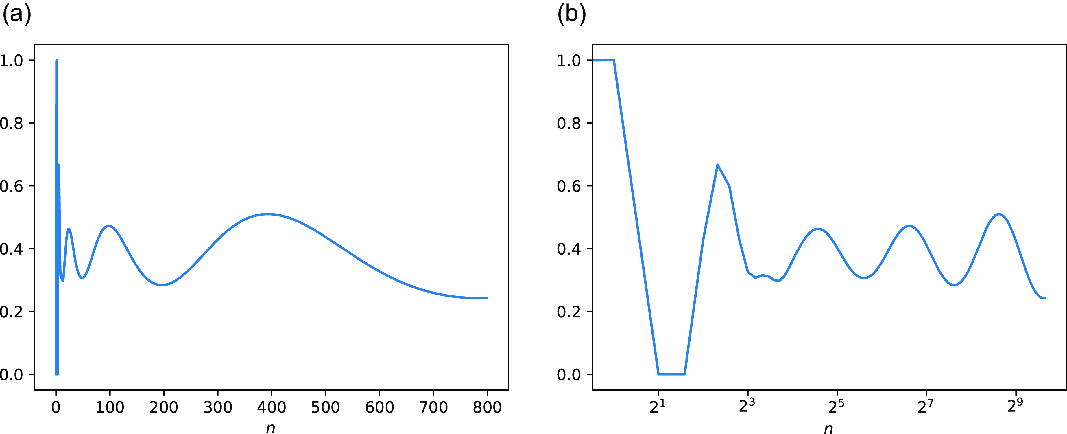
The first values of $\alpha_n \,:\!=\, \mathbb{E}\varphi_\alpha(\mathcal{P}_n)$ in the symmetric, binary case, on (a) a normal and (b) a logarithmic x scale, showing the oscillations.

We calculate $\alpha_n \,:\!=\, \mathbb{E}[\varphi_\alpha(\mathcal{P}_n)]$ for $0\leq n\leq N$ with $N\in\mathbb{N}$ . Then $\mathbb{E}[{\alpha(\mathcal{P}_n)}]$ can be bounded by

\begin{equation*}0 \le \mathbb{E}[ {\alpha(\mathcal{P}_n)}]- \Biggl({n + \sum_{k=2}^N \mathbb{E}[\varphi_\alpha(\mathcal{P}_k)]\mathbb{E}{[\Phi_k(\mathcal{P}_n)]}}\Biggr) \le \mathbb{E}[{\Phi_{>N}(\mathcal{P}_n)}].\end{equation*}

We can now use the simultaneous convergence of $\Phi_i$ and $\Phi_k, 2\leq k\leq N$ from Section 5.1. For $\Phi_{>N}$ we have $\Phi_{>N} = \Phi_{i} - \sum_{k=2}^N \Phi_k$ and the fact that the limits of $\mathbb{E}[\Phi_k], k\ge2$ sum up to the limit of $\mathbb{E}[\Phi_i]$ , and obtain in the $d_p=0$ case

(32) \begin{align}0 \le \lim_{n\to\infty}\dfrac{\mathbb{E}{[\alpha(\mathcal{P}_n)]}}n - \Biggl({1 + \sum_{k=2}^N \dfrac{(1-\rho(k))\alpha_k}{k(k-1)H}}\Biggr)&\le \sum_{k=N+1}^\infty \dfrac{1-\rho(k)}{k(k-1)H}\le \dfrac{1}{NH}.\end{align}

In the periodic $d_p>0$ case, the same can be done for each value of $f_{E,\alpha}^\ast$ .

The values $\alpha_k$ can be calculated by conditioning on the first step; this gives a recursive equation. For the symmetric, binary case, this is given by

\begin{equation*}\alpha_n = \sum_{k=1}^{n-1}\binom nk\dfrac{(1-\alpha_k)(1-\alpha_{n-k})}{2^n-2}\end{equation*}

for $n\ge2$ and $\alpha_1 = 1, \alpha_0=0$ . See Figure 1 for a plot of the first values of $\alpha$ . Calculating these values up to $N=800$ (higher values gave overflows in double-precision floats), we obtain from (32) the bounds

\begin{equation*}0.60225 < \dfrac 12+ \dfrac1{2H} f_{E,\alpha}^\ast({-}1) < 0.60316\end{equation*}

for the asymptotic mean of the proportion of essential nodes.