

Introduction
The biogeography of lichens is shaped by their sensitivity to a range of environmental drivers. At a regional-scale, patterns in lichen distribution are explained by sensitivity to pollution (Seaward Reference Seaward1998; Coppins et al. Reference Coppins, Hawksworth, Rose and Hawksworth2001), climatic gradients (Werth et al. Reference Werth, Tømmervik and Elvebakk2005; Giordani & Incerti Reference Giordani and Incerti2008) and habitat continuity (Tibell Reference Tibell1992; Selva Reference Selva1994). Often, the response of lichens has been ascribed to each of these drivers separately; consequently, lichen indices are developed for pollution loads (Hawksworth & Rose Reference Hawksworth and Rose1970; van Herk Reference Van Herk1999) and woodland history (Rose Reference Rose, Morris and Perring1974; Coppins & Coppins Reference Coppins and Coppins2002) or lichen indicators have been developed with which to examine possible climate change impacts (Ellis et al. Reference Ellis, Coppins, Dawson and Seaward2007). In reality, each of these environmental drivers may vary over space and time, either dependently or independently. For example, mandated pollution targets have, in general, lowered SO2-pollution, but N-deposition has increased (Woodin Reference Woodin1989; NEGTAP 2001); landscape management strategy is developing in response to emerging social-economic opportunities and environmental challenges (Rounsevell et al. Reference Rounsevell, Reginster, Araújo, Carter, Dendoncker, Ewert, House, Kankaanpää, Leemans and Metzger2006; Verburg et al. Reference Verburg, Rounsevell and Veldkamp2006); and the climate is changing (Jenkins et al. Reference Jenkins, Perry and Prior2007). Moreover, there may be important interactions between each of these drivers in controlling the overall lichen-response: for example, the response of lichens to climatic change may depend upon landscape-scale habitat quality (Ellis & Coppins Reference Ellis and Coppins2007; Ellis et al. Reference Ellis, Yahr and Coppins2009), as well as the pollution regime (Jovan & McCune Reference Jovan and McCune2005; Geiser & Neitlich Reference Geiser and Neitlich2007). It is therefore critically important to develop an integrated framework with which to understand the lichen-response to multiple environmental drivers. A first step in this process is to question the relative importance of contrasting drivers, and to partition their roles in explaining existing patterns of lichen assemblage composition and richness.
This paper describes a study which compiled and edited species record data that are freely available via the NBN Gateway (http://data.nbn.org.uk/) to examine the lichen response to three key environmental factors: climatic setting, pollution loads and woodland extent and continuity. We used multivariate ordination combined with least-squares regression to examine the relative importance of these competing factors in explaining lichen biogeographic patterns. This extends previously published analyses of NBN data (cf. Ellis et al. Reference Ellis, Yahr and Coppins2009; Ellis & Coppins 2010). However, this paper also explores the important implications of methodological differences. Modelling the species response to multiple variables belonging to different environmental drivers – i.e. many different climatic variables, or types of pollutant – presents a severe problem in predictive modelling, whereby spurious correlations may emerge as a consequence of the large number of potential explanatory variables. For individual species, models can be scrutinized for biological realism against a functional knowledge of the species' biology. In attempting to summarize the response of lichen communities, previous studies have compared species-assemblage data to summary gradients that were derived prior to the statistical comparison of environmental drivers (e.g. Ellis & Coppins Reference Ellis and Coppins2009, 2010). This approach has reduced many individual variables within a category (e.g. pollutants, climatic variables) to a single proxy gradient. This provides a useful generalization that avoids ‘over-parameterization’, including the possible emergence of misleading correlations through the input of many explanatory variables, though at the potential cost that important information may be lost during the development of summary gradients. As an alternative, in this study we used CCA to pre-select and then combine multiple individual variables simultaneously (without the a priori development of summary gradients), providing a complementary approach from which to develop new insights in the lichen response. Specifically, we ask: 1) what is the relative importance of climate, pollution, and woodland extent and continuity in controlling lichen composition and 2) how important are explanatory variables for composition in explaining patterns of species richness? Our analysis provides a preliminary summary of the general importance of regional environmental drivers for lichen biogeography in Scotland.
Methods
Field sites and species composition
Lichen presence-absence data were obtained for 324 woodland sites surveyed in Scotland by taxonomic specialists at the Royal Botanic Garden Edinburgh (RBGE) during the period 1972–2006 (data available from the British Lichen Society's Scottish Site Lichen Database via the National Biodiversity Network Gateway: http://data.nbn.org.uk/). All species were epiphytes sampled from tree bark or lignum.
Old-growth woodland
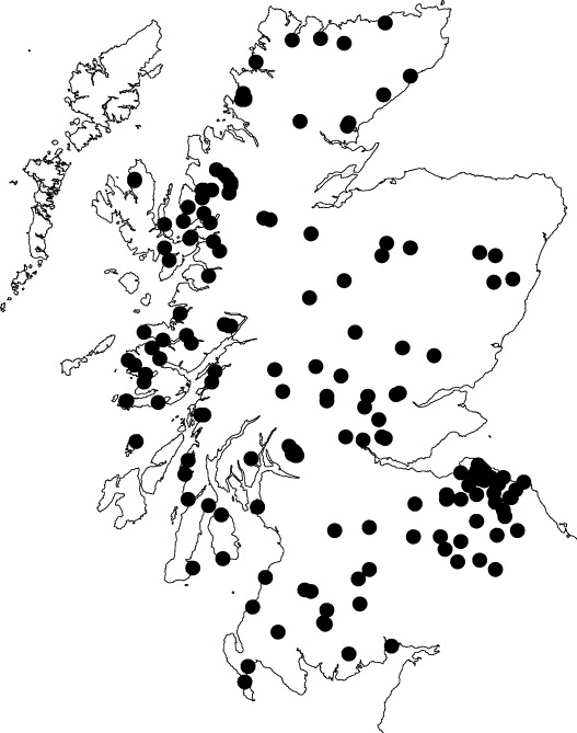
Individual woodland sites were compared to site-specific information on woodland temporal continuity using Scotland's Ancient Woodland Inventory (AWI: Walker & Kirby Reference Walker and Kirby1989; Roberts et al. Reference Roberts, Russell, Walker and Kirby1992). Geo-located lichen records and woodland stand histories from the AWI were compared to British Ordnance Survey 1:25 000 mapping (the O.S. ‘Explorer’ series) and the data were assessed for reliability. First, lichen records were grouped together if they were sampled from different stands (distinct woodland patches) within the same continuous woodland complex; second, woodlands were rejected if they comprised a large and complex mosaic of stands with different levels of continuity. On these criteria, a sub-set of 170 woodlands was identified as study sites, the edges of which were well delimited and which were of known antiquity (Fig. 1). Woodlands were characterized by the extent (ha) of habitat characterized as the progressive accumulation of woodland in each of four categories (cf. Walker & Kirby Reference Walker and Kirby1989; Roberts et al. Reference Roberts, Russell, Walker and Kirby1992): Class 1 = unbroken record of woodland cover since c. 1750; Class 2A = natural and semi-natural woodland stands with an unbroken record of woodland cover since c. 1870; Class 2B = planted woodland established before c. 1870; and Class 3 = planted woodland established after c. 1870, though on sites which were wooded in c. 1750.
Study-sites located across Scotland, sampled for lichen epiphyte communities.

Climate variables
Baseline climate data at a 5 km grid-square resolution were derived from UK Met Office modelled data-sets (Perry & Hollis Reference Perry and Hollis2005): estimated monthly and annual climatic averages for average, maximum and minimum monthly temperatures (°C) and precipitation (mm), including the number of days with > 1mm rainfall. Estimated climate data were verified against averages based on point data for the period 1961–2000 at 540 and 4 400 monitoring stations across Britain, for temperature and precipitation, respectively. A suite of fourteen climatic variables was calculated for individual 5 km grid-squares which contained study sites: mean annual temperature (°C), mean seasonal temperatures, temperatures of the warmest and coldest months of the year, annual temperature range, total annual precipitation (mm), seasonal precipitation and days > 1mm rainfall.
Pollution regime
The environmental loading of key pollutants was derived using modelled values at a 1 ha scale, using output specifically applicable to woodland and hedgerow habitats (NEGTAP, 2001; cf. www.apis.ac.uk): SO2 (μg m−3), acid deposition (keq ha−1 yr−1), nitrogen deposition (kgN ha−1 yr−1), ammonia (μg m−3), nitrogen oxides (μg m−3) and ozone (ppb hrs). Data were tested for normality and log-transformed when necessary (SO2, ammonia and nitrogen oxides).
Statistical analysis
Analysis of species composition was restricted to a sub-set of species with ≥ 5 records in the dataset. Variation in lichen composition was first mapped in ordination space using nonmetric multidimensional scaling based on a Sørenson dissimilarity matrix (NMDS; PC-Ord v 4.25, McCune & Mefford Reference McCune and Mefford1999). In an exploratory analysis, a random starting configuration was used to perform 40 data runs with a maximum of 400 iterations and an instability criterion equal to 0·00001. Default options were selected for remaining parameters (McCune & Mefford Reference McCune and Mefford1999). A Monte Carlo randomization test (50 randomized runs) was used to evaluate the statistical power of the exploratory analysis (McCune & Mefford Reference McCune and Mefford1999; McCune & Grace Reference McCune and Grace2002), and a final solution selected as a balance between low dimensionality, minimum stress [stress (S) ≈ fit between the rank order of samples in ordination space compared to an original dissimilarity matrix] and maximum stability (deviation in S over the preceding n iterations).
A second ordination was performed using detrended correspondence analysis (DCA). The unimodal assumption inherent in DCA was examined as the gradient length (= 6·33), which provides a measure of standard deviation in species turnover, with gradients < 3 pointing to linear response models as an alternative (Lepš & Šmilauer Reference Lepš and Šmilauer2003). In addition, DCA was tested by correlating DCA and NMDS axis scores. NMDS is not defined by an underlying model, but optimally maps in ordination space the variation between species and samples derived from a matrix of (dis)similarities. However, DCA and its derivatives (CCA, DCCA) are subject to the same underlying model – each of these ordination methods makes a strict assumption about the unimodal shape of the species-response. Økland (Reference Økland1999) suggested that ‘unexplained variation’ derived from correspondence analyses (DCA, CCA) may emerge from a lack-of-fit of field-data to the inherent response model. The comparison of NMDS and DCA may therefore be useful to examine the validity of DCA and its extensions (e.g. CCA) as a tool for ordination.
Canonical correspondence analysis (CCA) was used specifically to examine the relative importance of contrasting environmental drivers. Spatial terms derived using a cubic trend-surface of X-Y co-ordinates (Borcard et al. Reference Borcard, Legendre and Drapeau1992) were pre-selected using CCA, with Monte Carlo permutation tests (9999 randomizations) used to identify significant spatial components. Likewise, environmental variables were pre-selected for each environmental driver separately: i.e. selecting from amongst the variables describing climatic setting, pollution regime and woodland extent and continuity. Variance partitioning was used to identify the separate explanatory effect of spatial locality and environmental drivers combined. Variance partitioning was also used to investigate the effect of separate environmental drivers; this exercise was performed twice, with spatial locality included as a covariable, and then with spatial effects discounted from the analysis. Axis scores for CCA were compared to axis scores derived using NMDS and DCA, and the shift in correlation structure comparing NMDS-DCA, and NMDS-CCA, provides a rough measure of constraints imposed by regression against a limited suite of environmental variables.
The ‘full’ CCA model (incorporating all selected environmental variables) was contrasted with a ‘reduced’ model. This procedure was used to examine the robustness of the full model, for example, if each of the three environmental drivers (woodland extent and continuity, climatic setting and pollution regime) comprised different numbers of selected variables, it is possible that the variance explained may be artificially inflated for drivers with many component variables, compared to drivers with fewer selected variables (Peres-Neto et al. Reference Peres-Neto, Legendre, Dray and Borcard2006). The reduced model used variance partitioning, but with a maximum number of two component variables for each environmental driver, corresponding to the first two significant variables selected into CCA using Monte Carlo permutation (see above). Correspondence analysis was performed using CANOCO v. 4.5 (Ter Braak & Šmilauer Reference Ter Braak and Šmilauer2002; Lepš & Šmilauer Reference Lepš and Šmilauer2003). Ordination results were summarized as Venn diagrams, and presented as biplots for a limited range of species which were, a priori, expected to indicate contrasting environments:
1) oceanic lichens identified as old-growth indicator species by Ellis et al. (Reference Ellis, Yahr and Coppins2009),
2) species associated with the relatively more continental environment of north-east Scotland: identified as biogeographically restricted by Fryday (Reference Fryday, Shaw and Thompson2006), i.e. > 75% of their UK records (10 km scale) occurring in the Cairngorms, or as potential ‘boreal’ climatic indicators by Ellis et al. (Reference Ellis, Coppins, Dawson and Seaward2007), and
3) pollution indicators identified as ‘acidophytes’ or ‘nitrophytes’ by van Herk (Reference Van Herk1999) and Wolseley et al. (Reference Wolseley, James, Theobald and Sutton2006).
Multiple least-squares regression was used to compare species richness to the environmental variables selected to explain species composition. Analysis was performed using the MASS package (Venables & Ripley Reference Venables and Ripley2002) in R (2008), with forward and backward selection and AIC scores used to optimize a final regression model. The importance of selected variables was tested as the stepwise change in adjusted-R2, comparing a full regression model with a partial-model from which the respective variable had been removed.
Results
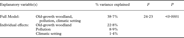
The trimmed dataset for analysis included 404 lichen species across 170 sites (Fig. 1). Ordination axes were correlated between NMDS and unimodal ordination using DCA, supporting the validity of correspondence analysis as an analytical framework (Table 1). Accordingly, CCA was used to model environmental factors selected as significant explanatory variables (Table 2). The relative importance of the three classes of drivers is statistically demonstrated with CCA, despite the modest amount of total variation explained by the model (see below).
Correlation-coefficients (r) between ordination axes derived using CCA, DCA and NMDS based on an optimal two dimensional solution: stress = 20·69; stability = 0·017; P < 0·05; axis one R2 = 0·532, axis two R2 = 0·226.

***P < 0·0001; **P <0·001; *P <0·05 (168 d.f.).
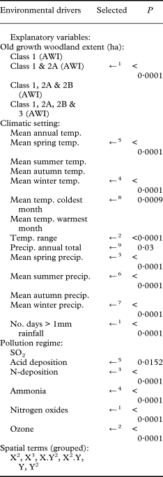
Environmental drivers and component explanatory variables used to describe the species composition of lichen epiphytes across 170 sites (cf. Fig. 1). Environmental variables are discriminated according to the order (x) in which they are selected into CCA (←x). Significance values (P) are derived using a Monte Carlo test with 9999 randomizations.

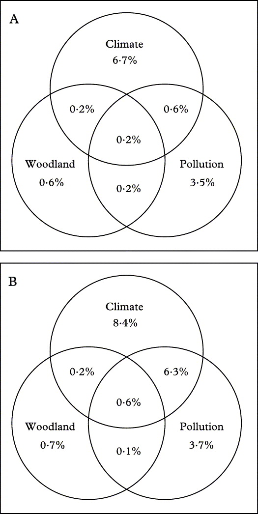
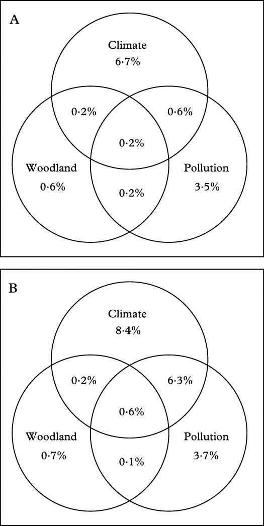
First, the combination of all selected spatial terms and environmental factors explained one quarter (24 %) of variation in the relationship between environmental-spatial and sample matrices. Treated by variance partitioning, the effect that was uniquely attributable to the spatial component explained one third of the variation in lichen composition compared to the environmental component (4 % compared to 12 %, respectively). Second, variance partitioning was used to compare contrasting environmental drivers – climatic setting, pollution regime and old-growth woodland extent – both with and without spatial terms as additional co-variables. With spatial terms included as covariables, environmental effects explained c. 12 % of variation in lichen composition (Fig. 2A); this increased to c. 20 % assuming that spatial patterns are wholly attributable to environmental gradients (Fig. 2B). In either case, the climatic setting explained a majority of variation in species composition, followed by the pollution regime and old-growth woodland extent (Fig. 2). Approximately equal proportions of the variance attributed to climatic setting were partitioned among temperature and rainfall variables (data not presented).
Venn diagrams showing partitioned variation in lichen composition explained by three landscape-scale drivers (CCA, full model): climate, pollution, and the extent of old-growth woodland. A, variance partitioned with spatial terms included as a co-variable (accounting for cross-correlation between spatial and environmental effects); B, variance partitioned with spatial terms discounted from the analysis (assuming spatial variation is wholly attributable to environmental gradients). In all cases partial-CCA solutions were significant, P < 0·0001 (Monte Carlo test with 9999 permutations).
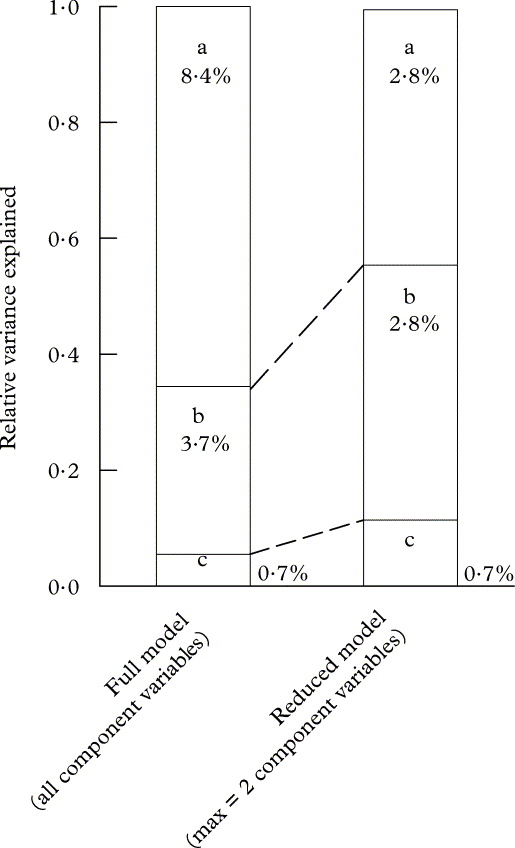
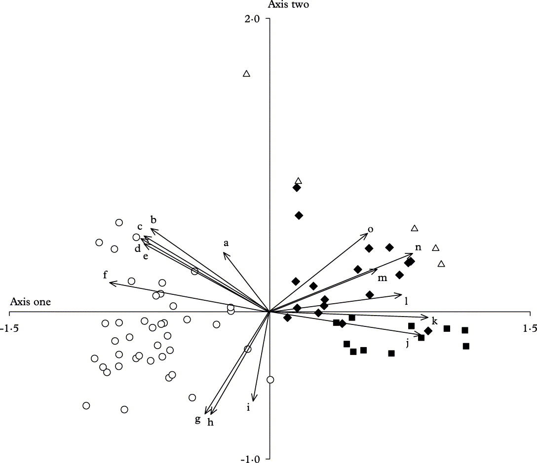
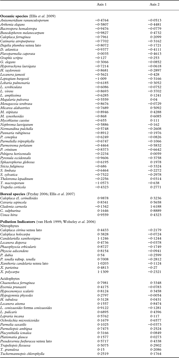
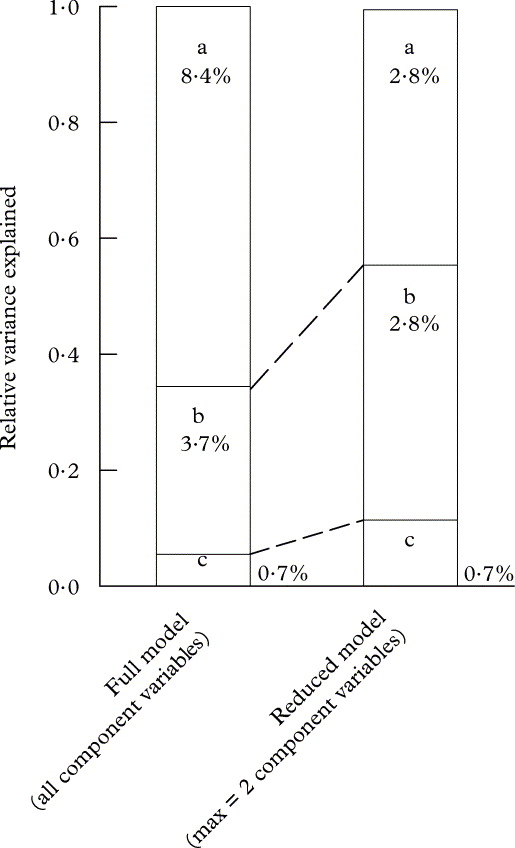
We tested for the possible over-parameterization of our optimum model, especially the occurrence of inflation in the partitioned variance if more explanatory variables are available for the characterization of certain environmental drivers, compared to others. Our test compared the full model (all selected variables for each environmental driver) against a reduced model (maximum of two variables for each driver). For climatic setting the reduced model was restricted to the number of days > 1 mm rainfall and temperature range, and for pollution, values of NOx and ozone (Table 2). This approach shifted the relative importance of climate with respect to the pollution regime (Fig. 3); they became more similar under a reduced model. Therefore, taking a circumspect approach to the full model: 1) CCA sample scores were significantly correlated with NMDS axes (Table 1), suggesting that the selected explanatory variables provide a representation of the processes structuring epiphyte composition, and 2) equivalent patterns of species composition are consistent with previous evidence from British lichen biogeography, i.e., suites of putative indicator species for contrasting environmental conditions demonstrated a consistent relationship with the selected environmental drivers (Fig. 4). In a two-dimensional system the extent of old-growth woodland and precipitation co-varied, reflecting possible interaction between the climatic setting and habitat quality for oceanic epiphytes, while pollution regime co-varied with the temperature range, such that boreal epiphytes and pollution indicators were spatially associated in the ordination plot.
Stacked bar-charts to compare the relative variance explained by three environmental drivers (cf. Figure 2B). a, climatic setting; b, pollution regime; c, woodland extent and continuity. Differences between the stacks compare the variance explained by a full model (with all selected variables included) and a reduced model, limited to a maximum of two selected variables for each environmental driver. Values of percent variation explained are shown with their respective bars.
Ordination-plot for the results of CCA (full model) to summarize the relationship between selected environmental factors (cf. Table 2) and contrasting indicator species groups (cf. Appendix 1): ○ = oceanic species, ▵= boreal species, ■ = nitrophytes, ♦ = acidophytes. Canonical axes were significant, P < 0·001 (Monte Carlo test with 9999 randomizations). Vectors for environmental factors: a, extent of old-growth woodland; b, spring precipitation; c, winter precipitation; d, total precipitation; e, summer precipitation; f, days > 1 mm; g, winter temperature; h, minimum temperature; i, spring temperature; j, ammonia; k, nitrogen oxide; l, N-deposition; m, acid deposition; n, temperature range; o, ozone.

Of the environmental factors selected to explain species composition (Table 2), four variables were selected in an optimum model for species richness: old-growth woodland extent (for natural and semi-natural woodland since c. 1870), acid deposition, N-deposition and winter temperature. Using variance partitioning, the importance of drivers in explaining richness decreased in the order: old-growth extent > pollution > climate (Table 3).
Discussion
This study aimed to explore the role of contrasting environmental drivers in controlling lichen epiphyte composition and richness. To do this we used a large-scale floristic database, combined with modelled data for climate and pollution, and cartographic data for woodland extent and continuity. Floristic databases are problematic because they are frequently subjective and not systematically sampled. To overcome this problem we restricted our analysis to sites that had been comprehensively sampled by the second author (BJC), providing a degree of conformity. A second problem emerges because environmental data were modelled at contrasting scales: 5 km grid-scale for climate, 1 ha grid-scale for pollution, and site-specific measures for woodland parameters. Data interpretation is therefore based on the nested effect of pollution within the macroclimatic setting, with reference to the central point within a woodland sampling site. Delimited woodland sites were quantified in terms of their extent and temporal continuity, and smaller-scale effects, for example, local topography, tree species composition and age-structure, were therefore discounted, weakening the possible explanatory role of trends in woodland habitat. We would nevertheless argue that our scenario is a reasonable approximation for modelling at a regional-scale, and that the cautious application of large-scale datasets may be justified so long as these potential sources of model variability are clearly recognized and stated.
Drivers of species richness: richness is partitioned into components explained independently by selected variables, corresponding to each of the three regional environmental drivers: old-growth woodland extent (Class 1 & 2A AWI categories), pollution regime (acid deposition and N-deposition) and climate setting (winter temperature). Results of multiple least-squares regression (AIC optimized).

Modelling the response of species and communities to environmental drivers is a difficult balance between the risk of over-parameterization, and allowing model flexibility. In this study we explored lichen community structure with respect to a total of 21 environmental and spatial drivers (full model), which were selected for significance using permutation tests. This contrasts with a previous study using equivalent data, which collapsed variables describing contrasting environmental drivers into summary gradients (Ellis & Coppins 2010; see also Ellis & Coppins Reference Ellis and Coppins2009). The important contrast as a consequence of these methodological differences is the suggestion that local macroclimatic setting (5 km scale) may have a relatively more important effect on species composition than was previously indicated. The use of a reduced model to test for the excessive parameterization of certain environmental drivers reduced differences in the relative importance of climatic setting and the pollution regime, though continued to support the importance of climatic setting as a key driver for epiphyte composition. The importance of climate relative to pollution is broadly consistent with the observation that Scotland is a relatively clean-air environment both within the British Isles and compared to Europe more widely (NEGTAP 2001). This dominant effect of climate in Scotland may also be explained by steep climatic gradients, which have been previously shown to structure lichen communities (Ellis & Coppins Reference Ellis and Coppins2006; Ellis et al. Reference Ellis, Coppins, Dawson and Seaward2007).
Despite contrasts between modelling protocols (including all variables in a full model, restriction into a reduced model, or the use of single proxy gradients), the central message of the contrasting analyses remains the same. First, our study underscores the assertion that the predictive biogeographic analysis of lichen communities would benefit from the consideration of multiple drivers. Studies focusing on species distributions with respect to single environmental drivers represent an incomplete picture of the processes controlling lichen distribution. Second, our results indicate that the relative importance of environmental drivers may shift between the consideration of species composition, and species richness. Thus, at a regional-scale for Scotland, species composition is expected to be controlled, in order of importance, by climatic setting > pollution regime > old-growth woodland extent. In contrast, species richness is controlled by old-growth woodland extent > pollution regime > climatic setting. This shift represents an important functional decoupling between lichen species composition and richness for our system (cf. Keppel et al. Reference Keppel, Buckley and Possingham2010 for a decoupling scenario in an alternative system).
It has been demonstrated that lichen epiphyte composition changes along climatic gradients with respect to species' functional traits, such that cyanolichens (e.g. requiring liquid water for photosynthesis: Lange et al. Reference Lange, Kilian and Ziegler1986, Reference Lange, Büdel, Meyer and Kilian1993) and species in genera with tropical affinities [e.g., Graphis: Staiger & Kalb (Reference Staiger, Kalb, Nash, Ryan, Diederich, Gries and Burgartz2004); Thelotrema: Frisch (Reference Frisch2006); Hypotrachyna: Louwhoff (Reference Louwhoff2001); Parmotrema: Louwhoff (Reference Louwhoff2001)] are associated with oceanic climates (Green & Lange Reference Green and Lange1991; Ellis et al. Reference Ellis, Yahr and Coppins2009), including along Scotland's Atlantic west coast: cf. Appendix 1 and Fig. 4. In contrast, a suit of ‘boreal’ or ‘continental’ species occur in eastern Scotland, where the climate is cooler in winter, warmer in summer (i.e. with greater temperature range), and is drier with less consistent rainfall: for example Cetraria sepincola, Cladonia carneola and Usnea hirta (cf. Appendix 1 and Fig. 4). Likewise, species response to pollution is well documented (Coppins et al. Reference Coppins, Hawksworth, Rose and Hawksworth2001; van Dobben et al. Reference Van Dobben, Wolterbeek, Wamelink and Ter Braak2001). Species composition shifts along pollution gradients, such that species more tolerant of N-pollution are increasingly prevalent at sites towards Scotland's urban or industrial centres, or in intensively agricultural settings: for example Physcia spp., and Xanthoria spp. (cf. Appendix 1 and Fig. 4). As pollution loads increase, the number of species with a threshold tolerance declines, and pollution therefore has a dual effect on composition and richness (cf. Tables 2 & 3). In contrast, a small number of species are obligate old-growth indicators, and occur almost exclusively in old-growth woodlands (e.g. Coppins & Coppins Reference Coppins and Coppins2002; Ellis et al. Reference Ellis, Yahr and Coppins2009). These old-growth elements represent a sub-set of total lichen richness, with limited potential to skew overall trends in species composition. Previous studies have suggested that niche specialists or dispersal-limited species are more likely to occur in old-growth woodlands (Sillett et al. Reference Sillett, McCune, Peck, Rambo and Ruchty2000; Gignac & Dale Reference Gignac and Dale2005; Löbel et al. Reference Löbel, Snäll and Rydin2006), though occurrences of such species may be generated from across a wide spectrum of potential colonists (e.g. many lichens might be considered niche specialists), weakening the power of old-growth woodland as an explanatory factor for compositional trends.
The property of old-growth woodland of accumulating a wide spectrum of niche-specialist or dispersal-limited species has a strong effect on species richness. The specific effect of old-growth woodland extent could be explained both in terms of population dynamics, with respect to increased colonization likelihoods with habitat continuity (Sillett et al. Reference Sillett, McCune, Peck, Rambo and Ruchty2000; Löbel et al. Reference Löbel, Snäll and Rydin2006), or as an increase in environmental heterogeneity with woodland area (Berglund & Jonson Reference Berglund and Jonsson2001; Gignac & Dale Reference Gignac and Dale2005) and therefore increased opportunity for colonization by niche specialists. A key point of our results is that composition may change with respect to climate, while levels of richness are buffered by habitat conditions, that is, considering temporal shifts in climate (e.g. climate change scenarios), there may be a turnover in species composition, though patterns of species richness may continue to reflect underlying trends in habitat quality. This critical distinction between the compositional response to climate described by bioclimatic models, and species richness with respect to habitat quality, may be poorly resolved by studies which seek to contrast directly the effect of climate and habitat quality on local richness patterns (Moning et al. Reference Moning, Werth, Dziock, Bässler, Bradtka, Hothorn and Müller2009). Even at regional scales (e.g. across Scotland) it is not necessarily surprising that climate has little direct explanatory power for patterns of richness within a given habitat-type; the scale of analysis is too small for a functional climatic effect on richness patterns, for example, the positive relationship between species richness and gradients in thermal energy and water regime (Currie Reference Currie1991; Hawkins et al. Reference Hawkins, Field, Cornell, Currie, Guégan, Kaufman, Kerr, Mittelbach, Oberdorff and O'Brien2003). Threats to epiphyte species may nevertheless emerge from the interplay between drivers for composition and richness. For example, the smaller-scale effect of microclimate may be important in off-setting the putative importance of macroclimate as a force for species turnover (e.g. Lidén & Hilmo Reference Lidén and Hilmo2005). However, without strong micro-habitat buffering, climate impacts on lichens may occur indirectly as a consequence of habitat loss and fragmentation (cf. Travis Reference Travis2003). Thus, rapid macroclimatic change presents the possibility for increasing population extinction rates, and lowered establishment rates, for sensitive range-edge species. If the net rates of population loss for existing species are not matched by dispersal or establishment rates for colonizers adapted to contrasting climatic settings, species-rich habitats may indeed lose species, though this would occur as an indirect consequence of climate change, related to population dynamic processes in fragmented habitats.
In summary, our analysis provides support for the general principle that lichen biogeography and conservation would benefit from an integrated predictive understanding of multiple environmental drivers. This is an important consideration with respect to climate change impacts, pollution, and habitat management, which are too frequently considered as separate issues. Considering multiple drivers has the benefit of providing comprehensive opportunities for regional-scale management, for example, driving down pollution loads may render old-growth woodland newly available for lichen epiphyte colonization, possibly buffering the effect of climate impacts. A more integrated approach thus provides opportunities to develop a more effective conservation strategy, by identifying synergies or conflicts between separate pieces of legislation and policy. However, integrating across the multiple variables which comprise each of the large-scale drivers holds significant challenge. Different approaches, a priori collapsing the drivers to summary gradients compared to selection from amongst a large number of individual variables, may subtly shift the relative importance of drivers in explaining the lichen community response. No single modelling procedure is likely to provide a definitive answer or predictive outcome, and we suggest accordingly there is strength in using different approaches to identify a consensus, while testing the compatibility of results with multi-disciplinary evidence from observation and experimentation.
This work is an RBGE core-funded project, supported as grant-in-aid through the Scottish Government's Rural and Environment Research and Analysis Directorate. We thank Dr Susan Will-Wolf and two anonymous referees for comments which improved the draft manuscript.
Canonical correspondence axis scores for an a priori selection of indicator species, plotted onto Figure 4.