2.1. Specification

In insurance pricing and claims models, the misrepresentation of risk factors presents a significant challenge that can result in inaccurate premium calculations and inappropriate claim payments. Traditional statistical models typically presume that these risk factors are reported accurately; however, policyholders may intentionally conceal or misrepresent adverse information to secure lower premiums or higher payouts. Consequently, the development of models that can address and rectify the biases introduced by such misrepresentations is a critical objective in the insurance sector.

In our analysis, in addition to the conventional covariates, we introduce a binary risk factor v that is subject to misrepresentation. For this predictor, we assume that $v=0$ corresponds to an outcome favorable to the individual (i.e. lower premium), whereas $v=1$ leads to an unfavorable result. Due to the misstatement on this risk factor, we denote $v^{\ast}$ to be the observed and reported status. Under the assumption of unidirectional misrepresentation, we have the following relationships:

(2.1) \begin{equation}\Pr(v=1|v^{\ast}=1)=1, \quad \Pr(v=1|v^{\ast}=0)=q, \quad 0 \lt q \lt 1,\end{equation}

where q is referred to as the prevalence of misrepresentation (Akakpo et al., Reference Akakpo, Xia and Polansky2019). It is further assumed that, conditional on the true status v, the response variable y is independent of the reported status $v^{\ast}$. The probability function that accounts for misrepresentation then becomes:

(2.2) \begin{equation}f_Y(y|\boldsymbol{x},v^{\ast})=\big[f_1(y)\big]^{v^{\ast}}\left[q f_1(y)+(1-q)f_0(y)\right]^{1-v^{\ast}}\!,\end{equation}

where

(2.3) \begin{align}f_1(y) &= f_{Y}(y|\boldsymbol{x},v=1),\end{align}

(2.4) \begin{align}f_0(y) &= f_{Y}(y|\boldsymbol{x},v=0),\end{align}

and $\boldsymbol{x}=(x_{1},\ldots, x_{p})^\top$ denotes the covariate set.

The quantity of interest in our model is the log-transformed claim severity. In the linear framework, we assume that it follows a normal distribution, which aligns with the characteristics of the data and facilitates the analysis. The mean parameter $\mu$ of the normal distribution is incorporated into the model through an identity link function:

(2.5) \begin{equation}\mu=\beta_0+\boldsymbol{x}^\top \boldsymbol{\beta}+\beta_v v,\end{equation}

where $\beta_0$, $\boldsymbol{\beta}=(\beta_1,\ldots,\beta_p)^\top$ and $\beta_v$ represent the corresponding regression coefficients. We assume that the variance $\sigma^2$ of the normal distribution is known; otherwise, it can be inferred from the data. To explore the potential impact of predictors on the prevalence parameter q, covariates can be included in q using a logit link function:

(2.6) \begin{equation}q=\frac{\exp\big(\alpha_0+\boldsymbol{x}^\top \boldsymbol{\alpha}\big)}{1+\exp\big(\alpha_0+\boldsymbol{x}^\top \boldsymbol{\alpha}\big)},\end{equation}

where $\boldsymbol{\alpha}=( \alpha_1,\ldots,\alpha_p)^\top$.

The individual likelihood function is then given by

(2.7) \begin{equation} L_i(\boldsymbol{\Theta};\, y_i, \boldsymbol{x}_i, v_i^{\ast}) = \left[f_1(y_i)\right]^{v_i^{\ast}}\left[q_i f_1(y_i)+(1-q_i)f_0(y_i)\right]^{1-v_i^{\ast}},\end{equation}

where $\boldsymbol{\Theta}=\{\beta_0, \boldsymbol{\beta}, \beta_v, \alpha_0, \boldsymbol{\alpha}\}$ represents the parameter set to be estimated.

2.2. High-dimensional modeling

The model specification above provides a flexible framework for accommodating misrepresentation in claims data. However, when the number of covariates p is large, the inclusion of all predictors in both the mean and prevalence components may lead to overfitting and diminished interpretability. Moreover, not all covariates necessarily influence the misrepresentation behavior or the claim severity, motivating the need for variable selection. To this end, we adopt a penalized likelihood approach that simultaneously performs parameter estimation and variable selection. Specifically, we impose $L_1$ penalty terms on the coefficients in both the mean and prevalence components, which encourage sparse solutions by shrinking irrelevant coefficients to zero. This formulation enables us to identify key risk factors that affect claim severity and those that drive misrepresentation behavior, while maintaining model parsimony in high-dimensional settings. The overall optimization problem is formulated as:

(2.8) \begin{equation}\mathop{\text{minimize}} \limits_{\boldsymbol{\Theta}} -\frac{1}{N} \sum_{i=1}^{N} \log L_i(\boldsymbol{\Theta};\, y_i, \boldsymbol{x}_i, v_i^{\ast}) + \lambda_Q \sum_{j=1}^{p} |\alpha_j| + \lambda_Y \sum_{j=1}^{p} |\beta_j|,\end{equation}

where $\lambda_Q$ and $\lambda_Y$ are tuning parameters. The misrepresented risk factor v is considered a significant predictor, and therefore, no penalty is applied to $\beta_v$ to retain it in the model. For conciseness, the corresponding estimation procedure is provided in Appendix A.

3.1. Overview of DNN

We briefly review the DNN architecture. Let L be the number of hidden layers, and $n_l$, $l=0,\ldots,L+1$, be the number of neurons in each layer. Here, $n_0$ and $n_{L+1}$ correspond to the dimensions of the input and output layers, respectively. Let $\sigma(\!\cdot\!)$ denote the activation function in the hidden layers, and $\psi(\!\cdot\!)$ denote the activation function in the output layer. We define $\boldsymbol{W}^{(l)} \in \mathbb{R}^{n_l \times n_{l-1}}$ and $\boldsymbol{b}^{(l)} \in \mathbb{R}^{n_l}$, $l=1,\ldots,{L+1}$ as the weight matrix and bias term, respectively. The total parameter set of the neural network is denoted by $\boldsymbol{\Theta}=\{\boldsymbol{W}^{(l)}, \boldsymbol{b}^{(l)}:\, l=1,\ldots,L+1 \}$. For clarity, we treat $\boldsymbol{\Theta}$ as a column vector in $\mathbb{R}^m$, where $m=\sum_{l=1}^{L+1} n_l\left(n_{l-1}+1\right)$.

To delve into the mathematical description of the DNN, we can break down its structure starting from the input layer and progressing towards the output layer:

(3.1) \begin{align}\boldsymbol{a}^{(1)} &= \boldsymbol{W}^{(1)}\boldsymbol{x}+\boldsymbol{b}^{(1)}, \quad\boldsymbol{z}^{(1)} = \sigma\big(\boldsymbol{a}^{(1)}\big), \end{align}

(3.2) \begin{align}\kern5.1pc\quad \boldsymbol{a}^{(l)} &= \boldsymbol{W}^{(l)} \boldsymbol{z}^{(l-1)}+\boldsymbol{b}^{(l)}, \quad\boldsymbol{z}^{(l)} = \sigma\big(\boldsymbol{a}^{(l)}\big), \quad l=2,\ldots,L,\end{align}

(3.3) \begin{align}\kern2.8pc \boldsymbol{a}^{(L+1)} &= \boldsymbol{W}^{(L+1)} \boldsymbol{z}^{(L)}+\boldsymbol{b}^{(L+1)}, \quad\boldsymbol{z}^{(L+1)} = \psi\big(\boldsymbol{a}^{(L+1)}\big).\end{align}

The choice of the output activation function $\psi(\!\cdot\!)$ should be aligned with the specific problem being tackled. For the binary classification problem, a sigmoid function $\psi(a)=1 /(1+\exp (-a))$ can be implemented; for the regression problem, an exponential or identity function can be applied.

3.2. DNN with misrepresentation

To effectively address the challenges associated with misrepresentation, we propose a modeling approach utilizing DNN. We define two neural networks, $\text{NN}_Y$ and $\text{NN}_Q$, to model the log-transformed claim severity $y_i$ based on $ (\boldsymbol{x}_i,v_i) $, and the probability of misrepresentation $q_i$ for individuals with $ v_i^* = 0 $ based on the features $ \boldsymbol{x}_i$, respectively. The final output of the overall neural network, which integrates $\text{NN}_Y$ and $\text{NN}_Q$, is as follows:

(3.4) \begin{equation}\mu ( \boldsymbol{x}_i, v^*_i;\, \boldsymbol{\Theta} ) =\begin{cases}\mu_Y ( \boldsymbol{x}_i, v_i = 1;\, \boldsymbol{\Theta}_Y), & v_i^* = 1, \\\mu_Q ( \boldsymbol{x}_i;\, \boldsymbol{\Theta}_Q) \mu_Y ( \boldsymbol{x}_i, v_i = 1;\, \boldsymbol{\Theta}_Y) + ( 1 - \mu_Q ( \boldsymbol{x}_i;\, \boldsymbol{\Theta}_Q) ) \mu_Y ( \boldsymbol{x}_i, v_i = 0;\, \boldsymbol{\Theta}_Y), & v_i^* = 0,\end{cases}\end{equation}

where $\boldsymbol{\Theta}=\{\boldsymbol{\Theta}_Q,\boldsymbol{\Theta}_Y\}$, $\mu_Y$ is the final output from $\text{NN}_Y$, and $\mu_Q$ is the final output from $\text{NN}_Q$.

The proposed loss function is defined as

(3.5) \begin{equation}\mathcal{L}( \boldsymbol{\Theta} )=\frac{1}{N}\sum\limits_{i = 1}^N \ell_0 ( y_i,\mu ( \boldsymbol{x}_i, v_i^*;\, \boldsymbol{\Theta} ) ) + \omega \operatorname{KL}(\bar{\mu}_{Q}||\varepsilon),\end{equation}

which consists of two key components: a standard prediction loss and a regularization term that penalizes deviations from a baseline assumption of honesty. The first term measures the prediction accuracy using squared error loss, defined as $\ell_0(y, \mu)=(y-\mu)^2$. The second term imposes a KL divergence constraint defined as:

(3.6) \begin{equation} \operatorname{KL}(\bar{\mu}_{Q}||\varepsilon) = \bar{\mu}_{Q} \log\left(\frac{\bar{\mu}_{Q}}{\varepsilon}\right) + (1-\bar{\mu}_{Q}) \log\left(\frac{1-\bar{\mu}_{Q}}{1-\varepsilon}\right)\!,\end{equation}

where $\bar{\mu}_{Q}$ denotes the average predicted misrepresentation probability for the subgroup with $v_i^* = 0$, and $\varepsilon \gt 0$ is a small fixed constant that anchors the KL divergence to a baseline of near-zero misrepresentation probability. The regularization strength is governed by the tuning parameter $\omega$, which is selected via validation. By setting $\varepsilon$ to a small constant (e.g., $10^{-6}$), this KL divergence regularization induces sparsity in the latent misrepresentation variables. When data provide limited evidence of misrepresentation, this term penalizes deviations from the baseline and drives $\text{NN}_Q$ outputs toward zero, implementing a default honesty assumption. When empirical evidence is sufficiently strong, the data-fitting term overrides this anchor, allowing the model to detect genuine misrepresentation.

3.3. Sparse-input deep neural network

To perform variable selection in a DNN, we propose fitting a sparse-input deep neural network (SIDNN) by applying an $L_1$-gMCP to the weights connecting the input layer to the first hidden layer. The inclusion of this type of penalty term facilitates variable selection in neural networks. Let $w_{jk}^{(1)}$ represent the element in the j-th row and k-th column of $\boldsymbol{W}^{(1)}$. The parameters of the neural network can then be estimated by solving the following optimization problem:

(3.7) \begin{equation} \mathop {\arg \min }\limits_{\boldsymbol{\Theta}} \left\{ \mathcal{L}_0(\boldsymbol{\Theta}) + P\left(\boldsymbol{W}^{(1)};\, \lambda ,\gamma \right) \right\},\end{equation}

where $\mathcal{L}_0(\boldsymbol{\Theta})$ denotes a general loss function, and

(3.8) \begin{equation}P\left(\boldsymbol{W}^{(1)};\, \lambda ,\gamma \right)=\sum_{k = 1}^{n_0} \rho \left( {\sum\nolimits_{j = 1}^{n_1} \left| w_{jk}^{(1)} \right|\!;\, \lambda ,\gamma} \right)\!,\end{equation}

with $\rho ( t;\, \lambda ,\gamma )=\lambda\int_0^{|t|}(1-\frac{x}{\gamma \lambda})_{+} \mathrm{d}x$ as the MCP function.

The $L_1$-gMCP combines the group MCP with the LASSO penalty. The outer MCP promotes sparsity at the input layer by constraining the entire vector $w_{\cdot k}^{(1)}=(w_{1k}^{(1)}, \ldots, w_{n_{1}k}^{(1)})^\top$ to be zero, thus facilitating variable selection. The inner LASSO penalty further promotes sparsity by forcing some of the individual weights $w_{jk}^{(1)}$ to be zero. The parameter $\lambda$ governs the strength of the penalty, thus influencing the sparsity of the model. 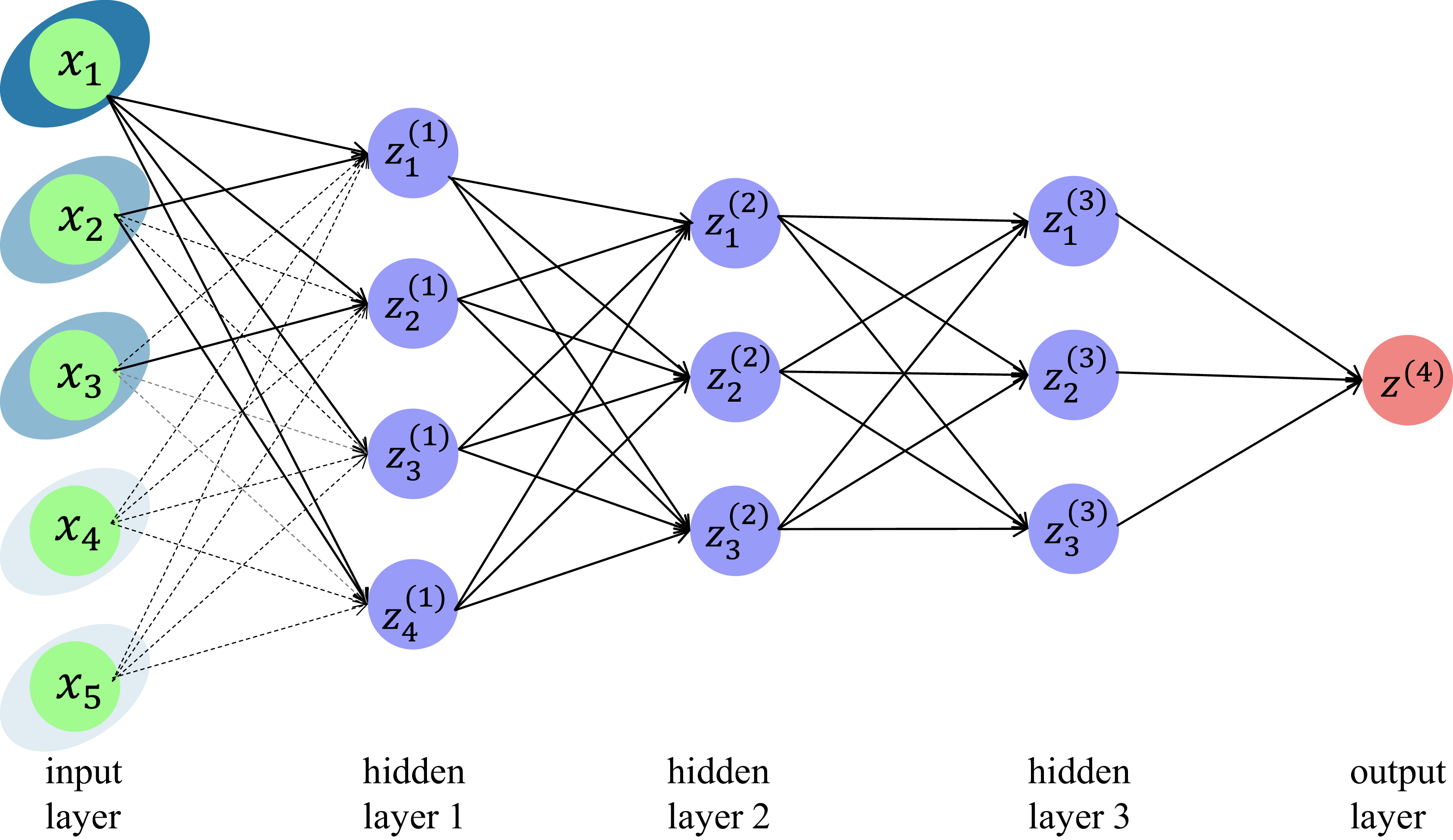Meanwhile, the parameter $\gamma$ regulates the concavity of the penalty function, helping to balance bias and variance. Figure 1 illustrates how the penalty term in (3.7) operates.

Figure 1.

An example of a sparse-input neural network, specifically a four-layer deep neural network with architecture $\boldsymbol{m}=(5, 4, 3, 3, 1)$. The heavy and dotted lines indicate nonzero and zero weights, respectively. Each shaded oval corresponds to a group of first-layer weights. The weights from the dark blue oval are both nonzero. Each medium blue oval contains a subset of nonzero weights, thereby exhibiting element-wise sparsity. All the weights in the light blue ovals are zero, so they exhibit group-level sparsity.

3.4. SIDNN with misrepresentation

To achieve variable selection within the neural network framework addressing the misrepresentation problem, we introduce $L_1$-gMCP regularization terms in both $\text{NN}_Y$ and $\text{NN}_Q$. The optimization problem can be formulated as follows:

(3.9) \begin{equation}\mathop {\arg \min }\limits_{\boldsymbol{\Theta}} \left\{\mathcal{L}(\boldsymbol{\Theta}) + \sum_{\mathcal{A} \in \{Y,Q\}} P\left( \boldsymbol{W}^{(1)}_{\mathcal{A}};\, \lambda _{\mathcal{A}}, \gamma _{\mathcal{A}} \right) \right\}\!,\end{equation}

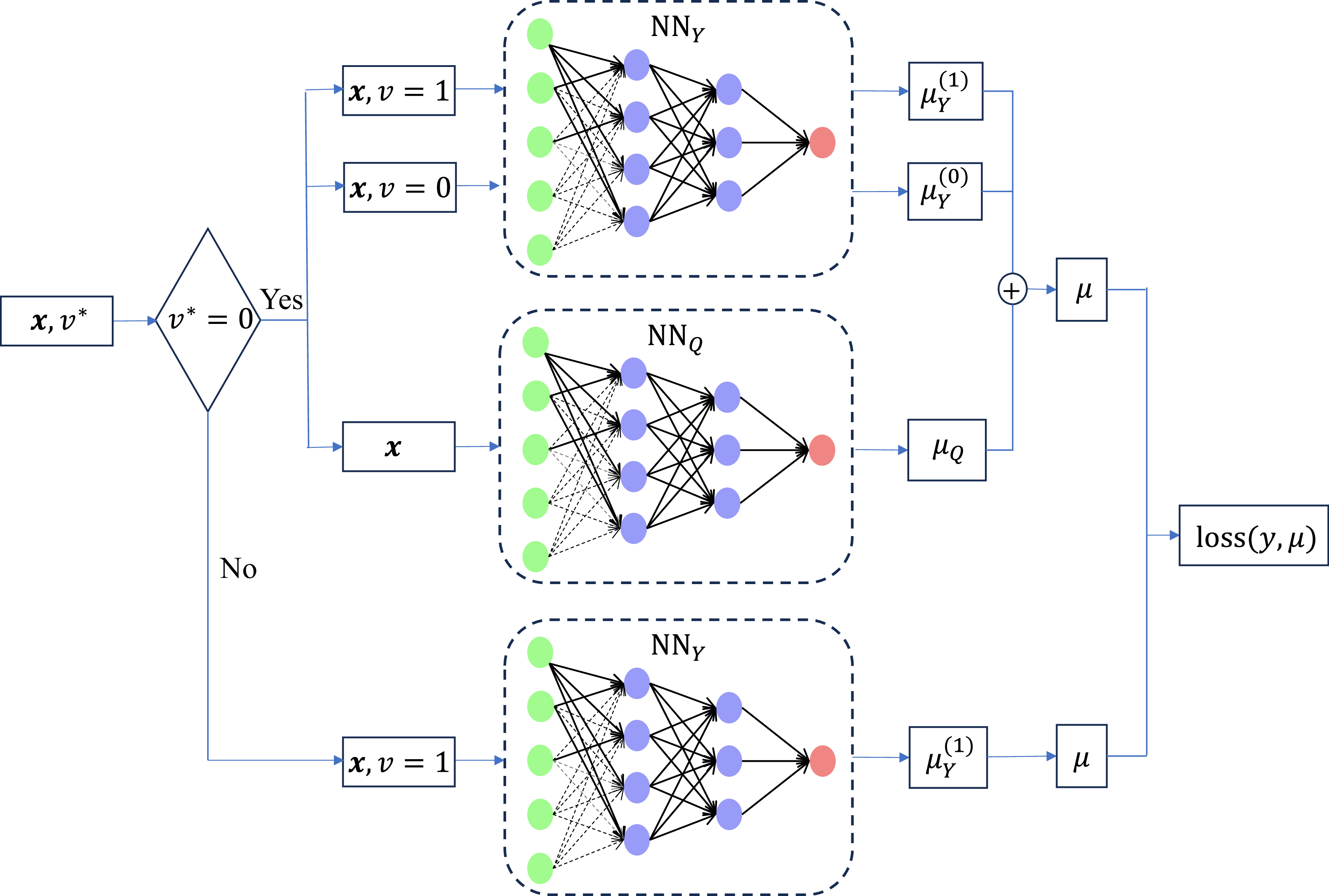
where $\mathcal{L}(\boldsymbol{\Theta})$ is defined in (3.5), and the penalty term is the same as in (3.8). The symbol $\mathcal{A}$ denotes the corresponding neural network. Note that v is considered a significant factor in our model, and thus no penalty is applied to the weights associated with v. Specifically, $\boldsymbol{W}^{(1)}_{Y}$ excludes the weights corresponding to edges connected to v. The overall structure of our neural network is depicted in Figure 2.

Figure 2.

SIDNN-based claims model with misrepresentation adjustment.

3.5. Learning

The objective function in (3.9) includes a non-smooth regularization term, which makes it unsuitable for direct optimization via gradient descent. To address this, we utilize the PGD method to obtain a sparse solution for the parameters. By initially applying the LLA technique, we transform the original $L_1$-gMCP problem into an adaptive LASSO problem, and then compute its proximal solution (Zou and Li, Reference Zou and Li2008).

3.5.1. LLA of $L_1$-gMCP

Given the value of $w_{\mathcal{A},jk}^{(1)}$ at iteration t, the LLA of the penalty term $P( \boldsymbol{W}^{(1)}_{\mathcal{A}};\, \lambda _{\mathcal{A}}, \gamma _{\mathcal{A}})$ at $|w_{\mathcal{A},jk}^{(1)}| = |w_{\mathcal{A},jk}^{(1),t}|$ is:

(3.10) \begin{equation}P\left( \boldsymbol{W}^{(1)}_{\mathcal{A}};\, \lambda_{\mathcal{A}}, \gamma _{\mathcal{A}} \right) \approx \sum_{k=1}^{n_{0}^{\mathcal{A}}} \sum_{j=1}^{n_{1}^{\mathcal{A}}} \delta_{\mathcal{A},k}^{t} \left| w_{\mathcal{A},jk}^{(1)} \right| + C_0,\end{equation}

where $C_0$ is a constant that does not depend on $|w_{\mathcal{A},jk}^{(1)}|$, and $\delta_{\mathcal{A},k}^{t}$ is the first-order partial derivative of $P( \boldsymbol{W}^{(1)}_{\mathcal{A}};\, \lambda_{\mathcal{A}}, \gamma _{\mathcal{A}})$ evaluated at $|w_{\mathcal{A},jk}^{(1),t}|$, given by:

(3.11) \begin{equation}\delta_{\mathcal{A},k}^{t} = \left( \lambda _\mathcal{A} - \frac{\sum_{j=1}^{n_{1}^{\mathcal{A}}} \left| w_{\mathcal{A},jk}^{(1),t} \right|}{\gamma_\mathcal{A}} \right)_{+},\end{equation}

where ${{\left( x \right)}_{+}} = \max \left( x, 0 \right)$. Note that $n_{0}^{Y}=n_{0}^{Q}=p$ represents the dimension of the input features $\boldsymbol{x}$, while $n_{1}^{Y}$ and $n_{1}^{Q}$ denote the number of neurons in the first hidden layers of $\text{NN}_Y$ and $\text{NN}_Q$, respectively.

The parameter optimization problem in (3.9) is then transformed into the following adaptive LASSO form:

(3.12) \begin{equation}\mathop{\arg \min }_{\boldsymbol{\Theta}} \left\{ \mathcal{L}( \boldsymbol{\Theta} ) + \sum_{\mathcal{A} \in \{Y,Q\}} \sum_{k=1}^{n_{0}^{\mathcal{A}}} \sum_{j=1}^{n_{1}^{\mathcal{A}}} \delta_{\mathcal{A},k}^{t} \left| w_{\mathcal{A},jk}^{(1)} \right| \right\}\!,\end{equation}

where $\mathcal{L}( \boldsymbol{\Theta} )$ is given in (3.5).

3.5.2. PGD for LASSO penalty

We use the PGD method (Parikh and Boyd, Reference Parikh and Boyd2014; Alvarez and Salzmann, Reference Alvarez and Salzmann2016) to address the problem in (3.12). First, perform a quadratic approximation of $\mathcal{L}( \boldsymbol{\Theta} )$ at $\boldsymbol{\Theta}=\boldsymbol{\Theta}^{t}$:

(3.13) \begin{equation}\begin{aligned} \mathcal{L}( \boldsymbol{\Theta} ) &\approx \mathcal{L}( \boldsymbol{\Theta}^{t} ) + \nabla \mathcal{L}( \boldsymbol{\Theta}^{t} )^{\top}( \boldsymbol{\Theta} -\boldsymbol{\Theta}^{t} ) + \frac{1}{2\eta}\left\| \boldsymbol{\Theta} -\boldsymbol{\Theta}^{t} \right\|_{2}^{2} \\ & \approx \frac{1}{2\eta}\left\| \boldsymbol{\Theta} -( \boldsymbol{\Theta}^{t} - \eta \nabla \mathcal{L}( \boldsymbol{\Theta}^{t} ) ) \right\|_{2}^{2} + C_1\end{aligned}\end{equation}

where $\eta$ is the step size for gradient descent, and $C_1$ is a constant that does not depend on $\boldsymbol{\Theta}$. Equation (3.13) transforms (3.12) into an optimization problem for a quadratic smooth function with $L_{1}$ regularization:

(3.14) \begin{equation}\mathop {\arg \min }_{\boldsymbol{\Theta}} \left\{ \frac{1}{2\eta}\left\| \boldsymbol{\Theta} -( \boldsymbol{\Theta}^{t} - \eta \nabla \mathcal{L}( \boldsymbol{\Theta}^{t} ) ) \right\|_{2}^{2} + \sum\limits_{\mathcal{A} \in \{Q,Y\} } \sum_{k=1}^{n_{0}^{\mathcal{A}}} \sum_{j=1}^{n_{1}^{\mathcal{A}}} \delta_{\mathcal{A},k}^{t} \left| w_{\mathcal{A},jk}^{(1)} \right| \right\}.\end{equation}

Then, the update of the parameter in $\mathcal{W}=\left\{ \boldsymbol{W}^{(1)}_{Y},\boldsymbol{W}^{(1)}_{Q}\right\}$ is given by:

(3.15) \begin{equation}w_{\mathcal{A},jk}^{(1),t+1} = \mathcal{S}_{\delta_{\mathcal{A},k}^{t}\eta}\left( w_{\mathcal{A},jk}^{(1),t} - \eta \frac{\partial\mathcal L(\boldsymbol\Theta)} {\partial w_{\mathcal{A},jk}^{(1)}}\biggl|_{w_{\mathcal{A},jk}^{(1)}=w_{\mathcal{A},jk}^{(1),t}} \right),\end{equation}

where $\mathcal{S}$ denotes the soft-thresholding operator defined as ${\mathcal{S}_{\lambda }}\left( w \right) = {\mathrm{sign}} \left( w \right){\left( {\left| w \right| - \lambda } \right)_ + }$. For the parameter $\theta \in \boldsymbol{\Theta}\setminus{\mathcal{W}}$, the update is as follows:

(3.16) \begin{equation}\theta^{t+1} = \theta^{t} - \eta \frac{\partial\mathcal L(\boldsymbol\Theta)} {\partial \theta}\biggl|_{ \theta=\theta^{t} }.\end{equation}

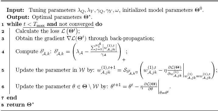
Algorithm 1 provides a summary of the pseudocode for the parameter estimation in our proposed model.

Algorithm 1:

Optimization algorithm for our proposed SIDNN with misrepresentation.

Algorithm 1: Long description

An algorithm for optimizing parameters in a neural network model. The process starts with initialized tuning parameters and model parameters. The algorithm iterates while the maximum iterations are not reached and convergence is not achieved. In each iteration, the loss is calculated through back-propagation, and the gradient is obtained. The algorithm computes a delta value for parameters in set W and updates these parameters using a stochastic gradient descent method. Other parameters are updated similarly. The iteration continues until the stopping criteria are met, and the optimal parameters are returned.

3.6. Summary

To help guide the reader, we briefly summarize the key stages of our methodological framework and the rationale for the penalty structures introduced. In Section 2, we presented a linear model that accounts for unidirectional misrepresentation. To handle high-dimensional covariates, we imposed $\ell_1$ penalties on the coefficients in both the mean and prevalence components, enabling variable selection and mitigating overfitting. Recognizing the limitations of the linear framework, particularly its vulnerability to misspecification bias when the true data-generating process is nonlinear, we introduced a deep learning approach in this section. Within this neural network architecture, standard $L_1$ penalties are insufficient for feature selection because each input connects to multiple hidden units. We therefore adopted group-based penalties that treat all weights from a single input as a group, allowing for feature-level sparsity. Building on this, we proposed a novel $L_1$-gMCP penalty that combines group MCP with LASSO regularization, achieving feature selection with reduced estimation bias. A proximal gradient algorithm is developed for efficient optimization.

4.1. Setting

The data-generating process follows a common configuration across both simulations. The sample size is $N=10,000$ with covariate dimension $p=100$. The covariate vector $\boldsymbol{x}_i=(x_{i1},\ldots, x_{ip})^\top$ is generated from a Gaussian copula, where the element of the covariance matrix $ \boldsymbol{\Sigma} $ is defined as $ \Sigma_{jk} = 0.5^{|j-k|} $ for $ 1 \leq j, k \leq p $. The reported status $v_i^{\ast}$ is generated from $\operatorname{Bernoulli}(0.2)$. The response variable $y_i$ is generated from a normal distribution with mean $\mu_i= -3 + 1.5\exp(x_{i1}) - 1.5 (2 x_{i2} - 1)^2 + 2\sin(2 \pi x_{i3} x_{i4}) - 2\cos(2 \pi x_{i5} x_{i6}) + 3v_i$ and standard deviation $\sigma=1$. The key difference between the two simulations lies in the generation of the true status $v_i$:

• • Simulation 1 (with misrepresentation): For individuals with reported status $v_i^{\ast}=1$, the true status $v_i=1$. For those with $v_i^{\ast}=0$, $v_i$ is generated from Bernoulli($q_i$), where $\operatorname{logit}(q_i) = -3 + \exp(x_{i3}) - 2 (2 x_{i4} - 1)^2 + 3\sin(2 \pi x_{i5} x_{i6}) + 3\cos(2 \pi x_{i7} x_{i8})$. Under this setting, the true misrepresentation rate among the subgroup with $v_i^{\ast}=0$ is 0.472.

• • Simulation 2 (without misrepresentation): We enforce $v_i=v_i^{\ast}$, ensuring no discrepancy between reported and true statuses. The true misrepresentation rate is zero.

We compare five models (M1–M5) across 100 replications for each simulation. In each replication, the data are randomly split into training, validation, and test sets in a 6:2:2 ratio. All models are trained on the training set, with tuning parameters selected using the validation set, and predictive performance is assessed on the test set. The neural network architectures in M3, M4, and M5 consist of four hidden layers with 128, 64, 32, and 32 neurons, respectively. This configuration is selected based on pilot experiments demonstrating stable performance with reasonable computational cost. A dropout rate of 0.1 is applied to enhance robustness and generalization. The Swish activation function, $f(x)=x/(1+e^{-x})$, is used for its ability to capture complex nonlinear patterns while mitigating vanishing-gradient issues. The anchor parameter $\varepsilon$ in M4 is set to $10^{-6}$.

Evaluation metrics include mean squared error (MSE), mean absolute error (MAE), $R^2$, area under the curve (AUC), and F1 score. MSE, MAE, and $R^2$ assess prediction accuracy for y; AUC measures the effectiveness in identifying misreported individuals (only applicable in Simulation 1); and F1 score evaluates variable selection performance. Additionally, we introduce the predicted prevalence of misrepresentation ($\bar{q}$), defined as the average predicted probability of misreporting among individuals with $v_i^{\ast}=0$ in the test set. To save space in the main text, the calculation methods for the corresponding metrics are provided in Appendix B.

4.2. Results

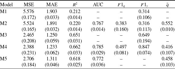
Table 1 reports the mean and standard deviation (in parentheses) of each metric across 100 replications under the misrepresentation scenario. Several key observations can be made from the results. First, neural network-based models (M3–M5) significantly outperform their linear counterparts (M1, M2) across all evaluation dimensions. This aligns with the well-established capacity of neural networks to approximate complex functional forms, as the simulated data contain exponential, quadratic, sine, and cosine transformations. Second, models incorporating misrepresentation correction (M2, M4) consistently outperform their unadjusted analogs (M1, M3) in two critical aspects: prediction accuracy for y and variable selection effectiveness for y. These results underscore the necessity of accounting for misrepresentation when such characteristics are present. Third, despite the conservative regularization anchor ($\varepsilon = 10^{-6}$), the predicted $\bar{q} \approx 0.416$ from M4 suggests a misrepresentation prevalence that aligns fairly closely with the true value of 0.472. This validates the role of the KL term as a stability constraint: when the data signal is sufficiently strong, the regularization does not impede the model’s ability to capture the true underlying distribution. Fourth, the predictive accuracy of M5 for the response variable y is generally inferior to that of both M3 and M4. This shortcoming can be attributed to the element-wise $L_1$ penalty, which fails to completely eliminate irrelevant features. As a result, residual noisy connections remain, ultimately degrading prediction performance. Therefore, it is crucial to combine misrepresentation adjustment with the proposed group-level sparsity penalty in order to fully realize the advantages of our modeling framework.

Table 1.

Comparison results of several candidate models in Simulation 1.

Table 1 Long description

A table comparing performance metrics of five models. The table has six columns: Model, MSE, MAE, R squared, AUC, F1 score at q, F1 score at y, and q bar. There are five rows corresponding to different models labeled M1 to M5. Each row contains values for the performance metrics. For example, Row 1: Model M1, MSE 5.576 (0.172), MAE 1.903 (0.033), R squared 0.212 (0.014), AUC not provided, F1 score at q 0.314 (0.106), F1 score at y not provided, q bar not provided.

Table 2.

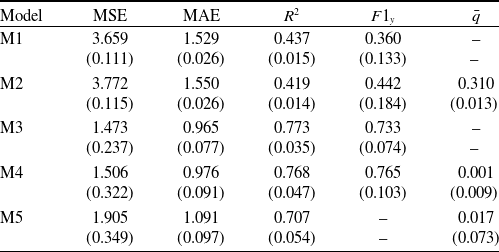
Comparison results of several candidate models in Simulation 2.

Table 2 Long description

A table comparing performance metrics of five models in Simulation 2. The table has five rows and six columns, including headers. The columns are labeled Model, MSE, MAE, R^2, F1_y, and q̅. Each row represents a different model (M1 to M5) with corresponding values for each metric. Row 1: Model M1, MSE 3.659 (0.111), MAE 1.529 (0.026), R^2 0.437 (0.015), F1_y 0.360 (0.133). Row 2: Model M2, MSE 3.772 (0.115), MAE 1.550 (0.026), R^2 0.419 (0.014), F1_y 0.442 (0.184), q̅ 0.310 (0.013). Row 3: Model M3, MSE 1.473 (0.237), MAE 0.965 (0.077), R^2 0.773 (0.035), F1_y 0.733 (0.074). Row 4: Model M4, MSE 1.506 (0.322), MAE 0.976 (0.091), R^2 0.768 (0.047), F1_y 0.765 (0.103), q̅ 0.001 (0.009). Row 5: Model M5, MSE 1.905 (0.349), MAE 1.091 (0.097), R^2 0.707 (0.054), F1_y 0.017 (0.073).

Table 2 presents the comparative results under the no misrepresentation scenario. We focus on three performance criteria: prediction accuracy for y, variable selection effectiveness for y, and the influence of KL divergence regularization in M4. First, neural network-based models continue to demonstrate substantially better predictive performance than their linear counterparts, as anticipated given the nonlinear data-generating process. Second, M3 can be considered the most appropriate baseline in this scenario. Our proposed M4 achieves nearly identical performance to M3 in terms of both prediction accuracy and variable selection, indicating that the misrepresentation adjustment mechanism does not introduce spurious biases when no misrepresentation exists. Third, M4 demonstrates remarkable precision in estimating the absence of misrepresentation, with predicted $\bar{q} \approx 0.001$ that closely aligns with the ground truth of zero. This validates the role of the KL divergence term in correctly penalizing spurious misrepresentation signals. In contrast, M2 again overestimates q, reflecting its limitations in discerning true reporting behavior when the relationship between response and explanatory variables is complex. Fourth, M5 again underperforms M4 in terms of predictive accuracy for y. This further emphasizes the critical role of the structured $L_1$-gMCP penalty in enhancing model effectiveness in this context.

Table 3.

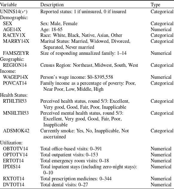
Summary of selected explanatory variables.

Table 3 Long description

A table summarizing selected explanatory variables with their descriptions and types. The table has 22 rows and 3 columns. Column headers are Variable, Description, and Type. Row 1: UNINS14, Reported status: 1 if uninsured, 0 if insured, Categorical. Row 2: SEX, Sex: Male, Female, Categorical. Row 3: AGE14X, Age: 18-65, Numerical. Row 4: RACEV1X, Race: White, Black, Native, Asian, Other, Categorical. Row 5: MARRY14X, Marital Status: Married, Widowed, Divorced, Separated, Never married, Categorical. Row 6: FAMSZEYR, Size of responding annualized family: 1-14, Numerical. Row 7: REGION14, Census Region: Northeast, Midwest, South, West, Categorical. Row 8: WAGEP14X, Person's wage income: $0-$395,558, Numerical. Row 9: POVCAT14, Family income as a percentage of poverty: Poor, Near Poor, Low, Middle, High, Categorical. Row 10: RTHLTH53, Perceived health status, round 5/3: Excellent, Very good, Good, Fair, Poor, Inapplicable, Categorical. Row 11: MNHLTH53, Perceived mental health status, round 5/3: Excellent, Very good, Good, Fair, Poor, Inapplicable, Categorical. Row 12: ADSMOK42, Currently smoke: Yes, No, Inapplicable, Not ascertained, Categorical. Row 13: OBTOTV14, Total office-based visits: 0-391, Numerical. Row 14: OPTOTV14, Total outpatient visits: 0-153, Numerical. Row 15: ERTOT14, Total emergency room visits: 0-18, Numerical. Row 16: IPDIS14, Total inpatient stays (including zero-night stays): 0-10, Numerical. Row 17: RXTOT14, Total prescription medicines: 0-344, Numerical. Row 18: DVTOT14, Total dental visits: 0-27, Numerical.

5.1. Data description

In this study, we use the 2014 consolidated data from the Medical Expenditure Panel Survey (MEPS), as previously examined by Akakpo et al. (Reference Akakpo, Xia and Polansky2019) to investigate the presence of misrepresentation in insurance status. The dataset is available from the MEPS website https://meps.ahrq.gov/. A potential incentive for reporting inaccurate insurance status arises from the 2014 Affordable Care Act reforms imposing a tax penalty for lacking health insurance. Social desirability and financial concerns may drive MEPS respondents to misrepresent their insurance status.

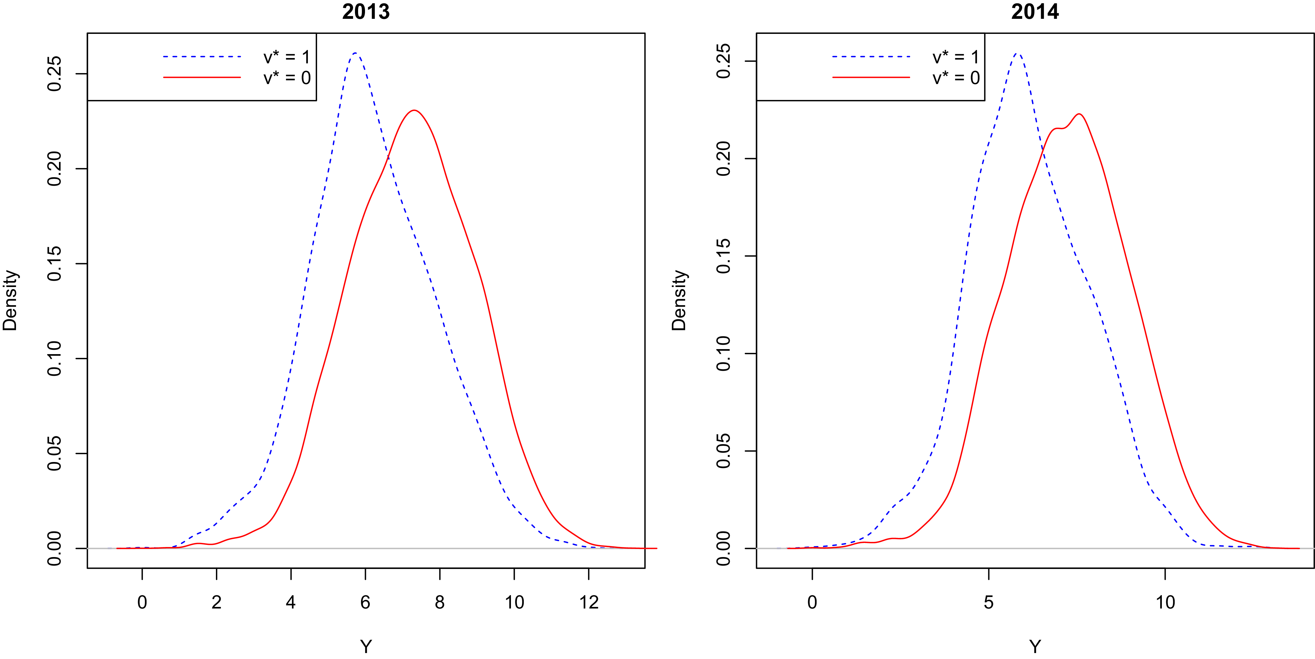
The raw dataset contains information on 34,875 individuals. For our analysis, we retain individuals aged 18–65 years with positive health expenditures. Additionally, we exclude individuals whose health status and mental health status fall into rare categories. After processing, the dataset includes 15,865 records. Selected predictors are displayed in Table 3. Some categorical variables have multiple levels (e.g., race, marital status, and health status), which expand the dimensionality of the explanatory variables to 39 dimensions. The response variable of interest is the log-transformed total health care expenditure. Density plots of the response variable, categorized by reported insurance status, are presented in Figure 3. We denote $v_i^{\ast}=1$ if the respondent reports being uninsured, and $v_i^{\ast}=0$ otherwise. A distinct bimodal distribution is evident for the reported insured group in 2014, whereas the corresponding distribution in 2013 lacks this clarity. This temporal difference provides preliminary evidence consistent with systematic misrepresentation of insurance status specifically in 2014.

In our analysis, we randomly split the data into a training, validation, and test set as seen in Table 4. The training set is used to develop the model, the validation set is used to select tuning parameters, and predictive performance is assessed on the test set. In addition to our proposed DNN model with misrepresentation and the $L_1$-gMCP penalty (M4), the other four candidate models (M1, M2, M3, M5) are identical to those used in the simulation studies. All numerical explanatory variables are scaled before they are fed into the model.

5.2. Model fitting

We provide a brief overview of the architectures used for the three deep learning models. To ensure comparability, M3, M4, and M5 adopt the same underlying network architecture. Specifically, each network is a feedforward neural network with four hidden layers, featuring 96, 64, 32, and 32 neurons, respectively. All hidden layers use the Swish activation function (as previously defined). To prevent overfitting, a dropout rate of 0.1 is applied to the output of each hidden layer.

Table 4.

Data partitioning.

Table 4 Long description

A table with four rows and four columns detailing the partitioning of data into training, validation, and test sets. The columns are labeled Set, Symbol, Number of individuals, and Proportion (percent). The rows are labeled as follows: Training with symbol T subscript r, 9,519 individuals, and 60 percent; Validation with symbol V subscript a, 3,173 individuals, and 20 percent; Test with symbol T subscript e, 3,173 individuals, and 20 percent.

Figure 3.

Density plots for log-transformed positive total medical expenditure categorized by reported insurance status.

Table 5.

Variable selection under four models.

Table 5 Long description

A table comparing variable selection across four models. The table has 42 rows and 9 columns. The columns are labeled Q M1, Q M2, Q M3, Q M4, Y M1, Y M2, Y M3, and Y M4. The rows are labeled with different variables such as SEX: Female, AGE14X, RACEV1X: Black, RACEV1X: Native, RACEV1X: Asian, RACEV1X: Other, MARRY14X: Widowed, MARRY14X: Divorced, MARRY14X: Separated, MARRY14X: Never married, FAMSZEYR, REGION14: Midwest, REGION14: South, REGION14: West, WAGEP14X, POVCAT14: Near Poor, POVCAT14: Low, POVCAT14: Middle, POVCAT14: High, RTHLTH53: Excellent, RTHLTH53: Very good, RTHLTH53: Good, RTHLTH53: Fair, RTHLTH53: Poor, MNHLTH53: Excellent, MNHLTH53: Very good, MNHLTH53: Good, MNHLTH53: Fair, MNHLTH53: Poor, ADSMOK42: Inapplicable, ADSMOK42: Yes, ADSMOK42: No, OBTOTV14, OPTOTV14, ERTOT14, IPDIS14, RXTOT14, DVTOT14. Each cell contains a checkmark indicating the presence of the variable in the respective model.

The hyperparameter tuning for these three deep learning models follows a rigorous protocol. For the MCP penalty’s concavity parameter $\gamma$, we explore values within the set {3, 6, 9, 12}. Other critical regularization hyperparameters (i.e., $\lambda,\omega$) are determined through an exhaustive grid search, with optimal values selected from predefined candidate grids based on minimizing the validation MSE. The learning rate $\eta$ is fixed at 0.001 with a batch size of 512, and $\varepsilon$ is set to $10^{-6}$. To mitigate overfitting, an early stopping mechanism is employed. Models are trained for a sufficient number of epochs, with final model selection based on the epoch that achieves the minimum MSE on the validation set.

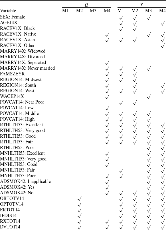
Since M5 does not perform feature-level variable selection, we only present the variable selection results for models M1 through M4 in Table 5. Notably, the four models consistently identify healthcare service utilization as selected predictors of expenditure (y). This finding aligns well with established health economic theory, where increased healthcare utilization naturally leads to higher medical expenditures. In terms of predicting the prevalence of misrepresentation (q), we observe that M4 incorporates a more comprehensive set of explanatory variables compared to M2. Importantly, both models share two common active predictors for q: RXTOT14 and DVTOT14.

Figure 4.

SHAP summary plots of the most important variables considered in $\text{NN}_Y$ and $\text{NN}_Q$ under M4.

Algorithm 1: Long description

An algorithm for optimizing parameters in a neural network model. The process starts with initialized tuning parameters and model parameters. The algorithm iterates while the maximum iterations are not reached and convergence is not achieved. In each iteration, the loss is calculated through back-propagation, and the gradient is obtained. The algorithm computes a delta value for parameters in set W and updates these parameters using a stochastic gradient descent method. Other parameters are updated similarly. The iteration continues until the stopping criteria are met, and the optimal parameters are returned.

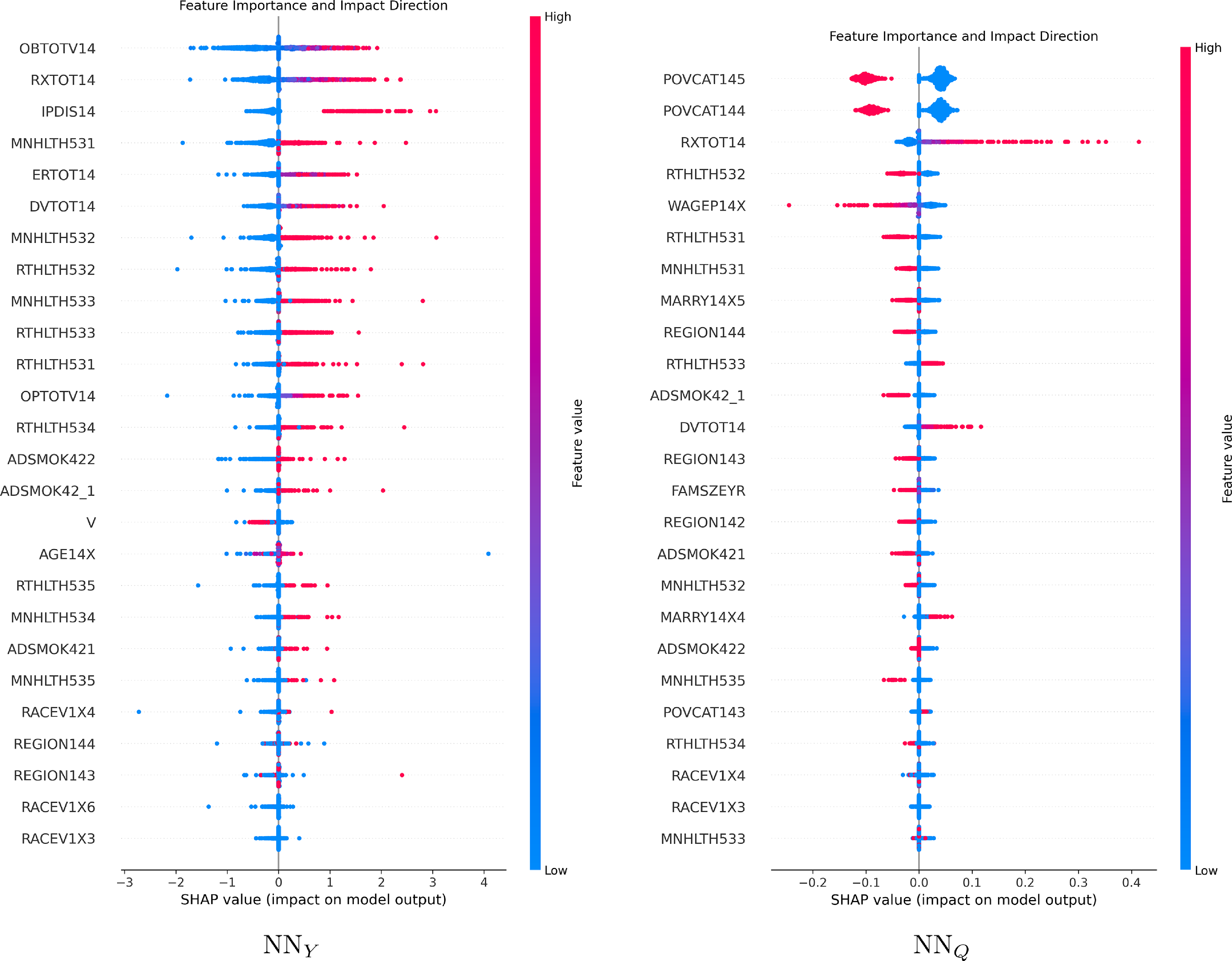
To gain deeper insights into the decision-making mechanisms and interpret variable importance in M4, this study employs SHAP (SHapley Additive exPlanations) (Lundberg and Lee, Reference Lundberg and Lee2017). This cutting-edge method in explainable AI has gained significant recognition in recent years. The corresponding plots are displayed in Figure 4. In the summary plot, the vertical axis represents features ranked by their importance, while the horizontal axis quantifies each feature’s contribution to model outputs through SHAP values. Each point corresponds to an observation, with the color intensity indicating feature values (red for high, blue for low). Positive SHAP values indicate that the feature increases the predicted outcome, while negative values suggest a decreasing effect. Our core model, M4, addresses misrepresentation through two specialized sub-networks ($\text{NN}_Y$ and $\text{NN}_Q$). The SHAP analysis reveals distinct patterns learned by each sub-network, providing valuable interpretability into their respective decision-making processes. From the left panel, we can observe that healthcare utilization variables (e.g., OBTOTV14, RXTOT14, IPDIS14) are the most influential factors in the prediction, all demonstrating positive effects on medical costs. Notably, insurance status also plays a significant role: when the status is uninsured, it substantially lowers the baseline cost prediction. On the right panel, we find that socioeconomic status variables, such as POVCAT145 (high-income households), POVCAT144 (middle-income households), and WAGEP14X (wage income), are key determinants in identifying potential misrepresentation. Higher values of these features correspond to increasingly negative SHAP values, indicating that individuals with higher income levels exhibit lower predicted probabilities of potential misrepresentation. Conversely, healthcare utilization variables such as RXTOT14 (total prescription medicines) show positive associations, systematically increasing the predicted likelihood of misrepresentation.

5.3. Predictive performance

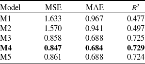
To assess the predictive performance of the five candidate models, we employ multiple diagnostic approaches. First, we evaluate and compare the performance of the five models using multiple metrics, including MSE, MAE, and $R^2$. The detailed results are presented in Table 6. Consistent with theoretical expectations, the three neural network-based models demonstrate superior predictive accuracy compared to their linear counterparts. This empirical finding underscores the necessity of employing nonlinear, complex modeling frameworks to capture the underlying patterns in this dataset. Notably, the performance gains observed when transitioning from M1 to M2 and from M3 to M4 suggest the presence of misreported cases within the data. This inference aligns with the conclusions drawn in Akakpo et al. (Reference Akakpo, Xia and Polansky2019), further reinforcing the validity of our methodological approach. 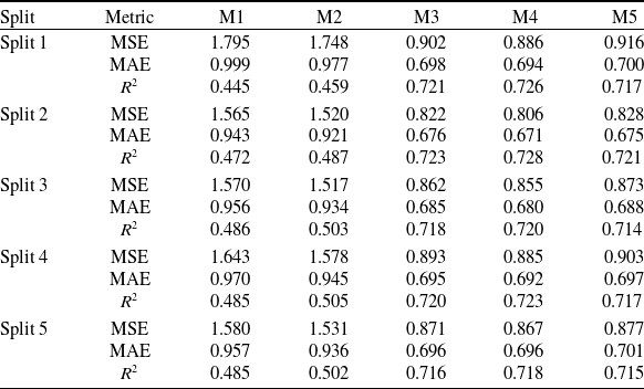The comparison of M4 and M5 demonstrates the effectiveness of incorporating the $L_1$-gMCP compared to the standard $L_1$ penalty. To ensure the robustness of the comparison and mitigate the impact of data partitioning, we repeated the experiments using five distinct random splits. The aggregated results across all splits are reported in Appendix C. Across all splits, M4 consistently outperforms the other candidate models in terms of MSE, MAE, and $R^2$, with the same direction and similar magnitude of improvement. Notably, in Split 5, M4’s marginal MAE advantage over M3 is obscured by rounding in the tabulated values. Collectively, these results support the robustness of the observed performance gain across data splits.

Table 6.

Comparison of criteria across five models.

Table 6 Long description

A table comparing predictive performance metrics across five models. The table has five rows and four columns. The columns are labeled Model, MSE, MAE, and R squared. The rows are labeled M1, M2, M3, M4, and M5. Row 1: Model, M1; MSE, 1.633; MAE, 0.967; R squared, 0.477. Row 2: Model, M2; MSE, 1.570; MAE, 0.941; R squared, 0.497. Row 3: Model, M3; MSE, 0.858; MAE, 0.688; R squared, 0.725. Row 4: Model, M4; MSE, 0.847; MAE, 0.684; R squared, 0.729. Row 5: Model, M5; MSE, 0.861; MAE, 0.688; R squared, 0.724.

Table 7.

The Gini indices of health expenditures for five models on the test data.

Table 7 Long description

A table comparing Gini indices of health expenditures for five models. The table has six rows and seven columns, including a row for the base model and columns for competing models and minimax values. Row 1: Base model M1, M2 3.554, M3 6.732, M4 6.805, M5 6.803, Minimax 6.805. Row 2: Base model M2, M1 -2.718, M2 0.000, M3 6.437, M4 6.517, M5 6.504, Minimax 6.517. Row 3: Base model M3, M1 -0.315, M2 -0.313, M3 0.000, M4 1.086, M5 0.735, Minimax 1.086. Row 4: Base model M4, M1 -0.166, M2 -0.164, M3 0.314, M4 0.000, M5 0.446, Minimax 0.446. Row 5: Base model M5, M1 -0.672, M2 -0.649, M3 0.865, M4 1.163, M5 0.000, Minimax 1.163.

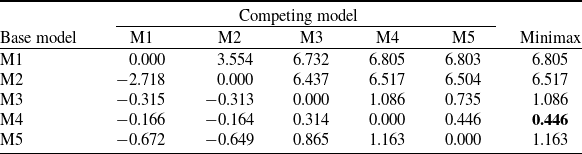
To evaluate the risk-differentiation ability of models predicting expenditures, we utilize the Gini indices, a well-established metric derived from Lorenz curve analysis. As demonstrated in Frees et al. (Reference Frees, Meyers and Cummings2011, Reference Frees, Meyers and Cummings2014), Gini indices provide a robust measure of a model’s ability to discriminate risk by quantifying the alignment between predicted and actual loss distributions. Our comparative analysis proceeds as follows: for each candidate model (M1–M5), we treat its predicted losses as the base distribution and compute Gini indices against competing predictions from alternative models. The complete matrix of pairwise Gini comparisons is presented in Table 7. To objectively identify the optimal model, we implement a minimax selection strategy: for each model, we determine its maximum Gini index across all possible competing model comparisons; we then select the model exhibiting the smallest maximum Gini value. This conservative approach identifies the most stable performer – the model least sensitive to variations in ranking basis. As Table 7 demonstrates, M4 emerges as superior with the lowest maximum Gini index (0.446) among all candidates.

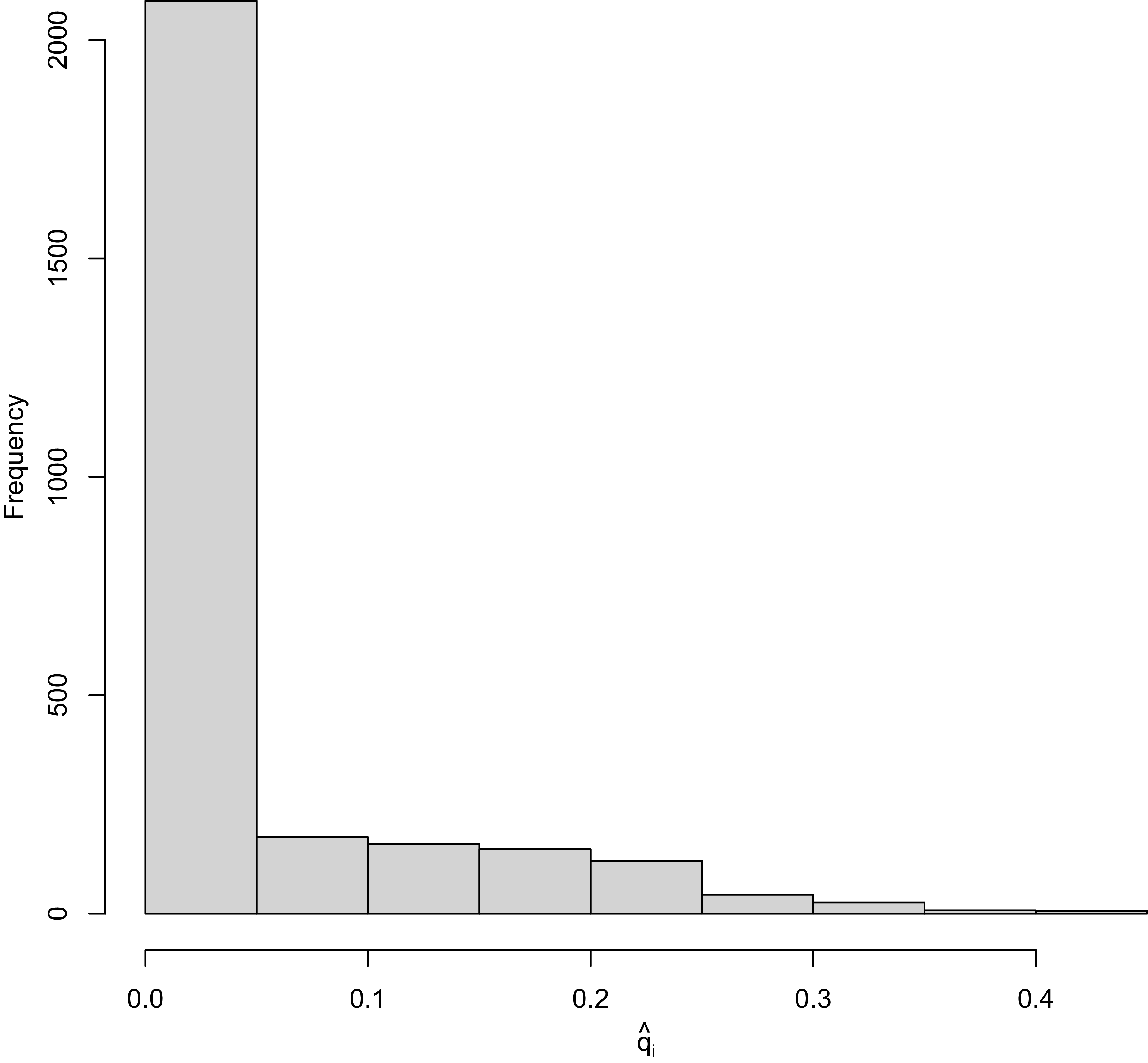
Finally, Figure 5 presents a histogram of the predicted misrepresentation probabilities $\widehat{q}_i$ from M4 for individuals with reported insurance status $v_i^* =0$. The distribution is highly skewed toward zero: the majority of individuals have $\widehat{q}_i$ very close to 0, indicating that the model classifies most respondents as truthful. A small proportion of individuals exhibit elevated $\widehat{q}_i$ values, suggesting that the model identifies a subset of potentially misreporting individuals based on their covariate patterns. The average predicted prevalence of misrepresentation among respondents with $v_i^* =0$ is $\bar{q} \approx 4.3\%$. It is noteworthy that our estimate of misrepresentation probability is substantially lower than the estimate of 18% reported by Akakpo et al. (Reference Akakpo, Xia and Polansky2019). One possible explanation is the difference in model specification: our method accommodates nonlinear covariate effects, whereas the comparison model uses a more restrictive parametric structure.

Figure 5.

Histogram of the predicted misrepresentation probabilities $\widehat{q}_i$ from M4 for individuals with reported insurance status $v_i^* =0$.

5.4. Summary

Although the application focuses on health care expenditures, the proposed framework offers broader implications for the insurance industry. First, compared with conventional linear models, the deep learning framework achieves a substantial improvement in claim severity prediction accuracy, capturing complex nonlinearities that traditional approaches cannot accommodate. Second, the predicted misrepresentation probabilities $q_i$ serve primarily as a screening tool to prioritize policies for external verification and manual underwriting review. Only after such validation can these estimates inform adjustments to the insured’s risk profile. Consequently, rather than relying solely on potentially misstated self-reported information, this process mitigates adverse selection and supports actuarially fair pricing within a robust governance framework. Third, the KL divergence regularization embeds a “presumption of honesty” into the learning process, flagging misrepresentation only when strongly supported by the data. This design reduces the operational cost and reputational risk associated with investigating wrongly suspected policyholders, while directing audit and anti-fraud resources toward higher-risk cases. Fourth, the sparse structure induced by the $L_1$-gMCP penalty identifies the most influential drivers of claim severity. This enhances operational efficiency by streamlining data collection, simplifying underwriting workflows, and ensuring that risk assessment focuses on the variables with the greatest predictive value.