


1. Introduction
Satellite imagery provides a full view of sea-ice motion in the polar region every day. Because of this unprecedented capability, it has frequently been used to study polar sea-ice motion and has made an important contribution to better understanding it. Reference Emery, Fowler, Hawkins and PrellerEmery and others (1991) used sequential satellite images obtained from the Advanced Very High Resolution Radiometer (AVHRR) to determine ice motion through ice-feature tracking. Using different approaches, Reference Kwok, Schweiger, Rothrock, Pang and KottmeierKwok and others (1998) and Reference Liu and CavalieriLiu and Cavalieri (1998) demonstrated that sequential imagery from the Defense Meteorological Satellite Program (DMSP) Special Sensor Microwave/Imager (SSM/I) 85 GHz could provide ice-motion observations, where Kwok and others based their method on cross-correlation, and Liu and Cavalieri on wavelet transform. Reference Liu, Zhao and LiuLiu and others (1998) reported unexpected success in using the NASA scatterometer (NSCAT) to measure sea-ice motion, even though NSCAT was not designed for this purpose. However, satellite imagery has limitations too. For example, AVHRR images are obscured by cloud cover and seasonally varying low light level. Radar systems such as European Remote-sensing Satellite 1 (ERS-1) synthetic aperture radar (SAR) and RADARSAT are independent of weather conditions and should provide good estimates of ice drift (Reference Kwok, Rothrock, Stern and CunninghamKwok and others, 1995), but less than daily coverage makes them unsuitable for some applications. SSM/I 85 GHz radiance data have atmospheric emission effect at this frequency, as well as surface effects that may give a false indication of ice drift. NSCAT is an active sensor and is not affected by cloud cover, but its resolution is relatively low. So, the combined use of several satellite imageries is obviously important in order to obtain more accurate and complete ice-motion data. Reference Liu, Zhao and WuLiu and others (1999) reported that sea-ice motion derived from wavelet analysis of SSM/I and NSCAT for November and December 1996 gave good quantitative agreement with the ice motion derived from buoy data, and ice-motion values from these two satellite datasets were compatible and complemented each other when SSM/I data had cloud or surface effects. Therefore, three sea-ice-motion daily results from SSM/I, NSCAT and buoy data could be merged by data-fusion techniques to produce a composite map with more complete coverage of sea-ice motion than a sea-ice motion map from a single data source. It was also found that sea-ice flow streamlines constructed from the merged sea-ice motion data were highly correlated with the surface pressure contours, implying that sea ice was dominated by wind forcing.
This paper is focused on quantifying the wind effects on Arctic sea-ice motion using our merged sea-ice motion data from sea-ice tracking results of SSM/I, NSCAT and buoy data for the period October 1996−March 1997. Reference Thorndike and ColonyThorndike and Colony (1982) studied the response of Arctic sea-ice motion to geostrophic winds using buoy datasets collected during the First Global Atmospheric Research Program Experiment in 1979 and 1980, and the Arctic Ice Dynamics Joint Experiment in 1975−76. They found that only about half of the long-term (several-month) average ice motion is directly related to the geostrophic wind, the other half being due to the mean ocean circulation. Compared to the existing array of ocean buoys, the merged Arctic sea-ice motion data provide improved spatial coverage. It is therefore worth taking a fresh look at the wind effects on Arctic sea-ice motion. Also, instead of estimating a direct relationship between the ice velocity, the geostrophic wind and the mean ocean current, principal-component analysis (PCA) is applied to merged sea-ice-motion and pressure-field data for the period October 1996−March 1997 to derive correlation information about wind and sea-ice motion patterns.
In section 2 we describe a two-dimensional Gaussian wavelet transform and present the wavelet analysis for ice-feature tracking and sea-ice motion from SSM/I and NSCATdata, along with some discussion of algorithms and techniques. In section 3 we describe the PCA for merged sea-ice motion data and the pressure field. In section 4 we discuss the results and applications of satellite-derived sea-ice motion and the extension of the ice-tracking procedure to be used with QuikSCAT.
2. Wavelet Analysis of SSM/I and Nsgat Imageries
An ice-tracking procedure based on wavelet transform has been developed at NASA Goddard Space Flight Center, where it has been used for the past few years. Basically wavelet transforms are analogous to a Fourier transform but are localized in both frequency and time (e.g. Reference Combes, Grossmann and TchamitchianCombes and others, 1989). A two-dimensional wavelet transform is a highly efficient band-pass filter. It has been used in various applications in physical oceanography (see, e.g., Reference Liu, Peng and WeingartnerLiu and others, 1994, Reference Liu, Martin and Kwok1997a, Reference Liu, Peng and Changb, Reference Liu, Zhao and Liu1998, Reference Liu, Zhao and Wu1999; Reference Peng, Liu, Chapron and Mollo-ChristensenPeng and others, 1995; Reference Liu and CavalieriLiu and Cavalieri, 1998).
In general, the two-dimensional continuous wavelet transform  of a function
 , where
 is expressed in terms of the complex valued wavelet function
 as follows:

where the wavelet function is dilated by the factor a and shifted by the vector  . The function
 is the basic wavelet (Reference Combes, Grossmann and TchamitchianCombes and others, 1989). The superscript * indicates complex conjugate. Two frequently used wavelet functions are the Morlet wavelet, a Gaussian modulated sine and cosine wave packet, and the Mexican hat, the second derivative of a Gaussian function. In this study, we use the Mexican hat that can be expressed as follows:

Since convolution is commutative with respect to differentiation, the resulting wavelet transform is the Laplacian of a Gaussian smoothed function. Thus, zeroes correspond to the inflection points of the original function. The contours of zero crossing indicate the edges in the pattern of the input function.
Now we outline our ice-tracking procedure based on wavelet transform. We refer readers to Reference Liu and CavalieriLiu and Cavalieri (1998) and Reference Liu, Zhao and WuLiu and others (1999) for detailed description of the procedure. Daily satellite images (in this case, SSM/I 85 GHz and NSCAT 14 GHz) of the entire Arctic region are first constructed and interpolated to fit the numerical grid, with land masked out. Then the wavelet transform defined by Equations (1) and (2) is applied to the interpolated satellite images at various scales to separate various ice textures or features. In this case, for NSCAT images scale a = 1.0, 1.21 and 1.414, and for SSM/I images a = 2.0, 2.42 and 2.428, since pixel spacing for interpolated NSCAT images is twice as large as for interpolated SSM/I images. The choice of the scales for wavelet transform depends on the physical scales of the ice signatures (brightness temperature for SSM/I and backscatter/roughness for NSCAT) to be extracted. The effect of this wavelet transform is a band-pass filter with a threshold for feature detection. Then template matching is performed to determine ice velocities. Figure 1a shows an Arctic ice-motion map in a grid of 100 km × 100 km derived from wavelet analysis of SSM/I on 18 December 1996, and Figure 1b shows an Arctic ice-motion map derived from wavelet analysis of NSCAT data on the same day. The Arctic buoy data are obtained from the International Arctic Buoy Program (IABP) datasets via the Web (http://iabp.apl.washington.edu/data.html). Notice that the ice circulation has been clearly derived and agrees with the ice velocities derived from buoy data. Also, the flow patterns in these two images are extremely similar and complement each other well, where the areas with no ice velocities in one motion map are not empty areas in another map. The areas with no ice velocities indicate failure of the template to identify displacement within a threshold value. Reference Liu, Zhao and WuLiu and others (1999) compared sea-ice motion derived from wavelet analysis of SSM/I and NSCAT data as described above with the ice motion derived from the buoy data for November and December 1996 and found good quantitative agreement. They also found that the flow patterns were very similar and complemented each other well. Therefore, the results from SSM/I, NSCATand buoy data could be merged to form composite maps with more complete coverage of sea-ice motion by data-fusion techniques, and ice-flow streamlines constructed from merged ice motion were highly correlated with surface air-pressure contours. Figure 2 shows a merged ice-motion map on 18 December 1999 from ice-motion results derived from SSM/I and NSCATdata and from buoy data. It is obvious from Figures 1 and 2 that the merged ice-motion map provides more complete coverage of sea-ice motion than the ice-motion map from only one data source. We use the merged sea-ice motion data in the next section to quantify wind effects on sea-ice motion.
Arctic sea-ice motion maps in a grid of 100 km × 100 km derived from wavelet analysis of (a) ssm/i data and (b) nsgat data, on 18 december 1996. white arrows are ice velocities derived from ssm/i or nscat data; black arrows are ice velocities derived from buoy data.

Merged arctic sea-tee motion map from ssm/i, nscatand buoy data.

3. PCA of Ice Drift and Pressure
PCA as used by meteorologists and oceanographers is a tool for analyzing the spatial or temporal variability of physical fields and has long been used in the research community. Its attraction as a diagnostic tool is its ability to reduce the many-dimensional complexity of the observed fields to relatively easily visualized low-dimensional representations using eigenvectors (empirical orthogonal functions (EOFs)) generated from the given dataset (Reference PreisendorferPreisendorfer, 1988). Its mathematical essential is to find a set of EOFs to decompose the original centered dataset exactly as a sum of scale products of EOFs and principal components (also called amplitudes), where principal components depend only on time and therefore can be thought of as time series. We refer readers to Reference PreisendorferPreisendorfer (1988) for a detailed treatment of PCA. In the following two subsections, we describe our PCA algorithm for ice-drift and pressure-field data.
3.1. PCA of ice drift
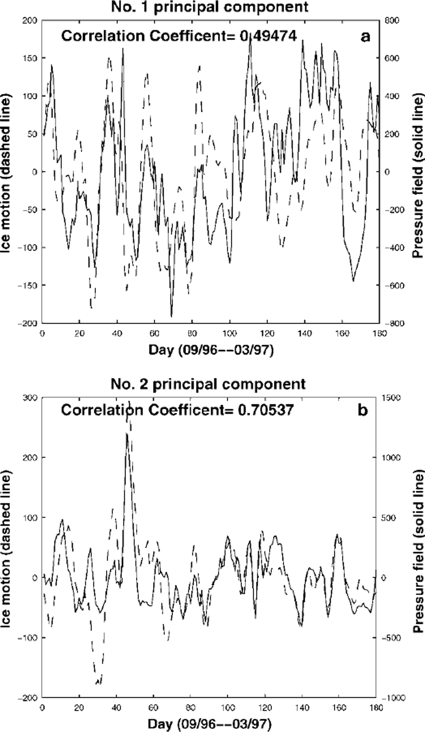
In this subsection we first describe our PCA algorithm for ice-drift data. The ice-drift data used are merged sea-ice motion, as described in the previous section, for the period October 1996−March 1997. Since these data are obtained from the ice-tracking procedure, there are locations in the daily map where no ice-motion information is provided because tracking results do not meet the criteria imposed. To minimize the number of missing data points in the PCA, we first determine the area where we perform PCA by including only those locations where non-zero ice motion is registered by our tracking procedure for at least half of the study period. Then we construct the raw-data array for PCA where each row represents daily ice-drift data at the selected locations, and the row number corresponds to the day number within the period. Since each ice velocity has two components, the U-components of ice velocities are stored in the first half-row and the V-components in the second half-row We can thus take advantage of the simplicity of the PCA for a real-valued scale dataset while studying a vector-valued dataset. However, in interpreting the PCA results, we must take it into account that the first half of each row of the data array corresponds to U-components of ice velocities, and the second half of each row to V-components of ice velocities. Therefore, we can pair eigenvector components that correspond to U-components with those corresponding to V-components so that an eigenvector can be viewed as a set of ice velocities at the observation locations. Figure 3 shows the plots of modes 1 and 2 of the PCA, interpreted in this way, for the period October 1996−March 1997. Mode 1 in Figure 3 is basically transpolar motion, while mode 2 has a variety of motions that include a general circular motion around a center northeast of the North Pole and a motion going out to Greenland and a convergent zone in the Beaufort Sea. Modes 1 and 2 account for 16.2% and 13.2% of variance of the entire dataset, respectively. These percentages of variance are consistent with the results in Reference Wang and IkedaWang and Ikeda (2000) where the modes 1 of the PCAs of sea-level pressure, surface air temperature and sea-ice area account for 16.9%, 14.9% and 40.7% of variance of entire datasets, respectively. The dashed lines in Figure 4 show the principal components of modes 1 and 2 of sea-ice motion. For higher modes, the percentages of variance that they account for decay exponentially.
Modes 1 (a) and 2 (b) of pca of merged sea-iee drift derived from wavelet analysis of ssm/i and nscatdata for the period october 1996−march 1997. the empty spot in the center of the plots is around the north pole.

Principal components of modes 1 (a) and 2 (b) of pca of merged sea-ice drift (dashed line) and of pressure field (solid line) for the period october 1996−march 1997.
3.2. PCA of pressure field
To quantify the wind forcing on sea-ice motion, we apply the PCA to the pressure-field data obtained from the IABP program. The IABP pressure-field data are given in longitude and latitude and have a resolution of 10° × 2°. To find pressure values at pixels of the rectangular coordinate system of sea-ice motion data, the IABP pressure data are first projected to the rectangular coordinate system. After projection, the pressure data points may not locate at the pixel points. For each pixel point in the target area, the four closest pressure data points are found, then four-point bilinear interpolation is used to compute pressure value at the pixel point. The PCA for general real-valued scale datasets is then performed for the interpolated pressure field in the target area. Figure 5 shows contours of modes 1 and 2 of the PCA of the pressure field for the period October 1996−March 1997. The principal components of modes 1 and 2 of the pressure field are shown in Figure 4 as solid lines. The contours of mode 1 in Figure 5 indicate that mode 1 wind motion is basically transpolar, and the contours of mode 2 reveal that the general wind motion is circular around a center near the North Pole. Modes 1 and 2 account for 31.7% and 17.1% of the variance of the entire dataset, respectively. For higher modes, the percentages of variance that they account for show exponential decay.
Contours of modes 1 (a) and 2 (b) of pca of pressure field in the arctic for the period october 1996−march 1997.

3.3. Estimation of wind effects on sea-ice motion
It is clear from Figures 3 and 5 that for modes 1 and 2 of the two PCAs the ice-motion patterns are very similar to the wind patterns. To see this more clearly, Figure 6 shows overlaid modes 1 and 2 of the PCA of pressure-field data and of the PCA of merged sea-ice drift, respectively. The rms of angles between sea-ice motion and pressure contours is 42° and 34° for modes 1 and 2, respectively, which is consistent with the Ekman effects of wind drag for sea-ice drift. For principal components, one can see from Figure 4 that the principal components of modes 1 and 2 from the two PCAs are highly correlated. Actually, the correlation coefficient for principal components of mode 1 from the two PCAs is 0.5 and for principal components of mode 2 is 0.7. Notice that modes 1 and 2 of sea-ice motion data account for 30% of the variance of the entire sea-ice motion dataset, and modes 1 and 2 of the pressure-field data account for 50% of the variance of the entire pressure-field dataset. Therefore, those correlation coefficients indicate that 30% of sea-ice motion is highly correlated with 50% of the pressure field in modes 1 and 2. Thus, wind forcing is clearly a driving force of ice drift. However, modes 3−5 of the PCAs of ice drift and pressure field do not show overall agreement between the wind pattern and the sea-ice motion pattern. The correlation coefficients for principal components of modes 3−5 of the two PCAs are only 0.3, 0.44 and 0.17, respectively. These three modes account for 7.5%, 6.3% and 4.4% of the variance of the entire dataset for ice drift, and 11.9%, 9.8% and 8.4% of the variance of the entire dataset for pressure field, respectively. The poor agreement between the ice-motion pattern and the wind pattern for modes 3−5, and the small correlation coefficients for the principal components of these modes indicate that the wind forcing is not the only driving force for ice drift. For the higher modes, sea-ice motion is also affected by ocean current, bathymetry and coastal boundary and is therefore not highly correlated with the wind field.
Overlaid modes 1 (a) and 2(b) of pca of merged tee-motion data derived from satellite data (vectors) and pcaof pressure-field data (contours) for the period october 1996–march 1997.

4. Discussion
In this paper, a two-dimensional Gaussian wavelet transform is used to derive sea-ice motion in the Arctic from SSM/I and NSCATdata for the fall/winter period October 1996−March 1997. This technique provides improved spatial coverage over the existing array of Arctic Ocean buoys and better temporal resolution than techniques using data from satellite SAR. This new source of ice-motion data offers a potential solution to the problem of inadequate temporal sampling. Reference Liu, Zhao and WuLiu and others (1999) compared sea-ice motion results derived from wavelet analysis of SSM/I and NSCAT for November and December 1996 with the ice drift derived from buoy data. It was found that results from both NSCAT and SSM/I gave good quantitative agreement with ice drift derived from buoy data, and the flow patterns from results of SSM/I and NSCAT were extremely similar, and the two sets of results complemented each other well. Therefore, the ice-motion results from SSM/I, NSCATand buoy data could be merged by data-fusion techniques to form composite maps with more complete coverage of sea-ice motion than the results from a single data source. It was also found that sea-ice flow streamlines constructed from the merged sea-ice motion data were highly correlated with the surface pressure contours, implying that sea-ice motion was dominated by wind forcing. To quantify the wind effects on sea-ice motion, PCA is applied to merged sea-ice motion data and to pressure-field data in this paper. It is found that 30% of sea-ice motion is highly correlated with 50% of the pressure field in modes 1 and 2. The rms of angles between sea-ice motion and pressure contours is 42° and 34° for modes 1 and 2, respectively, which is consistent with the Ekman effects of wind drag for sea-ice drift. For higher modes, sea-ice motion is probably also affected by ocean current, bathymetry and coastal boundary and therefore is not highly correlated with the wind field. We shall continue research in this direction.
QuikSCAT, a "quick recovery" mission to fill the gap created by the loss of data from NSCATwhen the ADEOS-1 satellite lost power in June 1997, was launched on 19 June 1999. It will continue to add to the important ocean-wind dataset begun by NSCAT in September 1996. QuikSCAT has 25 km resolution with 5 km resolution from enhanced processing. The finer resolution will reduce the uncertainty of the ice-motion product that inherits from satellite data, and therefore may improve its accuracy. For a discussion on error sources of ice-tracking results, we refer readers to Reference Kwok, Schweiger, Rothrock, Pang and KottmeierKwok and others (1998), Reference Liu, Zhao and WuLiu and others (1999) and Reference Zhao, Liu and GeigerZhao and others (2000). The wavelet-analysis algorithms for daily sea-ice motion have been extended to use QuikSCATdata in the automated near-real-time processing. The limitations of QuikSCAT backscatter data for sea-ice motion during the summer months have been investigated by optimizing the scales chosen in the wavelet transform. We will report the ice-motion results from wavelet analysis of QuikSCATdata in the near future. Because of good quantitative agreement between sea-ice motion values from wavelet analysis of SSM/I and NSCAT data and from buoy data, the daily sea-ice motion map can also be used to improve our current knowledge of sea-ice dynamics and process through data assimilation of an ocean-ice numerical model.



