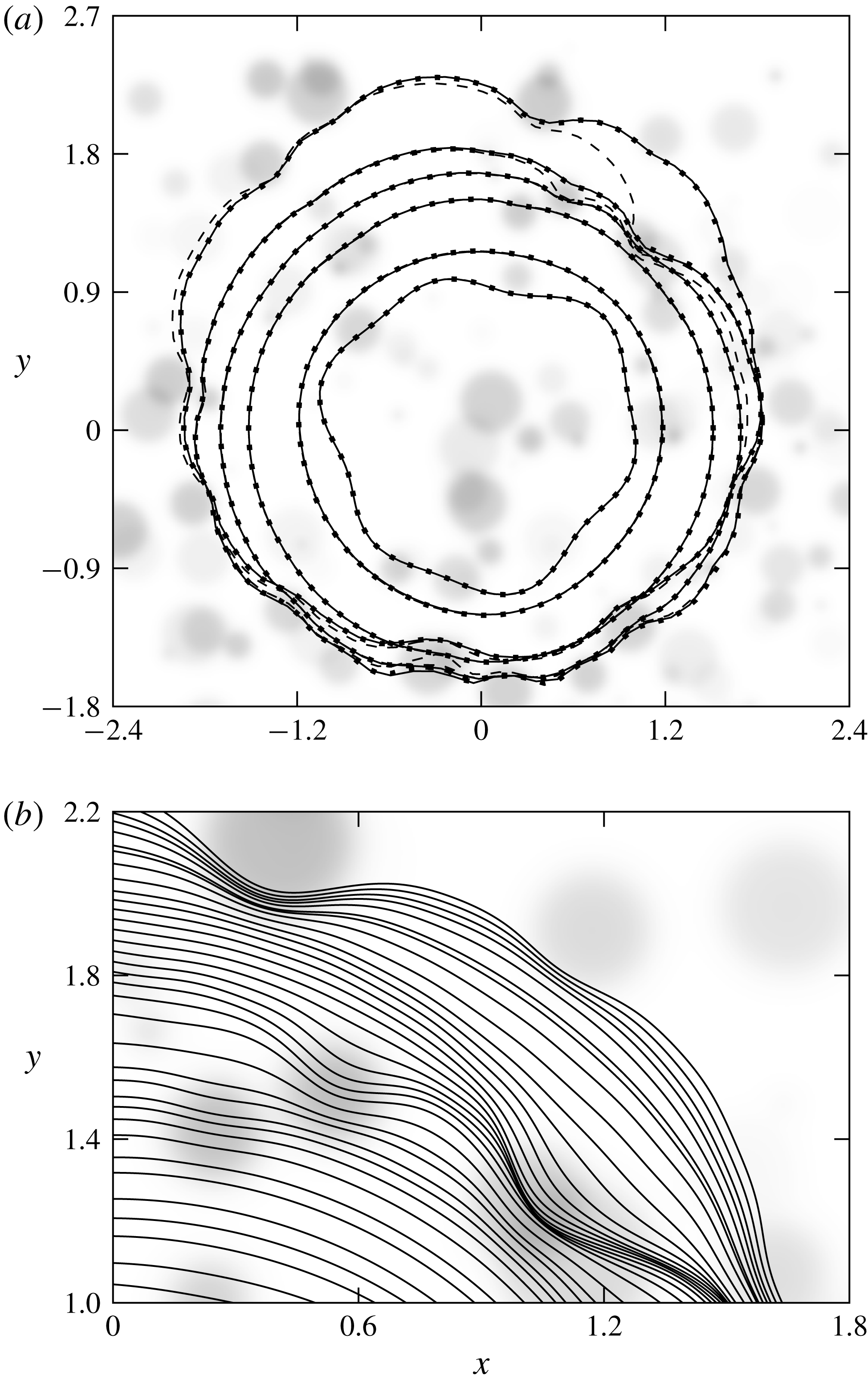
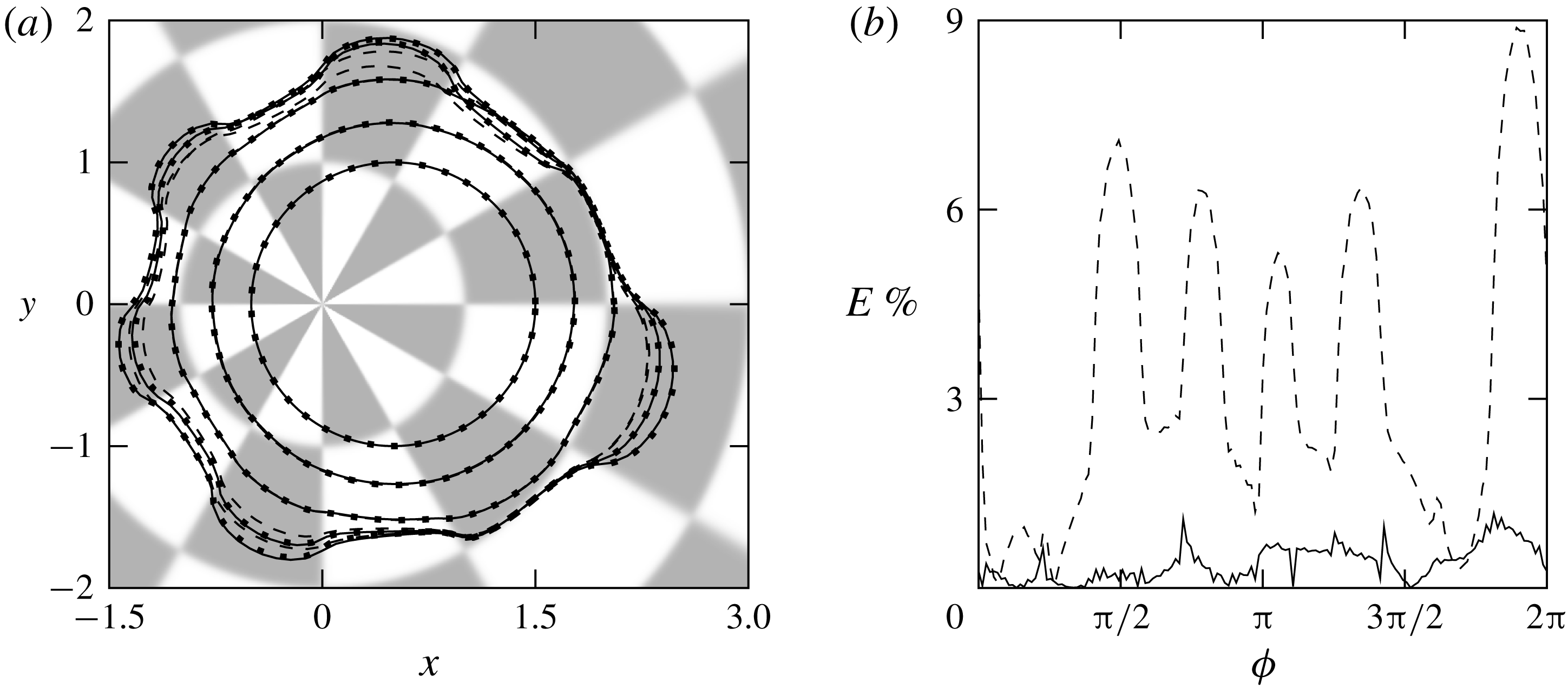
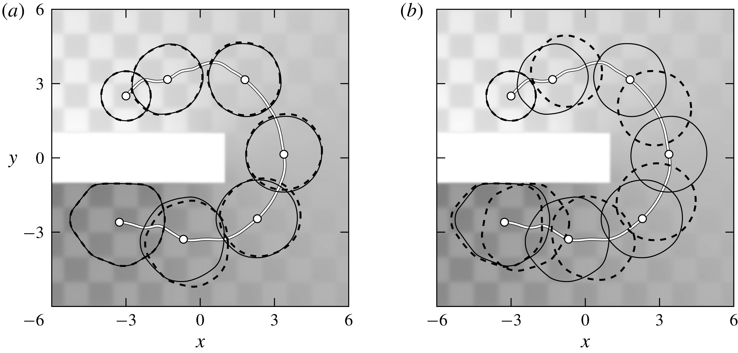
1 Introduction
The evolution of a contact line, formed by the intersection of a fluid–fluid interface with a solid substrate, is crucial in a broad spectrum of natural and industrial processes (for reviews, see Teh et al. Reference Teh, Lin, Hung and Lee2008, Bonn et al. Reference Bonn, Eggers, Indekeu, Meunier and Rolley2009, and references therein). Yet, moving contact line modelling is highly non-trivial due to the inherent multiscale nature of the associated phenomena, which span multiple scales, from the nanoscale near the contact line and the micro-/mesoscale features of the substrate to the macroscale characterising the bulk of the liquid (see e.g. Snoeijer & Andreotti Reference Snoeijer and Andreotti2013).
A large body of work has been devoted to unravelling the dynamics of contact lines when the wetting properties of the substrate exhibit spatial variations. The ultimate aim is to inform strategies for controlling droplet behaviour in applications. This work has been primarily experimental, demonstrating pinning and stick–slip behaviours, as well as the possibility of unidirectional motion. For instance, pinning was reported by Cubaud & Fermigier (Reference Cubaud and Fermigier2004) for substrates containing localised defects of lower wettability prepared by microphotolithography. The most commonly studied configuration is arguably the case of substrates decorated by stripes of alternating wettability (see e.g. Bliznyuk et al. Reference Bliznyuk, Vereshchagina, Kooij and Poelsema2009, Jansen et al. Reference Jansen, Sotthewes, Ganser, Teichert, Zandvliet and Kooij2012, Jansen et al. Reference Jansen, Sotthewes, Ganser, Zandvliet, Teichert and Kooij2014, Damle & Rykaczewski Reference Damle and Rykaczewski2017, as well as Ghosh et al. Reference Ghosh, Beaini, Zhang, Ganguly and Megaridis2014 for an application in dropwise condensation). When wettability contrasts are sufficiently strong for such substrates, the droplet stretches and spreads parallel to the stripes and becomes elongated in the long-time limit. Also related to these configurations is the work of Darhuber, Troian & Reisner (Reference Darhuber, Troian and Reisner2001) who conducted experiments with long and thin strips of liquid on a hydrophilic stripe (see also Brinkmann & Lipowsky Reference Brinkmann and Lipowsky2002, for a related theoretical study on the associated equilibrium solutions). Unidirectional droplet transport can be observed when the substrate is decorated with a wettability gradient and, if the gradient is sufficiently strong, the droplet may overcome the force of gravity and move uphill on an inclined plane (see e.g. the experiments by Chaudhury & Whitesides Reference Chaudhury and Whitesides1992, Ichimura, Sang-Keun & Nakagawa Reference Ichimura, Sang-Keun and Nakagawa2000, Moumen, Subramanian & McLaughlin Reference Moumen, Subramanian and McLaughlin2006, Ito et al. Reference Ito, Heydari, Hashimoto, Konno, Hirasawa, Hori, Kurita and Nakajima2007, as well as the theoretical results by Brochard Reference Brochard1989, Subramanian, Moumen & McLaughlin Reference Subramanian, Moumen and McLaughlin2005, Pismen Reference Pismen2006).
In this study we undertake a combined numerical and analytical investigation of droplet motion on chemically heterogeneous substrates. Analytical progress in this problem is possible under the assumption that the dynamics is slow, so that the problem may be treated in a quasi-static manner (Lacey Reference Lacey1982, Hocking Reference Hocking1983). Moreover, the assumptions of a small interface slope, strong surface tension effects and negligible inertia reduce the governing equations, and wall and free surface boundary conditions to a single evolution equation for the droplet thickness. The aforementioned separation of scales then allows for analytical scrutiny of the equation based on the method of matched asymptotic expansions. These ideas have been previously explored in two-dimensional and axisymmetric geometries with various complexities to obtain simplified, lower-dimensional models that were shown to typically exhibit excellent agreement with numerical solutions to the full problems; see e.g. Savva & Kalliadasis (Reference Savva and Kalliadasis2009, Reference Savva and Kalliadasis2011, Reference Savva and Kalliadasis2012, Reference Savva and Kalliadasis2013, Reference Savva and Kalliadasis2014), Vellingiri, Savva & Kalliadasis (Reference Vellingiri, Savva and Kalliadasis2011), Oliver et al. (Reference Oliver, Whiteley, Saxton, Vella, Zubkov and King2015), Saxton et al. (Reference Saxton, Whiteley, Vella and Oliver2016) and Savva, Rednikov & Colinet (Reference Savva, Rednikov and Colinet2017). In contrast, the fully three-dimensional setting has received less attention, especially when the contact line becomes perturbed due to heterogeneities. Greenspan (Reference Greenspan1978) and Greenspan & McCay (Reference Greenspan and McCay1981) offered the first analyses of this configuration by considering weakly perturbed contact lines and assuming a priori that the velocity of the contact line,
 $\boldsymbol{v}$
, satisfies
 $$\begin{eqnarray}\boldsymbol{v}=-k(\unicode[STIX]{x2202}_{\unicode[STIX]{x1D708}}h|_{C}+\unicode[STIX]{x1D717}_{\ast })\unicode[STIX]{x1D742},\end{eqnarray}$$
where
 $\unicode[STIX]{x2202}_{\unicode[STIX]{x1D708}}h|_{C}$
denotes the normal derivative of the free surface evaluated along the contact line
 $C$
,
 $\unicode[STIX]{x1D717}_{\ast }$
corresponds to the local contact angle along the contact line prescribed by the heterogeneities,
 $\unicode[STIX]{x1D742}$
is the outward unit normal to the contact line and
 $k>0$
is some constant of proportionality. The term
 $\unicode[STIX]{x2202}_{\unicode[STIX]{x1D708}}h|_{C}=-|\unicode[STIX]{x1D735}h|_{C}=\unicode[STIX]{x1D703}$
in (1.1) corresponds to the apparent contact angle, which may be viewed as an extrapolated angle near the contact line based on the shape of the bulk of the droplet. This angle can be evaluated by solving the corresponding Young–Laplace equation, which reduces to the Poisson equation in the long-wave limit (Lacey Reference Lacey1982, Glasner Reference Glasner2005). Note that this approach has been invoked in related problems (e.g. for vibrated drops on inclined planes see Benilov Reference Benilov2011, Benilov & Cummins Reference Benilov and Cummins2013), but it is important to emphasise that it is not based on matched asymptotics, since a product of the asymptotic procedure is precisely an expression for the contact line velocity. Lacey (Reference Lacey1982) was the first to develop a general asymptotic procedure for fully three-dimensional drops and obtained the normal velocity of the contact line in the form
 $$\begin{eqnarray}\boldsymbol{v}\boldsymbol{\cdot }\unicode[STIX]{x1D742}=\frac{\unicode[STIX]{x1D717}_{\ast }^{3}-\unicode[STIX]{x1D703}^{3}}{3\ln \unicode[STIX]{x1D706}},\end{eqnarray}$$
where
 $\unicode[STIX]{x1D706}$
is the slip length (the normal velocity is the crucial quantity of interest as it is widely accepted that fronts and interfaces move in a direction normal to themselves, e.g. Meron Reference Meron1992). Equation (1.2) is cast in non-dimensional form according to the scalings introduced in § 2 and corresponds to the first term in the asymptotic expansion for the normal velocity as
 $\unicode[STIX]{x1D706}\rightarrow 0$
. Including the next-order correction is highly non-trivial, but it is necessary for satisfactory results given that the leading-order result, (1.2), would asymptotically remain the same if
 $\unicode[STIX]{x1D706}$
were to be replaced by a multiple of itself (Hocking Reference Hocking1983). A two-term expansion has been produced in the two-dimensional version of the problem by Vellingiri et al. (Reference Vellingiri, Savva and Kalliadasis2011), but such analysis is presently lacking for the problem in three dimensions. Thus, the key contribution of the present study is building upon previous analyses in two dimensions to extend Lacey’s work in order to incorporate these higher-order corrections in the matching procedure and resolve the aforementioned shortcoming of matching with just the leading-order logarithmic term in the expansion.
We also compare the predictions of the asymptotic analysis with the solutions to the full problem obtained from a highly accurate numerical scheme based on pseudospectral collocation for the spatial discretisation and the method of lines for time stepping. To date, a number of different methodologies have been utilised to simulate contact lines in the presence of heterogeneities and other complexities (see the review of Sui, Ding & Spelt (Reference Sui, Ding and Spelt2014) and the references therein). These include, for example, the works of Schwartz (Reference Schwartz1998) and Schwartz & Eley (Reference Schwartz and Eley1998), who used finite differences to simulate a long-wave model with a disjoining pressure term, as well as simulations based on the lattice Boltzmann method for mesoscopic droplets (see e.g. Dupuis & Yeomans Reference Dupuis and Yeomans2004, Kusumaatmaja & Yeomans Reference Kusumaatmaja and Yeomans2007, Jansen et al. Reference Jansen, Sotthewes, Ganser, Zandvliet, Teichert and Kooij2014). Noteworthy also is the work of Glasner (Reference Glasner2005) who assumed that the dynamics of thin drops exhibit quasi-static behaviour and solved for the shape of the contact line using the boundary integral method in conjunction with an imposed form for the normal velocity of the contact line, which effectively corresponds to (1.2) with time rescaled. This connection of Glasner’s method and Lacey’s asymptotics is highlighted further in this work, demonstrating how such an approach can lead to more favourable comparisons with the full problem.
In the next section, a brief overview of the long-wave model adopted is presented, together with its corresponding conditions. A coordinate transformation is presented in § 3, which is utilised in treating the problem both numerically and analytically. The details of the matched asymptotic analysis are given in § 4, where we derive a set of equations for the evolution of the contact line. In § 5 we discuss briefly the numerical schemes we adopt in solving the governing partial differential equation (PDE), the equations obtained from matching as well as a hybrid method, which combines the boundary integral method with the results of the asymptotic analysis in order to capture accurately strongly deformed contact lines. To assess the regime of validity of our analysis, a number of illustrative cases comparing the solutions to the full problem and the equations of the asymptotic analysis are presented in § 6. A summary and some final remarks for future work are offered in § 7.
2 Long-wave model
Consider the motion of a partially wetting droplet on a substrate on the
 $X$
–
 $Y$
plane. The substrate is heterogeneous with regions of varying wettability, as prescribed by a spatially varying equilibrium contact angle through an imposed function
 $\unicode[STIX]{x1D6E9}(X,Y)$
, assumed to be small. The assumptions of the long-wave theory, which involves a small-slope expansion of the Stokes equations, lead to a single nonlinear PDE for the evolution of the thickness of the droplet,
 $H(X,Y,T)$
at position
 $(X,Y)$
and time
 $T$
(Greenspan Reference Greenspan1978).
Central to the description of contact line dynamics is the use of some model to treat the non-integrable stress singularity that would occur at a moving contact line if a no-slip condition is applied on the substrate (Huh & Scriven Reference Huh and Scriven1971). To alleviate this singularity, we utilise one of the slip models examined by Haley & Miksis (Reference Haley and Miksis1991) and Diez, Kondic & Bertozzi (Reference Diez, Kondic and Bertozzi2000) for two-dimensional droplets on homogeneous substrates (see also Ruckenstein & Dunn Reference Ruckenstein and Dunn1977), which prescribes the velocity of the fluid along the substrate,
 $\boldsymbol{U}$
, according to
 $$\begin{eqnarray}\boldsymbol{U}=\frac{\unicode[STIX]{x1D6EC}^{2}}{\unicode[STIX]{x1D707}H}\boldsymbol{n}\boldsymbol{\cdot }\unicode[STIX]{x1D64E}\boldsymbol{\cdot }\boldsymbol{t},\end{eqnarray}$$
where
 $\unicode[STIX]{x1D6EC}$
is the slip length,
 $\unicode[STIX]{x1D707}$
is the viscosity of the fluid,
 $\unicode[STIX]{x1D64E}$
is the viscous stress tensor, with
 $\boldsymbol{n}$
and
 $\boldsymbol{t}$
being the unit normal and tangent vectors to the substrate, respectively. A slip model regularises the divergent viscous shear stress in the vicinity of the contact line, while its contributions elsewhere in the bulk of the liquid are negligibly small. For simplicity, we assume that
 $\unicode[STIX]{x1D6EC}$
is constant everywhere, although the analysis we will present is expected to hold for a spatially varying
 $\unicode[STIX]{x1D6EC}$
, as long as it varies at length scales that are much longer compared to its size. Let us also emphasise that here we have decided against using the arguably more popular Navier slip model,
 $$\begin{eqnarray}\boldsymbol{U}=\frac{\unicode[STIX]{x1D6EC}}{\unicode[STIX]{x1D707}}\boldsymbol{n}\boldsymbol{\cdot }\unicode[STIX]{x1D64E}\boldsymbol{\cdot }\boldsymbol{t},\end{eqnarray}$$
solely because its proper numerical implementation is considerably more difficult and requires a specialised scheme. This is a consequence of the fact that the pressure has a logarithmic singularity along the contact line for the Navier slip model, which is nevertheless integrable and leads to a finite force (for the two-dimensional version of the present problem, see the scheme used by Vellingiri et al.
Reference Vellingiri, Savva and Kalliadasis2011). In contrast, the advantage of the model in (2.1) is that it alleviates the pressure singularity, thus regularising the total shear stress (Sibley et al.
Reference Sibley, Nold, Savva and Kalliadasis2015b
). It is also important to mention that had we used the Navier slip model, the asymptotic analysis would have been identical to the one presented here at the orders at which matching is performed and for the boundary conditions utilised. This conclusion, which has been shown to hold for the two-dimensional case (see e.g. Savva & Kalliadasis Reference Savva and Kalliadasis2011), is expected to pertain to three dimensions as well, subject to the caveat that the contact line must be assumed to vary at length scales that are much longer than
 $\unicode[STIX]{x1D6EC}$
(see also § 4.1). In fact, generalisations are also possible for a wide variety of other contact line models. As seen in previous works (see e.g. King Reference King, King and Shikhmurzaev2001, Eggers Reference Eggers2005, Sibley, Savva & Kalliadasis Reference Sibley, Savva and Kalliadasis2012, Sibley et al.
Reference Sibley, Nold, Savva and Kalliadasis2013, Sibley et al.
Reference Sibley, Nold, Savva and Kalliadasis2015b
), such asymptotic analyses can be straightforwardly adapted to hold for other contact line models by suitably choosing the microscopic scale (in this case
 $\unicode[STIX]{x1D6EC}$
) and formally linking it with the asymptotics in the vicinity of the contact line.
The governing PDE is obtained by standard arguments presented in earlier works and discussed before, i.e. strong surface tension, negligible inertial effects and small contact angles (see e.g. Greenspan Reference Greenspan1978, Hocking Reference Hocking1983). In the end, we find that
 $H(X,Y,T)$
must satisfy
 $$\begin{eqnarray}3\unicode[STIX]{x1D707}\unicode[STIX]{x2202}_{T}H+\unicode[STIX]{x1D70E}\unicode[STIX]{x1D735}\boldsymbol{\cdot }\{H(H^{2}+3\unicode[STIX]{x1D6EC}^{2})\unicode[STIX]{x1D735}\unicode[STIX]{x1D6FB}^{2}H\}=0,\end{eqnarray}$$
where
 $\unicode[STIX]{x1D70E}$
is the surface tension. Gravitational effects are also neglected here. This is done by assuming that the droplet’s characteristic length is much smaller than the capillary length
 $\sqrt{\unicode[STIX]{x1D70E}/(\unicode[STIX]{x1D70C}g)}$
, where
 $g$
is the acceleration due to gravity. We then have a free-boundary problem, where, apart from the droplet thickness, it is also necessary to utilise another PDE for the evolution of the contact line,
 $C$
. Naturally, since the free surface of the droplet meets the substrate along
 $C$
, we must have
 $$\begin{eqnarray}H|_{C}=0.\end{eqnarray}$$
Additionally, we also have a contact angle condition, which prescribes the local contact angle according to
 $\unicode[STIX]{x1D6E9}(X,Y)$
, namely we require
 $$\begin{eqnarray}|\unicode[STIX]{x1D735}H|_{C}=\tan \unicode[STIX]{x1D6E9}|_{C}.\end{eqnarray}$$
The final condition must be of kinematic type to describe the contact line deformations. This can be deduced from (2.1) evaluated along the contact line, which, in long-wave form, becomes
 $$\begin{eqnarray}\boldsymbol{U}|_{C}=\frac{\unicode[STIX]{x1D70E}}{\unicode[STIX]{x1D707}}\unicode[STIX]{x1D6EC}^{2}\unicode[STIX]{x1D735}\unicode[STIX]{x1D6FB}^{2}H|_{C}.\end{eqnarray}$$
The evolution of the contact line according to (2.6) is consistent with the asymptotics of
 $H$
as the contact line is approached and ensures that the volume of the droplet is conserved at all times. Thus, by letting
 $\boldsymbol{C}(s,T)$
denote the position vector of the closed curve that describes the contact line at time
 $T$
as parametrised by
 $s$
, we require that the velocity of fluid particles at the contact line matches the velocity of the contact line, namely
 $$\begin{eqnarray}\boldsymbol{U}|_{C}=\frac{\text{d}\boldsymbol{C}}{\text{d}T}.\end{eqnarray}$$
Hence, to the level of approximation offered by our model, this view of
 $C$
as a material curve is a reasonable one and is compatible with the zero-mass-flux condition along
 $C$
(Young Reference Young, Brown and Davis1994). Since we know that
 $$\begin{eqnarray}\frac{\text{d}\boldsymbol{C}}{\text{d}T}\boldsymbol{\cdot }\unicode[STIX]{x1D742}=\unicode[STIX]{x2202}_{T}\boldsymbol{C}\boldsymbol{\cdot }\unicode[STIX]{x1D742},\end{eqnarray}$$
we combine (2.6)–(2.8) to obtain a PDE for
 $\boldsymbol{C}(s,T)$
that closes the problem
 $$\begin{eqnarray}\unicode[STIX]{x2202}_{T}\boldsymbol{C}\boldsymbol{\cdot }\unicode[STIX]{x1D742}=\frac{\unicode[STIX]{x1D70E}}{\unicode[STIX]{x1D707}}\unicode[STIX]{x1D6EC}^{2}\unicode[STIX]{x1D735}\unicode[STIX]{x1D6FB}^{2}H|_{C}\boldsymbol{\cdot }\unicode[STIX]{x1D742}.\end{eqnarray}$$
Hence, the droplet dynamics is fully determined from the evolution of
 $H(X,Y,T)$
and
 $\boldsymbol{C}(s,T)$
, by solving (2.3) and (2.9) subject to an initial droplet shape and the boundary conditions (2.4) and (2.5). To proceed, we introduce the non-dimensional independent variables
 $$\begin{eqnarray}x=\frac{X}{L}\quad y=\frac{Y}{L}\quad \text{and}\quad t=\frac{\unicode[STIX]{x1D70E}\tan ^{3}\unicode[STIX]{x1D6E9}_{0}T}{3\unicode[STIX]{x1D707}L},\end{eqnarray}$$
where
 $\unicode[STIX]{x1D6E9}_{0}$
is some reference angle (e.g. the mean contact angle of the substrate) and
 $L$
is a characteristic scale for the size of the droplet, which satisfies
 $2\unicode[STIX]{x03C0}L^{3}\tan \unicode[STIX]{x1D6E9}_{0}=V$
, where
 $V$
is the droplet volume. Based on these scales, we use the variables
 $$\begin{eqnarray}h=\frac{H}{L\tan \unicode[STIX]{x1D6E9}_{0}},\quad \boldsymbol{c}=\frac{\boldsymbol{C}}{L},\quad \unicode[STIX]{x1D717}=\frac{\tan \unicode[STIX]{x1D6E9}}{\tan \unicode[STIX]{x1D6E9}_{0}},\quad \unicode[STIX]{x1D706}=\frac{\sqrt{3}\unicode[STIX]{x1D6EC}}{L\tan \unicode[STIX]{x1D6E9}_{0}}\end{eqnarray}$$
to write down the governing PDEs, (2.3) and (2.9), and conditions, (2.4) and (2.5), as
 $$\begin{eqnarray}\displaystyle & \displaystyle \unicode[STIX]{x2202}_{t}h+\unicode[STIX]{x1D735}\boldsymbol{\cdot }[h(h^{2}+\unicode[STIX]{x1D706}^{2})\unicode[STIX]{x1D735}\unicode[STIX]{x1D6FB}^{2}h]=0, & \displaystyle\end{eqnarray}$$
 $$\begin{eqnarray}\displaystyle & \displaystyle (\unicode[STIX]{x2202}_{t}\boldsymbol{c}-\unicode[STIX]{x1D706}^{2}\unicode[STIX]{x1D735}\unicode[STIX]{x1D6FB}^{2}h|_{C})\boldsymbol{\cdot }\unicode[STIX]{x1D742}=0, & \displaystyle\end{eqnarray}$$
 $$\begin{eqnarray}\displaystyle & \displaystyle h|_{C}=0, & \displaystyle\end{eqnarray}$$
 $$\begin{eqnarray}\displaystyle & \displaystyle |\unicode[STIX]{x1D735}h|_{C}=\unicode[STIX]{x1D717}|_{C}, & \displaystyle\end{eqnarray}$$
 $x$
–
 $y$
coordinate system. The numerical solution to the problem described by (2.12) is non-trivial, as it requires a carefully developed numerical scheme that is able to capture the boundary layers around the freely moving contact line.
3 Coordinate transformation
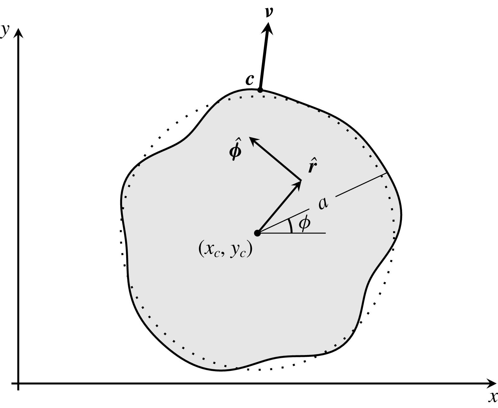
Top view of the problem geometry in non-dimensional units. The contact line (thick curve) is a perturbation from a circular contact line (dotted curve). The shaded area corresponds to the droplet footprint, whose boundary is described by the distance
 $a(\unicode[STIX]{x1D719},t)$
from its centroid,
 $(x_{c}(t),y_{c}(t))$
. The vectors
 $\hat{\boldsymbol{r}}$
and
 $\hat{\unicode[STIX]{x1D753}}$
denote the unit normal vectors in the radial and azimuthal directions in the moving frame, respectively;
 $\unicode[STIX]{x1D742}$
is the outward unit normal to the contact line at
 $\boldsymbol{c}$
.

To proceed with the analysis and numerics, (2.12) is cast in a suitable coordinate system. Due to the nature of the problem geometry, the use of polar coordinates is arguably the natural choice for this system, and should be utilised in a moving frame in order to be able to trace droplets undergoing long excursions from their initial positions (see figure 1). More specifically, we introduce a coordinate transformation that maps every point in the domain of the problem, defined by the
 $x$
and
 $y$
coordinates of the contact area, to the unit disk described by the
 $(r,\unicode[STIX]{x1D719})$
polar coordinates using
 $$\begin{eqnarray}\displaystyle & \displaystyle x=x_{c}(t)+a(\unicode[STIX]{x1D719},t)r\cos \unicode[STIX]{x1D719}, & \displaystyle\end{eqnarray}$$
 $$\begin{eqnarray}\displaystyle & \displaystyle y=y_{c}(t)+a(\unicode[STIX]{x1D719},t)r\sin \unicode[STIX]{x1D719}, & \displaystyle\end{eqnarray}$$
 $0\leqslant r\leqslant 1$
,
 $0\leqslant \unicode[STIX]{x1D719}<2\unicode[STIX]{x03C0}$
. Here,
 $(x_{c}(t),y_{c}(t))$
corresponds to the origin of the moving frame at time
 $t$
and
 $a(\unicode[STIX]{x1D719},t)$
is the distance of a point on the contact line from
 $(x_{c}(t),y_{c}(t))$
(see figure 1). With this change of variables, the irregularly shaped contact line is mapped to the unit circle, thus transforming the free-boundary problem to a problem with fixed boundaries. As it turns out, dealing with a fixed boundary problem is not only desirable for the numerics but also for the analysis that follows. Hence, as
 $r\rightarrow 1$
, we approach the contact line
 $\boldsymbol{x}=\boldsymbol{c}$
, where
 $$\begin{eqnarray}\boldsymbol{c}(\unicode[STIX]{x1D719},t)=(x_{c}(t)+a(\unicode[STIX]{x1D719},t)\cos \unicode[STIX]{x1D719},y_{c}(t)+a(\unicode[STIX]{x1D719},t)\sin \unicode[STIX]{x1D719}).\end{eqnarray}$$
An important assumption of this parametrisation is that the contact line deforms sufficiently weakly to allow for
 $a(\unicode[STIX]{x1D719},t)$
to be a one-to-one function of the polar angle in the interval
 $0\leqslant \unicode[STIX]{x1D719}<2\unicode[STIX]{x03C0}$
.
It is a matter of straightforward algebra to show that (2.12a ) transforms to
 $$\begin{eqnarray}\displaystyle & & \displaystyle \unicode[STIX]{x2202}_{t}h-\frac{1}{a}\left[{\dot{x}}_{c}\cos \unicode[STIX]{x1D719}+{\dot{y}}_{c}\sin \unicode[STIX]{x1D719}+r\unicode[STIX]{x2202}_{t}a+\frac{\unicode[STIX]{x2202}_{\unicode[STIX]{x1D719}}a}{a}({\dot{x}}_{c}\sin \unicode[STIX]{x1D719}-{\dot{y}}_{c}\cos \unicode[STIX]{x1D719})\right]\unicode[STIX]{x2202}_{r}h\nonumber\\ \displaystyle & & \displaystyle \quad +\,\frac{{\dot{x}}_{c}\sin \unicode[STIX]{x1D719}-{\dot{y}}_{c}\cos \unicode[STIX]{x1D719}}{ar}\unicode[STIX]{x2202}_{\unicode[STIX]{x1D719}}h+\unicode[STIX]{x1D735}\boldsymbol{\cdot }[h(h^{2}+\unicode[STIX]{x1D706}^{2})\unicode[STIX]{x1D735}\unicode[STIX]{x1D6FB}^{2}h]=0,\end{eqnarray}$$
where the dot denotes differentiation with respect to
 $t$
. The gradient operator becomes
 $$\begin{eqnarray}\unicode[STIX]{x1D735}(\cdot )=\hat{\boldsymbol{r}}\frac{1}{a}\unicode[STIX]{x2202}_{r}(\cdot )+\hat{\unicode[STIX]{x1D753}}\left[\frac{1}{ar}\unicode[STIX]{x2202}_{\unicode[STIX]{x1D719}}(\cdot )-\frac{\unicode[STIX]{x2202}_{\unicode[STIX]{x1D719}}a}{a^{2}}\unicode[STIX]{x2202}_{r}(\cdot )\right],\end{eqnarray}$$
where
 $\hat{\boldsymbol{r}}$
and
 $\hat{\unicode[STIX]{x1D753}}$
denote the unit normal vectors in the radial and azimuthal directions in the moving frame, respectively, and
 $(\cdot )$
denotes the placeholder for the operand. Similarly, the Laplacian is written in the form
 $$\begin{eqnarray}\displaystyle \unicode[STIX]{x1D6FB}^{2}(\cdot ) & = & \displaystyle \frac{1}{a^{2}}\left[1+\left(\frac{\unicode[STIX]{x2202}_{\unicode[STIX]{x1D719}}a}{a}\right)^{2}\right]\unicode[STIX]{x2202}_{r}^{2}(\cdot )+\frac{1}{a^{2}r^{2}}\unicode[STIX]{x2202}_{\unicode[STIX]{x1D719}}^{2}(\cdot )-2\frac{\unicode[STIX]{x2202}_{\unicode[STIX]{x1D719}}a}{a^{3}r}\unicode[STIX]{x2202}_{\unicode[STIX]{x1D719}}\unicode[STIX]{x2202}_{r}(\cdot )\nonumber\\ \displaystyle & & \displaystyle +\,\frac{1}{a^{2}r}\left[1-\frac{\unicode[STIX]{x2202}_{\unicode[STIX]{x1D719}}^{2}a}{a}+2\left(\frac{\unicode[STIX]{x2202}_{\unicode[STIX]{x1D719}}a}{a}\right)^{2}\right]\unicode[STIX]{x2202}_{r}(\cdot ).\end{eqnarray}$$
Obtaining the last term of (3.3) in terms of the
 $r$
- and
 $\unicode[STIX]{x1D719}$
-derivatives is a standard exercise in calculus, although the final expression is rather long and cumbersome to include here. Condition (2.12b
) yields a PDE that governs the evolution of
 $a(\unicode[STIX]{x1D719},t)$
. Using the outward unit normal to the contact line
 $$\begin{eqnarray}\unicode[STIX]{x1D742}=\frac{a\hat{\boldsymbol{r}}-\unicode[STIX]{x2202}_{\unicode[STIX]{x1D719}}a\hat{\unicode[STIX]{x1D753}}}{\sqrt{a^{2}+(\unicode[STIX]{x2202}_{\unicode[STIX]{x1D719}}a)^{2}}},\end{eqnarray}$$
we cast (2.12b ) in the form
 $$\begin{eqnarray}({\dot{x}}_{c}\cos \unicode[STIX]{x1D719}+{\dot{y}}_{c}\sin \unicode[STIX]{x1D719}+\unicode[STIX]{x2202}_{t}a)a-({\dot{y}}_{c}\cos \unicode[STIX]{x1D719}-{\dot{x}}_{c}\sin \unicode[STIX]{x1D719})\unicode[STIX]{x2202}_{\unicode[STIX]{x1D719}}a=W,\end{eqnarray}$$
where
 $$\begin{eqnarray}W(\unicode[STIX]{x1D719},t)=\unicode[STIX]{x1D706}^{2}\left.\left\{\left[1+\left(\frac{\unicode[STIX]{x2202}_{\unicode[STIX]{x1D719}}a}{a}\right)^{2}\right]\unicode[STIX]{x2202}_{r}\unicode[STIX]{x1D6FB}^{2}h-\frac{\unicode[STIX]{x2202}_{\unicode[STIX]{x1D719}}a}{a}\unicode[STIX]{x2202}_{\unicode[STIX]{x1D719}}\unicode[STIX]{x1D6FB}^{2}h\right\}\right|_{r=1}.\end{eqnarray}$$
Under the coordinate transformation, (3.1), condition (2.12c ) requires
 $$\begin{eqnarray}h(1,\unicode[STIX]{x1D719},t)=0.\end{eqnarray}$$
Lastly, condition (2.12d ) becomes
 $$\begin{eqnarray}\unicode[STIX]{x2202}_{r}h|_{r=1}=-\frac{a\unicode[STIX]{x1D717}_{\ast }}{\sqrt{1+\left(\displaystyle \frac{\unicode[STIX]{x2202}_{\unicode[STIX]{x1D719}}a}{a}\right)^{2}}},\end{eqnarray}$$
where
 $\unicode[STIX]{x1D717}_{\ast }=\unicode[STIX]{x1D717}|_{C}=\unicode[STIX]{x1D717}(x_{c}+a\cos \unicode[STIX]{x1D719},y_{c}+a\sin \unicode[STIX]{x1D719})$
. Clearly, there is some arbitrariness in the choice of
 $x_{c}$
and
 $y_{c}$
. Here we assume that the origin of the moving frame is always at the centroid of the contact area, which requires that we must have at all times
 $$\begin{eqnarray}\int _{0}^{2\unicode[STIX]{x03C0}}a^{3}\cos \unicode[STIX]{x1D719}\,\text{d}\unicode[STIX]{x1D719}=\int _{0}^{2\unicode[STIX]{x03C0}}a^{3}\sin \unicode[STIX]{x1D719}\,\text{d}\unicode[STIX]{x1D719}=0.\end{eqnarray}$$
These integral conditions, however, define
 $x_{c}$
and
 $y_{c}$
implicitly. To obtain an explicit expression for
 ${\dot{x}}_{c}$
, multiply (3.7) by
 $a\cos \unicode[STIX]{x1D719}$
and integrate from 0 to
 $2\unicode[STIX]{x03C0}$
, so that we obtain
 $$\begin{eqnarray}{\dot{x}}_{c}=\frac{2\displaystyle \int _{0}^{2\unicode[STIX]{x03C0}}aW\cos \unicode[STIX]{x1D719}\,\text{d}\unicode[STIX]{x1D719}}{\displaystyle \int _{0}^{2\unicode[STIX]{x03C0}}a^{2}\,\text{d}\unicode[STIX]{x1D719}},\end{eqnarray}$$
by making use of (3.11). Similarly, an expression for
 ${\dot{y}}_{c}$
can be found by multiplying (3.7) by
 $a\sin \unicode[STIX]{x1D719}$
and integrating from 0 to
 $2\unicode[STIX]{x03C0}$
and we find
 $$\begin{eqnarray}{\dot{y}}_{c}=\frac{2\displaystyle \int _{0}^{2\unicode[STIX]{x03C0}}aW\sin \unicode[STIX]{x1D719}\,\text{d}\unicode[STIX]{x1D719}}{\displaystyle \int _{0}^{2\unicode[STIX]{x03C0}}a^{2}\,\text{d}\unicode[STIX]{x1D719}}.\end{eqnarray}$$
With these last two conditions, we close the problem of obtaining the solution to (2.12) under the new coordinate system. In other words, we need to solve (3.3), (3.7), (3.12) and (3.13) subject to an initial condition and the boundary conditions (3.9) and (3.10), noting that the precludes initial condition must satisfy
 $$\begin{eqnarray}\int _{0}^{2\unicode[STIX]{x03C0}}a^{2}(\unicode[STIX]{x1D719},0)\int _{0}^{1}rh(r,\unicode[STIX]{x1D719},0)\,\text{d}r\,\text{d}\unicode[STIX]{x1D719}=2\unicode[STIX]{x03C0},\end{eqnarray}$$
with our chosen non-dimensionalisation. Clearly the complexity of the problem precludes a fully analytical treatment. At the same time, capturing the boundary layers that are present near the contact line make the problem rather stiff, especially for very small values of
 $\unicode[STIX]{x1D706}$
. Hence, analytical progress is desirable, both in order to mitigate the high computational cost of the full problem and, importantly, to extract some physical insights from a highly complex problem.
4 Analysis
Here we perform an asymptotic analysis in the small-slip limit and under the assumption that
 $\unicode[STIX]{x2202}_{\unicode[STIX]{x1D719}}a\ll a$
, which also ensures that the contact line varies at length scales that are longer than
 $\unicode[STIX]{x1D706}$
. Just as in two-dimensional studies (Lacey Reference Lacey1982, Hocking Reference Hocking1983), our analysis is formally valid on the slow time scale
 $t=O(|\text{ln}\,\unicode[STIX]{x1D706}|)$
as
 $\unicode[STIX]{x1D706}\rightarrow 0$
. We consider a truncated Fourier series expansion of
 $a(\unicode[STIX]{x1D719},t)$
, whereby we discard short-wavelength harmonics, writing
 $$\begin{eqnarray}a(\unicode[STIX]{x1D719},t)=\mathop{\sum }_{m=0}^{M}a_{m}(t)\text{e}^{\text{i}m\unicode[STIX]{x1D719}},\end{eqnarray}$$
where
 $a_{m}$
with
 $m=0,1,\ldots ,M$
are generally complex functions of
 $t$
to be determined and
 $M$
is a large positive integer to be defined more precisely later. It is important to note that in (4.1) and in the discussion that follows, all expressions containing complex exponentials are considered with the understanding that the imaginary part is discarded, analogously to the ‘normal modes’ of linear stability theory. The contact line is assumed to be nearly circular with
 $|a_{m}(t)|\ll a_{0}(t)$
and we keep only the linear terms in the non-axisymmetric components of
 $a(\unicode[STIX]{x1D719},t)$
. Although this approach is reminiscent of linear stability theory, its distinguishing characteristic is that we consider perturbations from dynamic states, thus leaving all time dependences arbitrary. In contrast, normal modes in linear stability theory are perturbations from steady states with an exponential dependence on time. Recalling that in § 3 we chose the centroid of the contact area to be located at the origin of the moving frame, using (4.1) in (3.11) and keeping only the leading-order terms, we readily deduce that
 $\text{Re}(a_{1})+O(a_{m}^{2})=0$
and
 $\text{Im}(a_{1})+O(a_{m}^{2})=0$
. This implies that if
 $(x_{c}(t),y_{c}(t))$
evolves such that the first harmonic of
 $a(\unicode[STIX]{x1D719},t)$
is always zero, then this is, at leading order, equivalent to having
 $(x_{c}(t),y_{c}(t))$
at the centroid of the contact area. Here, we require that
 $a_{1}(t)\equiv 0$
, which is an alternative, equally valid way to choose the origin of the moving frame.
The aim of the analysis that follows is to obtain a set of evolution equations for
 $x_{c}$
,
 $y_{c}$
and
 $a_{i}$
with
 $i=0,2,\ldots ,M$
. Based on previous analyses (Lacey Reference Lacey1982; Hocking Reference Hocking1983), we may anticipate that
 $|\unicode[STIX]{x2202}_{t}a|=O(1/|\ln \unicode[STIX]{x1D706}|)$
as
 $\unicode[STIX]{x1D706}\rightarrow 0$
, which means that the dynamics is assumed to be sufficiently slow that we can take
 $|{\dot{y}}_{c}|,|{\dot{x}}_{c}|,|{\dot{a}}_{i}|\ll 1$
. This allows us to treat the problem quasi-statically, by considering an expansion for
 $h(r,\unicode[STIX]{x1D719},t)$
in which
 $t$
does not appear explicitly in its terms (an ‘adiabatic approximation’). Then, through a separate treatment of the dynamics of the bulk of the droplet (the outer region) and the dynamics in the vicinity of the contact line (the inner region), we obtain a set of differential equations for the harmonics of the contact line and the motion of the centroid by requiring that the first two terms in the outer and inner expansions of the normal derivatives of the free surface,
 $\unicode[STIX]{x2202}_{\unicode[STIX]{x1D708}}h$
, match. Thus, we will eliminate the logarithmically diverging terms and extract equations for
 ${\dot{a}}_{i}(t)$
,
 ${\dot{x}}_{c}(t)$
and
 ${\dot{y}}_{c}(t)$
from the leading-order
 $\unicode[STIX]{x1D719}$
-dependent terms. To do this, a key prerequisite is identifying the appropriate form of the leading terms of the quasi-static expansions to be matched.
4.1 Inner-region dynamics
It turns out that, contrary to the outer-region analysis, which relies on assuming a nearly circular contact line, the inner-region asymptotics of
 $\unicode[STIX]{x2202}_{\unicode[STIX]{x1D708}}h$
as the outer region is approached can be determined analytically up to
 $O(\unicode[STIX]{x1D706})$
, provided that
 $a(\unicode[STIX]{x1D719},t)$
varies sufficiently smoothly that terms like
 $\unicode[STIX]{x1D706}\unicode[STIX]{x2202}_{\unicode[STIX]{x1D719}}a$
and
 $\unicode[STIX]{x1D706}\unicode[STIX]{x2202}_{\unicode[STIX]{x1D719}}^{2}a$
can be neglected. To study the dynamics in the inner region, we consider the stretching transformation (see also Lacey Reference Lacey1982),
 $$\begin{eqnarray}\boldsymbol{x}=\boldsymbol{c}+\frac{\unicode[STIX]{x1D706}}{\unicode[STIX]{x1D717}_{\ast }}(\unicode[STIX]{x1D701}\unicode[STIX]{x1D749}-\unicode[STIX]{x1D709}\unicode[STIX]{x1D742}),\quad h=\unicode[STIX]{x1D706}\unicode[STIX]{x1D6F6},\end{eqnarray}$$
where
 $\unicode[STIX]{x1D701}$
and
 $\unicode[STIX]{x1D709}$
are measures of the distances along the unit tangent,
 $\unicode[STIX]{x1D749}$
, and unit outward normal vectors,
 $\unicode[STIX]{x1D742}$
, at the contact line
 $\boldsymbol{x}=\boldsymbol{c}$
, respectively. Under this change of variables,
 $\unicode[STIX]{x1D6F6}=\unicode[STIX]{x1D709}$
satisfies the local contact angle condition (3.10), so that a quasi-static expansion of the form
 $\unicode[STIX]{x1D6F6}=\unicode[STIX]{x1D709}+\tilde{\unicode[STIX]{x1D6F6}}+\cdots \,$
with
 $\unicode[STIX]{x1D709}\gg \tilde{\unicode[STIX]{x1D6F6}}$
yields the following equation for
 $\tilde{\unicode[STIX]{x1D6F6}}$
:
 $$\begin{eqnarray}\unicode[STIX]{x2202}_{\unicode[STIX]{x1D709}}^{3}\tilde{\unicode[STIX]{x1D6F6}}=-\frac{\unicode[STIX]{x2202}_{t}\boldsymbol{c}\boldsymbol{\cdot }\unicode[STIX]{x1D742}}{\unicode[STIX]{x1D717}_{\ast }^{3}(\unicode[STIX]{x1D709}^{2}+1)},\end{eqnarray}$$
where we have neglected
 $O(\unicode[STIX]{x1D706})$
terms in accordance with the above-mentioned assumptions about the contact line. Equation (4.3) is of the form
 $\unicode[STIX]{x2202}_{\unicode[STIX]{x1D709}}^{3}\tilde{\unicode[STIX]{x1D6F6}}=A/(\unicode[STIX]{x1D709}^{2}+1)$
, where
 $A$
is independent of
 $\unicode[STIX]{x1D709}$
and has been previously encountered in the context of spreading in two dimensions (see e.g. Eggers Reference Eggers2004, Savva & Kalliadasis Reference Savva and Kalliadasis2011). Its asymptotic structure is investigated with conditions
 $\tilde{\unicode[STIX]{x1D6F6}}=\unicode[STIX]{x2202}_{\unicode[STIX]{x1D709}}\tilde{\unicode[STIX]{x1D6F6}}=0$
at
 $\unicode[STIX]{x1D709}=0$
including
 $\tilde{\unicode[STIX]{x1D6F6}}/\unicode[STIX]{x1D709}^{2}\rightarrow 0$
as
 $\unicode[STIX]{x1D709}\rightarrow \infty$
, which ensures compatibility with the behaviour of the outer solution as the contact line is approached. Although the solution to this problem is easily obtained analytically, we are interested in the behaviour of
 $\unicode[STIX]{x2202}_{\unicode[STIX]{x1D709}}\tilde{\unicode[STIX]{x1D6F6}}$
as we approach the outer region. In the end, we find
 $$\begin{eqnarray}\unicode[STIX]{x2202}_{\unicode[STIX]{x1D709}}\tilde{\unicode[STIX]{x1D6F6}}\sim \frac{\unicode[STIX]{x2202}_{t}\boldsymbol{c}\boldsymbol{\cdot }\unicode[STIX]{x1D742}}{\unicode[STIX]{x1D717}_{\ast }^{3}}\ln (\text{e}\unicode[STIX]{x1D709})\quad \text{as }\unicode[STIX]{x1D709}\rightarrow \infty ,\end{eqnarray}$$
where we have retained the two leading-order terms in the asymptotic expansion. Clearly,
 $\unicode[STIX]{x2202}_{\unicode[STIX]{x1D708}}h=-\unicode[STIX]{x1D717}_{\ast }\unicode[STIX]{x2202}_{\unicode[STIX]{x1D709}}h$
, which allows us to write down the behaviour of the normal derivative of the inner solution as the outer region is approached as
 $$\begin{eqnarray}-\unicode[STIX]{x2202}_{\unicode[STIX]{x1D708}}h_{in}\sim \unicode[STIX]{x1D717}_{\ast }+\frac{\unicode[STIX]{x2202}_{t}\boldsymbol{c}\boldsymbol{\cdot }\unicode[STIX]{x1D742}}{\unicode[STIX]{x1D717}_{\ast }^{2}}\ln \frac{\text{e}\unicode[STIX]{x1D717}_{\ast }(\boldsymbol{c}-\boldsymbol{x})\boldsymbol{\cdot }\unicode[STIX]{x1D742}}{\unicode[STIX]{x1D706}}\quad \text{as }\frac{(\boldsymbol{c}-\boldsymbol{x})\boldsymbol{\cdot }\unicode[STIX]{x1D742}}{\unicode[STIX]{x1D706}}\rightarrow \infty ,\end{eqnarray}$$
where
 $h_{in}$
denotes the inner solution. Equation (4.5) is a generalisation of the inner-region behaviour obtained in two-dimensional geometries, noting that its derivation relies only on assuming quasi-static dynamics and weakly varying contact lines. Casting this equation in terms of the
 $r$
and
 $\unicode[STIX]{x1D719}$
variables, we obtain
 $$\begin{eqnarray}-\unicode[STIX]{x2202}_{\unicode[STIX]{x1D708}}h_{in}\sim \unicode[STIX]{x1D717}_{\ast }+\frac{\unicode[STIX]{x2202}_{t}\boldsymbol{c}\boldsymbol{\cdot }\unicode[STIX]{x1D742}}{\unicode[STIX]{x1D717}_{\ast }^{2}}\ln \frac{\text{e}a^{2}\unicode[STIX]{x1D717}_{\ast }(1-r)}{\unicode[STIX]{x1D706}\sqrt{(\unicode[STIX]{x2202}_{\unicode[STIX]{x1D719}}a)^{2}+a^{2}}}\quad \text{as }\frac{a(1-r)}{\unicode[STIX]{x1D706}}\rightarrow \infty .\end{eqnarray}$$
If we further assume that the contact line is nearly circular, so that only linear terms in
 $b_{m}$
are retained, we use (3.2) and (3.6) to expand
 $\unicode[STIX]{x2202}_{t}\boldsymbol{c}\boldsymbol{\cdot }\unicode[STIX]{x1D742}$
according to
 $$\begin{eqnarray}\displaystyle \unicode[STIX]{x2202}_{t}\boldsymbol{c}\boldsymbol{\cdot }\unicode[STIX]{x1D742} & = & \displaystyle {\dot{b}}_{0}+\left({\dot{b}}_{1}-\frac{b_{2}}{b_{0}}{\dot{b}}_{1}^{\ast }\right)\text{e}^{\text{i}\unicode[STIX]{x1D719}}+\left({\dot{b}}_{2}-\frac{3b_{3}}{2b_{0}}{\dot{b}}_{1}^{\ast }\right)\text{e}^{2\text{i}\unicode[STIX]{x1D719}}\nonumber\\ \displaystyle & & \displaystyle +\,\mathop{\sum }_{m=3}^{M}\left({\dot{b}}_{m}+\frac{(m-1)b_{m-1}}{2b_{0}}{\dot{b}}_{1}-\frac{(m+1)b_{m+1}}{2b_{0}}{\dot{b}}_{1}^{\ast }\right)\text{e}^{\text{i}m\unicode[STIX]{x1D719}}+\cdots \,,\end{eqnarray}$$
where the dots indicate higher-order corrections which we omit. Here we defined
 $$\begin{eqnarray}b_{m}(t)=\left\{\begin{array}{@{}ll@{}}x_{c}(t)-\text{i}y_{c}(t), & m=1,\\ a_{m}(t), & m\neq 1,\end{array}\right.\end{eqnarray}$$
 $b_{M+1}=0$
and
 ${\dot{b}}_{1}^{\ast }$
denotes the complex conjugate of
 ${\dot{b}}_{1}$
, which appears in (4.7) due to the presence of
 ${\dot{x}}_{c}\sin \unicode[STIX]{x1D719}-{\dot{y}}_{c}\cos \unicode[STIX]{x1D719}=({\dot{b}}_{1}\text{e}^{\text{i}\unicode[STIX]{x1D719}}-{\dot{b}}_{1}^{\ast }\text{e}^{-\text{i}\unicode[STIX]{x1D719}})/(2\text{i})$
in
 $\unicode[STIX]{x2202}_{t}\boldsymbol{c}\boldsymbol{\cdot }\unicode[STIX]{x1D742}$
; see also (3.7). Note that
 $b_{1}$
is defined as above, because the term
 ${\dot{x}}_{c}\cos \unicode[STIX]{x1D719}+{\dot{y}}_{c}\sin \unicode[STIX]{x1D719}=\text{Re}({\dot{b}}_{1}\text{e}^{\text{i}\unicode[STIX]{x1D719}})$
in (3.3) appears in the orders at which matching is performed.
Based on the expansion above, we see that the logarithmically singular terms in (4.6) do not contain
 $O({\dot{b}}_{0}b_{m})$
terms, thus justifying their omission in the outer-region analysis that follows; had these terms been included, they would have merely contributed a higher-order correction to the evolution of the harmonics of the contact line. Note also that (4.7) contains
 $O({\dot{b}}_{1}b_{m})$
and
 $O({\dot{b}}_{1}^{\ast }b_{m})$
terms which are nevertheless generally smaller compared to
 $O({\dot{b}}_{m})$
terms since we assumed that
 $b_{m}\ll 1$
. Hence, the corrections that result by including such terms in a typical situation are expected to be of lesser importance, compared to, say, the more restrictive assumption that the shape of the contact line is nearly circular. However, we shall see later on that there can also exist situations where the contributions of these terms need to be taken into account, due to their tendency to strengthen the coupling between
 $b_{m}$
and the centroid motion. Although in what follows we will omit
 $O({\dot{b}}_{1}b_{m})$
and
 $O({\dot{b}}_{1}^{\ast }b_{m})$
terms, it is worthwhile to stress that we will briefly revisit our analysis in § 6.4 to deduce a more involved system of equations which includes these terms, mostly to highlight their effect when we have a droplet undergoing a long excursion from its original position. Hence, neglecting
 $O({\dot{b}}_{1}b_{m})$
and
 $O({\dot{b}}_{1}^{\ast }b_{m})$
terms for now, (4.7) simplifies further to
 $$\begin{eqnarray}\unicode[STIX]{x2202}_{t}\boldsymbol{c}\boldsymbol{\cdot }\unicode[STIX]{x1D742}=\mathop{\sum }_{m=0}^{M}{\dot{b}}_{m}\text{e}^{\text{i}m\unicode[STIX]{x1D719}}+\cdots\end{eqnarray}$$
and (4.6) reduces to
 $$\begin{eqnarray}-\unicode[STIX]{x2202}_{\unicode[STIX]{x1D708}}h_{in}\sim \unicode[STIX]{x1D717}_{\ast }+\frac{1}{\unicode[STIX]{x1D717}_{\ast }^{2}}\ln \left(\text{e}b_{0}\bar{\unicode[STIX]{x1D717}}_{\ast }\frac{1-r}{\unicode[STIX]{x1D706}}\right)\mathop{\sum }_{m=1}^{M}{\dot{b}}_{m}\text{e}^{\text{i}m\unicode[STIX]{x1D719}}\quad \text{as }\frac{b_{0}(1-r)}{\unicode[STIX]{x1D706}}\rightarrow \infty ,\end{eqnarray}$$
where
 $$\begin{eqnarray}\bar{\unicode[STIX]{x1D717}}_{\ast }=\frac{1}{2\unicode[STIX]{x03C0}}\int _{0}^{2\unicode[STIX]{x03C0}}\unicode[STIX]{x1D717}(x_{c}+a\cos \unicode[STIX]{x1D719},y_{c}+a\sin \unicode[STIX]{x1D719})\,\text{d}\unicode[STIX]{x1D719}\end{eqnarray}$$
denotes the average value of
 $\unicode[STIX]{x1D717}_{\ast }$
along the contact line. Equation (4.10) needs to be matched with the corresponding outer solution as the contact line region is approached, which is determined next.
4.2 Outer-region dynamics
Since slip effects manifest themselves only in the vicinity of the contact line, we neglect slip in the bulk of the droplet. Because of this, the outer solution cannot possibly satisfy (3.10) and we only require that the solution vanishes along the contact line, (3.9), the constraint (3.14), as well as the appropriate pole conditions at the origin of the polar coordinate system. Denoting the solution in the outer region as
 $h_{out}$
, (3.3) simplifies to
 $$\begin{eqnarray}\displaystyle & & \displaystyle \unicode[STIX]{x2202}_{t}h_{out}-\frac{1}{a}\left[{\dot{x}}_{c}\cos \unicode[STIX]{x1D719}+{\dot{y}}_{c}\sin \unicode[STIX]{x1D719}+r\unicode[STIX]{x2202}_{t}a+\frac{\unicode[STIX]{x2202}_{\unicode[STIX]{x1D719}}a}{a}({\dot{x}}_{c}\sin \unicode[STIX]{x1D719}-{\dot{y}}_{c}\cos \unicode[STIX]{x1D719})\right]\unicode[STIX]{x2202}_{r}h_{out}\nonumber\\ \displaystyle & & \displaystyle \quad +\,\frac{{\dot{x}}_{c}\sin \unicode[STIX]{x1D719}-{\dot{y}}_{c}\cos \unicode[STIX]{x1D719}}{ar}\unicode[STIX]{x2202}_{\unicode[STIX]{x1D719}}h_{out}+\unicode[STIX]{x1D735}\boldsymbol{\cdot }(h_{out}^{3}\unicode[STIX]{x1D735}\unicode[STIX]{x1D6FB}^{2}h_{out})=0.\end{eqnarray}$$
The assumption of slow dynamics allows us to introduce the quasi-static expansion
 $$\begin{eqnarray}h_{out}(r,\unicode[STIX]{x1D719},t)=h_{0}(r,\unicode[STIX]{x1D719},t)+h_{1}(r,\unicode[STIX]{x1D719},t)+\cdots \,,\end{eqnarray}$$
where
 $h_{0}\gg h_{1}$
. This means that the capillary forces dominate the viscous ones in the bulk and the leading-order term,
 $h_{0}$
, is a quasi-equilibrium solution cast in the form
 $$\begin{eqnarray}h_{0}(r,\unicode[STIX]{x1D719},t)=h_{0,0}(r,b_{0})+\mathop{\sum }_{m=2}^{M}b_{m}(t)h_{0,m}(r,b_{0})\text{e}^{\text{i}m\unicode[STIX]{x1D719}}+\cdots\end{eqnarray}$$
and
 $h_{1}$
is a correction associated with the motion of the contact line, written as
 $$\begin{eqnarray}h_{1}(r,\unicode[STIX]{x1D719},t)=\mathop{\sum }_{m=0}^{M}{\dot{b}}_{m}(t)h_{1,m}(r,b_{0})\text{e}^{\text{i}m\unicode[STIX]{x1D719}}+\cdots \,,\end{eqnarray}$$
noting that in (4.14) the first harmonic is omitted since
 $a_{1}(t)\equiv 0$
. Moreover, we omitted
 $O({\dot{b}}_{0}b_{m})$
and
 $O({\dot{b}}_{1}b_{m\pm 1})$
terms in (4.15), consistently with (4.10). We also emphasise the quasi-static treatment of the dynamics, given that (4.14) and (4.15) do not depend explicitly on
 $t$
, but through the functions
 $b_{m}$
and their time derivatives.
At leading order, we have zero fluid velocity within the droplet, so that the first term in (4.13),
 $h_{0}$
, satisfies the Poisson equation with a homogeneous Dirichlet condition, namely
 $$\begin{eqnarray}\displaystyle & \displaystyle \unicode[STIX]{x1D6FB}^{2}h_{0}(r,\unicode[STIX]{x1D719},t)=q(t),\quad 0<r<1,0\leqslant \unicode[STIX]{x1D719}<2\unicode[STIX]{x03C0}, & \displaystyle\end{eqnarray}$$
 $$\begin{eqnarray}\displaystyle & \displaystyle h_{0}(1,\unicode[STIX]{x1D719},t)=0, & \displaystyle\end{eqnarray}$$
 $q(t)$
can be viewed as the leading-order expression for the (signed) curvature of
 $h_{0}$
and will be determined from the volume constraint, (3.14). Using (4.1), the Laplacian operator, (3.5), is expanded according to
 $$\begin{eqnarray}\unicode[STIX]{x1D6FB}^{2}(\cdot )=\frac{1}{b_{0}^{2}r}\unicode[STIX]{x2202}_{r}[r\unicode[STIX]{x2202}_{r}(\cdot )]+\frac{1}{b_{0}^{2}r^{2}}\unicode[STIX]{x2202}_{\unicode[STIX]{x1D719}}^{2}(\cdot )-\frac{1}{b_{0}^{3}r}\mathop{\sum }_{m=2}^{M}b_{m}\{2\unicode[STIX]{x2202}_{r}[r\unicode[STIX]{x2202}_{r}(\cdot )]-m^{2}\unicode[STIX]{x2202}_{r}(\cdot )\}\text{e}^{\text{i}m\unicode[STIX]{x1D719}}+\cdots \,.\end{eqnarray}$$
Plugging (4.14) into (4.16a
) and matching the
 $\text{e}^{\text{i}m\unicode[STIX]{x1D719}}$
terms in the series expansion yields
 $$\begin{eqnarray}{\mathcal{L}}_{0}h_{0,0}=qb_{0}^{2}\end{eqnarray}$$
for the axisymmetric component (
 $m=0$
), whereas the higher harmonics (
 $m>1$
) satisfy
 $$\begin{eqnarray}{\mathcal{L}}_{m}h_{0,m}=\frac{1}{b_{0}r}\unicode[STIX]{x2202}_{r}(2r\unicode[STIX]{x2202}_{r}h_{0,0}-m^{2}h_{0,0}),\end{eqnarray}$$
where
 $$\begin{eqnarray}{\mathcal{L}}_{m}(\cdot )=\frac{1}{r}\unicode[STIX]{x2202}_{r}[r\unicode[STIX]{x2202}_{r}(\cdot )]-\frac{m^{2}}{r^{2}}(\cdot ),\quad m\geqslant 0.\end{eqnarray}$$
Solving (4.18) and (4.19) with the appropriate conditions is rather straightforward. Equation (4.18) is solved with
 $h_{0,0}(1,t)=0$
and (3.14), giving
 $q=-16/b_{0}^{4}$
and
 $$\begin{eqnarray}h_{0,0}=\frac{4}{b_{0}^{2}}(1-r^{2}).\end{eqnarray}$$
Equation (4.19) is clearly an equi-dimensional equation and has the solution
 $$\begin{eqnarray}h_{0,m}=\frac{8}{b_{0}^{3}}(r^{m}-r^{2})\quad \text{for }m\geqslant 2,\end{eqnarray}$$
found by requiring
 $h_{0,m}(1,t)=0$
and
 $h_{0,m}$
to be finite as
 $r\rightarrow 0$
. Thus, for given
 $a(\unicode[STIX]{x1D719},t)$
, (4.14) with (4.21) and (4.22) form an approximate solution to (4.16).
To determine
 $h_{1}$
using the series expansion (4.15), we need to retain terms that are linear in
 ${\dot{b}}_{m}$
in (4.12), with
 $m=0,1,2,\ldots ,M$
. We find that
 $h_{1}$
must satisfy
 $$\begin{eqnarray}\unicode[STIX]{x2202}_{t}h_{0}-\frac{1}{b_{0}}[\text{Re}({\dot{b}}_{1}\text{e}^{\text{i}\unicode[STIX]{x1D719}})+r\unicode[STIX]{x2202}_{t}a]\unicode[STIX]{x2202}_{r}h_{0,0}+\unicode[STIX]{x1D735}\boldsymbol{\cdot }(h_{0,0}^{3}\unicode[STIX]{x1D735}\unicode[STIX]{x1D6FB}^{2}h_{1})+\cdots =0.\end{eqnarray}$$
Using the approximation
 $$\begin{eqnarray}\unicode[STIX]{x2202}_{t}h_{0}(r,\unicode[STIX]{x1D719},t)\approx {\dot{b}}_{0}\unicode[STIX]{x2202}_{b_{0}}h_{0,0}(r,b_{0})+\mathop{\sum }_{m=2}^{M}{\dot{b}}_{m}(t)h_{0,m}(r,b_{0})\text{e}^{\text{i}m\unicode[STIX]{x1D719}}+\cdots\end{eqnarray}$$
in (4.23) and collecting
 $\text{e}^{\text{i}m\unicode[STIX]{x1D719}}$
terms with
 $m\geqslant 0$
gives the following set of decoupled linear differential equations,
 $$\begin{eqnarray}\displaystyle & \displaystyle 8r(2r^{2}-1)+\unicode[STIX]{x2202}_{r}[r(1-r^{2})^{3}\unicode[STIX]{x2202}_{r}P_{0}]=0,\quad m=0, & \displaystyle\end{eqnarray}$$
 $$\begin{eqnarray}\displaystyle & \displaystyle 8r^{m+2}+r\unicode[STIX]{x2202}_{r}[r(1-r^{2})^{3}\unicode[STIX]{x2202}_{r}P_{m}]-m^{2}(1-r^{2})^{3}P_{m}=0,\quad m\geqslant 1, & \displaystyle\end{eqnarray}$$
 $$\begin{eqnarray}P_{m}=\frac{64}{b_{0}^{7}}{\mathcal{L}}_{m}h_{1,m}.\end{eqnarray}$$
Equations (4.25) need to be considered with the appropriate pole conditions, together with a vanishing mass flux along the contact line and
 $h_{1,m}(1,t)=0$
. As in the inner region, we only need to obtain the asymptotic behaviour of
 $\unicode[STIX]{x2202}_{\unicode[STIX]{x1D708}}h_{out}$
in the overlap region so that matching with (4.10) can be carried out. It is straightforward to see that compatibility with (4.10) requires that
 $$\begin{eqnarray}P_{m}\sim \frac{1}{1-r}\quad \text{as }r\rightarrow 1^{-},\end{eqnarray}$$
so that we can write
 $$\begin{eqnarray}-\unicode[STIX]{x2202}_{r}h_{1,m}\sim \frac{b_{0}^{7}}{64}[\ln (1-r)+\unicode[STIX]{x1D6FD}(m)]+\cdots \quad \text{as }r\rightarrow 1^{-},\end{eqnarray}$$
where
 $\unicode[STIX]{x1D6FD}(m)$
is a function of
 $m$
that needs to be determined in order to complete the analysis of the outer region.
The asymptotic behaviour of the case when
 $m=0$
can be found by integrating (4.25a
) once, which gives
 $$\begin{eqnarray}\unicode[STIX]{x2202}_{r}P_{0}=\frac{4r}{(1-r^{2})^{2}}.\end{eqnarray}$$
Then, by multiplying each side of (4.29) by
 $r^{2}(1-r^{2})/2$
, making use of (4.26) and integrating from 0 to
 $1-\unicode[STIX]{x1D716}$
with
 $0<\unicode[STIX]{x1D716}\ll 1$
, integration by parts gives
 $$\begin{eqnarray}1-\ln (\unicode[STIX]{x1D716})-\unicode[STIX]{x1D6FD}(0)+O(\unicode[STIX]{x1D716}\ln \unicode[STIX]{x1D716})=\int _{0}^{1-\unicode[STIX]{x1D716}}\frac{2r^{3}}{1-r^{2}}\,\text{d}r,\end{eqnarray}$$
after applying the aforementioned conditions on
 $h_{1,m}$
, its asymptotics, (4.28), and the condition
 $\int _{0}^{1}rh_{1,0}\,\text{d}r=0$
. Using
 $$\begin{eqnarray}\ln \unicode[STIX]{x1D716}=-\int _{0}^{1-\unicode[STIX]{x1D716}}\frac{1}{1-r}\,\text{d}r\end{eqnarray}$$
and rearranging terms in (4.30) gives the value of
 $\unicode[STIX]{x1D6FD}(0)$
,
 $$\begin{eqnarray}\unicode[STIX]{x1D6FD}(0)=1+\int _{0}^{1}\frac{1}{1-r}\left(1-2\frac{r^{3}}{1+r}\right)\,\text{d}r=2+\ln 2,\end{eqnarray}$$
as we take the limit
 $\unicode[STIX]{x1D716}\rightarrow 0^{+}$
. This result is identical to Hocking’s work on axisymmetric droplets in the special case when gravity effects become negligible (Hocking Reference Hocking1983).
Contrary to the
 $m=0$
case, the values of
 $\unicode[STIX]{x1D6FD}(m)$
for
 $m\geqslant 1$
can only be specified in terms of integrals of transcendental functions. First, we determine the solution to (4.25b
) as
 $$\begin{eqnarray}P_{m}=\frac{4r^{m}}{(m+4)(1-r^{2})^{2}}\left[\frac{f_{m}(r^{2})}{f_{m}(1)}-1\right],\end{eqnarray}$$
where
 $f_{m}(r)$
denotes the Gauss hypergeometric function
 $$\begin{eqnarray}f_{m}(r)=_{2}F_{1}\left(\frac{m-1+\sqrt{m^{2}+9}}{2},\frac{m-1-\sqrt{m^{2}+9}}{2};m+1;r\right),\end{eqnarray}$$
noting the agreement of the asymptotics of (4.33) as
 $r\rightarrow 1^{-}$
with (4.27), as expected. The function
 $f_{m}$
is bounded for
 $0\leqslant r\leqslant 1$
; as
 $m\rightarrow \infty$
, we have that
 $f_{\infty }\rightarrow \sqrt{1-r}$
, so that (4.27) can no longer be satisfied.
To proceed, we substitute (4.33) in (4.26), multiply both sides by
 $r^{m+1}$
and integrate, as before, from 0 to
 $1-\unicode[STIX]{x1D716}$
. After successive integrations by parts, we find
 $$\begin{eqnarray}\int _{0}^{1-\unicode[STIX]{x1D716}}\frac{4r^{2m+1}}{(m+4)(1-r^{2})^{2}}\left[\frac{f_{m}(r^{2})}{f_{m}(1)}-1\right]\,\text{d}r=-\text{ln}\,\unicode[STIX]{x1D716}-\unicode[STIX]{x1D6FD}(m)+O(\unicode[STIX]{x1D716}\ln \unicode[STIX]{x1D716}),\end{eqnarray}$$
where we have made use of the conditions on
 $h_{1,m}$
and its asymptotics, (4.28). Clearly, the integrand on the left-hand side has a logarithmic singularity as
 $\unicode[STIX]{x1D716}\rightarrow 0$
which is balanced by the logarithmic singularity of the right-hand side. Using (4.31) and rearranging allows us to remove the singular terms thus obtaining the following integral expression for
 $\unicode[STIX]{x1D6FD}(m)$
:
 $$\begin{eqnarray}\unicode[STIX]{x1D6FD}(m)=\int _{0}^{1}\left\{\frac{1}{1-r}-\frac{4r^{2m+1}}{(m+4)(1-r^{2})^{2}}\left[\frac{f_{m}(r^{2})}{f_{m}(1)}-1\right]\right\}\,\text{d}r,\quad m\geqslant 1.\end{eqnarray}$$
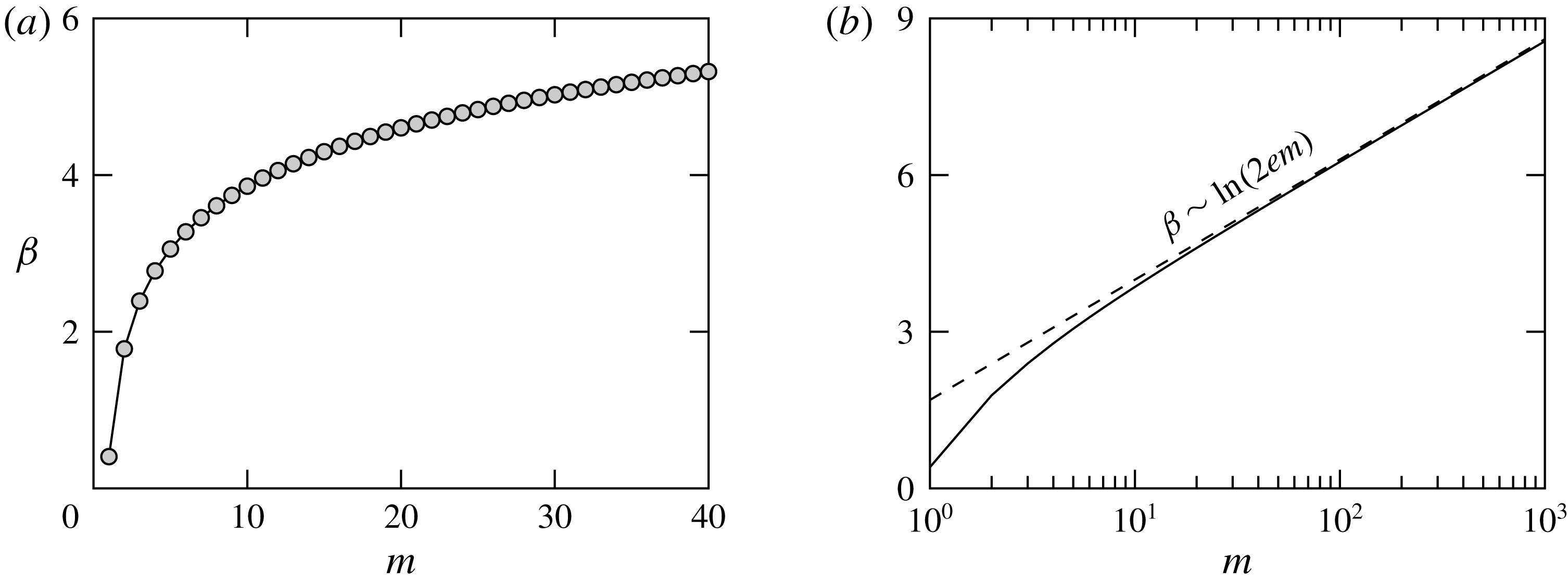
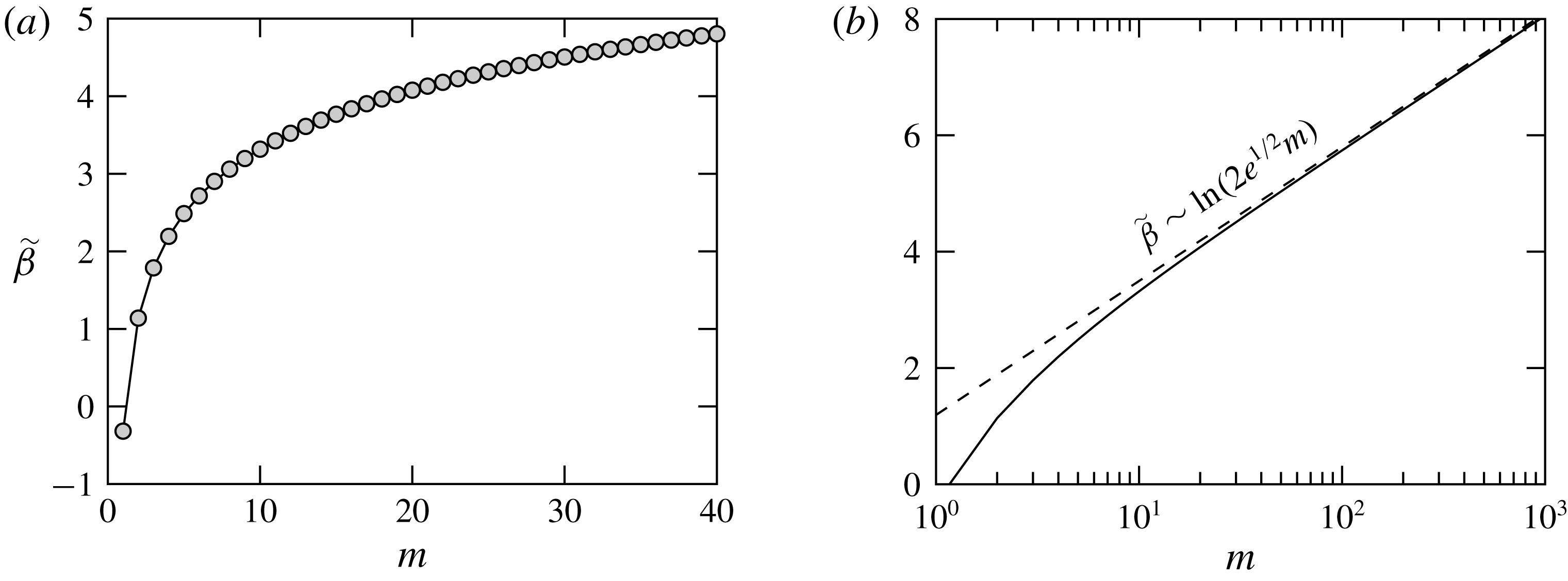
Plot of
 $\unicode[STIX]{x1D6FD}$
as a function of
 $m\geqslant 1$
. (a) The values of
 $\unicode[STIX]{x1D6FD}$
for the first 40 harmonics. (b) Plot on a logarithmic scale for
 $m$
(solid curve), showing also the empirically deduced large-
 $m$
asymptotics of
 $\unicode[STIX]{x1D6FD}$
(dashed curve). In both (a) and (b) the discrete values of
 $\unicode[STIX]{x1D6FD}$
are joined for clarity.

This expression cannot be simplified further and needs to be evaluated numerically. We performed this computation once and the values of
 $\unicode[STIX]{x1D6FD}(m)$
are stored and retrieved in subsequent simulations as necessary. Some implementation details on how
 $\unicode[STIX]{x1D6FD}(m)$
and the associated Gauss hypergeometric function are computed can be found in appendix A. Figure 2 shows the result of this computation, where we see a gradual divergence of
 $\unicode[STIX]{x1D6FD}$
as
 $m\rightarrow \infty$
, which is a manifestation of the breakdown of the theory when
 $m$
becomes sufficiently large. The divergence of
 $\unicode[STIX]{x1D6FD}(m)$
is logarithmic and we see that
 $\unicode[STIX]{x1D6FD}(m)\sim \ln (2\text{e}m)$
fits the numerical data excellently as
 $m\rightarrow \infty$
, noting that this result was obtained empirically. We will return to the behaviour of
 $\unicode[STIX]{x1D6FD}(m)$
for large values of
 $m$
after matching is performed, as this will allow us to set the order of magnitude of
 $M$
, the number of harmonics retained in the truncated Fourier series, (4.1).
Knowing the asymptotics of
 $\unicode[STIX]{x2202}_{r}h_{1,m}$
allows us to obtain the normal derivative of the free surface,
 $\unicode[STIX]{x2202}_{\unicode[STIX]{x1D708}}h_{out}$
as the contact line is approached. We have
 $$\begin{eqnarray}\unicode[STIX]{x2202}_{\unicode[STIX]{x1D708}}h_{out}=\frac{1}{b_{0}}\left(1-\mathop{\sum }_{m=2}^{M}\frac{b_{m}}{b_{0}}\text{e}^{\text{i}m\unicode[STIX]{x1D719}}\right)\unicode[STIX]{x2202}_{r}(h_{0}+h_{1})+\cdots \,,\end{eqnarray}$$
which needs to be evaluated as
 $r\rightarrow 1^{-}$
. We have
 $$\begin{eqnarray}-\unicode[STIX]{x2202}_{\unicode[STIX]{x1D708}}h_{out}\sim \unicode[STIX]{x1D703}+\frac{b_{0}^{6}}{64}\mathop{\sum }_{m=0}^{M}{\dot{b}}_{m}[\ln (1-r)+\unicode[STIX]{x1D6FD}(m)]\text{e}^{\text{i}m\unicode[STIX]{x1D719}}\quad \text{as }r\rightarrow 1^{-},\end{eqnarray}$$
where
 $\unicode[STIX]{x1D703}$
is the (approximate) apparent contact angle
 $$\begin{eqnarray}\unicode[STIX]{x1D703}=\frac{8}{b_{0}^{3}}\left[1+\mathop{\sum }_{m=2}^{M}(1-m)\frac{b_{m}}{b_{0}}\text{e}^{\text{i}m\unicode[STIX]{x1D719}}\right]+\cdots \,.\end{eqnarray}$$
Having obtained the asymptotics of the inner, (4.10), and outer regions, (4.38), the final step of the analysis is to match the two solutions.
4.3 Matching
Just as in the corresponding analysis in two dimensions by Vellingiri et al. (Reference Vellingiri, Savva and Kalliadasis2011), matching is performed with the cubes of the asymptotics of the inner and outer normal derivatives, referring the interested reader to the work of Sibley, Nold & Kalliadasis (Reference Sibley, Nold and Kalliadasis2015a ) which offers a generalisation of how matching can be formally performed for cases when the cubes of the slopes do not match like they do here.
Hence, by considering the third powers of (4.10) and (4.38) we can eliminate the
 $r$
-dependent logarithmic terms, and by requiring that the remaining terms match we find
 $$\begin{eqnarray}\frac{\unicode[STIX]{x1D703}^{3}-\unicode[STIX]{x1D717}_{\ast }^{3}}{3}=\mathop{\sum }_{m=0}^{M}{\dot{b}}_{m}\left[\ln \frac{\text{e}b_{0}\bar{\unicode[STIX]{x1D717}}_{\ast }}{\unicode[STIX]{x1D706}}-\unicode[STIX]{x1D6FD}(m)\right]\text{e}^{\text{i}m\unicode[STIX]{x1D719}},\end{eqnarray}$$
which is reminiscent of the Voinov–Cox–Hocking law and offers an extension of the previous results in two dimensions (Vellingiri et al.
Reference Vellingiri, Savva and Kalliadasis2011) to the three-dimensional setting. It constitutes a simplified problem for the slow motion of a drop, since, as we shall see, the effort required to solve (4.40) is considerably less compared to solving (2.12). Using (4.40), we can write down the evolution equations for
 $b_{m}$
, by collecting the corresponding Fourier coefficients of the left-hand side. Hence, we can write
 $$\begin{eqnarray}{\dot{b}}_{m}=\left(\ln \frac{\text{e}b_{0}\bar{\unicode[STIX]{x1D717}}_{\ast }}{\unicode[STIX]{x1D706}}-\unicode[STIX]{x1D6FD}(m)\right)^{-1}\int _{0}^{2\unicode[STIX]{x03C0}}\frac{\unicode[STIX]{x1D703}^{3}-\unicode[STIX]{x1D717}_{\ast }^{3}}{3\unicode[STIX]{x03C0}}\text{e}^{-\text{i}m\unicode[STIX]{x1D719}}\,\text{d}\unicode[STIX]{x1D719},\end{eqnarray}$$
where the real and imaginary parts of (4.41) give, respectively, ordinary differential equations (ODEs) for the cosine and sine coefficients of the truncated Fourier series in (4.1), except the case when
 $m=1$
which gives ODEs for
 $x_{c}(t)$
and
 $y_{c}(t)$
.
Note that in (4.40) and (4.41) we have not written
 $\unicode[STIX]{x1D703}^{3}$
explicitly in its linearised form for illustration purposes, because the analogy with the two-dimensional geometry is more readily seen this way and also because we will refer to (4.41) later on. We also chose not to assume anything about the strength of the heterogeneities, because, under certain conditions, it is possible to have a nearly circular contact line even when heterogeneities are strong. If we do use (4.39) and retain only the linear terms in
 $b_{m}$
we find
 $$\begin{eqnarray}\displaystyle & \displaystyle {\dot{b}}_{0}=\frac{1}{3}\left(\ln \frac{b_{0}\bar{\unicode[STIX]{x1D717}}_{\ast }}{2\unicode[STIX]{x1D706}\text{e}}\right)^{-1}\left[\frac{512}{b_{0}^{9}}-\frac{1}{2\unicode[STIX]{x03C0}}\int _{0}^{2\unicode[STIX]{x03C0}}\unicode[STIX]{x1D717}_{\ast }^{3}\,\text{d}\unicode[STIX]{x1D719}\right], & \displaystyle\end{eqnarray}$$
 $$\begin{eqnarray}\displaystyle & \displaystyle {\dot{x}}_{c}=-\frac{1}{3\unicode[STIX]{x03C0}}\left(\ln \frac{\text{e}b_{0}\bar{\unicode[STIX]{x1D717}}_{\ast }}{\unicode[STIX]{x1D706}}-\unicode[STIX]{x1D6FD}(1)\right)^{-1}\int _{0}^{2\unicode[STIX]{x03C0}}\unicode[STIX]{x1D717}_{\ast }^{3}\cos \unicode[STIX]{x1D719}\,\text{d}\unicode[STIX]{x1D719}, & \displaystyle\end{eqnarray}$$
 $$\begin{eqnarray}\displaystyle & \displaystyle {\dot{y}}_{c}=-\frac{1}{3\unicode[STIX]{x03C0}}\left(\ln \frac{\text{e}b_{0}\bar{\unicode[STIX]{x1D717}}_{\ast }}{\unicode[STIX]{x1D706}}-\unicode[STIX]{x1D6FD}(1)\right)^{-1}\int _{0}^{2\unicode[STIX]{x03C0}}\unicode[STIX]{x1D717}_{\ast }^{3}\sin \unicode[STIX]{x1D719}\,\text{d}\unicode[STIX]{x1D719}, & \displaystyle\end{eqnarray}$$
 $$\begin{eqnarray}\displaystyle & \displaystyle {\dot{b}}_{m}=\left(\ln \frac{\text{e}b_{0}\bar{\unicode[STIX]{x1D717}}_{\ast }}{\unicode[STIX]{x1D706}}-\unicode[STIX]{x1D6FD}(m)\right)^{-1}\left[\frac{512(1-m)b_{m}}{b_{0}^{10}}-\frac{1}{3\unicode[STIX]{x03C0}}\int _{0}^{2\unicode[STIX]{x03C0}}\unicode[STIX]{x1D717}_{\ast }^{3}\text{e}^{-\text{i}m\unicode[STIX]{x1D719}}\,\text{d}\unicode[STIX]{x1D719}\right],\quad m\geqslant 2.\quad \qquad & \displaystyle\end{eqnarray}$$
 $\unicode[STIX]{x1D717}_{\ast }\equiv 1$
, (4.42a
) reduces to the equation obtained by Hocking (Reference Hocking1983) for axisymmetric droplets in the limit when gravitational effects are negligible, as it should. Also, (4.42b
) and (4.42c
) yield zero net motion, as expected, whereas
 ${\dot{b}}_{m}$
is linear in
 $b_{m}$
giving exponentially decaying solutions for the higher harmonics (see also Greenspan Reference Greenspan1978, Glasner Reference Glasner2005).
The last statement above is valid provided that the first term on the right-hand side of (4.42d
) is always positive for
 $m$
sufficiently large, namely
 $$\begin{eqnarray}\ln \frac{\text{e}b_{0}\bar{\unicode[STIX]{x1D717}}_{\ast }}{\unicode[STIX]{x1D706}}-\unicode[STIX]{x1D6FD}(m)>0.\end{eqnarray}$$
This inequality, however, cannot be true for all values of
 $m$
. The plots in figure 2 show that
 $\unicode[STIX]{x1D6FD}(m)$
grows logarithmically with
 $m$
, which justifies why we considered a truncated Fourier series for
 $a(\unicode[STIX]{x1D719},t)$
; see (4.1). To specify approximately how many terms we must retain, take
 $b_{0}=2$
(the equilibrium angle when
 $\unicode[STIX]{x1D717}_{\ast }\equiv 1$
) and use the empirically obtained asymptotics of
 $\unicode[STIX]{x1D6FD}\sim \ln (2\text{e}m)$
for
 $m\gg 1$
, which gives the criterion
 $M\ll \unicode[STIX]{x1D706}^{-1}$
for the analysis to hold for all terms in (4.1). This, however, is not particularly restrictive for our purposes, because
 $\unicode[STIX]{x1D706}$
is generally a small parameter.
It is important at this stage to contrast our analysis with the work of Greenspan (Reference Greenspan1978) and its extension by Greenspan & McCay (Reference Greenspan and McCay1981). Greenspan (Reference Greenspan1978) used (1.1) and the volume constraint in place of (2.12b
) and (2.12d
). However, enforcing the volume constraint at all times is a result of having zero mass flux along
 $C$
, which, in turn, is also equivalent to the kinematic condition (2.12b
) along
 $C$
(Young Reference Young, Brown and Davis1994). Hence, the condition (1.1) utilised by Greenspan (Reference Greenspan1978) can be viewed as a replacement for our contact angle condition (2.12d
) which become equivalent to each other as
 $k\rightarrow \infty$
. Yet, Greenspan (Reference Greenspan1978) treated (1.1) as a kinematic condition rather than a contact angle condition. This different treatment of (1.1) allows the extraction of evolution equations for the contact line just from the leading-order outer solution, but this type of analysis completely ignores the influence of slip, which is precisely the effect responsible for the contact line motion (see also Hocking Reference Hocking1992, for further comments on this point).
As a result, the slip length does not appear anywhere in the set of equations obtained by Greenspan (Reference Greenspan1978) and Greenspan & McCay (Reference Greenspan and McCay1981). Moreover, it can be seen that the approach to equilibrium is algebraic rather than exponential. Had this condition been utilised properly (see e.g. Hocking Reference Hocking1992, Sibley et al.
Reference Sibley, Nold, Savva and Kalliadasis2015b
) a treatment via matched asymptotics would have been required like here. In the end, however, as Sibley et al. (Reference Sibley, Nold, Savva and Kalliadasis2015b
) have shown, the equations obtained by matching can be made equivalent to each other with a suitable rescaling of
 $\unicode[STIX]{x1D706}$
. It is noteworthy that Hocking (Reference Hocking1992) criticised conditions of the form (1.1) arguing against their usefulness given that the dynamics can be formally mapped to the dynamics arising from using (2.12d
), which does not depend on additional material constants, such as
 $k$
in (1.1).
Apart from these key differences in the methodology, we should emphasise that our approach is general and can deal with droplets undergoing any type of motion. In contrast, Greenspan (Reference Greenspan1978) and Greenspan & McCay (Reference Greenspan and McCay1981) considered separately the cases where the local contact angle exhibits linear spatial variations and when the droplet does not move from its original position so that the contact line can be described in a fixed polar coordinate system at all times. In contrast, (4.40) can be used to treat both cases just as easily.
5 Numerical methods
In the following sections we will explore numerical solutions to both (2.12) and (4.40) in various settings, in order to assess how well the lower-dimensional system approximates the full system. In what follows, the full problem refers to the PDEs subject to the appropriate initial and boundary conditions, (2.12), whereas the reduced problem refers to the system of ODEs obtained from matching, (4.40). We also propose a hybrid method which utilises the results of the analysis and the boundary integral formalism, borrowing ideas from Glasner (Reference Glasner2005).
5.1 Reduced problem
The reduced problem, (4.40) and its linearised version (4.42) is generally a non-stiff system of ODEs, where we have explicit expressions for each harmonic, but coupling of each component can arise through the computation of
 $\bar{\unicode[STIX]{x1D717}}_{\ast }$
and the harmonics of
 $\unicode[STIX]{x1D717}_{\ast }^{3}$
. In general, we use
 $M=150$
, resulting in 301 unknowns (one axisymmetric component and 150 Fourier cosine and 150 sine modes). The input variables at each time step, namely
 $a_{m}(t)$
,
 $x_{c}(t)$
and
 $y_{c}(t)$
, are used to construct the contact line using the inverse fast Fourier transform, which allows us to obtain
 $\unicode[STIX]{x1D717}_{\ast }^{3}$
. Then
 $\unicode[STIX]{x1D717}_{\ast }^{3}$
is decomposed into its Fourier modes using the fast Fourier transform, which are then used in either (4.40) or (4.42) to extract the values for
 ${\dot{b}}_{m}$
and perform the time stepping using the routine ode15s in MATLAB. This is a rather straightforward implementation and a typical simulation takes about one minute or less on a standard personal computer.
5.2 Full problem
The full problem requires significantly more effort, both in terms of implementation and actual computing time, as it amounts to solving a set of coupled stiff PDEs for
 $h(r,\unicode[STIX]{x1D719},t)$
and
 $a(\unicode[STIX]{x1D719},t)$
as well as a set of ODEs for the coordinates of the centroid,
 $(x_{c}(t),y_{c}(t))$
. The numerical issues due to stiffness worsen as
 $\unicode[STIX]{x1D706}\rightarrow 0$
, because the boundary layers in
 $\unicode[STIX]{x2202}_{\unicode[STIX]{x1D708}}h$
become narrower, thus requiring more mesh points near the contact line to be resolved.
Such difficulties need to be overcome in order to perform the computations accurately and efficiently, and to properly compare the results of our analysis with the predictions of the full problem. Here we opted for the pseudospectral collocation method, which has been successfully used in the past by the present authors to deal with contact line problems in two dimensions (see e.g. Savva & Kalliadasis Reference Savva and Kalliadasis2009, Reference Savva and Kalliadasis2011, Reference Savva and Kalliadasis2012, Reference Savva and Kalliadasis2013, Reference Savva and Kalliadasis2014). An attractive feature of this method is that it naturally clusters collocation points near the contact line, which allows us to capture boundary-layer dynamics with comparatively fewer collocation nodes as opposed to, say, a finite difference scheme based on a uniform grid. Although giving all the fine details of our numerical method is beyond the scope of this work, its basic principles are briefly outlined in appendix B.
5.3 Hybrid approach
The hybrid approach provides an attractive compromise between the speed of solving the low-order, reduced model, (4.40), and the accuracy of the full problem, (2.12). It is based on the observation that the apparent contact angle used in (4.40) is only approximately provided from low-order corrections about a circular contact line, obtained by solving Laplace’s equation by a truncated perturbation series; see (4.14).
In essence, the reduced model uses as input the contact line harmonics, from which the harmonics of the apparent contact angle are obtained by solving Laplace’s equation approximately. From the apparent contact angle, the reduced model then gives the rates of change of each harmonic of the contact line. Hence, as we shall see in the next section, the equilibrium obtained in the long-time limit by solving the reduced problem can often be different from that obtained by solving the full problem. This shortcoming of the reduced model can be remedied by solving numerically Laplace’s equation, thus obtaining improved approximations for the apparent contact angle at each time step.
The most appropriate method to solve Laplace’s equation in this setting is arguably the boundary integral method, as it outputs directly the apparent contact angle. This requires significantly less computational effort as opposed to traditional discretisation schemes, which determine the solution everywhere in the domain. This approach is similar to the work of Glasner (Reference Glasner2005), apart from the evolution of the contact line, which was computed by specifying the form of the normal velocity of the contact line as
 $\boldsymbol{v}\boldsymbol{\cdot }\unicode[STIX]{x1D742}=\unicode[STIX]{x1D703}^{3}-\unicode[STIX]{x1D717}_{\ast }^{3}$
. A notable difference between our work and Glasner’s is that Glasner parametrised the contact line with respect to the arc length, unlike here where the parametrisation is done with respect to the polar angle. Glasner’s parametrisation allows the investigation of cases where the contact line cannot be described by a one-to-one function in polar coordinates. However, we do not require such flexibility since the presented asymptotic theory assumes weak contact line deformations.
Although the problem set-up is nearly identical to the work of Glasner (Reference Glasner2005), for the sake of completeness we reproduce its main results adapted to our notation and providing more details on the implementation in appendix C. Thus, for a given contact line shape, we wish to solve numerically the leading-order outer problem, (4.16). In this quasi-static setting, time is frozen, so
 $q(t)$
needs to be determined from the volume constraint, (3.14), cast in the form
 $$\begin{eqnarray}\int _{\unicode[STIX]{x1D6FA}(t)}h_{0}(\boldsymbol{x},t)\,\text{d}\boldsymbol{x}=V,\end{eqnarray}$$
where
 $\unicode[STIX]{x1D6FA}(t)$
denotes the wet region of the substrate and
 $\boldsymbol{x}=(x-x_{c},y-y_{c})$
. Central to the boundary integral formulation is the free-space Green’s function,
 $$\begin{eqnarray}G(\boldsymbol{x},\boldsymbol{x}_{0})=-\frac{1}{2\unicode[STIX]{x03C0}}\ln |\boldsymbol{x}-\boldsymbol{x}_{0}|,\end{eqnarray}$$
which is the radially symmetric solution to
 $$\begin{eqnarray}-\unicode[STIX]{x1D6FB}^{2}G(\boldsymbol{x},\boldsymbol{x}_{0})=\unicode[STIX]{x1D6FF}(\boldsymbol{x}-\boldsymbol{x}_{0})\quad \text{for }\boldsymbol{x},\,\boldsymbol{x}_{0}\in \mathbb{R}^{2},\end{eqnarray}$$
where
 $\unicode[STIX]{x1D6FF}$
denotes the Dirac delta function. To proceed, define
 $$\begin{eqnarray}w(\boldsymbol{x},t)=\frac{h_{0}(\boldsymbol{x},t)}{q(t)}+\frac{|\boldsymbol{x}|^{2}}{4},\end{eqnarray}$$
so that (4.16a
) and (4.16b
) prescribe the following problem for
 $w(\boldsymbol{x},t)$
:
 $$\begin{eqnarray}\displaystyle & \displaystyle \unicode[STIX]{x1D6FB}^{2}w(\boldsymbol{x},t)=0\quad \text{for }\boldsymbol{x}\in \unicode[STIX]{x1D6FA}(t), & \displaystyle\end{eqnarray}$$
 $$\begin{eqnarray}\displaystyle & \displaystyle w(\boldsymbol{x},t)=\frac{|\boldsymbol{x}|^{2}}{4}\quad \text{for }\boldsymbol{x}\in C(t). & \displaystyle\end{eqnarray}$$
 $h_{0}$
. Multiplying (5.5a
) by (5.2) and making use of Green’s second integral identity gives, after some term rearrangement, the following boundary integral equation:
 $$\begin{eqnarray}\int _{C(t)}G(\boldsymbol{x},\boldsymbol{x}_{0})\unicode[STIX]{x2202}_{\unicode[STIX]{x1D708}}w(\boldsymbol{x},t)\,\text{d}s(\boldsymbol{x})=\frac{|\boldsymbol{x}_{0}|^{2}}{8}+\frac{1}{4}\int _{C(t)}|\boldsymbol{x}|^{2}\unicode[STIX]{x2202}_{\unicode[STIX]{x1D708}}G(\boldsymbol{x},\boldsymbol{x}_{0})\,\text{d}s(\boldsymbol{x}),\end{eqnarray}$$
where
 $\unicode[STIX]{x2202}_{\unicode[STIX]{x1D708}}w$
and
 $\unicode[STIX]{x2202}_{\unicode[STIX]{x1D708}}G$
denote the normal derivatives of
 $w$
and
 $G$
, respectively, and
 $\boldsymbol{x}_{0}$
is a point on the contact line,
 $C(t)$
. Equation (5.6) can be solved for the unknown values of
 $\unicode[STIX]{x2202}_{\unicode[STIX]{x1D708}}w$
along
 $C(t)$
, from which we may determine
 $q(t)$
and then specify the apparent contact angle
 $\unicode[STIX]{x1D703}=-\unicode[STIX]{x2202}_{\unicode[STIX]{x1D708}}h_{0}|_{C(t)}$
via (5.4), namely
 $$\begin{eqnarray}\unicode[STIX]{x1D703}(\boldsymbol{x},t)=-\unicode[STIX]{x2202}_{\unicode[STIX]{x1D708}}h_{0}(\boldsymbol{x},t)=q(t)\left[\frac{\boldsymbol{x}\boldsymbol{\cdot }\unicode[STIX]{x1D742}}{2}-\unicode[STIX]{x2202}_{\unicode[STIX]{x1D708}}w(\boldsymbol{x},t)\right],\quad \boldsymbol{x}\in C(t).\end{eqnarray}$$
Thus, to determine
 $q(t)$
, we follow Glasner (Reference Glasner2005) and consider (5.1) as
 $$\begin{eqnarray}V=\frac{1}{4}\int _{\unicode[STIX]{x1D6FA}(t)}h_{0}(\boldsymbol{x},t)\unicode[STIX]{x1D6FB}^{2}|\boldsymbol{x}|^{2}\,\text{d}\boldsymbol{x}.\end{eqnarray}$$
Then, utilising Green’s second integral identity, followed by the identity
 $\unicode[STIX]{x1D735}\boldsymbol{\cdot }(|\boldsymbol{x}|^{2}\boldsymbol{x})=4|\boldsymbol{x}|^{2}$
, (5.7) and the divergence theorem, (5.8) becomes
 $$\begin{eqnarray}V=\frac{q(t)}{4}\int _{C(t)}|\boldsymbol{x}|^{2}\left(\frac{\boldsymbol{x}\boldsymbol{\cdot }\unicode[STIX]{x1D742}}{4}-\unicode[STIX]{x2202}_{\unicode[STIX]{x1D708}}w\right)\,\text{d}s(\boldsymbol{x}),\end{eqnarray}$$
which allows us to compute
 $q(t)$
once
 $\unicode[STIX]{x2202}_{\unicode[STIX]{x1D708}}w$
is known on
 $C(t)$
. Equation (5.9) is equivalent to equation (11) in Glasner (Reference Glasner2005), noting that it contains a typo in the first term inside the integral, which should read
 $|\boldsymbol{x}|^{2}\boldsymbol{x}\boldsymbol{\cdot }\unicode[STIX]{x1D742}/16$
instead of
 $|\boldsymbol{x}|^{2}\boldsymbol{x}/16$
. Summarising, the boundary integral formulation for obtaining the apparent contact angle involves solving an integral equation, (5.6), which results in a dense linear system for
 $\unicode[STIX]{x2202}_{\unicode[STIX]{x1D708}}w$
, computing
 $q(t)$
from (5.9) and
 $\unicode[STIX]{x1D703}(\boldsymbol{x})$
from (5.7). Further details about how these computations can be performed are given in appendix C. The hybrid analytical–numerical approach is closed by using the outcome of this calculation,
 $\unicode[STIX]{x1D703}(\boldsymbol{x})$
, in conjunction with the rates of change of the harmonics of the contact line, (4.40). The evolution of the contact line is then computed analogously to the reduced system. Some comparisons with Lacey’s leading-order asymptotic result are also offered in the present study, by solving (3.7), (3.12) and (3.13) with
 $W=(\unicode[STIX]{x1D717}_{\ast }^{3}-\unicode[STIX]{x1D703}^{3})\sqrt{a^{2}+(\unicode[STIX]{x2202}_{\unicode[STIX]{x1D719}}a)^{2}}/(3\ln \unicode[STIX]{x1D706})$
.
6 Results
In this section, we describe a number of test cases to examine the level of agreement of our analysis with the governing PDE, offering, where appropriate, comparisons with the full, reduced, hybrid and Lacey’s model together with the appropriate commentary. Unless specified otherwise, in most computations we kept
 $\unicode[STIX]{x1D706}=10^{-4}$
. Note also that in many of the tests presented in the following sections the local contact angles as prescribed through
 $\unicode[STIX]{x1D717}(x,y)$
are generally sharply varying so that the assumption of a nearly circular contact line is not really applicable. However, this is arguably the best way to assess how well the hybrid approach performs in those cases given that it is based on a theory developed for nearly circular contact lines. In all cases presented, with the exception of the linear wettability gradients, the computations were terminated when the droplet was deemed to be sufficiently close to its equilibrium state.
Snapshots of the rightward droplet motion on linear wettability gradients at times
 $t=0,$
200, 400, 600, 800 and 1000 with
 $a(\unicode[STIX]{x1D719},0)=1$
for (a)
 $\unicode[STIX]{x1D717}(x,y)=1-0.01x$
and (b)
 $\unicode[STIX]{x1D717}(x,y)=1-0.1x$
. (c) Evolution of the
 $x$
-coordinate of the centroid for each of the calculations in (a) and (b). Solid and dashed curves correspond to solutions of the full and reduced problems, (2.12) and (4.42), respectively. The dotted curves in (c) show the respective estimates found from (6.2), whereas the grey curves show the results of the hybrid method based on Lacey’s leading-order asymptotics, (1.2).

6.1 Linear wettability gradients
In the first set of examples, we consider substrates with linear wettability gradients, so that the local contact angle is prescribed according to
 $$\begin{eqnarray}\unicode[STIX]{x1D717}(x,y)=1-\unicode[STIX]{x1D6FC}x,\end{eqnarray}$$
where
 $0<\unicode[STIX]{x1D6FC}\ll 1$
and we naturally restrict the values of
 $x$
or the time at which the computation is terminated, so that
 $\unicode[STIX]{x1D717}$
is both non-negative and at most
 $O(1)$
. In this case we can obtain an analytical estimate for the velocity of the centroid, which is valid for early times. The starting point to deduce this estimate is to assume that if the contact line is axisymmetric initially it will remain so at least during the early stages of the motion. Based on the discussion surrounding our linearised equations, (4.42), even if the contact line is not perfectly circular initially, the higher harmonics will tend to die out rather quickly. Assuming further that the axisymmetric component of the contact line is close to the equilibrium radius on a homogeneous substrate, i.e.
 $a_{0}=2+O(\unicode[STIX]{x1D6FC})$
, allows us to deduce the initial speed of the droplet at which it translates rightward, towards the more wettable regions of the substrate. We find
 $$\begin{eqnarray}{\dot{x}}_{c}=2\unicode[STIX]{x1D6FC}\left(\ln \frac{2\text{e}}{\unicode[STIX]{x1D706}}-\unicode[STIX]{x1D6FD}(1)\right)^{-1}\approx \frac{2\unicode[STIX]{x1D6FC}}{1.2873+\ln \unicode[STIX]{x1D706}^{-1}}.\end{eqnarray}$$
It should be noted here that comparing the analysis undertaken by Pismen (Reference Pismen2006) in this setting differs from (6.2), without the constant term in its denominator, by a factor of two. This difference can be traced to equation (10) in that paper being incorrectly assumed to hold. Two sample calculations using (6.1) are presented in figure 3, where we note the excellent agreement of the reduced problem with the full problem. In figure 3(c) we show that when
 $\unicode[STIX]{x1D6FC}=0.01$
the contact line remains nearly circular and the droplet translates at a nearly constant speed with excellent agreement between (6.2) and the numerics. For
 $\unicode[STIX]{x1D6FC}=0.1$
(6.2) is an acceptable approximation only for early times; the contact line is no longer circular and the second harmonic
 $a_{2}$
becomes appreciable (see figure 3
b). Our reduced model is able to capture this behaviour rather well, unlike the analysis by Greenspan (Reference Greenspan1978) which is based on the assumption that the contact line remains circular when there are linear wettability gradients. We see also that the agreement is less favourable with the hybrid method based on Lacey’s result, (1.2), unlike the hybrid method based on (4.40), which is indistinguishable from the full problem (not shown in figure 3 for clarity).
6.2 Stripe-patterned substrates
Snapshots of droplet profiles during spreading on chemically stripe-patterned surfaces with
 $\unicode[STIX]{x1D706}=10^{-4}$
at different times. (a) Profiles at times
 $t=0$
, 0.5, 5 and 50 when
 $\unicode[STIX]{x1D717}(x,y)=1+0.3\tanh [2\sin (2\unicode[STIX]{x03C0}x)]$
and
 $a(\unicode[STIX]{x1D719},0)=1.5+0.1\sin (3\unicode[STIX]{x1D719})-0.1\sin (6\unicode[STIX]{x1D719})$
. (b) Profiles at times
 $t=0$
, 0.05, 0.25 and 5 when
 $\unicode[STIX]{x1D717}(x,y)=2+\tanh [5\sin (5\unicode[STIX]{x03C0}x)]$
and
 $a(\unicode[STIX]{x1D719},0)=1$
. In (a) and (b) solid, dashed and dotted curves correspond to solutions to the full, reduced and hybrid problems, respectively. The substrate is coloured in shades of grey according to the minimum (dark grey) and maximum (white) values of
 $\unicode[STIX]{x1D717}$
.

As mentioned in § 1, stripe-patterned substrates have been studied extensively in experiments. Spreading typically occurs along the stripes, giving rise to elongated droplet shapes. The degree of elongation depends crucially on the wettability contrast between the stripes, as well as on the width of the stripes. In figure 4 we explore two such cases. In the first case, figure 4(a), we start off from a non-circular contact line shape and within
 $t=0.5$
it becomes nearly circular. The droplet spreads more along the
 $y$
-direction, as expected, and the contact line ultimately becomes pinned along the boundary separating two stripes, having shifted slightly to the right to lie symmetrically with respect to the substrate features. In the second case, figure 4(b), the substrate has a higher wettability contrast and narrower stripes. We notice significant distortions of the contact line which become more pronounced as the droplet trends to equilibrium. In this case, the contact line becomes both more elongated and more distorted. These calculations demonstrate excellent agreement of the reduced and full problems at the onset. However, as the contact line becomes more distorted and increasingly non-circular, the agreement deteriorates; see e.g. the profile shown in figure 4(b) at
 $t=5$
. However, the hybrid approach tends to perform excellently throughout.
Let us note that our numerical methods failed in a number of tests to resolve receding contact lines on striped surfaces with sharp wettability contrasts. In these cases, the contact line tends to develop finger-like shapes as it recedes and our spatial discretisation scheme under-resolves such contact line profiles. Since such contact line shapes are far from being circular, we did not deem it necessary to pursue such cases further.
6.3 Random heterogeneities
Spreading on a substrate with random wettability patches with
 $\unicode[STIX]{x1D706}=10^{-4}$
,
 $a(\unicode[STIX]{x1D719},0)=1+0.05\sin (3\unicode[STIX]{x1D719})-0.05\sin (6\unicode[STIX]{x1D719})$
and
 $x_{c}(0)=y_{c}(0)=0$
(see main text for a description of how the substrate was generated). (a) Contact line profiles when
 $t=0$
, 0.02, 0.3, 1, 3 and 30. (b) Overlays of contact line profiles from the solution to the full problem, shown at a zoomed-in portion of the substrate. Refer to figure 4 for a description of the various curves and substrate shading.

The next example concerns a substrate with
 $\unicode[STIX]{x1D717}(x,y)$
described by a superposition of localised random, nearly circular features according to
 $$\begin{eqnarray}\unicode[STIX]{x1D717}(x,y)=1+\mathop{\sum }_{j=1}^{n}\unicode[STIX]{x1D702}\left(\sqrt{(x-\bar{x}_{j})^{2}+(y-\bar{y}_{j})^{2}},\unicode[STIX]{x1D6FE}_{j},d_{j},\unicode[STIX]{x1D705}\right),\end{eqnarray}$$
where
 $n$
is the number of the features considered,
 $(\bar{x}_{j},\bar{y}_{j})$
denote the centres of each localised feature and
 $\unicode[STIX]{x1D702}$
is a smooth, step-like function given by
 $$\begin{eqnarray}\unicode[STIX]{x1D702}(x,\unicode[STIX]{x1D6FE},d,\unicode[STIX]{x1D705})=\frac{\unicode[STIX]{x1D6FE}}{2}[\tanh (\unicode[STIX]{x1D705}(x+d))-\tanh (\unicode[STIX]{x1D705}(x-d))],\end{eqnarray}$$
where
 $\unicode[STIX]{x1D6FE}$
is the amplitude,
 $\unicode[STIX]{x1D705}\gg 1$
is a measure of the sharpness of the step and
 $d$
roughly corresponds to its half-width. Here we fixed
 $n=200$
,
 $(\bar{x}_{j},\bar{y}_{j})$
are uniformly randomly distributed in the square
 $(-2.5,2.5)\times (-2.5,2.5)$
,
 $\unicode[STIX]{x1D6FE}_{j}$
are uniformly randomly distributed in the interval
 $(-0.2,1.2)$
,
 $d_{j}$
are uniformly randomly distributed in the interval
 $(0,0.2)$
and
 $\unicode[STIX]{x1D705}=20$
.
The result of this computation is shown in figure 5. Evidently, during the early stages the contact line remains nearly circular, advancing undisturbed by the presence of the defects (figure 5 a). However, as the droplet approaches equilibrium, the contact line undergoes appreciable deformations due to the localised pinning occurring near defects. This pinning is weaker and temporary at first and the contact line manages to overcome the wettability barriers it encounters as it advances (see figure 5 b). Ultimately, the contact line reaches equilibrium when the curvature pressure which drives the motion is no longer strong enough to push the contact line past the defects, thus ultimately trapping the contact line.
As in all previous cases, the agreement of the hybrid and full problems is excellent. However, the reduced problem fails to capture the stick–slip event which occurs near (1.2,1.2) (see figure 5 b) and the contact line reaches a markedly different equilibrium in the long-time limit (see figure 5 a). Although this has not been commonly observed in the tests we performed, the example is presented here to show that the neglected terms in the analysis may sometimes cause the droplet to behave differently from what the full problem predicts. Such differences may equally arise due to discretisation errors in the full problem. Note that a similar observation was also made in the two-dimensional setting, particularly when there are many local droplet equilibria (see Savva & Kalliadasis Reference Savva and Kalliadasis2011).
6.4 Complex patterns and higher-order effects
Spreading on the dartboard pattern given by (6.5) with
 $\unicode[STIX]{x1D706}=10^{-4}$
,
 $x_{c}(0)=0.5$
,
 $y_{c}(0)=0$
and
 $a(\unicode[STIX]{x1D719},0)=1$
. (a) Snapshots of the contact line when
 $t=0$
, 0.05, 0.5, 5 and 40. Refer to figure 4 for a description of the various curves and substrate shading. (b) The relative change in the values of
 $a(\unicode[STIX]{x1D719},t)$
obtained from the full problem compared to the reduced problem (dashed curve) and the hybrid approach (solid curve) when
 $t=30$
.

We continue with two further illustrative examples involving more complex patterns. The first example is that of a dartboard pattern defined by the equation
 $$\begin{eqnarray}\unicode[STIX]{x1D717}(x,y)=\frac{6}{5}+\frac{4}{5}\tanh \left[10\sin \left(6\arctan \frac{y}{x}\right)\right]\tanh [10\sin (\unicode[STIX]{x03C0}\sqrt{x^{2}+y^{2}})],\end{eqnarray}$$
where the values of
 $\unicode[STIX]{x1D717}$
vary approximately between 0.4 and 2. The results of the calculations using (6.5) are shown in figure 6 and demonstrate once more the excellent agreement of the hybrid approach with the full problem, where at all times the predictions of the contact line locations differ by less than 1 % (see figure 6
b). In contrast, the reduced problem exhibits excellent agreement at the early stages of the dynamics, but as the droplet approaches equilibrium we see differences of up to 10 % from the full problem (see also the profiles in figure 6
a when
 $t=5$
and 40). This is to be expected given that the droplet develops pronounced protrusions as the contact line fronts invade the more wettable regions of the substrate, so the assumption that the contact line is nearly circular ceases to be valid.
Snapshots of the contact line for a droplet moving on a substrate with
 $\unicode[STIX]{x1D717}(x,y)$
given by (6.6),
 $\unicode[STIX]{x1D706}=10^{-3}$
,
 $x_{c}(0)=-3$
,
 $y_{c}(0)=2.5$
and
 $a(\unicode[STIX]{x1D719},0)=1$
. The droplet migrates from the less hydrophilic region (top) to the more hydrophilic region (bottom). The substrate is shaded as in figure 4. Snapshots correspond to times
 $t=0$
, 20, 60, 100, 140, 200 and 400. The white curve tracks the motion of the centroid of the contact area; white circles show the centroid locations corresponding to each of the snapshot shown. The solid curves correspond to the solution to the full problem. The dashed curves in (a) and (b) correspond, respectively, to the solutions to the hybrid problems using (4.40) and Lacey’s result, (1.2).

The second and final example where we compare the calculations of the full problem and the predictions of our theory concerns a more contrived setting where we superimpose a chequerboard pattern and a chemical gradient inducing a directional motion towards the more hydrophilic regions of the substrate. More specifically, the spatial variations of the contact angle are prescribed according to
 $$\begin{eqnarray}\unicode[STIX]{x1D717}(x,y)=\frac{11}{5}+\frac{1}{\unicode[STIX]{x03C0}}\left\{1-\frac{1}{4}g_{1}(x,y)\right\}g_{2}(x,y)\arctan \frac{y}{x}+\frac{1}{3}g_{1}(x,y),\end{eqnarray}$$
where the inverse tangent provides the gradient,
 $$\begin{eqnarray}g_{1}(x,y)=\{1-\tanh [20(y+1)]\tanh [20(y-1)]\}\{1-\tanh [20(x-1)]\}\end{eqnarray}$$
is roughly equal to 4 when
 $|y|\leqslant 1$
and
 $x\leqslant 1$
and is used to mask the region where the inverse tangent is multivalued and
 $$\begin{eqnarray}g_{2}(x,y)=1+\frac{3}{10}\tanh [3\cos (\unicode[STIX]{x03C0}x)]\tanh [3\sin (\unicode[STIX]{x03C0}y)]\end{eqnarray}$$
provides a chequerboard pattern. For this choice of
 $\unicode[STIX]{x1D717}$
, the contact angle is approximately 3.5 when
 $|y|\leqslant 1$
and
 $x\leqslant 1$
, so that it poses essentially a wettability barrier, which the droplet avoids. The minimum contact angle is approximately unity.
The reason for this choice is basically to test our theory in the case when the droplet undergoes a long excursion from its original position. Here we set
 $\unicode[STIX]{x1D706}=10^{-3}$
and solved for
 $0\leqslant t\leqslant 400$
. Snapshots of the contact line are shown at different times in figure 7, where we see how the droplet evolves as it seeks an equilibrium towards the more hydrophilic region of the substrate. Interestingly this is not the only equilibrium, noting that there can also exist equilibria in the less hydrophilic region, near the initial droplet location (not shown here).
Although the contact line remains nearly circular at all times, the discretisation in the azimuthal direction requires a dense mesh because the value of the contact angle along the contact line exhibits sharp variations due to the chequerboard pattern. However, for the first time we see appreciable deviations from the predictions of the hybrid and full problems (see figure 7 a). The reduced problem gives very similar results to the hybrid one, but the comparison of the full problem with the leading-order asymptotic result from Lacey, (1.2), is rather poor (see figure 7 b), illustrating the importance of going beyond the leading-order terms in the asymptotic analysis.
Plot of
 $\tilde{\unicode[STIX]{x1D6FD}}$
as a function of
 $m\geqslant 1$
. (a) The values of
 $\tilde{\unicode[STIX]{x1D6FD}}$
for the first 40 harmonics. (b) Plot on a logarithmic scale for
 $m$
(solid curve), showing also the empirically deduced large-
 $m$
asymptotics of
 $\tilde{\unicode[STIX]{x1D6FD}}$
(dashed curve). In both (a) and (b) the discrete values of
 $\tilde{\unicode[STIX]{x1D6FD}}$
were joined for clarity.

The discrepancy, which becomes more prominent at intermediate times, can be attributed, at least in part, to the logarithmically singular terms we omitted in our analysis; see e.g. the discussion surrounding (4.7). To include these terms a more elaborate analysis is required. In such a case, using (4.7) in (4.6) and retaining the appropriate terms yields
 $$\begin{eqnarray}\displaystyle & & \displaystyle -(\unicode[STIX]{x2202}_{\unicode[STIX]{x1D708}}h_{in})^{3}\sim \unicode[STIX]{x1D717}_{\ast }^{3}+3\ln \left(\text{e}b_{0}\bar{\unicode[STIX]{x1D717}}_{\ast }\frac{1-r}{\unicode[STIX]{x1D706}}\right)\left\{{\dot{b}}_{0}+\left({\dot{b}}_{1}-\frac{b_{2}}{b_{0}}{\dot{b}}_{1}^{\ast }\right)\text{e}^{\text{i}\unicode[STIX]{x1D719}}+\left({\dot{b}}_{2}-\frac{3b_{3}}{2b_{0}}{\dot{b}}_{1}^{\ast }\right)\text{e}^{2\text{i}\unicode[STIX]{x1D719}}\right.\nonumber\\ \displaystyle & & \displaystyle \quad +\left.\mathop{\sum }_{m=3}^{M}\left({\dot{b}}_{m}+\frac{(m-1)b_{m-1}}{2b_{0}}{\dot{b}}_{1}-\frac{(m+1)b_{m+1}}{2b_{0}}{\dot{b}}_{1}^{\ast }\right)\text{e}^{\text{i}m\unicode[STIX]{x1D719}}\right\}+\cdots \,,\end{eqnarray}$$
as
 $b_{0}(1-r)/\unicode[STIX]{x1D706}\rightarrow \infty$
. By looking at the outer-region dynamics, we see that (4.15) must include the contributions coming from such terms, namely
 $$\begin{eqnarray}\displaystyle h_{1}(r,\unicode[STIX]{x1D719},t) & = & \displaystyle \mathop{\sum }_{m=0}^{M}{\dot{b}}_{m}h_{1,m}(r,b_{0})\text{e}^{\text{i}m\unicode[STIX]{x1D719}}-\frac{b_{2}}{b_{0}}{\dot{b}}_{1}^{\ast }\tilde{h}_{1,1}(r,b_{0})\text{e}^{\text{i}\unicode[STIX]{x1D719}}-\frac{3b_{3}}{2b_{0}}{\dot{b}}_{1}^{\ast }\tilde{h}_{1,2}(r,b_{0})\text{e}^{2\text{i}\unicode[STIX]{x1D719}}\nonumber\\ \displaystyle & & \displaystyle +\,\mathop{\sum }_{m=3}^{M}\left(\frac{(m-1)b_{m-1}}{2b_{0}}{\dot{b}}_{1}-\frac{(m+1)b_{m+1}}{2b_{0}}{\dot{b}}_{1}^{\ast }\right)\tilde{h}_{1,m}(r,b_{0})\text{e}^{\text{i}m\unicode[STIX]{x1D719}}+\cdots \,,\qquad\end{eqnarray}$$
where
 $\tilde{h}_{1,m}$
with
 $m\geqslant 1$
correspond to the new terms. Just like the analysis of the asymptotics of
 $h_{1,m}$
, we expect that
 $$\begin{eqnarray}-\unicode[STIX]{x2202}_{r}\tilde{h}_{1,m}\sim \frac{b_{0}^{7}}{64}[\ln (1-r)+\tilde{\unicode[STIX]{x1D6FD}}(m)]+\cdots \quad \text{as }r\rightarrow 1^{-},\end{eqnarray}$$
where
 $\tilde{\unicode[STIX]{x1D6FD}}(m)$
is a function of
 $m$
that needs to be determined. By following a series of steps which are similar to those required to obtain
 $\unicode[STIX]{x1D6FD}$
we find
 $$\begin{eqnarray}\tilde{\unicode[STIX]{x1D6FD}}(m)=\int _{0}^{1}\frac{1}{1-r}[1-r^{m+1}\tilde{P}_{m}(r)]\,\text{d}r,\end{eqnarray}$$
where
 $\tilde{P}_{m}(r)$
satisfies the differential equation
 $$\begin{eqnarray}8r^{2}+r\frac{\text{d}}{\text{d}r}\left[r(1-r^{2})^{3}\frac{\text{d}}{\text{d}r}\left(\frac{\tilde{P}_{m}}{1-r}\right)\right]-m^{2}(1-r^{2})^{3}\frac{\tilde{P}_{m}}{1-r}=0,\end{eqnarray}$$
with conditions
 $\tilde{P}_{m}(0)=0$
and
 $\tilde{P}_{m}(1)=1$
. To obtain
 $\tilde{\unicode[STIX]{x1D6FD}}(m)$
we utilise the same techniques which were used to get
 $\unicode[STIX]{x1D6FD}(m)$
(see appendix A). As figure 8 shows, the behaviour of
 $\tilde{\unicode[STIX]{x1D6FD}}(m)$
as
 $m$
varies is rather similar to that of
 $\unicode[STIX]{x1D6FD}(m)$
.
Therefore, the behaviour of the cube of the normal derivative of the solution in the outer region as
 $r\rightarrow 1^{-}$
is given by
 $$\begin{eqnarray}\displaystyle & & \displaystyle -(\unicode[STIX]{x2202}_{\unicode[STIX]{x1D708}}h_{out})^{3}\sim \unicode[STIX]{x1D703}^{3}+3\mathop{\sum }_{m=0}^{M}{\dot{b}}_{m}[\ln (1-r)+\unicode[STIX]{x1D6FD}(m)]\text{e}^{\text{i}m\unicode[STIX]{x1D719}}\nonumber\\ \displaystyle & & \displaystyle \quad -\,\frac{3b_{2}}{b_{0}}{\dot{b}}_{1}^{\ast }[\ln (1-r)+\tilde{\unicode[STIX]{x1D6FD}}(1)]\text{e}^{\text{i}\unicode[STIX]{x1D719}}-\frac{9b_{3}}{2b_{0}}{\dot{b}}_{1}^{\ast }[\ln (1-r)+\tilde{\unicode[STIX]{x1D6FD}}(2)]\text{e}^{2\text{i}\unicode[STIX]{x1D719}}\nonumber\\ \displaystyle & & \displaystyle \quad +\,\frac{3}{2b_{0}}\mathop{\sum }_{m=3}^{M}[(m-1)b_{m-1}{\dot{b}}_{1}-(m+1)b_{m+1}{\dot{b}}_{1}^{\ast }][\ln (1-r)+\tilde{\unicode[STIX]{x1D6FD}}(m)]\text{e}^{\text{i}m\unicode[STIX]{x1D719}},\end{eqnarray}$$
which is matched with (6.9) to yield the following system of differential equations,
 $$\begin{eqnarray}\displaystyle & \displaystyle {\dot{b}}_{0}=\frac{g_{0}}{2}, & \displaystyle\end{eqnarray}$$
 $$\begin{eqnarray}\displaystyle & \displaystyle {\dot{b}}_{1}-\frac{\unicode[STIX]{x1D712}_{1}b_{2}}{b_{0}}{\dot{b}}_{1}^{\ast }=g_{1}, & \displaystyle\end{eqnarray}$$
 $$\begin{eqnarray}\displaystyle & \displaystyle {\dot{b}}_{2}-\frac{3\unicode[STIX]{x1D712}_{2}b_{3}}{2b_{0}}{\dot{b}}_{1}^{\ast }=g_{2}, & \displaystyle\end{eqnarray}$$
 $$\begin{eqnarray}\displaystyle & \displaystyle {\dot{b}}_{m}+\frac{(m-1)\unicode[STIX]{x1D712}_{m}b_{m-1}}{2b_{0}}{\dot{b}}_{1}-\frac{(m+1)\unicode[STIX]{x1D712}_{m}b_{m+1}}{2b_{0}}{\dot{b}}_{1}^{\ast }=g_{m},\quad m\geqslant 3, & \displaystyle\end{eqnarray}$$
 $$\begin{eqnarray}g_{m}=\frac{1}{3\unicode[STIX]{x03C0}}\left(\ln \frac{\text{e}b_{0}\bar{\unicode[STIX]{x1D717}}_{\ast }}{\unicode[STIX]{x1D706}}-\unicode[STIX]{x1D6FD}(m)\right)^{-1}\int _{0}^{2\unicode[STIX]{x03C0}}(\unicode[STIX]{x1D703}^{3}-\unicode[STIX]{x1D717}_{\ast }^{3})\text{e}^{-\text{i}m\unicode[STIX]{x1D719}}\,\text{d}\unicode[STIX]{x1D719},\quad m\geqslant 0,\end{eqnarray}$$
and
 $$\begin{eqnarray}\unicode[STIX]{x1D712}_{m}=\frac{\ln {\displaystyle \frac{\text{e}b_{0}\bar{\unicode[STIX]{x1D717}}_{\ast }}{\unicode[STIX]{x1D706}}}-\tilde{\unicode[STIX]{x1D6FD}}(m)}{\ln {\displaystyle \frac{\text{e}b_{0}\bar{\unicode[STIX]{x1D717}}_{\ast }}{\unicode[STIX]{x1D706}}}-\unicode[STIX]{x1D6FD}(m)}.\end{eqnarray}$$
Implementing (6.15) either in its linearised form or with the hybrid method requires only a slight modification of the implementation of the original solution methods with negligible added computational cost.

In figure 9 we repeat the calculations of the hybrid and reduced problems of figure 7 using the system of equations which account for the additional terms, (6.15). Although the contributions of these additional terms are expected to be generally small, it is clear that the agreement with the hybrid method improves appreciably. The small discrepancies that still remain at intermediate times may be attributed to various, perhaps equally valid factors, such as errors introduced by the spatial and/or time discretisation or the fact that our theory is based on more stringent assumptions than those required for such a computation to be accurately captured. For these reasons we did not deem it necessary to pursue this further, especially given that the agreement we observe is generally very good considering also the very short computation time with the hybrid (under 7 min) and reduced problems (about 30 s), which is orders of magnitude faster compared to the simulation of the full problem, which took about 28 h to complete and required significantly more computational resources (16 cores working in parallel compared to single-core computations with the other methods).
6.5 Small-scale features
The calculations presented previously demonstrate convincingly that the asymptotic theory is able to capture the behaviour of the contact line rather well, at least within the domain of its validity. In this final section we consider two additional cases with small-scale features that neither the full nor the hybrid problems can be efficiently solved, because many more harmonics are required compared to the previous examples. When
 $M=O(200)$
the hybrid problem starts becoming inefficient due to the time required to perform matrix inversions (using iterative schemes to solve the boundary integral equations may be a more viable alternative, but is deferred to a future study), whereas solving accurately the full problem would require unrealistically long times to complete each calculation, without utilising more advanced computing methodologies. Thus we resorted to considering only solutions to the reduced problem, offering qualitative comparisons with experimental results reported in the literature. However, it is important to point out that in the following examples
 $\unicode[STIX]{x2202}_{\unicode[STIX]{x1D719}}a=O(1)$
, unlike our analysis which relies on
 $\unicode[STIX]{x2202}_{\unicode[STIX]{x1D719}}a\ll a$
, but the purpose of these examples is precisely to demonstrate that the lower-dimensional model we derived is able to capture qualitatively the important features of the phenomenology of the problem.
Pinning effects for a droplet spreading on a substrate with randomly placed small-scale lower-wettability defects using
 $\unicode[STIX]{x1D706}=10^{-5}$
,
 $x_{c}(0)=y_{c}(0)=0$
and
 $a(\unicode[STIX]{x1D719},0)=1$
with
 $\unicode[STIX]{x1D717}$
described using (6.3); see text for the rest of the parameters used. (a, b) Overlaid snapshots of the contact line at different times with (b) and without the wettability defects (a). (c) Zoom into the top portion of (b).

Dynamics with
 $\unicode[STIX]{x1D706}=10^{-5}$
on heterogeneities described by (6.3) with
 $\unicode[STIX]{x1D6FE}_{j}=0.4$
,
 $\unicode[STIX]{x1D705}_{j}=200$
,
 $d_{j}=0.02$
, which are arranged on a hexagonal grid, as defined by a hexagonal cell of size 0.125 centred at the origin (thick solid curve). (a) Snapshots of contact line profiles when spreading on a hexagonal grid at times
 $t=0$
, 0.02, 0.04, 0.1, 0.2, 0.4 and 1 with
 $a(\unicode[STIX]{x1D719},0)\equiv 1$
(thin solid curves). At equilibrium, the contact line is contained within the shaded region between the concentric hexagons of sides 1.5 and 1.625. (b) Evolution of the position of the contact line along the positive
 $x$
-axis showing a weak pinning/depinning event when
 $t\approx 0.08$
and a stronger one when
 $t\approx 0.33$
(solid curve). The dashed curve shows the evolution of the contact line on a homogeneous substrate, obtained by solving (4.42a
) with
 $\unicode[STIX]{x1D717}\equiv 1$
.

In both examples we utilise (6.3) to prescribe the spatial variations of the contact angle. In the first example, we consider a set of
 $n=800$
localised features, where
 $(\bar{x}_{j},\bar{y}_{j})$
were chosen randomly to lie uniformly in the square
 $(-2.5,2.5)\times (-2.5,2.5)$
, but such that its neighbours were at least 0.12 dimensionless units apart. For each feature we fixed
 $\unicode[STIX]{x1D705}=200$
,
 $d_{j}=0.03$
and
 $\unicode[STIX]{x1D6FE}_{j}=2$
. The result of this computation is shown in figure 10. In figure 10(a) we show snapshots of contact line shapes at different times and in figure 10(b) we also show the location of the defects marked as circles of radius
 $d=0.03$
. The phenomenology here is identical to that of figure 5, the main difference being the large number of wettability features and their small size, chosen to emphasise the stick–slip events that occur. To better illustrate this behaviour, a magnification of a portion of the contact line is shown in figure 10(c). It is important to note that the overall dynamics described here is qualitatively consistent with what has been reported in the experiments by Cubaud & Fermigier (Reference Cubaud and Fermigier2001, Reference Cubaud and Fermigier2004). A quantitative comparison could not be attempted, because the data reported from the experiments were insufficient to perform such analysis.
Motivated by the experiments by Cubaud & Fermigier (Reference Cubaud and Fermigier2001) on the formation of large faceted drops for specially arranged chemical heterogeneities, the second example concerns a substrate whose localised features are arranged in a hexagonal pattern so that the smallest hexagon formed by joining six heterogeneity features is of size
 $\ell =0.125$
in dimensionless units (see thick curve in figure 11). For the other parameters in (6.3) we set
 $\unicode[STIX]{x1D705}_{j}=200$
,
 $d_{j}=0.02$
and
 $\unicode[STIX]{x1D6FE}_{j}=4$
. We observe that, consistently with the experiments, the drop contact area assumes a nearly hexagonal shape. However, unlike the calculation presented here, the experiments by Cubaud & Fermigier (Reference Cubaud and Fermigier2001) considered large drops that were flattened by gravity.
In this calculation we see that the contact line is pinned between the hexagons of side lengths
 $1.625=13\ell$
and
 $1.5=12\ell$
(see figure 11
a). Just like in the example of figure 10, the contact line remains nearly circular at the onset and is not appreciably affected by the defects, whose presence is felt at later stages. Instead of overlaying contact line shapes at different times, an alternative depiction of stick–slip events is shown in figure 11(b), where we plot the evolution of the point of the contact line which crosses the positive
 $x$
-axis. In this plot we also show for comparison the evolution of a circular contact line on a perfectly homogeneous surface, demonstrating that the heterogeneities cause the droplet to reach equilibrium at a much faster rate compared to the homogeneous case. Another interesting observation to be investigated in a future study is the behaviour of the contact line as it traverses the heterogeneity patches and particularly the duration of the pinning times as a function of their size and location. At
 $t=0$
the contact line sits on top of a heterogeneity patch at
 $x=1$
. During the initial stages the presence of the next heterogeneity at
 $x=1.125$
does not appear to influence the motion; the heterogeneity at
 $x=1.250$
causes the contact line to pin very briefly before slipping to the heterogeneity at
 $x=1.375$
. There, the contact line is pinned until about
 $t\approx 0.33$
, where it de-pins again and transitions abruptly to its final equilibrium at
 $x\approx 1.48$
. Lastly, it is worth noting that if
 $d_{j}$
increases to 0.03 the contact area shrinks and the contact line is contained between the hexagons of sides
 $1.5=12\ell$
and
 $1.375=11\ell$
, i.e. there is more resistance to spreading but still the contact line is nearly hexagonal (the calculation is not shown here for brevity).
7 Concluding remarks
Obtaining accurate solutions to models describing the dynamics of moving contact lines is highly non-trivial due to the multiscale nature of the problem. Although the complexity of the problem reduces considerably in the long-wave limit, we saw that the resulting nonlinear free-boundary problem is rather stiff itself and requires denser meshes and long computing times especially as
 $\unicode[STIX]{x1D706}\rightarrow 0$
.
Our analysis offers a promising alternative to full numerical simulations, as it maps the dynamics to a coupled set of ODEs for the harmonics of the contact line, in a process which essentially corresponds to a linearisation about the axisymmetric component of the contact line shape. It is important to reiterate that this work parallels that of Lacey (Reference Lacey1982), the differences being that asymptotically matching the inner and outer solutions in the limit as
 $\unicode[STIX]{x1D706}\rightarrow 0$
is done following Hocking’s approach (see Hocking Reference Hocking1983, as well as Oliver et al.
Reference Oliver, Whiteley, Saxton, Vella, Zubkov and King2015 for a more detailed discussion) and that the present analysis includes higher-order correction terms. In the end, we deduced two different models as described by (4.41) and (6.15). Their difference is that the latter includes higher-order corrections associated with the motion of the droplet centroid. For most tests we performed, (4.41) is generally sufficiently accurate, but we have also shown a case for which (6.15) visibly exhibits better agreement with the full problem (compare figures 7 and 9). Both of these reduced models require as input the apparent contact angle found by solving Laplace’s equation for a given contact line shape, which may be obtained either perturbatively for nearly circular contact lines or numerically using the boundary integral method. We should also note here that without the quasi-static approximation, namely the assumption that the movement of the droplet and its contact line is sufficiently slow, a standard starting point in most analytical descriptions of contact line dynamics with long-wave models (see Bonn et al.
Reference Bonn, Eggers, Indekeu, Meunier and Rolley2009, and the references therein), such analysis no longer holds and a fully numerical treatment is more appropriate.
Unlike earlier theoretical attempts (e.g. Greenspan Reference Greenspan1978; Greenspan & McCay Reference Greenspan and McCay1981; Lacey Reference Lacey1982), the present analysis is scrutinised by detailed numerical experiments with the full problem for a number of representative benchmark cases. Whilst many of the heterogeneity profiles considered here had a rather complex functional form, the selection of examples presented were chosen primarily either to highlight the relative merits of each of the models developed (full, reduced and hybrid) or to show cases exhibiting interesting dynamics and cases that, at least qualitatively, are able to reproduce some of the behaviours reported in experiments. We saw that the considerably shorter computation times did not significantly compromise the generally excellent agreement with the solutions to the full problem, despite the restrictive assumption of the analysis that the contact line remains nearly circular. More favourable agreement was found with the hybrid methods, whereas the least favourable agreement was found with the leading-order theory, (1.2), for the values of
 $\unicode[STIX]{x1D706}$
considered here. For the hybrid models we developed, disagreement was usually observed at the precise timing of stick–slip events. When the contact line slows down near a substrate defect, the neglected terms in our analysis can become important, which in rare cases may lead the droplet to a different equilibrium (see the discussion by Savva & Kalliadasis Reference Savva and Kalliadasis2011, for the two-dimensional case).
In the present study we made no attempt to compare our results with experiments, because there are no experimental studies currently available in which the time evolution of the contact line is fully recorded. Thus, studies devoted to more detailed experimental explorations of contact line dynamics in a manner that allows us to experimentally test the predictions of the analysis presented here can offer new insights on the limits of applicability of the long-wave theory and on the mechanism by which the singularity of the contact line is resolved. For instance, Benilov & Benilov (Reference Benilov and Benilov2015) found that unrealistically small (subatomic) slip lengths are required for the predictions of their asymptotic analysis to yield results that compare well with experiments for droplets on inclined substrates. It would therefore be of great interest to explore under what conditions such conclusions pertain. The applications of wetting hydrodynamics, e.g. in microfluidic devices, may also benefit from the present analysis, when the substrate wettability needs to be tuned appropriately in order for the droplet to exhibit the required behaviour. Indeed, the reduced system may be used as a benchmark tool that can assist in the intelligent design and optimisation of processes of practical importance and in identifying parameter regimes that may be of interest prior to conducting experiments or attempting direct numerical simulations.
A further attractive feature of the analysis is that solutions can be obtained at a considerably shorter time compared to the full problem, thus opening up new possibilities for further theoretical work, which were previously difficult to pursue, mainly due to the aforementioned issues with obtaining numerical solutions to moving contact line problems. Among these is investigating how random defects influence the droplet behaviour and scrutinising the so-called Cassie–Baxter law (Cassie & Baxter Reference Cassie and Baxter1944, Cassie Reference Cassie1948), a phenomenological relation characterising the equilibria of droplets on chemically heterogeneous substrates. Also relevant to random defects is the associated pinning/de-pinning dynamics of the contact line, which are commonly studied with semi-phenomenological models following the study by Joanny & de Gennes (Reference Joanny and de Gennes1984) (see also more recent studies, e.g. Tanguy & Vettorel Reference Tanguy and Vettorel2004, Le Doussal & Wiese Reference Le Doussal and Wiese2010), whereby pinning is attributed to some elastic force. Another key outcome of the present study is that it introduces a systematic analytical–computational framework that allows detailed scrutiny of contact line dynamics in the previously formidable three-dimensional geometry, which, at least in principle, can be extended to include other complexities that were previously studied theoretically only in a two-dimensional setting (see e.g. Savva & Kalliadasis Reference Savva and Kalliadasis2009, Reference Savva and Kalliadasis2013, Reference Savva and Kalliadasis2014, Oliver et al.
Reference Oliver, Whiteley, Saxton, Vella, Zubkov and King2015, Xu & Jensen Reference Xu and Jensen2016, Savva et al.
Reference Savva, Rednikov and Colinet2017), or fully numerically, such as for example the case of drops on inclined substrates with striped wettability profiles (see Morita et al.
Reference Morita, Koga, Otsuka and Takahara2005, Suzuki et al.
Reference Suzuki, Nakajima, Tanaka, Sakai, Hashimoto, Yoshida, Kameshima and Okada2008, Sbragaglia et al.
Reference Sbragaglia, Biferale, Amati, Varagnolo, Ferraro, Mistura and Pierno2014, Varagnolo et al.
Reference Varagnolo, Schiocchet, Ferraro, Pierno, Mistura, Sbragaglia, Gupta and Amati2014, Cavalli, Musterd & Mugele Reference Cavalli, Musterd and Mugele2015. However, the analysis for a two-term expansion as done here is likely to become rather unwieldy for some problems, because
 $\unicode[STIX]{x1D6FD}$
appearing in (4.28) may also depend on time. The ramifications of the present work are to be examined further and a number of these possibilities will be explored in a series of forthcoming studies.
Acknowledgements
The computations of this work were performed using the computational facilities of the Advanced Research Computing @ Cardiff (ARCCA) Division, Cardiff University. We acknowledge financial support from the Engineering and Physical Sciences Research Council (EPSRC) of the UK through grants EP/L020564 and EP/P505453. Information on the data underpinning the results presented here, including how to access them, can be found in the Cardiff University data catalogue at http://doi.org/10.17035/d.2018.0059776685.
Appendix A. Evaluation of
 $\unicode[STIX]{x1D6FD}(m)$

The computation of
 $\unicode[STIX]{x1D6FD}(m)$
for
 $m\geqslant 1$
using the integral (4.36) requires the evaluation of
 $f_{m}(r^{2})$
. However,
 $\unicode[STIX]{x1D6FD}(m)$
also possesses an alternative integral formula which requires the evaluation of
 $f_{m}(r)$
, namely
 $$\begin{eqnarray}\unicode[STIX]{x1D6FD}(m)=\ln 2+\int _{0}^{1}\left\{\frac{1}{1-r}-\frac{2r^{m}}{(m+4)(1-r)^{2}}\left[\frac{f_{m}(r)}{f_{m}(1)}-1\right]\right\}\,\text{d}r.\end{eqnarray}$$
One may utilise either (4.36) or (A 1) to obtain equally accurate results for
 $\unicode[STIX]{x1D6FD}(m)$
, provided that
 $f_{m}$
can be computed. This is done by considering numerical solutions to the governing differential equation for
 $f_{m}(r)$
, namely
 $$\begin{eqnarray}r(1-r)f_{m}^{\prime \prime }+(1+m-rm)f_{m}^{\prime }+({\textstyle \frac{1}{2}}m+2)f_{m}=0,\end{eqnarray}$$
where the primes denote differentiation with respect to
 $r$
. Rather than solving for
 $f_{m}(r)$
we solve directly for
 $\tilde{f}_{m}(r)=f_{m}(r)/f_{m}(1)$
, which satisfies the same equation as
 $f_{m}(r)$
and is subject to the following conditions at
 $r=1$
,
 $$\begin{eqnarray}\tilde{f}_{m}(1)=1\quad \text{and}\quad \tilde{f}_{m}^{\prime }(1)=-\frac{m}{2}-2,\end{eqnarray}$$
where the last condition trivially follows by looking at the asymptotics of
 $f_{m}^{\prime }$
near
 $r=1$
. The problem is solved in the interval
 $0\leqslant r\leqslant 1$
using a pseudospectral collocation method devised to take care of the above conditions automatically, thus obtaining the solution at the collocation points via a matrix inversion.
Knowing
 $\tilde{f}_{m}(r)$
at the collocation points allows us to obtain the values of
 $f_{m}$
at any point in the interval
 $0\leqslant r\leqslant 1$
by using the barycentric formula (Baltensperger, Berrut & Noel Reference Baltensperger, Berrut and Noel1999), which essentially amounts to an additional matrix–vector product. Hence, by utilising the Gauss–Legendre quadrature rule which avoids evaluating the integrand of (4.36) at the end points, we can compute the values of
 $\unicode[STIX]{x1D6FD}$
with high accuracy by interpolating the values of
 $\tilde{f}_{m}$
at the quadrature nodes. Thus, knowing the discrete differentiation matrix, the interpolation matrix and the quadrature rule, evaluating the integral for
 $\unicode[STIX]{x1D6FD}(m)$
for
 $m$
fixed can be simply performed in a single MATLAB command.
Appendix B. Implementation of the full problem
In order to discretise the full problem, the appropriate differentiation matrices for each spatial variable need to be constructed. This is done by discretising the domain
 $0\leqslant r\leqslant 1$
,
 $0\leqslant \unicode[STIX]{x1D719}<2\unicode[STIX]{x03C0}$
by the so-called tensor product grid, which is set up by utilising one-dimensional grids independently in each direction. Since
 $h(r,\unicode[STIX]{x1D719},t)$
depends on two independent spatial variables, its partial derivatives are approximated using Kronecker tensor products of the associated single-variable differentiation matrices (see e.g. Trefethen Reference Trefethen2000, for details).
The radial coordinate is discretised with the Fourier collocation method, where collocation points are evenly spaced and are defined as
 $$\begin{eqnarray}\unicode[STIX]{x1D719}_{j}=\frac{2\unicode[STIX]{x03C0}j}{N_{\unicode[STIX]{x1D719}}},\quad j=0,1,\ldots ,N_{\unicode[STIX]{x1D719}}-1,\end{eqnarray}$$
where
 $N_{\unicode[STIX]{x1D719}}$
is an even number. For our purposes we only need the first two derivatives; the entries of the corresponding discrete differentiation matrices can be computed explicitly and can be found in any standard textbook on spectral methods (see e.g. Trefethen Reference Trefethen2000). The quadratures in (3.12) and (3.13) are evaluated with spectral accuracy using the usual periodic trapezoid rule (Davis & Rabinowitz Reference Davis and Rabinowitz1984).
Choosing the appropriate grid in the radial direction is rather crucial in polar geometries. If
 $r=0$
is included as a grid point, the presence of
 $1/r$
and
 $1/r^{2}$
terms in the Laplacian (see (3.5)) introduces numerical difficulties which need to be resolved by the so-called pole conditions. They are obtained from the asymptotics of the solution as
 $r\rightarrow 0$
and are generally problem-dependent (Gottlieb & Orszag Reference Gottlieb and Orszag1987, Huang & Sloan Reference Huang and Sloan1993). To avoid utilising such pole conditions we use a spectral collocation method in the radial direction based on a set of Chebyshev–Gauss–Radau points, which excludes
 $r=0$
(see also Chen, Su & Shizgal Reference Chen, Su and Shizgal2000, for an implementation of a Poisson solver using similar methods but with a different Radau-type grid from ours), defined for
 $N_{r}$
grid points in the interval
 $(-1,1]$
as
 $$\begin{eqnarray}x_{j}=\cos \frac{2\unicode[STIX]{x03C0}j}{2N_{r}-1}\quad j=0,1,\ldots ,N_{r}-1,\end{eqnarray}$$
which are then mapped to the interval
 $(0,1]$
using the transformation
 $r_{j}=(x_{j}+1)/2$
. Moreover, since the bulk of the droplet for fixed
 $\unicode[STIX]{x1D719}$
is, to a reasonable approximation, parabolic, we can move discretisation points even closer to the contact line by utilising one-to-one mappings applied to
 $x_{j}$
.
As with all pseudospectral methods, our method relies on the fact that the clustering of the mesh points at the endpoints of the interval avoids the so-called Runge phenomenon that occurs when fitting a polynomial through the values of some smooth function
 $f(x)$
defined on the interval
 $[-1,1]$
on an equispaced grid. This allows us to obtain spectrally accurate approximations for smooth functions over the whole interval. For fixed
 $N_{r}$
, we can approximate
 $f(x)$
as a polynomial
 $p_{N_{r}}(x)$
of degree
 $N_{r}-1$
using the following series representation:
 $$\begin{eqnarray}p_{N_{r}}(x)=\mathop{\sum }_{j=0}^{N_{r}-1}f(x_{j})\ell _{j}(x),\end{eqnarray}$$
where
 $\ell _{j}(x)$
are the Lagrange polynomials of degree
 $N_{r}-1$
defined as
 $$\begin{eqnarray}\ell _{j}(x)=\frac{\displaystyle \mathop{\prod }_{k=0,k\neq j}^{N_{r}-1}(x-x_{k})}{\displaystyle \mathop{\prod }_{k=0,k\neq j}^{N_{r}-1}(x_{j}-x_{k})},\end{eqnarray}$$
with the property that
 $\ell _{j}(x_{k})=\unicode[STIX]{x1D6FF}_{jk}$
, where
 $\unicode[STIX]{x1D6FF}_{jk}$
is the Kronecker delta. It is known, however, that calculations with Lagrange polynomials are both costly and numerically unstable. To circumvent these issues,
 $p_{N_{r}}(x)$
can be alternatively written in terms of the barycentric formula (see e.g. Baltensperger et al.
Reference Baltensperger, Berrut and Noel1999, and the references therein)
 $$\begin{eqnarray}p_{N_{r}}(x)=\frac{\displaystyle \mathop{\sum }_{j=0}^{N_{r}-1}\frac{\unicode[STIX]{x1D714}_{j}}{x-x_{j}}f(x_{j})}{\displaystyle \mathop{\sum }_{j=0}^{N_{r}-1}\frac{\unicode[STIX]{x1D714}_{j}}{x-x_{j}}},\end{eqnarray}$$
where
 $\unicode[STIX]{x1D714}_{j}$
correspond to the so-called barycentric weights, whose values are grid-dependent. To the best of our knowledge, the barycentric weights for the Chebyshev–Gauss–Radau grid are not reported elsewhere, since this grid has been traditionally used in the context of numerical quadrature (Hesthaven, Gottlieb & Gottlieb Reference Hesthaven, Gottlieb and Gottlieb2007). However, these weights can be readily obtained by utilising the method introduced by Wang, Huybrechs & Vandewalle (Reference Wang, Huybrechs and Vandewalle2014), which allows us to obtain the barycentric weights from the quadrature weights associated with the grid. We find that the barycentric weights corresponding to (B 2) are
 $$\begin{eqnarray}\unicode[STIX]{x1D714}_{j}=\left\{\begin{array}{@{}ll@{}}\frac{1}{2}, & j=0,\\ \displaystyle (-1)^{j}\cos \frac{\unicode[STIX]{x03C0}j}{2N_{r}-1}, & j=1,2,\ldots ,N_{r}-1.\end{array}\right.\end{eqnarray}$$
Knowing these weights we can use (B 5) to compute the values of
 $p_{N_{r}}(x)$
everywhere in the domain, as well as the associated differentiation matrices (see Baltensperger et al.
Reference Baltensperger, Berrut and Noel1999).
The differentiation matrices based on (B 5) are utilised when computing directly the derivatives of
 $\unicode[STIX]{x1D6FB}^{2}h$
with respect to
 $r$
. To compute the derivatives of
 $h$
with respect to
 $r$
, we constructed specialised differentiation matrices that explicitly account for the boundary conditions of the problem, (2.12c
) and (2.12d
). Working on the domain
 $[-1,1]$
, assuming that
 $h^{\prime }(1)$
is known and that
 $h(1)=0$
(note that we have suppressed the dependence on
 $\unicode[STIX]{x1D719}$
and
 $t$
for notational simplicity; primes denote differentiation with respect to
 $x$
), we can utilise
 $\tilde{p}_{N_{r}}$
as a polynomial interpolant approximating
 $h$
with
 $N_{r}$
discrete mesh points in the form
 $$\begin{eqnarray}\tilde{p}_{N_{r}}(x)=\ell _{0}(x)(x-1)h^{\prime }(1)+\mathop{\sum }_{j=1}^{N_{r}-1}\frac{1-x}{1-x_{j}}\ell _{j}(x)h(x_{j}).\end{eqnarray}$$
The derivatives of
 $h$
with respect to
 $x$
(which are essentially simple rescalings of the derivative with respect to
 $r$
) are computed as a sum of two terms. The first is a matrix–vector product arising from the last term in (B 7), with the matrix being obtained straightforwardly from the differentiation matrices corresponding to (B 3) (see e.g. Trefethen Reference Trefethen2000, for a similar calculation involving a fourth-order derivative). The second term is a vector arising from the contribution of the boundary condition
 $h^{\prime }(1)$
to the derivative at each node of the domain.
With this discretisation, time stepping is performed with the method of lines and the routine ode15s in MATLAB. Moreover, to resolve some issues with mass conservation, which resulted into volume gains/losses of approximately 1 % at the end of a typical computation, we multiplied (2.12a
) by
 $r$
and integrated with respect to
 $r$
, which is equivalent to multiplying some terms with the appropriate integration matrices. By doing so, volume changes were reduced to the much more acceptable 0.003–0.010 %. The discrete problem is cast in the form
 $$\begin{eqnarray}\unicode[STIX]{x1D63C}\frac{\text{d}\unicode[STIX]{x1D733}(t)}{\text{d}t}=\boldsymbol{F}(\unicode[STIX]{x1D733}(t),t),\end{eqnarray}$$
where
 $\unicode[STIX]{x1D733}$
is a column vector containing approximations to the unknown values for
 $h(r_{i},\unicode[STIX]{x1D719}_{j},t)$
,
 $a(\unicode[STIX]{x1D719}_{j},t)$
,
 $x_{c}(t)$
and
 $y_{c}(t)$
,
 $\unicode[STIX]{x1D63C}$
is a constant mass matrix and
 $\boldsymbol{F}$
completes the discretised versions of (2.12a
), (2.12b
), (3.12) and (3.13). In the computations shown throughout this work, we used
 $N_{r}=40$
and
 $N_{\unicode[STIX]{x1D719}}=120$
, which was found to be a good compromise between convergence and speed of computations.
Without the use of MATLAB’s parallel processing toolbox, a computation with a strongly heterogeneous substrate may take several days to complete. In contrast, by parallelising the calculation of the Jacobian, which is arguably a rather time-consuming component of the simulation, computing times can be drastically reduced. In the present study, all calculations involving the solution of the full problem, (2.12), were performed on a node with 16 Intel Xeon (Sandy Bridge/E5-2670) 2.60 GHz cores and 4 GB memory per core, utilising all 16 cores for computing the Jacobians required by ode15s.
To initialise the full problem for a prescribed contact line, i.e. for
 $a(\unicode[STIX]{x1D719},t)$
given, we solve (4.16) together with (3.14) numerically. Then, the initial condition is formed by using
 $$\begin{eqnarray}h(r,\unicode[STIX]{x1D719},0)=\left[\unicode[STIX]{x1D713}-\frac{r^{2}}{1+\displaystyle \frac{1-r^{2}}{\unicode[STIX]{x1D700}}}\left(\frac{a\unicode[STIX]{x1D717}_{\ast }}{\unicode[STIX]{x2202}_{r}h_{0}|_{r=1}\sqrt{1+\left(\displaystyle \frac{\unicode[STIX]{x2202}_{\unicode[STIX]{x1D719}}a}{a}\right)^{2}}}+\unicode[STIX]{x1D713}\right)\right]h_{0}(r,\unicode[STIX]{x1D719}),\end{eqnarray}$$
where
 $\unicode[STIX]{x1D700}$
is a small parameter (typically we take
 $\unicode[STIX]{x1D700}=20\unicode[STIX]{x1D706}$
) and
 $\unicode[STIX]{x1D713}\approx 1$
is computed so that
 $h(r,\unicode[STIX]{x1D719},0)$
as given above satisfies the volume constraint, (3.14). The rationale behind this form is that for
 $\unicode[STIX]{x1D700}$
small, the second term in the square brackets is small in the bulk of the droplet, so that the overall shape is well approximated by the leading-order outer solution
 $h_{0}(r,\unicode[STIX]{x1D719})$
; in the vicinity of the contact line it is not and it is chosen so that the boundary condition (3.10) is exactly satisfied (see also Savva & Kalliadasis Reference Savva and Kalliadasis2014). Hence, choosing the initial droplet shape in this manner, any transient dynamics required for a droplet of arbitrarily shaped free surface relaxes to the quasi-steady dynamics is minimised, to allow also for a fair comparison with the matched asymptotic analysis.
Appendix C. Implementation of the boundary integral equations
In this appendix we outline the main ideas behind the numerical methodologies employed in computing the integrals in (5.6), (5.7) and (5.9). To do this, we utilise the
 $(r,\unicode[STIX]{x1D719})$
moving polar coordinate system (see (3.1)) and in what follows,
 $\boldsymbol{x}$
and
 $\boldsymbol{x}_{0}$
are assumed to lie on
 $C(t)$
with polar angles
 $\unicode[STIX]{x1D719}$
and
 $\unicode[STIX]{x1D719}_{0}$
, respectively. To simplify the notation, time is suppressed in all instances where the contact line radius
 $a(\unicode[STIX]{x1D719},t)$
appears. Hence the line element in the moving polar coordinate system is
 $\text{d}s(\boldsymbol{x})=D(\unicode[STIX]{x1D719})\,\text{d}\unicode[STIX]{x1D719}$
where
 $$\begin{eqnarray}D(\unicode[STIX]{x1D719})=\sqrt{[\unicode[STIX]{x2202}_{\unicode[STIX]{x1D719}}a(\unicode[STIX]{x1D719})]^{2}+a^{2}(\unicode[STIX]{x1D719})}.\end{eqnarray}$$
The aforementioned boundary integrals of the hybrid method also require the evaluation of the following functions,
 $$\begin{eqnarray}\displaystyle & \displaystyle \boldsymbol{x}\boldsymbol{\cdot }\unicode[STIX]{x1D742}=a^{2}(\unicode[STIX]{x1D719})/D(\unicode[STIX]{x1D719}), & \displaystyle\end{eqnarray}$$
 $$\begin{eqnarray}\displaystyle & \displaystyle G(\boldsymbol{x},\boldsymbol{x}_{0})=-\frac{1}{4\unicode[STIX]{x03C0}}\ln \left\{[a(\unicode[STIX]{x1D719})-a(\unicode[STIX]{x1D719}_{0})]^{2}+4a(\unicode[STIX]{x1D719})a(\unicode[STIX]{x1D719}_{0})\sin ^{2}\frac{\unicode[STIX]{x1D719}-\unicode[STIX]{x1D719}_{0}}{2}\right\}, & \displaystyle\end{eqnarray}$$
as well as
 $\unicode[STIX]{x2202}_{\unicode[STIX]{x1D708}}G$
which is a continuous function on
 $C(t)$
and is given by
 $$\begin{eqnarray}\unicode[STIX]{x2202}_{\unicode[STIX]{x1D708}}G(\boldsymbol{x},\boldsymbol{x}_{0})=-\frac{a^{2}(\unicode[STIX]{x1D719})-a(\unicode[STIX]{x1D719}_{0})a(\unicode[STIX]{x1D719})\cos (\unicode[STIX]{x1D719}-\unicode[STIX]{x1D719}_{0})-a(\unicode[STIX]{x1D719}_{0})\unicode[STIX]{x2202}_{\unicode[STIX]{x1D719}}a(\unicode[STIX]{x1D719})\sin (\unicode[STIX]{x1D719}-\unicode[STIX]{x1D719}_{0})}{2\unicode[STIX]{x03C0}D(\unicode[STIX]{x1D719})\left\{[a(\unicode[STIX]{x1D719})-a(\unicode[STIX]{x1D719}_{0})]^{2}+4a(\unicode[STIX]{x1D719})a(\unicode[STIX]{x1D719}_{0})\sin ^{2}\displaystyle \frac{\unicode[STIX]{x1D719}-\unicode[STIX]{x1D719}_{0}}{2}\right\}}\end{eqnarray}$$
when
 $\unicode[STIX]{x1D719}\neq \unicode[STIX]{x1D719}_{0}$
and
 $$\begin{eqnarray}\unicode[STIX]{x2202}_{\unicode[STIX]{x1D708}}G(\boldsymbol{x},\boldsymbol{x}_{0})=-\frac{a^{2}(\unicode[STIX]{x1D719})+2[\unicode[STIX]{x2202}_{\unicode[STIX]{x1D719}}a(\unicode[STIX]{x1D719})]^{2}-a(\unicode[STIX]{x1D719})\unicode[STIX]{x2202}_{\unicode[STIX]{x1D719}}^{2}a(\unicode[STIX]{x1D719})}{4\unicode[STIX]{x03C0}D^{3}(\unicode[STIX]{x1D719})}\end{eqnarray}$$
when
 $\unicode[STIX]{x1D719}=\unicode[STIX]{x1D719}_{0}$
. The integrals appearing in (5.6), (5.7) and (5.9) are evaluated using the periodic trapezoid rule which is known to converge spectrally fast (see e.g. Davis & Rabinowitz Reference Davis and Rabinowitz1984). The only exception is the integral involving
 $G(\boldsymbol{x},\boldsymbol{x}_{0})$
on the left-hand side of (5.6), due to the (weak) logarithmic singularity as
 $\unicode[STIX]{x1D719}\rightarrow \unicode[STIX]{x1D719}_{0}$
. To perform this integral, we proceed as in Glasner (Reference Glasner2005) by splitting
 $G(\boldsymbol{x},\boldsymbol{x}_{0})$
into a non-singular
 ${\hat{G}}(\boldsymbol{x},\boldsymbol{x}_{0})$
and a singular part,
 ${\check{G}}(\boldsymbol{x},\boldsymbol{x}_{0})$
, writing
 $$\begin{eqnarray}\displaystyle & \displaystyle {\hat{G}}(\boldsymbol{x},\boldsymbol{x}_{0})=\left\{\begin{array}{@{}ll@{}}\displaystyle -\frac{1}{4\unicode[STIX]{x03C0}}\ln \frac{[a(\unicode[STIX]{x1D719})-a(\unicode[STIX]{x1D719}_{0})]^{2}+4a(\unicode[STIX]{x1D719})a(\unicode[STIX]{x1D719}_{0})\sin ^{2}\displaystyle \frac{\unicode[STIX]{x1D719}-\unicode[STIX]{x1D719}_{0}}{2}}{4\sin ^{2}\displaystyle \frac{\unicode[STIX]{x1D719}-\unicode[STIX]{x1D719}_{0}}{2}} & \unicode[STIX]{x1D719}\neq \unicode[STIX]{x1D719}_{0},\\ \displaystyle -\frac{1}{2\unicode[STIX]{x03C0}}\ln D(\unicode[STIX]{x1D719}), & \unicode[STIX]{x1D719}=\unicode[STIX]{x1D719}_{0},\end{array}\right. & \displaystyle\end{eqnarray}$$
 $$\begin{eqnarray}\displaystyle & \displaystyle {\check{G}}(\boldsymbol{x},\boldsymbol{x}_{0})=-\frac{1}{4\unicode[STIX]{x03C0}}\ln \left(4\sin ^{2}\frac{\unicode[STIX]{x1D719}-\unicode[STIX]{x1D719}_{0}}{2}\right). & \displaystyle\end{eqnarray}$$
Thus, by combining the contributions from each discretised integral we form a dense integration matrix, which is used in (5.6) to solve for
 $\unicode[STIX]{x2202}_{\unicode[STIX]{x1D708}}w$
on
 $C(t)$
. The integral involving
 ${\hat{G}}(\boldsymbol{x},\boldsymbol{x}_{0})$
is evaluated using the periodic trapezoid rule as usual, whereas the integral involving
 ${\check{G}}(\boldsymbol{x},\boldsymbol{x}_{0})$
is computed by the following specialised, spectrally accurate quadrature rule (see § 12.3 in Kress Reference Kress1989),
 $$\begin{eqnarray}\int _{0}^{2\unicode[STIX]{x03C0}}f(\unicode[STIX]{x1D719})\ln \left(4\sin ^{2}\frac{\unicode[STIX]{x1D719}-\unicode[STIX]{x1D719}_{i}}{2}\right)\,\text{d}\unicode[STIX]{x1D719}\approx \mathop{\sum }_{j=0}^{2N-1}\bar{w}_{|i-j|}\,f(\unicode[STIX]{x1D719}_{j}),\end{eqnarray}$$
where
 $f(\unicode[STIX]{x1D719})$
is a
 $2\unicode[STIX]{x03C0}$
-periodic function, the angles
 $\unicode[STIX]{x1D719}_{i}=\unicode[STIX]{x03C0}i/N$
for
 $i=0,1,2,\ldots ,2N-1$
are the quadrature nodes providing a uniform discretisation of the contact line and the quadrature weights
 $\bar{w}_{j}$
are given by
 $$\begin{eqnarray}\bar{w}_{j}=-\frac{\unicode[STIX]{x03C0}(-1)^{j}}{N^{2}}-\frac{2\unicode[STIX]{x03C0}}{N}\mathop{\sum }_{m=1}^{N-1}\frac{1}{m}\cos \frac{mj\unicode[STIX]{x03C0}}{N}.\end{eqnarray}$$
According to the above quadrature rule, (C 8) and (C 9) give an integration matrix in Toeplitz form.