1 Introduction
The ability to control turbulent boundary layers (TBLs) to reduce drag is of great importance for energy saving and hence also for environmental pollution control (Kim Reference Kim2011). Successful control of TBLs requires a thorough understanding of the underlying physics. During the past several decades, one major advance in TBL research is the discovery, understanding and documentation of organized coherent structures and their important roles in the near-wall dynamics. It is well known that the near-wall structures are involved in a self-sustained cycle (Hamilton, Kim & Waleffe Reference Hamilton, Kim and Waleffe1995; Jiménez & Pinelli Reference Jiménez and Pinelli1999; Schoppa & Hussain Reference Schoppa and Hussain2002, cited hereafter as SH1): the low-speed streaks are generated via the lift-up effect of faster advecting streamwise vortices leaving streaks as their trails (Butler & Farrell Reference Butler and Farrell1993), while the instability/transient growth of low-speed streaks – if sufficiently strong – causes regeneration of streamwise vortices (Hamilton et al. Reference Hamilton, Kim and Waleffe1995, SH1). In general, interrupting any stage of this self-sustaining cycle could result in the suppression of streamwise vortex generation and hence reduction of drag – the current goal of many drag control endeavours.
Based on whether external energy is required to drive the control, drag reduction methods can be grouped into passive and active techniques. As one of the oldest and most highly investigated passive drag control methods, riblets have been shown to yield about 5%–7 % drag reduction in full-scale trials (Bechert et al.
Reference Bechert, Bruse, Hage, Van der Hoeven and Hoppe1997). However, its continuous sustenance in practical applications is still an unresolved issue. Recently, other passive drag reduction strategies have been conceived and developed. For example, superhydrophobic surfaces have been reported to yield up to 50 % and 75 % drag reduction in laboratory turbulent channel (Rothstein Reference Rothstein2010) and boundary layer (Park et al.
Reference Park, Sun and Kim2014) experiments, respectively. Despite these remarkable results, the approach still has not yet evolved into a practical means, mainly because the superhydrophobic surfaces are highly vulnerable to high pressure and high shear rate in practical environments (Checco et al.
Reference Checco, Ocko, Rahman, Black, Tasinkevych, Giacomello and Dietrich2014; Rastegari & Akhavan Reference Rastegari and Akhavan2018). On the other hand, active control methods (Choi, Moin & Kim Reference Choi, Moin and Kim1994; Kim & Bewley Reference Kim and Bewley2007; Chung & Talha Reference Chung and Talha2011; Deng & Xu Reference Deng and Xu2012; Mamori, Iwamoto & Murata Reference Mamori, Iwamoto and Murata2014) usually require highly sophisticated closed-loop control strategies, often involving intrusive sensing and electro-mechanical flow actuations. The recently proposed streamwise travelling wave-based (also spanwise wall oscillations) control strategies are fascinating (Jung, Mangiavacchi & Akhavan Reference Jung, Mangiavacchi and Akhavan1992; Choi, Xu & Sung Reference Choi, Xu and Sung2002; Quadrio, Ricco & Viotti Reference Quadrio, Ricco and Viotti2009; Quadrio Reference Quadrio2011; Agostini, Touber & Leschziner Reference Agostini, Touber and Leschziner2014; Yakeno, Hasegawa & Kasagi Reference Yakeno, Hasegawa and Kasagi2014), where significant drag reductions (as much as
 $45\,\%$
at small
 $Re$
) are achieved. However, whether effective drag reduction can be obtained at practical, high
 $Re$
remains unclear. Early studies (Choi et al.
Reference Choi, Xu and Sung2002; Ricco & Quadrio Reference Ricco and Quadrio2008; Touber & Leschziner Reference Touber and Leschziner2012) show a rapid decay of drag reduction with increasing
 $Re$
, suggesting no more than 7 % drag reduction at
 $Re=10^{6}$
– not accounting for the energy cost. On the other hand, Gatti & Quadrio (Reference Gatti and Quadrio2016) recently performed a detailed study of the
 $Re$
effect in turbulent channel flows up to
 $Re_{\unicode[STIX]{x1D70F}}=1000$
, and asserted that a 30 % drag reduction is still possible for airplane at flight
 $Re$
values. To summarize, a controlling strategy with effective drag reduction and practical applicability remains a challenge.
We seek large-scale active control methods which are robust and independent of instantaneous flow dynamics (hopefully without any sophisticated sensing as well as mechanical actuation). Schoppa & Hussain (Reference Schoppa and Hussain1998) (hereafter referred to as SH2) developed a conceptually simple open-loop control strategy for TBLs. By imposing large-scale counter-rotating streamwise swirls with a relatively small excitation amplitude (approximately
 $6\,\%$
of the free-stream velocity), they computationally obtained
 $20\,\%$
drag reduction in a turbulent channel at
 $Re_{\unicode[STIX]{x1D70F}}=104$
. Recently, Canton et al. (Reference Canton, Örlü, Chin, Hutchins, Monty and Schlatter2016a
) found SH2’s method only yields a transient drag reduction and instead recreated a large-scale swirl control method by numerically introducing a volume forcing. The maximum drag reduction was found to be
 $18\,\%$
at
 $Re_{\unicode[STIX]{x1D70F}}=180$
, with the optimal spanwise spacing
 $\unicode[STIX]{x1D706}^{+}=1200$
. (Hereafter, the superscript
 $+$
indicates non-dimensionalization in wall units of the uncontrolled flow: e.g.
 $y^{+}=yu_{\unicode[STIX]{x1D70F},0}/\unicode[STIX]{x1D708}$
, where
 $\unicode[STIX]{x1D708}$
is the kinematic viscosity,
 $u_{\unicode[STIX]{x1D70F},0}=\sqrt{\unicode[STIX]{x1D708}\,\text{d}U/\text{d}y|_{w}}$
is the friction velocity for the uncontrolled flow and
 $\text{d}U/\text{d}y|_{w}$
is the gradient of the streamwise mean velocity at the wall.) More recently, Canton et al. (Reference Canton, Örlü, Chin and Schlatter2016b
) found that the drag reduction decreases with increasing
 $Re$
and becomes zero at
 $Re_{\unicode[STIX]{x1D70F}}=550$
; they suggested that the control swirls centred at the half-channel height fail to penetrate the viscous sublayer at high
 $Re$
and are hence unable to affect the near-wall regeneration cycle.
Contrary to the implications of Canton et al.’s (Reference Canton, Örlü, Chin and Schlatter2016b
) findings, it turns out that the concept of SH2’s large-scale control strategy is indeed robust and operative. SH2’s key point was that an appropriate introduction of large-scale swirls (easily achieved by opposing wall jets) can merge multiple streaks together into a larger streak envelope so that its strength (quantified by the streak flank angle
 $\tan ^{-1}(|\unicode[STIX]{x1D714}_{y}|/|\unicode[STIX]{x1D714}_{z}|)$
) is below the critical value for streak instability/transient growth – hence leading to the suppression of the generation of streamwise vortices, clearly producing drag reduction (SH1). In fact, using vortex generator jets (Iuso et al.
Reference Iuso, Onorato, Spazzini and Di Cicca2002) or plasma actuators (Li et al.
Reference Li, Wong, Li, Zhang and Zhou2014; Thomas et al.
Reference Thomas, Corke, Hussain, Duong, McGowan, Jasinski and Simmons2016), there have already been several experimental attempts to explore the large-scale control strategies of SH2 in turbulent channel and boundary layer flows, and notable drag reductions were found at moderate
 $Re$
. In addition, a net power saving of the order of 10 % was also found for turbulent pipe flow by forcing steady large-scale swirls (Willis, Hwang & Cossu Reference Willis, Hwang and Cossu2010). According to our recent study (Yao et al.
Reference Yao, Chen, Thomas and Hussain2017), the negative results found by Canton et al. (Reference Canton, Örlü, Chin and Schlatter2016b
) arose from their selection of the channel centre height as the fixed value for the location of the control swirl centres. However, this choice was not suggested as a requirement in SH2 in their proof-of-principle paper; also, when applied to TBLs, for example, there would be no channel height and the height of the control flow obviously should be specified in terms of
 $y^{+}$
.
In Yao et al. (Reference Yao, Chen, Thomas and Hussain2017), we validated SH2’s concept for high
 $Re$
using the near-wall spanwise opposed wall-jet forcing (SOJF). The goal of the present paper is to place the SOJF drag reduction technique on a sound scientific foundation by examining and delineating the detailed mechanisms involved and their efficacy, from both statistical and dynamical perspectives. Specifically, the effects of selecting different combinations of the control parameters on the drag reduction performance are studied, together with the estimation of the control energy input and net energy saving. The contributions of the skin friction from different scales are analysed using the triple decomposition and the FIK identify (Fukagata, Iwamoto & Kasagi Reference Fukagata, Iwamoto and Kasagi2002). Moreover, coherent structures are investigated to understand the physical mechanism of drag reduction, and possible
 $Re$
effects.
Note that the current SOJF is still an idealized forcing, employed to mimic the generation of streamwise swirls obtained by either colliding wall jets (Iuso et al. Reference Iuso, Onorato, Spazzini and Di Cicca2002) or plasma actuators (Li et al. Reference Li, Wong, Li, Zhang and Zhou2014; Thomas et al. Reference Thomas, Corke, Hussain, Duong, McGowan, Jasinski and Simmons2016). Adding a body force in the incompressible Navier–Stokes equation to mimic the Lorentz force has been applied before (Berger et al. Reference Berger, Kim, Lee and Lim2000; Mahfoze & Laizet Reference Mahfoze and Laizet2017). Although more sophisticated numerical simulation is needed to correctly mimic the Lorentz force of real plasma effects (Corke, Enloe & Wilkinson Reference Corke, Enloe and Wilkinson2010), large-scale swirls and spanwise variation of the wall shear stress developed by our phenomenological model (2.3) have been found to compare well with the recent experiments by plasma actuators (Li et al. Reference Li, Wong, Li, Zhang and Zhou2014; Thomas et al. Reference Thomas, Corke, Hussain, Duong, McGowan, Jasinski and Simmons2016). In this sense, the numerical results in this paper have general relevance and can indeed guide choices of experimental parameter values.
The paper is organized as follows. Section 2 details the computational set-up and control scheme. Section 3 presents a parametric study for the drag reduction at
 $Re_{\unicode[STIX]{x1D70F}}=180$
and identifies the optimal parameters for the maximum drag reduction. Analysis of the detailed flow statistics and elucidation of the underlying dynamics of structures are given in § 4. The efficacy of the control via a discussion of energy input, as well as results for the higher
 $Re_{\unicode[STIX]{x1D70F}}$
(
 $=550$
) are presented in § 5. Section 6 summarizes our results.
2 Computational methods and initial set-up
The incompressible Navier–Stokes equations for the velocity and pressure
 $(\boldsymbol{u},p)$
are
 $$\begin{eqnarray}\displaystyle & \displaystyle \unicode[STIX]{x1D735}\boldsymbol{\cdot }\boldsymbol{u}=0, & \displaystyle\end{eqnarray}$$
 $$\begin{eqnarray}\displaystyle & \displaystyle \unicode[STIX]{x2202}_{t}\boldsymbol{u}+\boldsymbol{u}\boldsymbol{\cdot }\unicode[STIX]{x1D735}\boldsymbol{u}=-\frac{1}{\unicode[STIX]{x1D70C}}\unicode[STIX]{x1D735}p+\unicode[STIX]{x1D708}\unicode[STIX]{x1D6FB}^{2}\boldsymbol{u}+\boldsymbol{F}, & \displaystyle\end{eqnarray}$$
where
 $\unicode[STIX]{x1D708}$
is kinematic viscosity,
 $\unicode[STIX]{x1D70C}$
is density and
 $\boldsymbol{F}$
is the body forcing. The streamwise, wall-normal and spanwise coordinates are denoted by
 $x$
,
 $y$
,
 $z$
, respectively, and
 $u$
,
 $v$
,
 $w$
are the velocities in these directions. Different from the swirl used in SH2 and Canton et al. (Reference Canton, Örlü, Chin, Hutchins, Monty and Schlatter2016a
,Reference Canton, Örlü, Chin and Schlatter
b
), we here apply a near-wall SOJF:
 $$\begin{eqnarray}\displaystyle F_{x}=F_{y}=0;\quad F_{z}=A\sin (\unicode[STIX]{x1D6FD}z)g(y^{+}), & & \displaystyle\end{eqnarray}$$
where
 $A$
is the forcing amplitude,
 $\unicode[STIX]{x1D6FD}\;(=2\unicode[STIX]{x03C0}/\unicode[STIX]{x1D706})$
is the spanwise wavenumber and
 $g(y^{+})$
is a dimensionless forcing as a function of
 $y$
. Throughout the paper, we normalize all control parameters in viscous units based on uncontrolled flow: (i)
 $A^{+}=A\unicode[STIX]{x1D708}/u_{\unicode[STIX]{x1D70F},0}^{3}$
; (ii)
 $\unicode[STIX]{x1D706}^{+}=2\unicode[STIX]{x03C0}/\unicode[STIX]{x1D6FD}^{+}$
(
 $\unicode[STIX]{x1D6FD}^{+}=\unicode[STIX]{x1D6FD}\unicode[STIX]{x1D708}/u_{\unicode[STIX]{x1D70F},0}$
); and (iii)
 $y_{c}^{+}=y_{c}u_{\unicode[STIX]{x1D70F},0}/\unicode[STIX]{x1D708}$
. For forcing function
 $g(y^{+})$
in (2.3), we choose the same form as used by SH1
 $$\begin{eqnarray}g(y^{+})=y^{+}\exp (-\unicode[STIX]{x1D702}y^{+2}),\end{eqnarray}$$
where the decay factor
 $\unicode[STIX]{x1D702}$
in the wall-normal direction specifies the wall-jet velocity profile. The function
 $g$
has its maximum at
 $y^{+}=y_{c}^{+}=1/\sqrt{2\unicode[STIX]{x1D702}}$
, and
 $y_{c}^{+}$
represents the height of the spanwise wall-jet maximum velocity. Note that in (2.3),
 $g$
is normalized by its maximum value
 $g(y_{c}^{+})=y_{c}^{+}\exp (-0.5)$
.
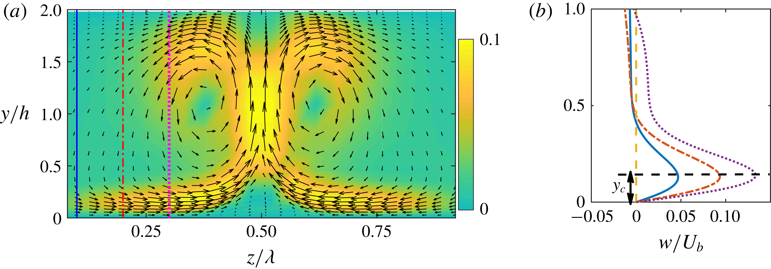
(a) Vector pattern of induced flow
 $(v,w)$
in the cross-stream (
 $y{-}z$
) plane with the colour denoting the velocity magnitude; (b) spanwise velocity profile (normalized with the bulk velocity) of the induced wall jet at different spanwise locations: the profiles are taken along the vertical lines shown in (a) at
 $z/\unicode[STIX]{x1D706}=0.1,0.2$
and
 $0.3$
.

Figure 1(a) shows the velocity field induced by the SOJF excitation with
 $A=0.005$
,
 $\unicode[STIX]{x1D6FD}=1$
and
 $\unicode[STIX]{x1D702}=18$
in the cross-stream (
 $y{-}z$
) plane. Note that the colliding wall jets turn upward and then backward constrained by the upper channel wall and then down back (downwash) toward the originating wall – thus forming the large-scale streamwise control swirls while also squashing the incoming wall jets. These swirls produce near their collision plane a pair of near-wall counter-rotating smaller (secondary) swirls of opposite sense to the primary swirls, which also affect the drag reduction performance. In particular, the tiny secondary swirls prevent the near-wall streaks on either side of the collision plane from merging, actually even strengthening and separating these two adjacent streaks; the resulting instability of these two strong streaks actually plays a role in creating streamwise vortices above the streak envelope. Figure 1(b) shows the corresponding spanwise velocity profiles at different spanwise locations; the maximum spanwise velocity is located at
 $y_{c}$
, which we use as the height of the wall jet. The profiles near the wall appear qualitatively similar to those generated by plasma actuators (inferred from the control flow vector patterns in Li et al. (Reference Li, Wong, Li, Zhang and Zhou2014); also, Thomas et al. (Reference Thomas, Corke, Hussain, Duong, McGowan, Jasinski and Simmons2016)).
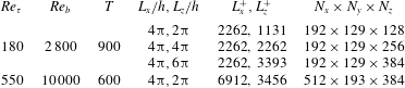
Details of the numerical discretization employed for the present simulations.

The current simulations of turbulent channel flows are based on the open-source finite difference software ‘Incompact3d’ (Laizet & Lamballais Reference Laizet and Lamballais2009; Laizet & Li Reference Laizet and Li2011), where periodicity in the streamwise and spanwise directions is imposed, and no-slip and impermeability conditions are applied at the walls. For the spatial derivatives, sixth-order compact schemes are used on a Cartesian grid stretched in the wall-normal direction. The time integration is performed using a low-storage third-order Runge–Kutta scheme. The pressure Poisson equation at each fractional step is solved using pseudo-spectral approach with appropriate three-dimensional fast Fourier transforms. Adopting the concept of modified wavenumbers, the divergence-free condition is ensured up to machine accuracy. In addition, the body force involved in our forcing method is also implemented in every sub-timestep. See Laizet & Lamballais (Reference Laizet and Lamballais2009), Laizet & Li (Reference Laizet and Li2011) for more details of the code and its validation, especially the treatment of the body force and pressure in spectral space. In the simulations, a constant flow rate is set and the bulk velocity
 $U_{b}$
(flow rate divided by the channel cross-section area) is maintained at a constant value. All computations start with the same initial condition of a fully developed turbulent channel flow without control (the mean, root-mean-square velocity and Reynolds shear stress profiles were checked against the standard database to ensure the initial flow state). Table 1 shows the numerical details used for different cases in the present study. About
 $90$
simulations were run with a control height
 $y_{c}^{+}=30$
at the friction Reynolds number around
 $Re_{\unicode[STIX]{x1D70F}}(\equiv u_{\unicode[STIX]{x1D70F}}h/\unicode[STIX]{x1D708})=180$
, corresponding to the bulk Reynolds number
 $Re_{b}(\equiv u_{b}h/\unicode[STIX]{x1D708})=2800$
. The computation domain is set to
 $4\unicode[STIX]{x03C0}\times 2\times 2\unicode[STIX]{x03C0}/4\unicode[STIX]{x03C0}/6\unicode[STIX]{x03C0}$
and discretized on a Cartesian grid of
 $n_{x}\times n_{y}\times n_{z}=192\times 129\times 128/256/384$
. Here, different spanwise sizes of the box are used to accommodate different forcing spacings. In addition, a few cases also explore how the drag reduction is sensitive to changes in
 $y_{c}^{+}$
, which varied in the range 5–100. To examine the control method at moderate
 $Re_{\unicode[STIX]{x1D70F}}$
, 45 simulations were also performed for different combinations of control parameters at
 $Re_{\unicode[STIX]{x1D70F}}=550$
, corresponding to
 $Re_{b}=10\,000$
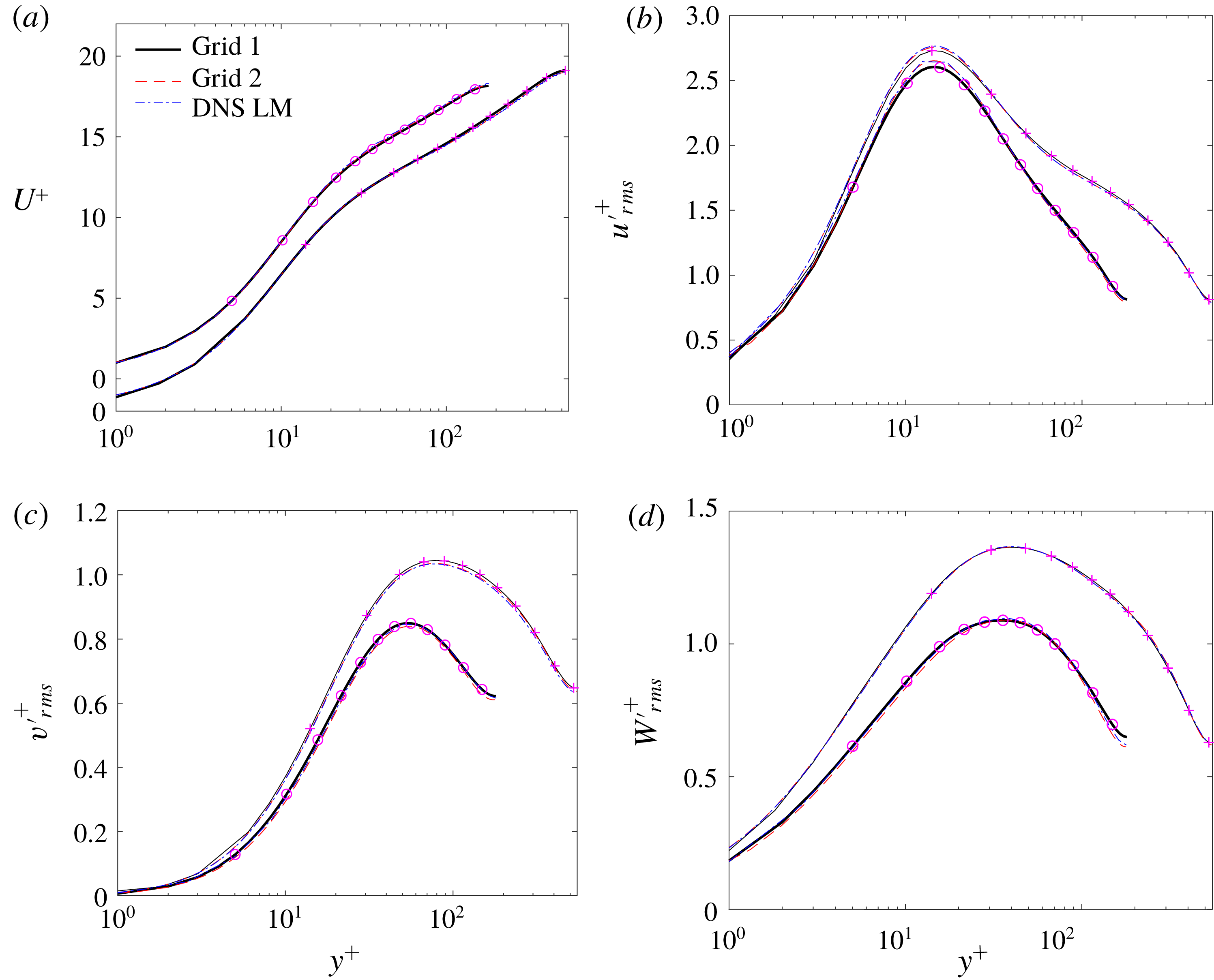
. The validation of the code, including the effects of the computational domain size and grid resolution, is provided in the Appendix.
We investigate how the forcing (2.3) changes the skin friction coefficient
 $C_{f}$
, defined as
 $$\begin{eqnarray}\displaystyle C_{f}=\frac{2\unicode[STIX]{x1D70F}_{w}}{\unicode[STIX]{x1D70C}U_{b}^{2}}, & & \displaystyle\end{eqnarray}$$
where
 $\unicode[STIX]{x1D70F}_{w}$
is the wall shear stress. The drag reduction
 ${\mathcal{R}}$
is quantified as the relative change in
 $C_{f}$
:
 $$\begin{eqnarray}\displaystyle {\mathcal{R}}=1-C_{f}/C_{f,0}, & & \displaystyle\end{eqnarray}$$
where
 $C_{f,0}$
is the skin friction coefficient of the reference (uncontrolled) flow. Note that,
 $C_{f}$
is evaluated by averaging over the entire channel wall area as well as over time after the initial transient when the flow adapts to the forcing and reaches the steady state; the averaging time (see table 1) is
 $900h/U_{b}$
and
 $600h/U_{b}$
for
 $Re_{\unicode[STIX]{x1D70F}}=180$
and
 $550$
, respectively. The transient time is estimated by direct observation of the time (
 $T$
) history of the space-averaged skin friction, which is typically of the order of
 $100\sim 300h/U_{b}$
as shown in Yao et al. (Reference Yao, Chen, Thomas and Hussain2017). For the drag reduction rate
 ${\mathcal{R}}$
, its uncertainty
 $\unicode[STIX]{x1D6FF}{\mathcal{R}}$
is calculated by following the procedure in Gatti & Quadrio (Reference Gatti and Quadrio2016), summarized as follows. First, the standard uncertainty
 $\unicode[STIX]{x1D70E}_{C_{f}}$
of
 $C_{f}$
is calculated via an autoregressive method as described by Oliver et al. (Reference Oliver, Malaya, Ulerich and Moser2014). Then the standard uncertainty
 $\unicode[STIX]{x1D70E}_{{\mathcal{R}}}$
of
 ${\mathcal{R}}$
is obtained by propagating the standard uncertainty of
 $C_{f}$
for the uncontrolled and controlled cases (assuming they are independent variables (Gatti & Quadrio Reference Gatti and Quadrio2013)), i.e.
 $\unicode[STIX]{x1D70E}_{{\mathcal{R}}}=(C_{f}/C_{f,0})\sqrt{(\unicode[STIX]{x1D70E}_{C_{f}}/C_{f})^{2}+(\unicode[STIX]{x1D70E}_{C_{f,0}}/C_{f,0})^{2}}$
. Finally, the uncertainty is extended to a
 $95\,\%$
confidence interval
 $\unicode[STIX]{x1D6FF}{\mathcal{R}}=z\unicode[STIX]{x1D70E}_{{\mathcal{R}}}$
, here
 $z=1.96$
is the standardized
 $95\,\%$
confidence interval of a normalized Gaussian probability density function. The uncertainty of
 ${\mathcal{R}}$
is reported in the text when applicable and plotted as error bar in the relevant figures.
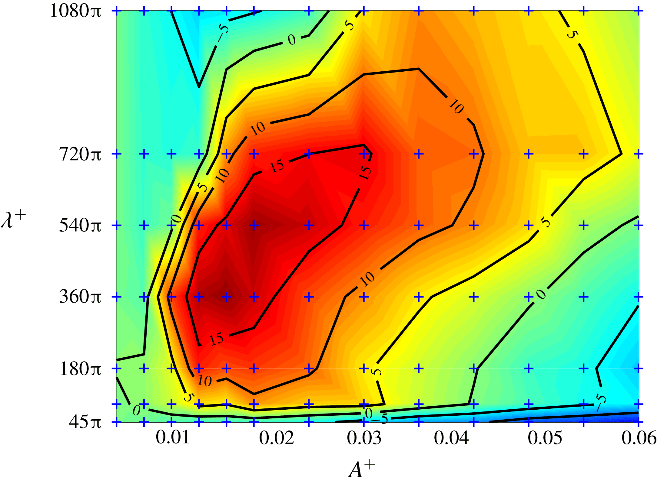
Drag reduction rate
 ${\mathcal{R}}$
(
 $\%$
) as a function of
 $A^{+}$
and
 $\unicode[STIX]{x1D706}^{+}$
for
 $y_{c}^{+}=30$
at
 $Re_{\unicode[STIX]{x1D70F}}=180$
. In this figure, the symbol
 $+$
indicates the simulation data points used for interpolation.

3 Parametric study for
 $Re_{\unicode[STIX]{x1D70F}}=180$

Consideration is first given to the effects of different forcing spacings and amplitudes. Figure 2 shows the drag reduction
 ${\mathcal{R}}$
as a function of
 $A^{+}$
and
 $\unicode[STIX]{x1D706}^{+}$
for
 $y_{c}^{+}=30$
(this choice of
 $y_{c}^{+}$
is discussed later) at
 $Re_{\unicode[STIX]{x1D70F}}=180$
. The computations with forcing are carried out at seven different spacings
 $\unicode[STIX]{x1D706}^{+}$
ranging from
 $45\unicode[STIX]{x03C0}$
to
 $1080\unicode[STIX]{x03C0}$
, corresponding to a simultaneous control of
 $1$
to
 $35$
low-speed streaks (noting that the mean spanwise spacing of the streaks
 $\unicode[STIX]{x1D706}_{z}^{+}\approx 100$
in the near-wall region (Kline et al.
Reference Kline, Reynolds, Schraub and Runstadler1967; Smith & Metzler Reference Smith and Metzler1983)). Also,
 $13$
different amplitudes in the range
 $0.003\leqslant A^{+}\leqslant 0.06$
are chosen. Thus,
 $91$
total simulations are performed covering various
 $A^{+}$
and
 $\unicode[STIX]{x1D706}^{+}$
values. The contours are computed from a linear interpolation of these discrete simulated points. It is rather impressive that
 ${\mathcal{R}}$
can be obtained in broad ranges of forcing amplitude and wavelength – a decidedly robust feature as precise selection and adherence to a particular value is not critical.
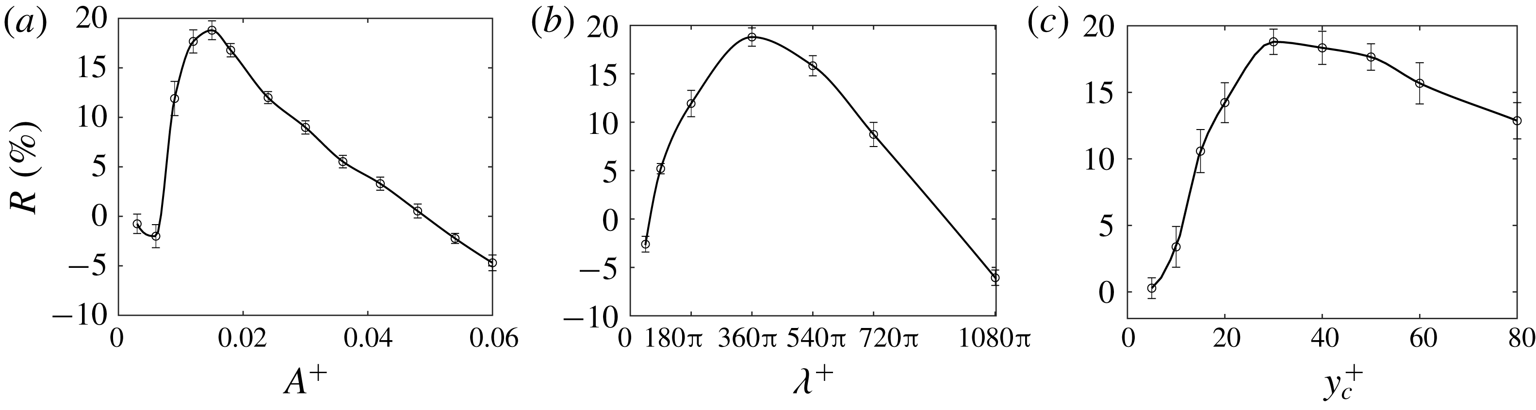
Drag reduction rate
 ${\mathcal{R}}$
(a) as a function of
 $A^{+}$
for
 $\unicode[STIX]{x1D706}^{+}=360$
at
 $y_{c}^{+}=30$
; (b) as a function of
 $\unicode[STIX]{x1D706}^{+}$
for
 $A^{+}=0.015$
at
 $y_{c}^{+}=30$
; (c) as a function of
 $y_{c}^{+}$
for
 $A^{+}=0.015$
and
 $\unicode[STIX]{x1D706}^{+}=360\unicode[STIX]{x03C0}$
. The error bar indicates the corresponding uncertainty of
 ${\mathcal{R}}$
.

Figure 3(a) shows a non-monotonic variation of drag reduction
 ${\mathcal{R}}$
as a function of
 $A^{+}$
at
 $\unicode[STIX]{x1D706}^{+}=360\unicode[STIX]{x03C0}$
and
 $y_{c}^{+}=30$
. At small amplitudes, i.e.
 $A^{+}<0.006$
, there is a slight drag increase, because the control flow is too weak to push streaks to merge, while additional Reynolds shear stresses are generated by the forcing, hence causing drag increase. As
 $A^{+}$
increases, suppression of Reynolds shear stress overcomes its enhancement due to merging of streaks, hence leading to drag reduction. The optimal
 ${\mathcal{R}}$
is
 $18.6\,\%\pm 0.9\,\%$
at
 $A^{+}=0.015$
, and
 ${\mathcal{R}}$
deteriorates with increasing
 $A^{+}$
. At
 $A^{+}=0.06$
(the largest forcing amplitude considered in this paper),
 ${\mathcal{R}}$
is actually increased by
 $4.1\,\%\pm 0.5\,\%$
.
Similar trend is also found for
 $\unicode[STIX]{x1D706}^{+}$
. If
 $\unicode[STIX]{x1D706}^{+}$
is too small (less than the spacing of two streaks), the control flow leads to no streak merging and hence no drag reduction. On the other hand, at much larger
 $\unicode[STIX]{x1D706}^{+}$
, the forcing is spread over in a larger spanwise domain, which is ineffective at causing the streaks to merge. Figure 3(b) shows
 ${\mathcal{R}}$
as a function of forcing spacing
 $\unicode[STIX]{x1D706}^{+}$
at
 $A^{+}=0.015$
and
 $y_{c}^{+}=30$
. Clearly,
 ${\mathcal{R}}$
increases with increasing
 $\unicode[STIX]{x1D706}^{+}$
for
 $\unicode[STIX]{x1D706}^{+}\leqslant 360\unicode[STIX]{x03C0}$
, but becomes less effective for
 $\unicode[STIX]{x1D706}^{+}>360\unicode[STIX]{x03C0}$
. The maximum
 ${\mathcal{R}}$
is approximately
 $18.6\,\%\pm 0.9\,\%$
and occurs at
 $\unicode[STIX]{x1D706}^{+}=360\unicode[STIX]{x03C0}$
, corresponding to a simultaneous control of approximately
 $10-15$
streaks by each swirl pair. Note the small drag increase (by
 $2.5\,\%\pm 0.8\,\%$
) at
 $\unicode[STIX]{x1D706}^{+}=45\unicode[STIX]{x03C0}$
, where there is no merger of streaks (since the control spacing
 $\unicode[STIX]{x1D706}^{+}\approx 140$
is close to the streak spacing) whilst the additional drag is caused by the Reynolds shear stress generated by the controlling swirls. Another feature of figure 3(b) is that there is a wide range of forcing spacing (i.e.
 $60\unicode[STIX]{x03C0}\lesssim \unicode[STIX]{x1D706}^{+}\lesssim 900\unicode[STIX]{x03C0}$
) over which
 ${\mathcal{R}}$
is achieved.
Note that the optimal spacing
 $\unicode[STIX]{x1D706}^{+}=360\unicode[STIX]{x03C0}$
in this paper is consistent with the optimal wavelength
 $\unicode[STIX]{x1D706}^{+}=1200$
found by Canton et al. (Reference Canton, Örlü, Chin, Hutchins, Monty and Schlatter2016a
). Interestingly,
 $\unicode[STIX]{x1D706}^{+}=360\unicode[STIX]{x03C0}$
also matches well with the optimal value of several other drag reduction techniques. For example, similar spanwise modulation scales are also found by Berger et al. (Reference Berger, Kim, Lee and Lim2000) in their Lorentz forcing control, Ricco & Hahn (Reference Ricco and Hahn2013) in their rotating disk wall control, Ghebali, Chernyshenko & Leschziner (Reference Ghebali, Chernyshenko and Leschziner2017) in their wavy wall configurations. However, the optimal spanwise spacing in some other strategies is quite different; for example, Segawa et al. (Reference Segawa, Mizunuma, Murakami, Li and Yoshida2007) obtain a maximum
 ${\mathcal{R}}$
of 5–7 % utilizing the alternating blowing and suction configurations whose spanwise spacing is only 300 (
 $+$
units). As for spanwise wall oscillation control, a characteristic spanwise displacement 1400 (
 $+$
unit) can be obtained based on the study of Jung et al. (Reference Jung, Mangiavacchi and Akhavan1992) by converting their optimal oscillating period to the spanwise spacing. However, since the drag reduction increases with the maximum wall velocity (Quadrio & Ricco Reference Quadrio and Ricco2004; Yakeno et al.
Reference Yakeno, Hasegawa and Kasagi2014), there seems to be no optimal spanwise wall displacement for the spanwise wall oscillation method. It would be interesting to compare these seemingly different control methods and to determine the underline physical mechanism for the selection of the optimal wavelength or oscillation period.
The effect of different control heights
 $y_{c}^{+}$
on drag reduction
 ${\mathcal{R}}$
is considered here. Note that a complete investigation of the effect of
 $y_{c}^{+}$
under the variation of other two controlling parameters is a computational challenge. Hence, for illustration, only the optimal spacing (
 $\unicode[STIX]{x1D706}^{+}=360\unicode[STIX]{x03C0}$
) and amplitude (
 $A^{+}=0.015$
) identified above are considered here. In fact, we also find similar amounts of
 ${\mathcal{R}}$
when
 $\unicode[STIX]{x1D706}^{+}$
and
 $A^{+}$
both increase, e.g.
 ${\mathcal{R}}=18.3\,\%\pm 0.9\,\%$
can be achieved at
 $\unicode[STIX]{x1D706}^{+}=540\unicode[STIX]{x03C0}$
and
 $A^{+}=0.018$
. However, the smaller
 $A^{+}$
is obviously preferred as less energy input is required (discussed in § 5.1). Figure 3(c) shows
 ${\mathcal{R}}$
for different
 $y_{c}^{+}$
at
 $A^{+}=0.015$
and
 $\unicode[STIX]{x1D706}^{+}=360\unicode[STIX]{x03C0}$
, where the optimal
 $y_{c}^{+}$
is
 $30$
. For a smaller
 $y_{c}^{+}$
(say,
 $=5$
),
 ${\mathcal{R}}$
is only
 $1.4\,\%\pm 0.7\,\%$
, because the wall jet is too thin to affect most parts of the streaks. For a much larger
 $y_{c}^{+}$
(say,
 $=80$
),
 ${\mathcal{R}}$
is
 $13.5\pm 1.1\,\%$
. Note that as
 $y_{c}^{+}$
increases, the downwash of the primary swirls, due to the constraint of the upper wall, becomes strong enough to increase drag, and the secondary swirls are also larger and stronger, so that their own high momentum downwash will increase the skin friction. These two effects combine together to decrease the effect of
 ${\mathcal{R}}$
imposed by the control flow and may even cause drag increase as
 $y_{c}^{+}$
increases. Thus, we conclude that a too large
 $y_{c}^{+}$
is to be avoided at high
 $Re$
.
4 Analysis of drag reduction
To understand the mechanisms of both drag reduction and increase by the forcing, flow statistics as well as the dynamics are examined in detail below for the effects of
 $A^{+}$
and
 $y_{c}^{+}$
only. We focus only on these two parameters as we consider them to be the more important of the three, in order to limit the scope and size of the paper.
4.1 Triple decomposition
In view of the steady control flow, different from both the mean flow and turbulent fluctuations, it seems natural to interpret the total flow from the perspective of the following three components by using the triple decomposition (Reynolds & Hussain Reference Reynolds and Hussain1972):
 $$\begin{eqnarray}\displaystyle \boldsymbol{u}(x,y,z,t)=\boldsymbol{U}(y)+\underbrace{\tilde{\boldsymbol{u}}(y,z)+\boldsymbol{u}^{\prime \prime }(x,y,z,t)}_{\boldsymbol{u}^{\prime }}. & & \displaystyle\end{eqnarray}$$
Here,
 $\boldsymbol{u}$
is the instantaneous total velocity field;
 $\boldsymbol{U}=\langle \overline{\boldsymbol{u}}\rangle$
is the mean velocity, where the overbar indicates averaging in time and in the streamwise direction – and also includes averaging in the spanwise direction if more than one spanwise wavelength is contained in the computational domain; and the bracket
 $\langle \boldsymbol{\cdot }\rangle$
indicates spanwise averaging over one period;
 $\boldsymbol{u}^{\prime }=\boldsymbol{u}-\boldsymbol{U}$
is the total fluctuation;
 $\tilde{\boldsymbol{u}}=\overline{\boldsymbol{u}}-\boldsymbol{U}$
is the so-called ‘organized field’ representing the coherent motion induced by the swirls; and
 $\boldsymbol{u}^{\prime \prime }=\boldsymbol{u}-\overline{\boldsymbol{u}}$
is the random turbulent fluctuation.
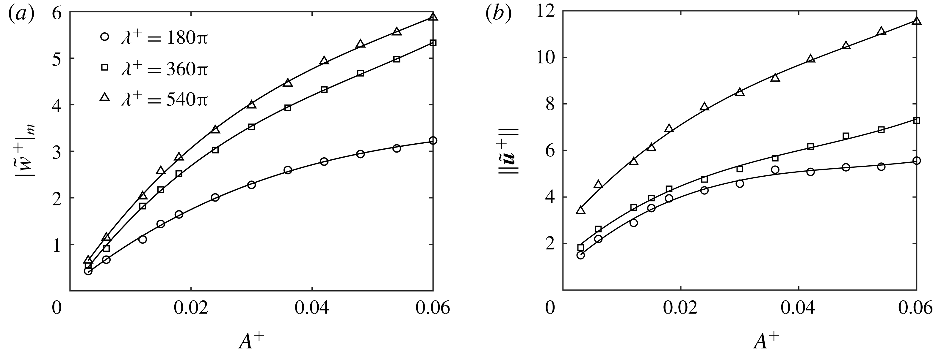
Forcing amplitude (
 $A^{+}$
) dependence: (a) the maximum mean spanwise velocity
 $|\tilde{w}|_{m}$
and (b)
 $\Vert \tilde{\boldsymbol{u}}\Vert$
at
 $Re_{\unicode[STIX]{x1D70F}}=180$
. Superscript
 $+$
indicates scaling with
 $u_{\unicode[STIX]{x1D70F}}$
of uncontrolled flow. Different symbols represent different controlling wavenumbers
 $\unicode[STIX]{x1D706}^{+}$
.

Since the forcing amplitude
 $A^{+}$
does not correspond to a directly measurable quantity in the flow, two quantities, based on
 $\tilde{\boldsymbol{u}}$
, are employed to characterize the flow response to the forcing. The first one is the maximum mean spanwise velocity
 $|\tilde{w}|_{m}=\max \{|\tilde{w}|\}$
, which characterizes the strength of the spanwise wall-jet motion. The second one is chosen to be the norm of
 $\tilde{\boldsymbol{u}}$
,
 $$\begin{eqnarray}\displaystyle \Vert \tilde{\boldsymbol{u}}\Vert =\sqrt{\frac{1}{\unicode[STIX]{x1D6FA}}\int _{\unicode[STIX]{x1D6FA}}\tilde{\boldsymbol{u}}\boldsymbol{\cdot }\tilde{\boldsymbol{u}}\,\text{d}\unicode[STIX]{x1D6FA}}, & & \displaystyle\end{eqnarray}$$
where
 $\unicode[STIX]{x1D6FA}$
is the total volume of the computational domain.
 $\Vert \tilde{\boldsymbol{u}}\Vert$
represents the volume-averaged kinetic energy of the induced motion. The variations of the two quantities as a function of the forcing amplitude are shown in figure 4 for three different
 $\unicode[STIX]{x1D706}^{+}$
values. As expected, both
 $|\tilde{w}|_{m}$
and
 $\Vert \tilde{\boldsymbol{u}}\Vert$
increase with increasing
 $A^{+}$
and
 $\unicode[STIX]{x1D706}^{+}$
. In addition, we also find that, at a given
 $A^{+}$
, the increase of
 $|\tilde{w}|_{m}$
with the increase of
 $\unicode[STIX]{x1D706}^{+}$
becomes slower, in comparison to the faster increase of
 $\Vert \tilde{\boldsymbol{u}}\Vert$
with
 $\unicode[STIX]{x1D706}^{+}$
, which implies the ineffectiveness of a large forcing spacing, since more energy input is required to generate similar strengths of the spanwise wall-jet velocity as with small spacing. Interestingly, for high
 ${\mathcal{R}}$
cases,
 $|\tilde{w}|_{m}\approx 2\sim 4u_{\unicode[STIX]{x1D70F},0}$
, which is very close to the optimal spanwise perturbation velocity introduced by plasma actuators in TBL control (Thomas et al.
Reference Thomas, Corke, Hussain, Duong, McGowan, Jasinski and Simmons2016).
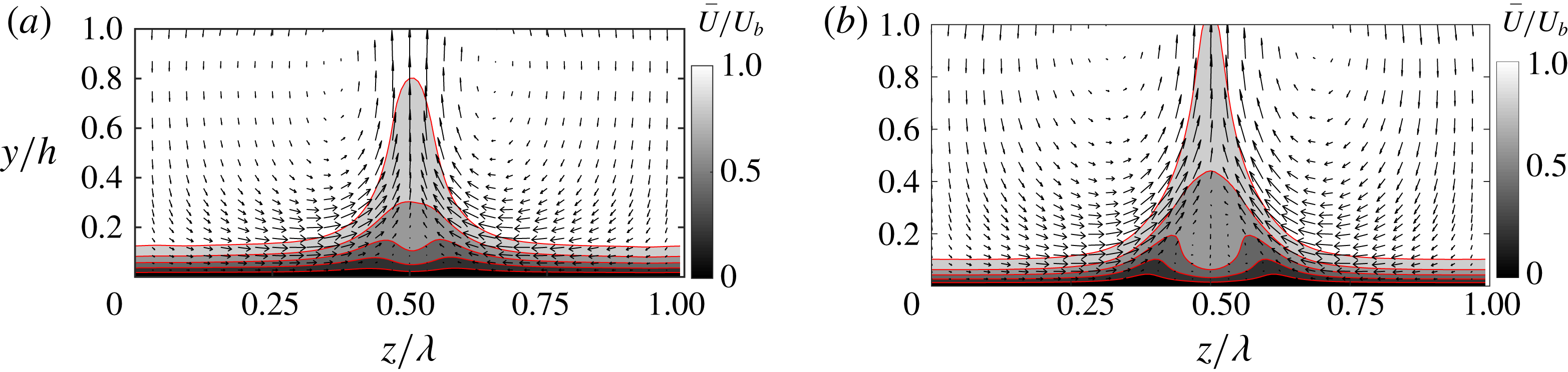
Cross-stream (
 $y{-}z$
) plane view of mean velocity field (
 $\overline{\boldsymbol{u}}$
) with the contours indicating the mean streamwise velocity (normalized by the bulk velocity
 $U_{b}$
), and the vectors denoting the wall-normal and spanwise velocities for (a)
 $A^{+}=0.015$
; (b)
 $A^{+}=0.06$
with
 $\unicode[STIX]{x1D706}^{+}=360\unicode[STIX]{x03C0}$
and
 $y_{c}^{+}=30$
.

Figure 5(a,b) shows the cross-streamwise view (
 $y{-}z$
plane) of contours of the streamwise velocity and the cross-plane velocity vectors of
 $\overline{\boldsymbol{u}}$
at two different forcing amplitudes
 $A^{+}=0.015$
(corresponding to the optimal control case) and
 $A^{+}=0.06$
(corresponding to a drag increase case) with
 $\unicode[STIX]{x1D706}^{+}=360\unicode[STIX]{x03C0}$
and
 $y_{c}^{+}=30$
. For
 $A^{+}=0.015$
, the topmost low-speed streak envelope, which has only one peak, is due to the lift-up effect of the counter-rotating control swirls, and extends up to the outer flow region (
 $y/h>0.6$
). Near the wall, however, the streak has dual peaks, which are due to the secondary swirls. As the forcing amplitude increases to
 $A^{+}=0.06$
, the lift-up effect of the control swirls becomes even stronger; and the topmost low-speed streak extends up to the half-channel height. In addition, the near-wall streaks fall apart more due to the effect of stronger secondary swirls.
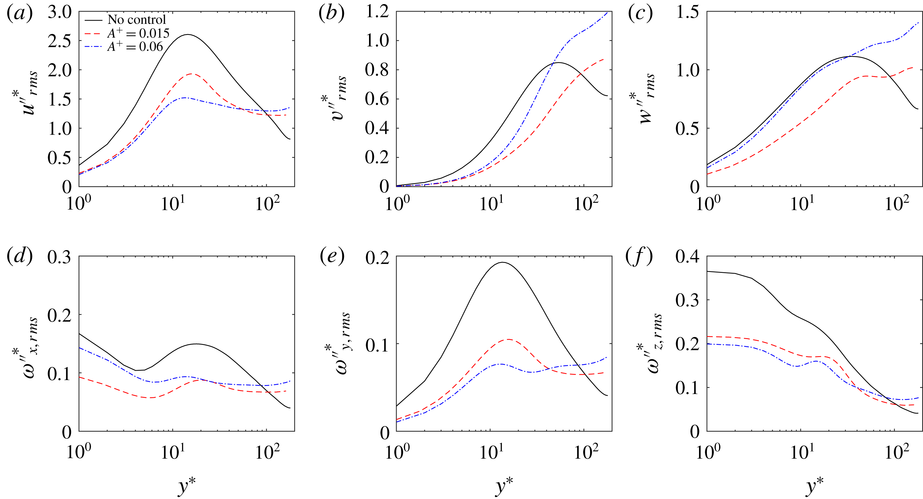
To compare the turbulent fluctuations with those in the uncontrolled case, figure 6 shows the spanwise-averaged velocity
 $\{\langle \overline{u_{i}^{\prime \prime 2}}\rangle ^{1/2}\}^{\ast }$
and vorticity
 $\{\langle \overline{\unicode[STIX]{x1D714}_{i}^{\prime \prime 2}}\rangle ^{1/2}\}^{\ast }$
fluctuations at two forcing magnitudes
 $A^{+}=0.015$
and
 $0.06$
(the superscript
 $\ast$
indicates non-dimensionalization by the wall units of the controlled flow). All of the velocity and vorticity fluctuations are suppressed near the wall due to the merger of numerous streaks and hence fewer streamwise vortices are regenerated under control; however, they are all enhanced in the outer region (
 $y/h>0.6$
), mainly due to the advection of the large-scale control swirls, which transport the near-wall turbulence and vortical structures to the outer flow (see § 4.3). Notable differences are also observed by comparing
 $A^{+}=0.015$
and
 $0.06$
. In the outer region, all the turbulent fluctuations are further increased for the
 $A^{+}=0.06$
case, which is, as expected, due to the even stronger advection effect of the control swirls. In the near wall, the root mean square (r.m.s.) of
 $v^{\prime \prime }$
,
 $w^{\prime \prime }$
and
 $\unicode[STIX]{x1D714}_{x}^{\prime \prime }$
are increased, and
 $u^{\prime \prime }$
,
 $\unicode[STIX]{x1D714}_{y}^{\prime \prime }$
and
 $\unicode[STIX]{x1D714}_{z}^{\prime \prime }$
are decreased, which is consistent with figure 13(e) where more streamwise aligned vortices are observed near the collision region of two swirls.
Spanwise-averaged turbulent velocity (top row) and vorticity (bottom row) fluctuations with various forcing amplitudes for
 $\unicode[STIX]{x1D706}^{+}=360\unicode[STIX]{x03C0}$
and
 $y_{c}^{+}=30$
. Solid line: uncontrolled case; dashed line: drag reduction with
 $A^{+}=0.015$
; dash-dotted line: drag increase with
 $A^{+}=0.06$
.

4.2 Scales of drag production
To analyse the contribution of the drag coefficient, the FIK (Fukagata, Iwamoto, Kasagi) identity (Fukagata et al.
Reference Fukagata, Iwamoto and Kasagi2002; Rastegari & Akhavan Reference Rastegari and Akhavan2015), which links the skin friction with the total Reynolds shear stress
 $\langle \overline{u^{\prime }v^{\prime }}\rangle$
, is invoked:
 $$\begin{eqnarray}\displaystyle C_{f}=\underbrace{\frac{12}{Re_{b}}}_{C_{f}^{L}}+\underbrace{12\int _{0}^{2}(1-y)\left(-\frac{\langle \overline{u^{\prime }v^{\prime }}\rangle }{4U_{b}^{2}}\right)\,\text{d}y}_{C_{f}^{T}}. & & \displaystyle\end{eqnarray}$$
The drag coefficient
 $C_{f}$
thus has an ‘equivalent’ laminar part
 $C_{f}^{L}=12/Re_{b}$
, and a turbulent part
 $C_{f}^{T}$
represented by the weighted integration of the total Reynolds shear stress (RSS)
 $\langle \overline{u^{\prime }v^{\prime }}\rangle$
. As the latter is composed of a coherent part
 $\langle \tilde{u} \tilde{v}\rangle$
and a random part
 $\langle \overline{u^{\prime \prime }v^{\prime \prime }}\rangle$
, the FIK identity can be further decomposed as
 $$\begin{eqnarray}\displaystyle C_{f}=\underbrace{\frac{12}{Re_{b}}}_{C_{f}^{L}}+\underbrace{12\int _{0}^{2}(1-y)\left(-\frac{\langle \tilde{u} \tilde{v}\rangle }{4U_{b}^{2}}\right)\,\text{d}y}_{C_{f}^{C}}+\underbrace{12\int _{0}^{2}(1-y)\left(-\frac{\langle \overline{u^{\prime \prime }v^{\prime \prime }}\rangle }{4U_{b}^{2}}\right)\,\text{d}y}_{C_{f}^{R}}. & & \displaystyle\end{eqnarray}$$
Since
 $Re_{b}$
is held constant in all simulations under different control parameters, only changes in the other two parts (coherent
 $C_{f}^{C}$
and random
 $C_{f}^{R}$
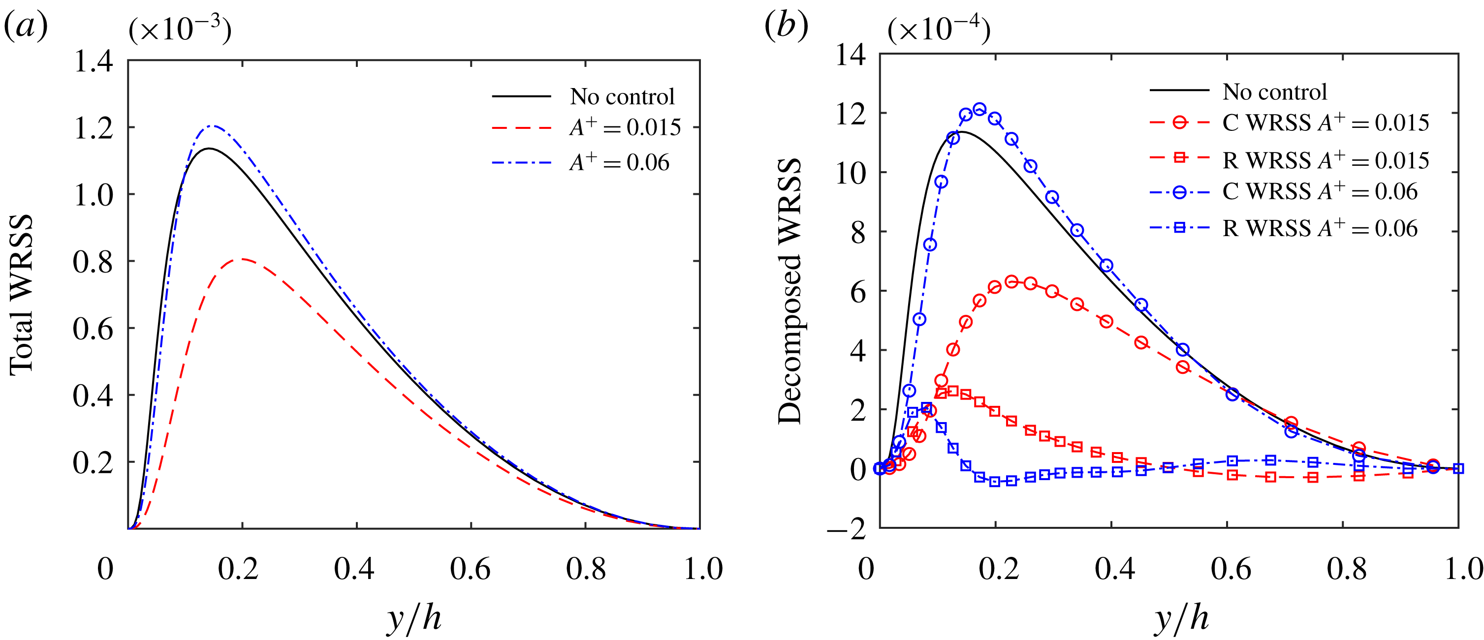
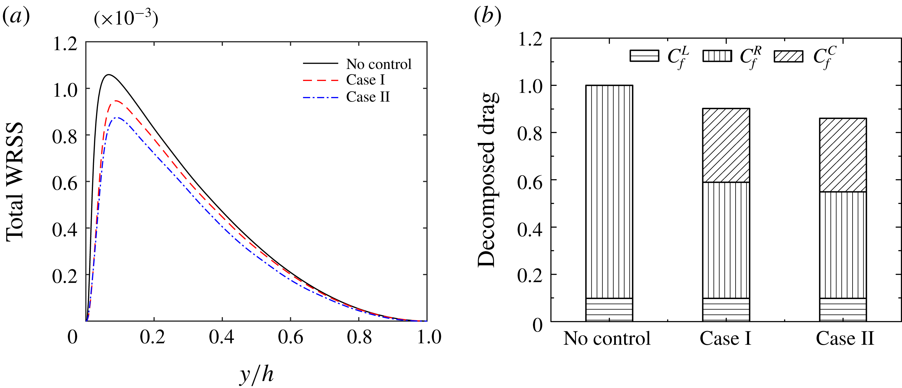
) affect the drag. Figure 7(a) shows the profiles of the total weighted Reynolds shear stress (WRSS)
 $-(1-y)\langle \overline{u^{\prime }v^{\prime }}\rangle$
, and figure 7(b) shows the coherent part
 $-(1-y)\langle \tilde{u} \tilde{v}\rangle$
(denoted as C-WRSS) and the random part
 $-(1-y)\langle \overline{u^{\prime \prime }v^{\prime \prime }}\rangle$
(denoted as R-WRSS). For the low amplitude
 $A^{+}=0.015$
case, the drag reduction, following (4.3), is due to the alteration of the Reynolds shear stress throughout the whole range of
 $y$
. Further, from figure 7(b), we find that the random turbulent Reynolds shear stress is significantly suppressed, and the coherent part contributes the most to the total Reynolds shear stress. In contrast, at a very high amplitude (
 $A^{+}=0.06$
), the drag increment is due to the enhancement of the coherent Reynolds shear stress away from the wall (
 $y^{+}>20$
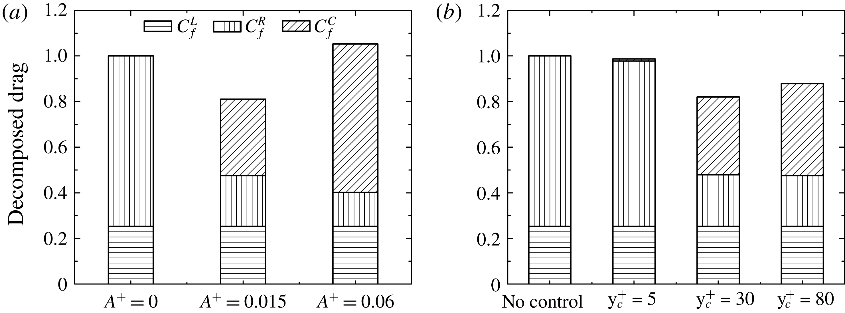
). This also can be clearly shown through the decomposed total skin friction (normalized by the uncontrolled total skin friction) in figure 8(a). For the uncontrolled case (no coherent part), the laminar part contributes 25.0 % to the skin friction, and the turbulent part contributes 75.0 %. For
 $A^{+}=0.015$
, the random part contribution is reduced to 22.6 %, and the coherent part increased to 33.8 %; hence the net skin friction is reduced by 18.6 %. In contrast, for a higher
 $A^{+}=0.06$
, although the random turbulent part is reduced to approximately 15.5 %, the coherent part is increased to 63.6 %, hence leading to the net skin friction increase of 4.1 %. (Note that figure 8(b) shows a similar analysis of
 $C_{f}$
for the effect of different
 $y_{c}^{+}$
, to be discussed in § 4.4.) Therefore, effective drag reduction results from a compensative effect of suppressing random turbulence (via suppression of the streaks as well as the streamwise vortices) countered by enhancing the coherent part induced by the energetic forcing.
(a) Total and (b) decomposed weighted Reynolds shear stress (WRSS) distributions for different control amplitudes
 $A^{+}$
with
 $\unicode[STIX]{x1D706}^{+}=360\unicode[STIX]{x03C0}$
and
 $y_{c}^{+}=30$
at
 $Re_{\unicode[STIX]{x1D70F}}=180$
.

To quantify the contributions to the skin friction from different scales, the FIK identity in combination with the spanwise wavenumber spectrum of the Reynolds shear stress is also employed (see also de Giovanetti, Hwang & Choi (Reference de Giovanetti, Hwang and Choi2016)). (These contributions do not exist independently because different scales results from nonlinear interactions among them.) The total Reynolds shear stress can be expressed in terms of the one-dimensional spanwise Reynolds shear stress spectral density
 $\unicode[STIX]{x1D6F7}^{T}(y;k_{z})$
, i.e.
 $$\begin{eqnarray}\displaystyle -\langle \overline{u^{\prime }v^{\prime }}\rangle =\int _{-\infty }^{\infty }\unicode[STIX]{x1D6F7}^{T}(y;k_{z})\,\text{d}k_{z}, & & \displaystyle\end{eqnarray}$$
where
 $k_{z}(=2\unicode[STIX]{x03C0}/\unicode[STIX]{x1D706}_{z})$
is the spanwise wavenumber. Then, the Reynolds shear stress contributed by the motions with spanwise size
 $\unicode[STIX]{x1D706}_{z}$
smaller than a given cutoff wavelength
 $\unicode[STIX]{x1D706}_{z,c}$
is:
 $$\begin{eqnarray}\displaystyle -\langle \overline{u^{\prime }v^{\prime }}\rangle _{c}(y;\unicode[STIX]{x1D706}_{z,c})=2\int _{k_{z,c}}^{\infty }\unicode[STIX]{x1D6F7}^{T}(y;k_{z})\,\text{d}k_{z}, & & \displaystyle\end{eqnarray}$$
where the cutoff wavenumber is
 $k_{z,c}=2\unicode[STIX]{x03C0}/\unicode[STIX]{x1D706}_{z,c}$
. The above spanwise spectrum analysis can be similarly applied to the coherent Reynolds shear stress
 $-\langle \tilde{u} \tilde{v}\rangle _{c}=2\int _{k_{z,c}}^{\infty }\unicode[STIX]{x1D6F7}^{C}(y;k_{z})\,\text{d}k_{z}$
and the random turbulent stress
 $-\langle \overline{u^{\prime \prime }v^{\prime \prime }}\rangle _{c}=2\int _{k_{z,c}}^{\infty }\unicode[STIX]{x1D6F7}^{R}(y;k_{z})\,\text{d}k_{z}$
. Therefore, one obtains the skin friction coefficient generated by the motions with
 $\unicode[STIX]{x1D706}_{z}<\unicode[STIX]{x1D706}_{z,c}$
:
 $$\begin{eqnarray}\displaystyle C_{f,c}(\unicode[STIX]{x1D706}_{z,c}) & = & \displaystyle \frac{12}{Re_{b}}+\underbrace{12\int _{0}^{2}(1-y)\left(-\frac{\langle \overline{u^{\prime }v^{\prime }}\rangle _{c}}{4U_{b}^{2}}\right)\text{d}y}_{C_{f,c}^{T}}\nonumber\\ \displaystyle & = & \displaystyle \frac{12}{Re_{b}}+\underbrace{12\int _{0}^{2}(1-y)\left(-\frac{\langle \tilde{u} \tilde{v}\rangle _{c}}{4U_{b}^{2}}\right)\text{d}y}_{C_{f,c}^{C}}+\underbrace{12\int _{0}^{2}(1-y)\left(-\frac{\langle \overline{u^{\prime \prime }v^{\prime \prime }}\rangle _{c}}{4U_{b}^{2}}\right)\text{d}y}_{C_{f,c}^{R}},\nonumber\\ \displaystyle & & \displaystyle\end{eqnarray}$$
which provides a tool to estimate the amount of drag contributed by coherent motions and random turbulent fluctuations of different scales.
The decomposed drag (
 $C_{f}^{L}$
,
 $C_{f}^{C}$
,
 $C_{f}^{R}$
) for (a) different
 $A^{+}$
and (b) different
 $y_{c}^{+}$
at
 $Re_{\unicode[STIX]{x1D70F}}=180$
.

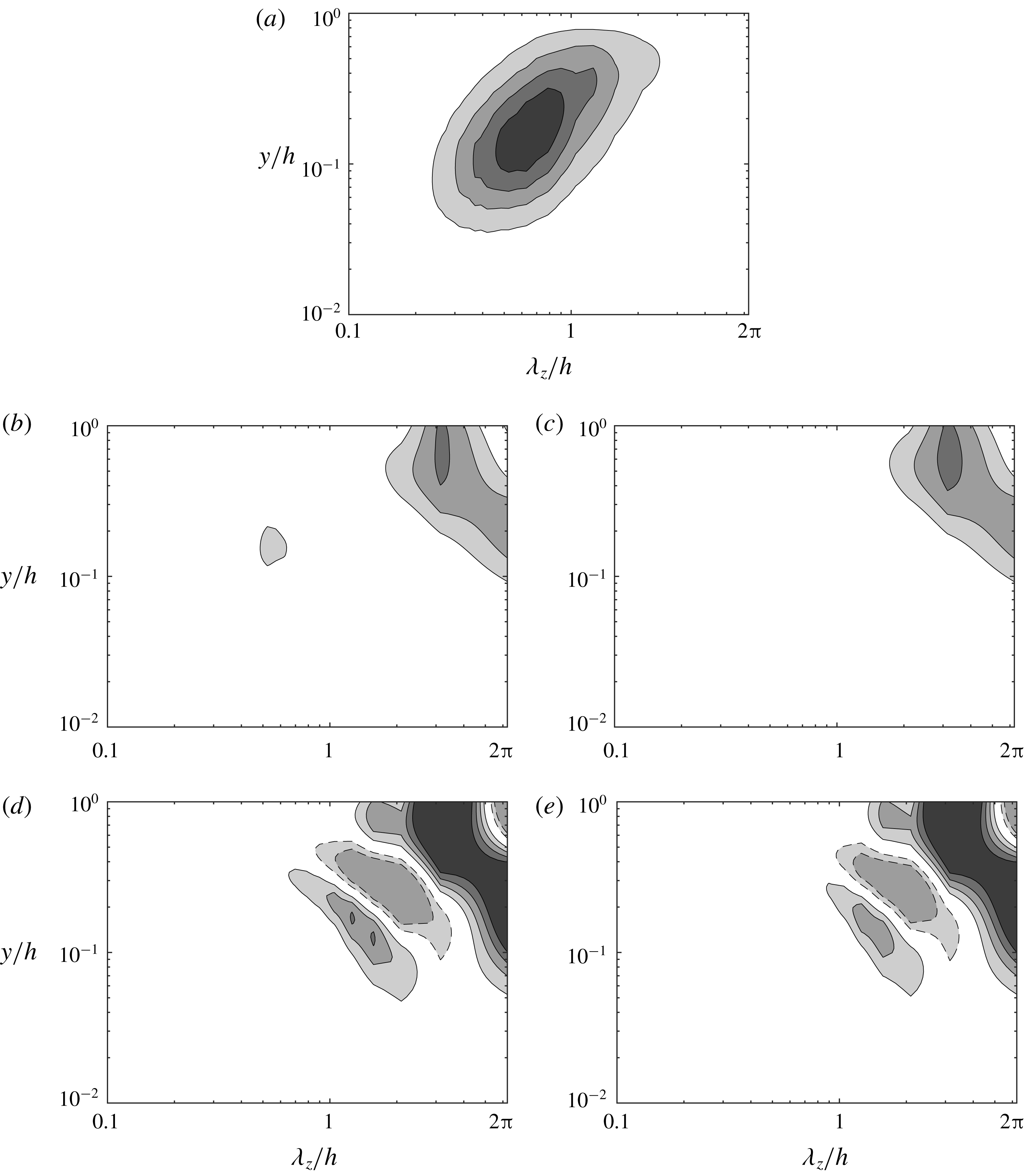
Premultiplied spanwise wavenumber spectra of the total Reynolds shear stress
 $k_{z}\unicode[STIX]{x1D6F7}_{uv}^{T}$
for (a) uncontrolled flow; (b)
 $A^{+}=0.015$
; and (d)
 $A^{+}=0.06$
, and the coherent Reynolds shear stress
 $k_{z}\unicode[STIX]{x1D6F7}_{uv}^{C}$
for (c)
 $A^{+}=0.015$
, and (e)
 $A^{+}=0.06$
. The contour labels indicate 0.2, 0.4, 0.6 and 0.8 of the maximum value of the uncontrolled case, and dashed lines for negative values.

The premultiplied spanwise wavenumber spectrum of the Reynolds shear stress
 $k_{z}\unicode[STIX]{x1D6F7}^{T}$
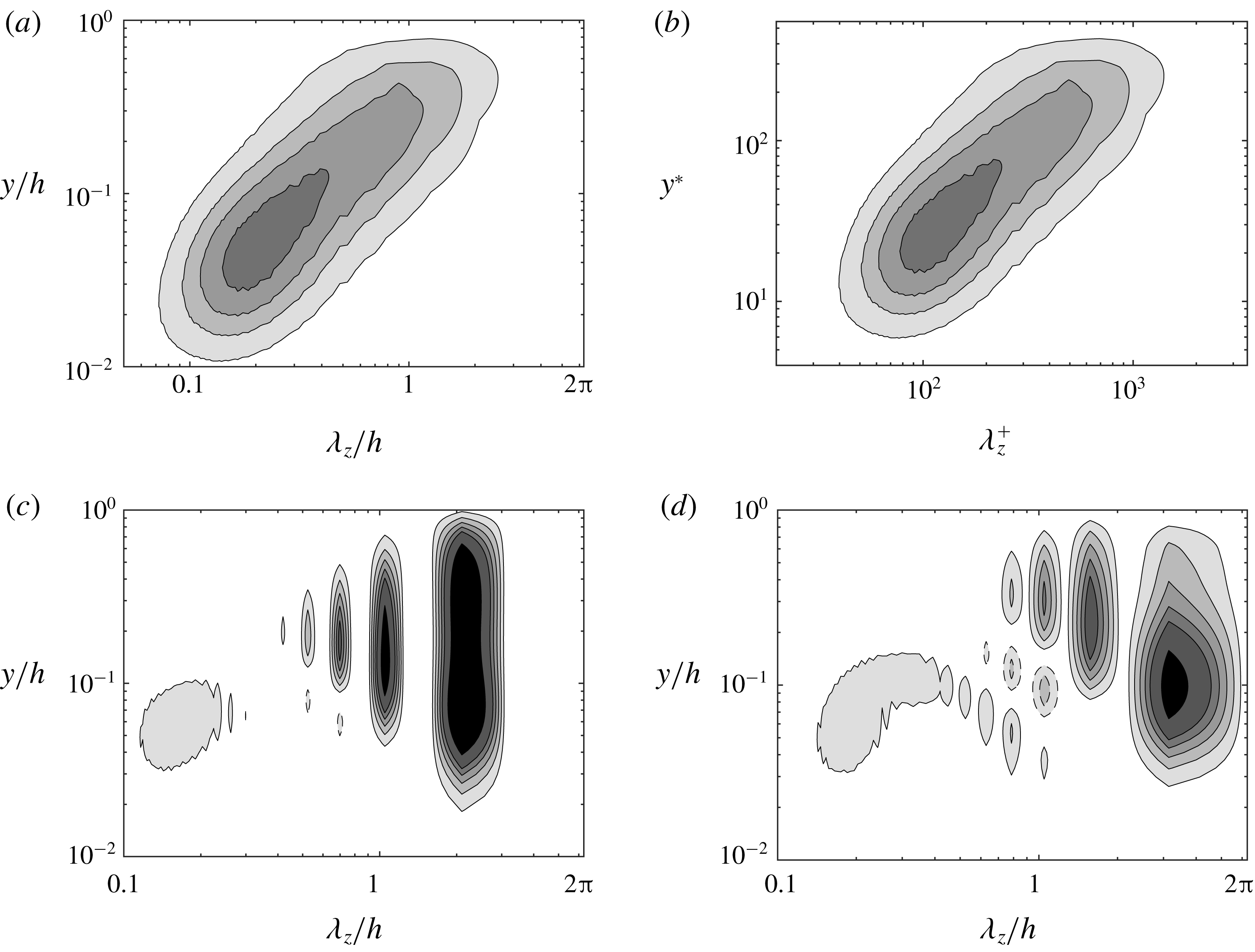
for the uncontrolled case is displayed in figure 9(a). For
 $Re_{\unicode[STIX]{x1D70F}}=180$
, it shows that the energy containing motions are mainly concentrated among
 $0.5\lesssim \unicode[STIX]{x1D706}/h\lesssim 1.1$
(or
 $100\lesssim \unicode[STIX]{x1D706}_{z}^{+}\lesssim 200$
) and
 $0.1\lesssim y/h\lesssim 0.3$
(or
 $20\lesssim y^{+}\lesssim 50$
) – these motions presumably correspond to quasi-streamwise vortices. This also explains the parametric study such that when setting
 $y_{c}^{+}$
within the buffer layer (figure 3
c), the energy containing motions are effectively weakened and hence significant drag reductions can be achieved. The effects of control at
 $A^{+}=0.015$
on the spanwise wavenumber spectrum of the total (
 $k_{z}\unicode[STIX]{x1D6F7}^{T}$
) and coherent (
 $k_{z}\unicode[STIX]{x1D6F7}^{C}$
) Reynolds shear stresses are shown in figure 9(b,c), respectively. The difference of the two spectra represents the random turbulent contribution (
 $k_{z}\unicode[STIX]{x1D6F7}^{R}$
), which is induced mostly by the near-wall small-scale motions (
 $y<0.3h$
and
 $\unicode[STIX]{x1D706}_{z}<2h$
). It is obvious that the contribution to the total Reynolds stress is mainly due to the coherent motions, consistent with figure 8(a). Compared with the uncontrolled case, the contribution from the near-wall region is effectively suppressed; the energy containing part is shifted outward, while
 $\unicode[STIX]{x1D706}_{z}$
is also changed from
 $0.5h$
to approximately
 $3h$
, the latter being close to the spacing of two adjacent control swirls. This suppression of structures at small scales is consistent with the observations of de Giovanetti, Sung & Hwang (Reference de Giovanetti, Sung and Hwang2017) in their study of streak instability for large-scale motions. Note that, as the forcing amplitude increases to
 $A^{+}=0.06$
, figure 9(c,d) shows that the Reynolds stress due to the coherent part (located in the outer region) further increases, while that from the random part is very small. Interestingly, there appears a positive Reynolds shear stress region (i.e.
 $1<\unicode[STIX]{x1D706}_{z}/h<2$
) marked by the dashed contours in figure 9(d,e), which actually results from the notable fluctuations in the Q1
 $(u^{\prime }>0,v^{\prime }>0)$
and Q3
 $(u^{\prime }<0,v^{\prime }<0)$
quadrants shown by the instantaneous velocity field in figure 11(f).
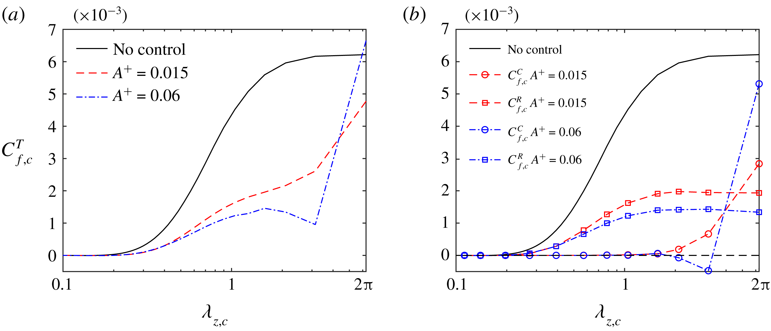
Cumulative friction coefficient of
 $C_{f,c}^{T}$
in (a), and of its coherent
 $C_{f,c}^{C}$
and random part
 $C_{f,c}^{C}$
in (b), varying with the cutoff spanwise wavelength
 $\unicode[STIX]{x1D706}_{z,c}$
. Note that the laminar part is subtracted from all of the plots.

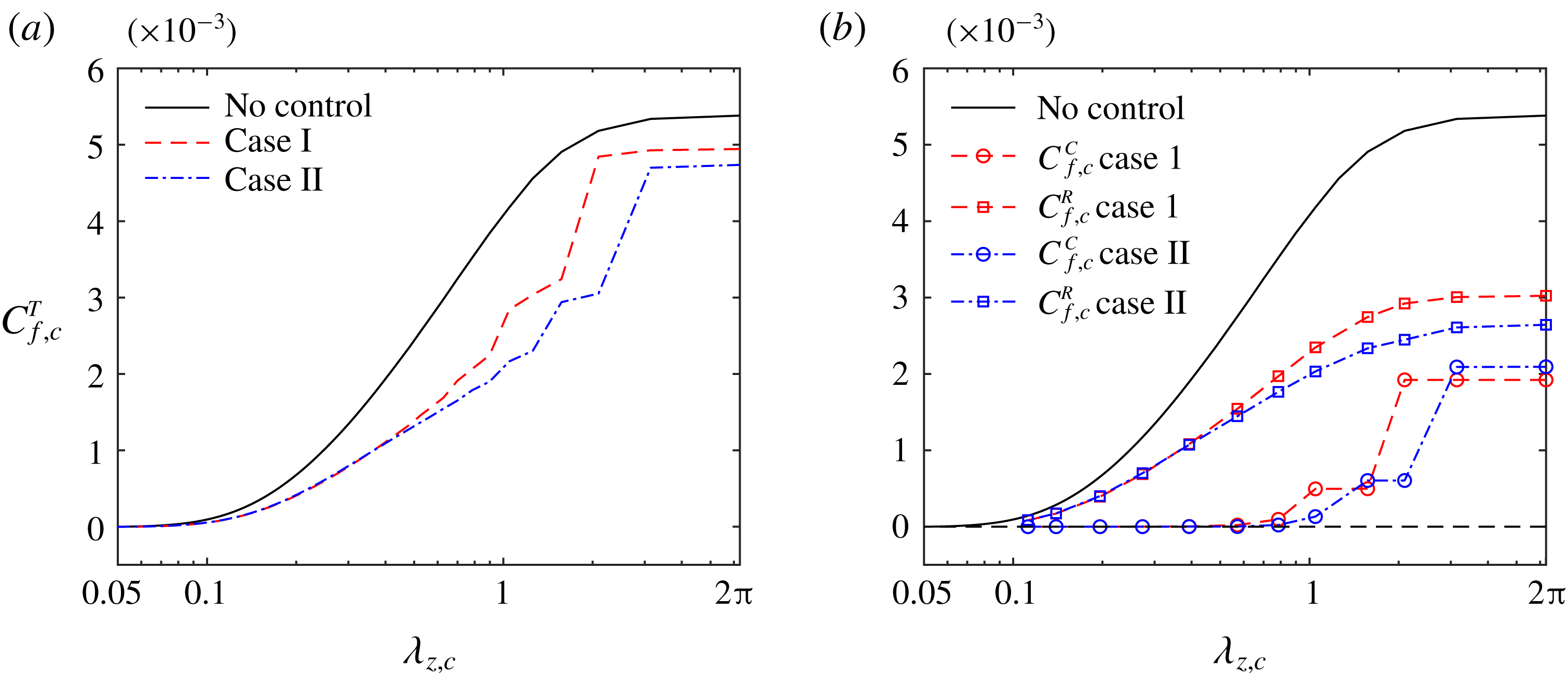
Finally, figure 10 shows the cumulative skin friction due to the turbulent motions of
 $\unicode[STIX]{x1D706}_{z}<\unicode[STIX]{x1D706}_{z,c}$
for different
 $A^{+}$
values. The laminar part, identical for all cases, is subtracted from the plot so that all of the cumulative
 $C_{f}$
values start from zero. For the uncontrolled case, motions with a spanwise scale in the range of
 $0.5h\leqslant \unicode[STIX]{x1D706}_{z}\leqslant 1.5h$
are responsible for the majority of the drag (approximately
 $54\,\%$
), consistent with the observation by de Giovanetti et al. (Reference de Giovanetti, Hwang and Choi2016). For controlled cases, the cumulative
 $C_{f}$
contributed by the total Reynolds stress is plotted in figure 10(a), and that by the coherent and random Reynolds stresses are plotted in figure 10(b). Taking
 $A^{+}=0.015$
in figure 10(b) for example, the random Reynolds shear stress is mainly induced by small-scale motions (
 $\unicode[STIX]{x1D706}_{z}<2h$
) and contributes to approximately 20 % of the total drag. In contrast, the coherent part is negligible for
 $\unicode[STIX]{x1D706}_{z}<2h$
and becomes important only when
 $\unicode[STIX]{x1D706}_{z}>2h$
, beyond which the random part is almost unchanged, and the coherent part alone contributes to the total cumulative drag increase. In this case, the effect of suppressing the small scales exceeds that of enhancing the large scales, leading to net drag decrease. As
 $A^{+}$
increases to
 $0.06$
, the random turbulent part due to the small scales further decreases. Note particularly the dip of the coherent part near
 $\unicode[STIX]{x1D706}_{z}\approx 2h$
is due the positive Reynolds shear stress identified in figure 9(e). Above this wavelength, the cumulative drag increases again due to the increasing contribution from the large-scale coherent motions. Thus, opposite to the
 $A^{+}=0.015$
case, the effect of excitation of the large scales at
 $A^{+}=0.06$
exceeds that of weakening the small-scale motions, hence leading to net drag increase.
4.3 Coherent structures
Contour of streamwise velocity fluctuations in the (
 $x{-}z$
) plane at
 $y^{\ast }=20$
: (a) no control; (b)
 $u^{\prime }$
for
 $A^{+}=0.015$
; (c)
 $u^{\prime \prime }$
for
 $A^{+}=0.015$
; (d)
 $u^{\prime }$
for
 $A^{+}=0.06$
; and (e)
 $u^{\prime \prime }$
for
 $A^{+}=0.06$
. The forcing spacing is
 $\unicode[STIX]{x1D706}^{+}=360\unicode[STIX]{x03C0}$
and control height is
 $y_{c}^{+}=30$
.

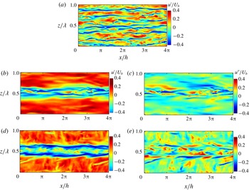
Figure 11 shows the contours of the low-speed streaks for both
 $u^{\prime }$
and
 $u^{\prime \prime }$
at
 $y^{\ast }=20$
for different forcing amplitudes (uncontrolled
 $A^{+}=0$
, low
 $A^{+}=0.015$
and high
 $A^{+}=0.06$
). While typical meandering low-speed streaky structures are observed aligned along the streamwise direction in the uncontrolled case (figure 11
a), the number of streaks is decreased for the controlled cases. In the presence of control, the basic near-wall streaks of
 $u^{\prime }$
are destroyed (figure 11
b,d), and the near-wall flow becomes a single very wide meandering streak extending the entire flow length, as expected from the merger of the numerous background streaks forced by the two wall jets. Note that such a widening and weakening of near-wall streaks has also been found in the drag reduction by spanwise wall oscillations (Jung et al.
Reference Jung, Mangiavacchi and Akhavan1992; Akhavan, Jung & Mangiavacchi Reference Akhavan, Jung and Mangiavacchi1993), which presumably plays a similar role as SOJF merging many streaks together. The streaks are located essentially in the collision region – particularly clear in the random part
 $u^{\prime \prime }$
(figure 11
c) when the coherent flow
 $\tilde{u}$
is subtracted from the total fluctuation velocity
 $u^{\prime }$
. As the forcing amplitude increases, more random streaks appear (figure 11
e), which is consistent with the greater number of vortical structures observed in figure 13(e).
Vector plots of
 $(v,w)$
in the (
 $y{-}z$
) plane located at
 $x=L_{x}/3$
: (a) no control; (b)
 $A^{+}=0.015$
; and (c)
 $A^{+}=0.06$
. Light (yellow) and dark (blue) colours indicate positive and negative streamwise velocity fluctuations
 $u^{\prime }$
. The forcing spacing is
 $\unicode[STIX]{x1D706}^{+}=360\unicode[STIX]{x03C0}$
and control height is
 $y_{c}^{+}=30$
.

Iso-surfaces of
 $\unicode[STIX]{x1D706}_{2}=-1$
(shaded with the wall-normal distance from the bottom wall): (a) no control; (c)
 $\unicode[STIX]{x1D706}^{+}=360\unicode[STIX]{x03C0}$
and
 $A^{+}=0.015$
; (e)
 $\unicode[STIX]{x1D706}^{+}=360\unicode[STIX]{x03C0}$
and
 $A^{+}=0.06$
; (b,d) and (f) are the corresponding skin friction normalized by the uncontrolled case on the bottom wall.

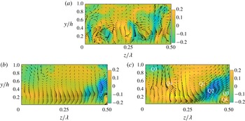
The flow field difference among the three different amplitudes is further examined through the velocity vectors in the cross-stream (
 $y{-}z$
) plane, in figure 12. Here, the light (yellow) colour indicates positive streamwise velocity fluctuation
 $u^{\prime }$
and dark (blue) colour indicates negative streamwise velocity fluctuation
 $u^{\prime }$
(only the left half-domain
 $z/\unicode[STIX]{x1D706}\leqslant 0.5$
is displayed, since the left and right parts are almost symmetric). Compared with the chaotic feature of the uncontrolled case (figure 12
a), the velocity vectors near the wall are more parallel along the spanwise direction for
 $A^{+}=0.015$
, indicating organized motions induced by SOJF similar to that of figure 5(a). Moreover, the downwash by the near-wall streamwise vortices observed in the uncontrolled case is significantly reduced by the SOJF. At higher
 $A^{+}=0.06$
, the control flow is clearly much more dominant and organized. As marked in figure 12(c), a strong Q2 event (negative
 $u^{\prime }$
and positive
 $v^{\prime }$
associated with the lift up of the large-scale swirls) occurs in the region
 $0.3\lesssim z/\unicode[STIX]{x1D706}\lesssim 0.5$
, contributing to the increase of Reynolds shear stress in the bulk flow (figure 8) and hence drag increment. In addition, notable Q1 and Q3 events are also observed (located between Q2 and Q4 events), which cause the alternative positive/negative Reynolds shear stress contours in figures 9(d,e).
We then display the
 $\unicode[STIX]{x1D706}_{2}$
vortices (Jeong & Hussain Reference Jeong and Hussain1995) (calculated based on the random turbulent fluctuation velocity
 $\boldsymbol{u}^{\prime \prime }$
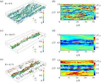
) and the skin friction at the bottom wall in figure 13. Note that numerous slender vortices are distributed throughout the wall region in the uncontrolled case (figure 13
a), lying directly above the high skin friction regions (figure 13
b); and hairpins are few and far between, consistent with the observations of Schlatter et al. (Reference Schlatter, Li, Örlü, Hussain and Henningson2014). At
 $A^{+}=0.015$
, most of the near-wall streamwise vortices disappear except near the collision region, just above the merged streak envelope (figure 13
c); this disappearance is consistent with the suppression of
 $\unicode[STIX]{x1D714}_{x,rms}^{\prime \prime }$
in figure 6(d). From figure 13, we observe that the vortex structures mostly lie on top of the low skin friction region, which would appear to contradict the well-accepted notion that peak skin friction underlines streamwise vortices. This apparent enigma is reconciled below.
(a,b) Cross-section view of the instantaneous
 $\unicode[STIX]{x1D706}_{2}$
structures; (c,d) low-speed streaks; and (e,f) spanwise distribution of the wall shear stress at streamwise location
 $x=L_{x}/3$
. Note that the dashed line in the bottom row is the streamwise- and time-averaged wall shear stress. The left and right columns are for
 $A^{+}=0.015$
; and
 $A^{+}=0.06$
, respectively.

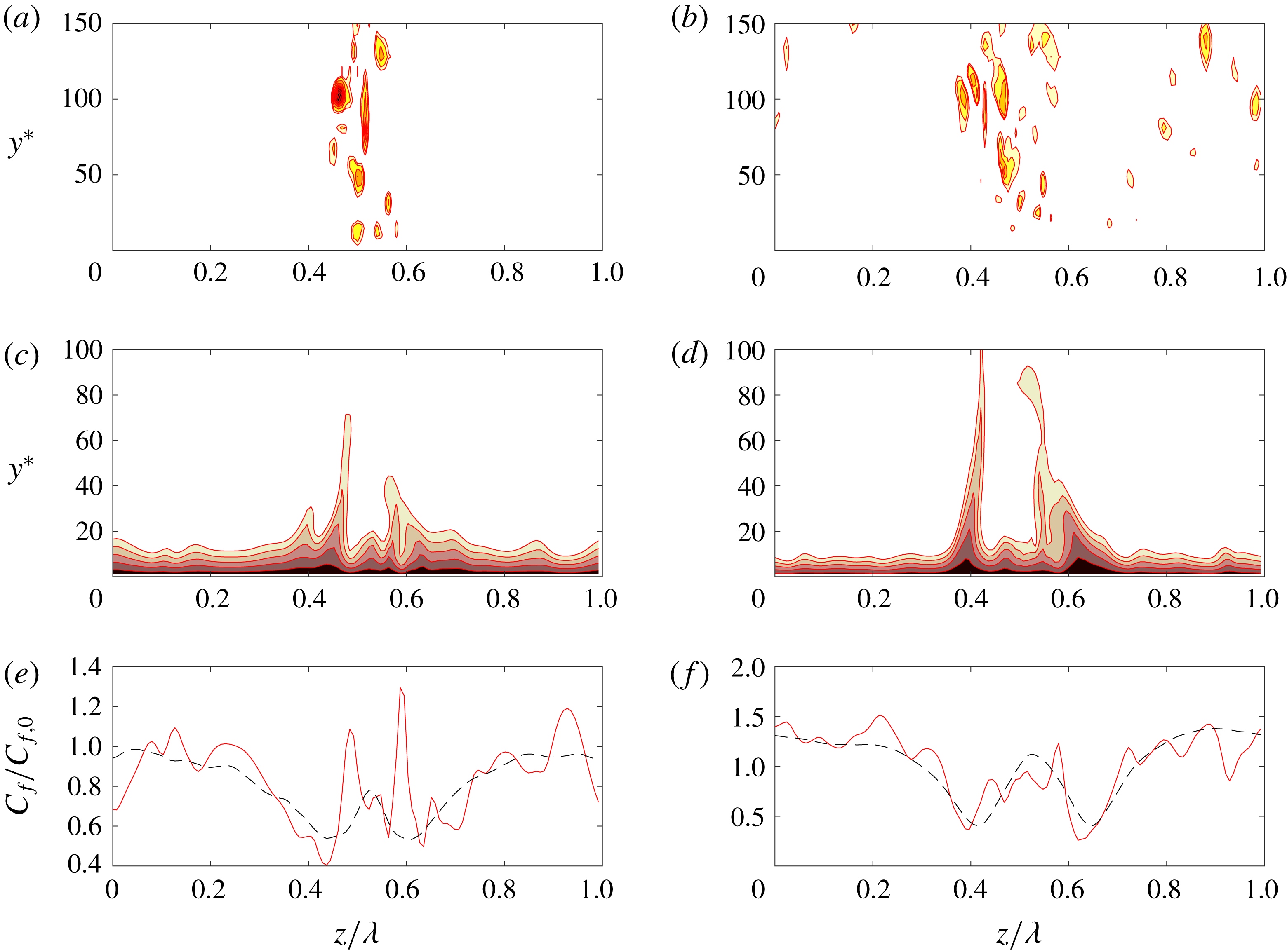
Figure 14 shows the instantaneous cross-section view of
 $\unicode[STIX]{x1D706}_{2}$
contours at a specific streamwise location
 $x=L_{x}/3$
, together with the associated low-speed streaks and the spanwise variation of wall shear stress. The strength of combined large streak envelope, although below the critical value, is so only on an average basis, some individual streaks survive on an instantaneous basis with very high flank angles (figure 14
c,d). Although it may not be obvious, instantaneously the vortical structures, the streaks and wall shear stress are quite uniquely related; there are instances and locations of high instantaneous wall shear stresses, which can be uniquely identified with instantaneous streamwise vortical structures. However, after ensemble averaging, the spiked wall shear stress is no longer apparent, due to the intermittent feature of these vortices.
Contours (red lines) of (a)
 $\unicode[STIX]{x1D714}_{x}$
; (b) forcing generation; (c) the
 $-\unicode[STIX]{x2202}_{x}w\unicode[STIX]{x2202}_{y}u$
(wall-normal vorticity) tilting; (d) the
 $\unicode[STIX]{x2202}_{x}v\unicode[STIX]{x2202}_{z}u$
(spanwise vorticity) tilting; (e) vortex stretching; (f) the cross-stream (
 $y{-}z$
) advection. The dash line in (a) indicates the low-speed streak in figure 14(a); (b–f) identify the positive
 $\unicode[STIX]{x1D714}_{x}$
boundaries as shown in (a). Also in (a–f), solid (dot-dashed) lines indicate positive (negative) magnitudes of each term.

The above investigation triggers another important question, i.e. where do these vortical structures above the streak envelope come from? Do they get pushed outward from the wall or freshly created locally? Note that since the vortices are predominantly streamwise (figure 13
c), the evolutionary dynamics of
 $\unicode[STIX]{x1D714}_{x}$
is further investigated here. The inviscid evolution of
 $\unicode[STIX]{x1D714}_{x}$
is governed by
 $$\begin{eqnarray}\displaystyle \frac{\unicode[STIX]{x2202}\unicode[STIX]{x1D714}_{x}}{\unicode[STIX]{x2202}t}=\underbrace{\unicode[STIX]{x1D714}_{x}\frac{\unicode[STIX]{x2202}u}{\unicode[STIX]{x2202}x}}_{\text{I}}-\underbrace{\frac{\unicode[STIX]{x2202}w}{\unicode[STIX]{x2202}x}\frac{\unicode[STIX]{x2202}u}{\unicode[STIX]{x2202}y}}_{\text{IIa}}+\underbrace{\frac{\unicode[STIX]{x2202}v}{\unicode[STIX]{x2202}x}\frac{\unicode[STIX]{x2202}u}{\unicode[STIX]{x2202}z}}_{\text{IIb}}-\underbrace{u\frac{\unicode[STIX]{x2202}\unicode[STIX]{x1D714}_{x}}{\unicode[STIX]{x2202}x}}_{\text{III}}-\underbrace{v\frac{\unicode[STIX]{x2202}\unicode[STIX]{x1D714}_{x}}{\unicode[STIX]{x2202}y}-w\frac{\unicode[STIX]{x2202}\unicode[STIX]{x1D714}_{x}}{\unicode[STIX]{x2202}z}}_{\text{IV}}+\underbrace{\frac{\unicode[STIX]{x2202}F_{z}}{\unicode[STIX]{x2202}y}}_{\text{V}}. & & \displaystyle\end{eqnarray}$$
The terms on the right-hand side are: (I) vortex stretching, (IIa,b) vortex tilting, (III) streamwise advection, (IV) cross-stream advection and (V) vorticity generation due to forcing.
In order to get some clear understanding of the flow physics, it is necessary to evaluate the role of each term in the vorticity equation (4.8). Note that for simplicity, we focus on the structures with positive streamwise vorticity
 $+\unicode[STIX]{x1D714}_{x}$
(SP) and their generation, ignoring the comparable numbers of negative streamwise vorticity
 $-\unicode[STIX]{x1D714}_{x}$
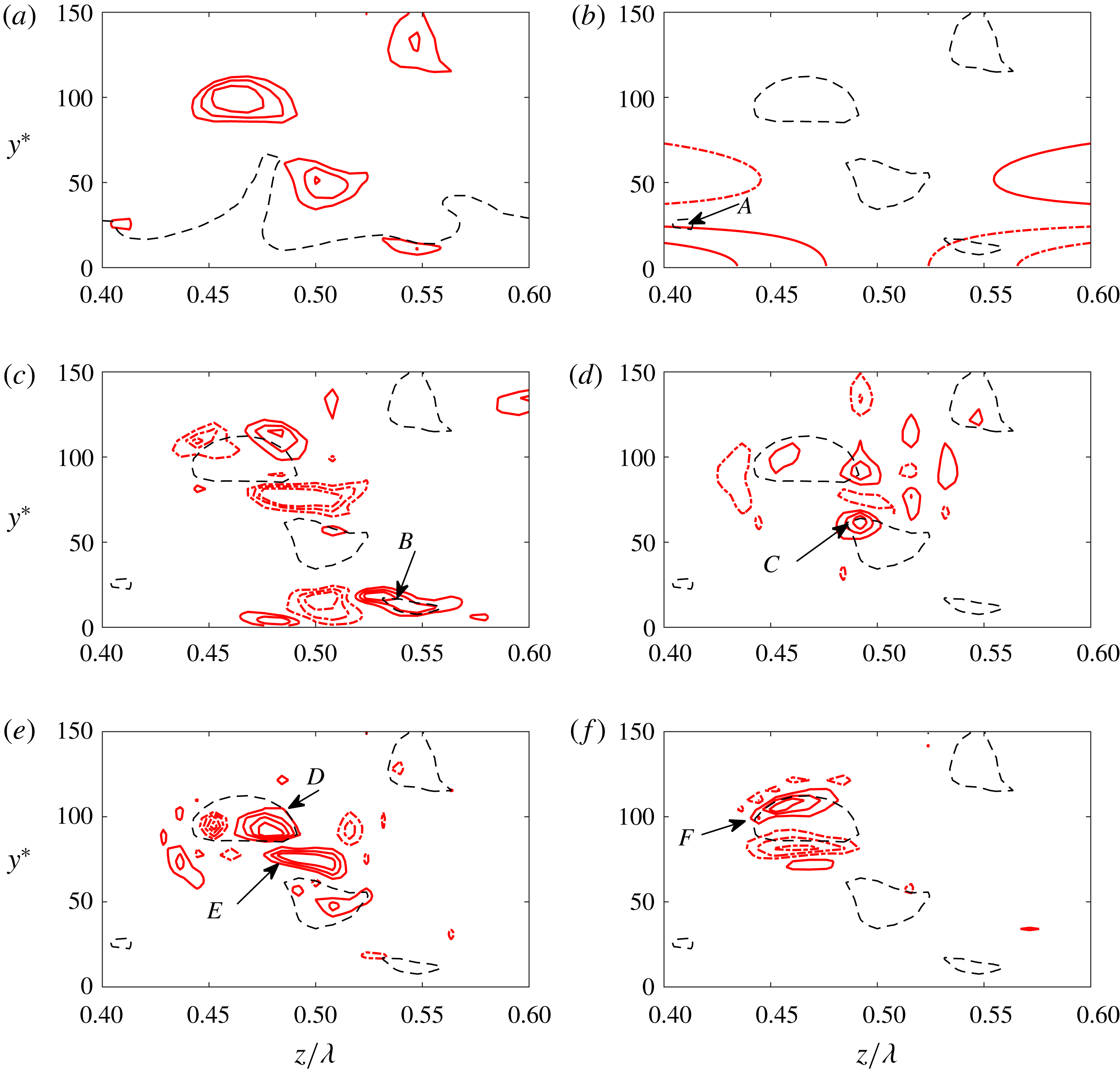
(SN) structures. Figure 15 shows a small domain around the mid-span of figure 14: (a)
 $\unicode[STIX]{x1D714}_{x}$
associated with SPs, along with the low-speed streak boundary from figure 14(c); (b)
 $\unicode[STIX]{x1D714}_{x}$
generation by the forcing term (V); (c)
 $\unicode[STIX]{x1D714}_{x}$
generation by wall-normal vorticity titling (
 $-\unicode[STIX]{x2202}_{x}w\unicode[STIX]{x2202}_{y}u$
, IIa); (d)
 $\unicode[STIX]{x1D714}_{x}$
generation by spanwise vorticity titling (
 $\unicode[STIX]{x2202}_{x}v\unicode[STIX]{x2202}_{z}u$
, IIb); (e) streamwise vortex stretching (I); and (f) cross-stream advection (IV). Note that the key
 $+\unicode[STIX]{x1D714}_{x}$
contours (SP structures) from figure 15(a) are repeated in figures 15(b–f) in order to provide a common spatial reference. Generation terms which strengthen SP are indicated by positive values (solid lines), while negative values indicate local weakening of SP (dash-dot lines).
At location
 $A$
in figure 15(b), one SP is generated by the shearing induced by forcing. Most of the SPs are located in the middle region (
 $z/\unicode[STIX]{x1D706}\sim 0.5$
), where the forcing generation term is small. The source of generation of these SPs with
 $+\unicode[STIX]{x1D714}_{x}$
is mainly the tilting of spanwise and wall-normal vorticity by the streamwise flow induced shear. For example, in the near-wall region (
 $y^{\ast }<50$
,
 $B$
in figure 15
c), we find important vorticity generation due to the wall-normal vorticity tilting
 $-\unicode[STIX]{x2202}_{x}w\unicode[STIX]{x2202}_{y}u$
by the streamwise flow, where the instantaneous streak has a steep flank
 $\unicode[STIX]{x1D714}_{y}$
(figure 15
c). In the bulk flow (at point
 $C$
in figure 15
d where
 $y^{\ast }\sim 50$
), the spanwise vorticity tilting by streamwise velocity enhances the SP due to the presence of highly lifted-up low-speed streak (having strong
 $\unicode[STIX]{x2202}_{z}u$
). Note that once SPs are generated, they are further amplified by the direct stretching due to the streak waviness
 $\unicode[STIX]{x2202}_{x}u$
(similar to that observed by SH1), evident from the strong regions of
 $+\unicode[STIX]{x1D714}_{x}\unicode[STIX]{x2202}_{x}u$
embedded in SP (region
 $D$
in figure 15
e). Note that the intense vortex stretching (producing
 $+\unicode[STIX]{x1D714}_{x}$
at point
 $E$
in figure 15
e), does not result in SP, due to the simultaneous counter-effect of the tilting (producing
 $-\unicode[STIX]{x1D714}_{x}$
) in figure 15(c). Finally, the generated SP structures are further transported outward by the swirls as also downstream by the base flow, evident from the positive amplitude of the advection term on top of the SP in
 $F$
in figure 15(f).
For the higher forcing amplitude
 $A^{+}=0.06$
case, the skin friction near the wall-jet sides is significantly increased (figure 14
f) due to the squashing of the wall jet, and hence increased
 $\unicode[STIX]{x2202}u/\unicode[STIX]{x2202}y$
(figure 11
f). Although numerous streaks merge into a large streak envelope, the streak strength is larger near the collision plane (figure 14
d) compared with the small amplitude case
 $A^{+}=0.015$
, and hence leads to the generation of more vortex structures, as seen in figure 14(b). In addition, the downwash of the secondary swirls is larger and stronger at high
 $A^{+}$
(i.e.
 $=0.06$
), which causes a local high skin friction at the mid-span (i.e.
 $z/\unicode[STIX]{x1D706}\approx 0.5$
in figure 14
f).
4.4 The effect of
$y_{c}^{+}$

Cross-stream (
 $y{-}z$
) plane view of (a) mean velocity field (
 $\overline{\boldsymbol{u}}$
) with the contours indicating the mean streamwise velocity (normalized by
 $U_{b}$
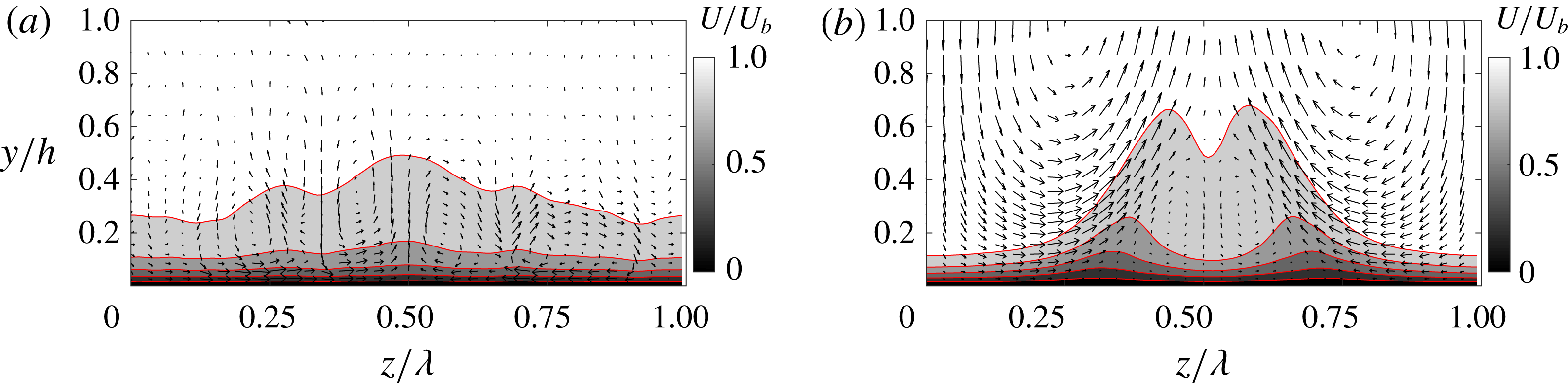
), and the vectors denoting the wall-normal and spanwise velocities for (a)
 $y_{c}^{+}=5$
; (b)
 $y_{c}^{+}=80$
.

Compared with the previous large-scale control methods (Canton et al.
Reference Canton, Örlü, Chin, Hutchins, Monty and Schlatter2016a
, SH2), where the height of the control swirl was fixed at the centre of the channel, a major difference of the current SOJF method is the introduction of
 $y_{c}$
to characterize the wall-jet height. To demonstrate the effect of
 $y_{c}^{+}$
on drag reduction
 ${\mathcal{R}}$
, two additional cases with
 $y_{c}^{+}=5$
and
 $80$
are discussed here (while
 $A^{+}=0.015$
and
 $\unicode[STIX]{x1D706}^{+}=360\unicode[STIX]{x03C0}$
remain the same as the optimal for
 $y_{c}^{+}=30$
). Compared with the case at
 $y_{c}^{+}=30$
(producing
 $18.6\,\%\pm 0.9\,\%$
of
 ${\mathcal{R}}$
),
 ${\mathcal{R}}$
becomes
 $1.4\,\%\pm 0.7\,\%$
and
 $13.5\,\%\pm 1.1\,\%$
for
 $y_{c}^{+}=5$
and
 $80$
, respectively. Figure 16 shows the cross-streamwise view (the (
 $y{-}z$
) plane) of contours of the streamwise velocity and the cross-plane velocity vectors of
 $\overline{\boldsymbol{u}}$
for the two different forcing height cases. For the low
 $y_{c}^{+}$
case, the wall jet is too thin, and limited very close to the bottom wall, which hardly has any effect on the suppression of the streaks, whilst at high
 $y_{c}^{+}$
, the energetic, counter-rotating swirls well organize the flow, and the squashing effect along the sides of the swirls also becomes stronger. Compared to
 $y_{c}^{+}=30$
, the secondary swirls at
 $y_{c}^{+}=80$
near the collision plane are much larger, separating the dual peaks further.
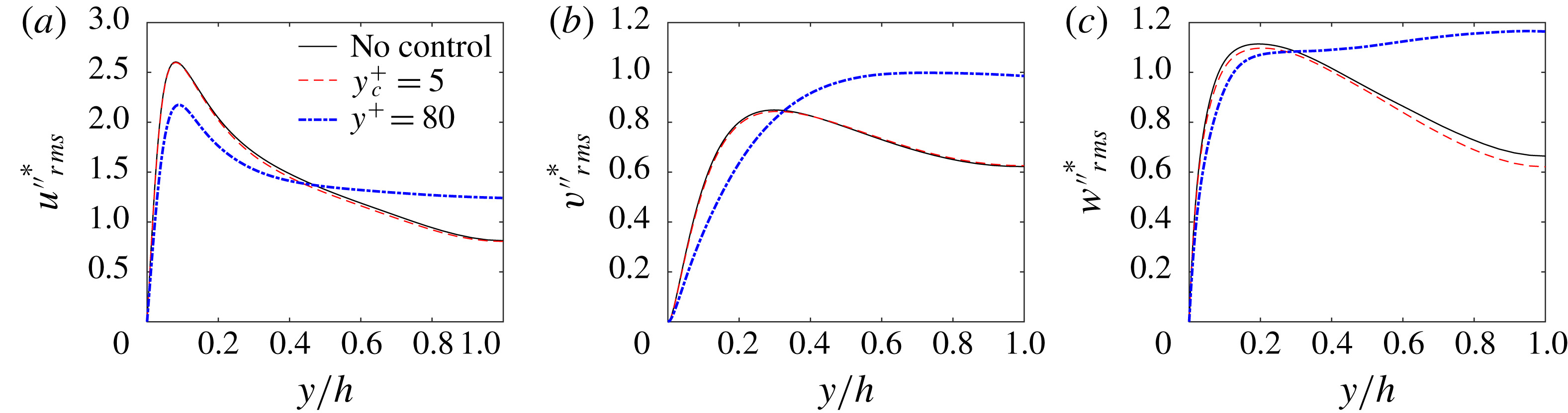
Figure 17 further shows the spanwise-averaged turbulent fluctuations
 $\{\langle \overline{u_{i}^{\prime \prime 2}}\rangle ^{1/2}\}^{\ast }$
. For
 $y_{c}^{+}=5$
, turbulent fluctuations are almost unchanged, as extremely near-wall forcing is ineffective, as discussed above, also consistent with figure 8(b) where
 $C_{f}^{C}$
is rather small and
 $C_{f}^{T}$
is nearly unchanged. For
 $y_{c}^{+}=80$
, the turbulent fluctuations are suppressed near the wall (due to the merger of streaks), while they are increased in the outer flow region (due to upward advecting of the structures). Since coherent motions are more pronounced at
 $y_{c}^{+}=80$
compared to
 $y_{c}^{+}=5$
(figure 16), a larger
 $C_{f}^{C}$
is observed for
 $y_{c}^{+}=80$
, as shown in figure 8(b).
 $C_{f}^{C}$
is also
 $5\,\%$
larger at
 $y_{c}^{+}=80$
compared to that of
 $y_{c}^{+}=30$
, leading to the degradation of
 ${\mathcal{R}}$
as
 $y_{c}^{+}$
increases.
Spanwise-averaged turbulent velocity fluctuations for various forcing heights
 $y_{c}^{+}$
at
 $A^{+}=0.015$
and
 $\unicode[STIX]{x1D706}^{+}=360\unicode[STIX]{x03C0}$
.

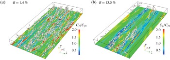
Iso-surfaces of
 $\unicode[STIX]{x1D706}_{2}=-1$
associated with the contours of the corresponding skin friction on the bottom walls normalized by the uncontrolled case: (a)
 $y_{c}^{+}=5$
; (b)
 $y_{c}^{+}=80$
at
 $Re_{\unicode[STIX]{x1D70F}}=180$
.

Similar to figure 13, the
 $\unicode[STIX]{x1D706}_{2}$
vortex and the corresponding skin friction at the bottom wall are displayed in figure 18 for
 $y_{c}^{+}=5$
and
 $80$
. It is obvious that the near-wall structures are barely suppressed at
 $y_{c}^{+}=5$
compared with the uncontrolled case. At
 $y_{c}^{+}=80$
, much fewer vortex structures survive near the mid-span. In addition, there are two distinct low skin friction regions lying along the streamwise direction, caused by the near-wall lifting up and separated by the larger secondary swirls. The downwash motions associated with the larger secondary swirls would cause drag increase and should be suppressed also. In summary, it is clear that
 $y_{c}$
has to have an optimal value – neither too small nor too large.
5 Discussion
5.1 Power performance
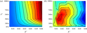
Map of (a) the power spent
 $P_{in}/P_{0}$
(%) and (b) net power saving
 ${\mathcal{N}}$
(%) as a function of
 $A^{+}$
and
 $\unicode[STIX]{x1D706}^{+}$
for
 $y_{c}^{+}=30$
at
 $Re_{\unicode[STIX]{x1D70F}}=180$
.

Active control techniques are evaluated not only by
 ${\mathcal{R}}$
, but also by the net power saving
 ${\mathcal{N}}$
, subtracting the energy cost of the control. The value of
 ${\mathcal{N}}$
, in a turbulent channel flow, is defined as
 $$\begin{eqnarray}\displaystyle {\mathcal{N}}={\mathcal{R}}-P_{in}/P_{0}, & & \displaystyle\end{eqnarray}$$
where
 $P_{0}$
is the power required to drive the uncontrolled flow, and
 $P_{in}$
is the control input power, calculated as
 $\int _{\unicode[STIX]{x1D6FA}}\boldsymbol{f}\boldsymbol{\cdot }\tilde{\boldsymbol{u}}\,\text{d}\unicode[STIX]{x1D6FA}$
by neglecting the electro-mechanical losses of a real actuator (Canton et al.
Reference Canton, Örlü, Chin and Schlatter2016b
; Mahfoze & Laizet Reference Mahfoze and Laizet2017).
Figure 19(a,b) presents the energy input
 $P_{in}/P_{0}$
and the net power
 ${\mathcal{N}}$
as a function of
 $A^{+}$
and
 $\unicode[STIX]{x1D706}^{+}$
at
 $y^{+}=30$
. The energy input, quite small for small
 $A^{+}$
, increases as
 $A^{+}$
and
 $\unicode[STIX]{x1D706}^{+}$
increase. In particular,
 $P_{in}/P_{0}$
is only approximately
 $2.1\,\%$
for our optimal drag reduction case. From figure 19(b), it is obvious that the contour of net power saving is qualitatively similar to that of
 ${\mathcal{R}}$
shown in figure 2. It is encouraging to note that there is a wide range of control parameters yielding positive net power rates. The value of
 ${\mathcal{N}}$
for the optimal case (
 $A^{+}=0.015$
and
 $\unicode[STIX]{x1D706}^{+}=360$
) is approximately
 $16.5\,\%$
. Although this high net power saving is impressive, note that the value is based on a simple estimation of the actuation, where actuator’s energy transfer efficiency has not been addressed. For real applications, it is known that currently many actuators suffer from a quite low energy transfer efficiency, i.e. around 1 % from electrical power to mechanical power for plasma-based actuators (Erfani et al.
Reference Erfani, Zare-Behtash, Hale and Kontis2015; Mahfoze & Laizet Reference Mahfoze and Laizet2017).
5.2 Control efficacy at higher
$Re$

Another important issue for drag control methods is the performance at high
 $Re$
. As shown in Yao et al. (Reference Yao, Chen, Thomas and Hussain2017), for given values of
 $y_{c}^{+}=30$
,
 $\unicode[STIX]{x1D706}^{+}\approx 1200$
and
 $A^{+}\approx 0.015$
,
 ${\mathcal{R}}$
shows a gradual variation with
 $Re$
-dependence. The degradation of
 ${\mathcal{R}}$
with increasing
 $Re$
has also been observed in other control strategies, such as spanwise wall oscillations (Quadrio Reference Quadrio2011; Gatti & Quadrio Reference Gatti and Quadrio2013, Reference Gatti and Quadrio2016) and the blow/suction method (Chung & Talha Reference Chung and Talha2011). The reason seems to be the failure to control of the energetic large-scale structures at the high
 $Re$
(de Giovanetti et al.
Reference de Giovanetti, Hwang and Choi2016), which has also been explained in Gatti & Quadrio (Reference Gatti and Quadrio2016) based on the upward shift of the viscous sublayer.
Drag reduction rate
 ${\mathcal{R}}$
(
 $\%$
) at
 $Re_{\unicode[STIX]{x1D70F}}=550$
as a function of
 $A^{+}$
and
 $\unicode[STIX]{x1D706}^{+}$
for (a)
 $y_{c}^{+}=30$
; (b)
 $y_{c}^{+}=50$
.

Cross-stream (
 $y{-}z$
) plane view of (a) mean velocity field (
 $\overline{\boldsymbol{u}}$
) for one control wavelength with the contours indicating the mean streamwise velocity (normalized by
 $U_{b}$
), and the vectors denoting the wall-normal and spanwise velocities for (a) case I; (b) case II; (c) the associated spanwise distribution of the wall shear stress normalized with the uncontrolled case.

To better understand the
 $Re$
dependence of our method, a limited parametric study is performed at
 $Re_{\unicode[STIX]{x1D70F}}=550$
(with
 $y_{c}^{+}$
range from
 $30,50$
to
 $70$
,
 $\unicode[STIX]{x1D706}^{+}$
from
 $550\unicode[STIX]{x03C0}/3$
to
 $1100\unicode[STIX]{x03C0}$
and
 $A^{+}$
from
 $0.012$
to
 $0.024$
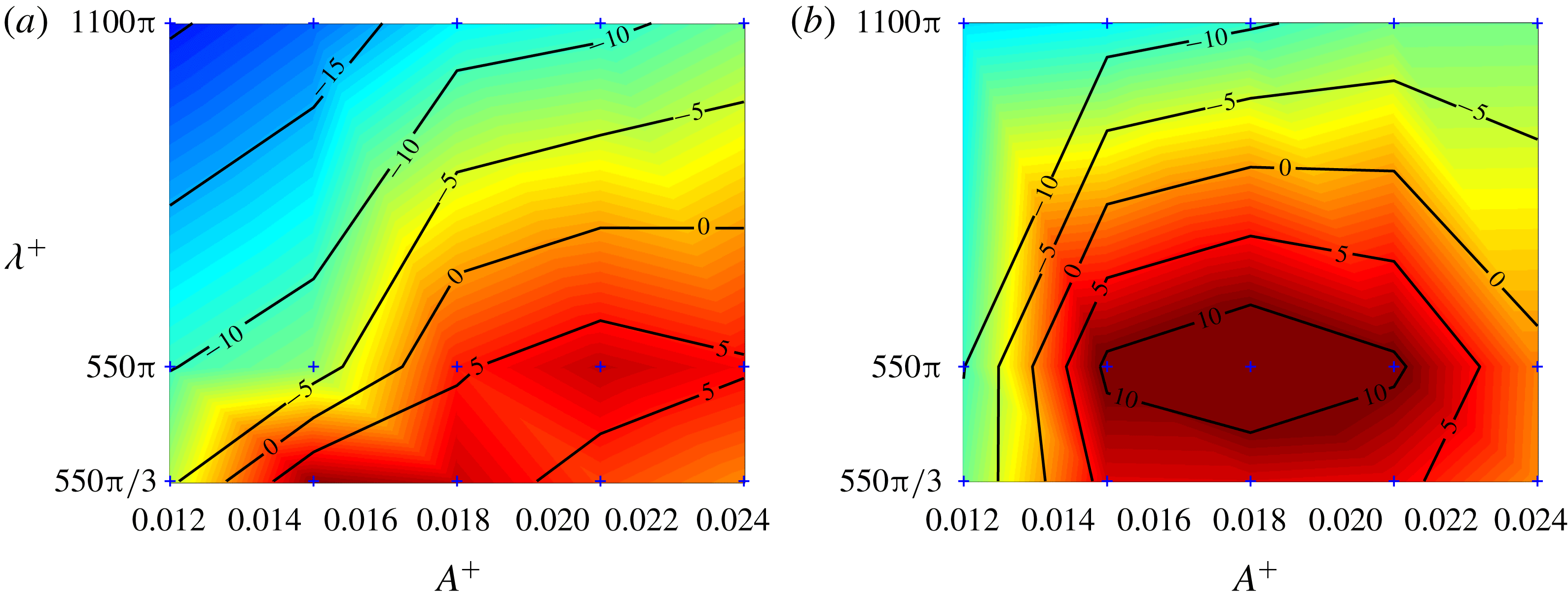
). Figure 20(a) shows the drag reduction
 ${\mathcal{R}}$
as a function of
 $A^{+}$
and
 $\unicode[STIX]{x1D706}^{+}$
at
 $y_{c}^{+}=30$
. Compared with
 $Re_{\unicode[STIX]{x1D70F}}=180$
(figure 2), there is a moderate deterioration in
 ${\mathcal{R}}$
. In particular, keeping the parameters same as found optimal at
 $Re_{\unicode[STIX]{x1D70F}}=180$
, namely,
 $\unicode[STIX]{x1D706}^{+}\approx 1200$
,
 $A^{+}\approx 0.015$
and
 $y_{c}^{+}=30$
(denoted as case I),
 ${\mathcal{R}}$
decreases from
 $18.6\,\%\pm 0.9\,\%$
to
 $10.2\,\%\pm 0.8\,\%$
as
 $Re_{\unicode[STIX]{x1D70F}}$
increases from
 $180$
to
 $550$
(note that a 2 % difference for
 $Re_{\unicode[STIX]{x1D70F}}=550$
reported in Yao et al. (Reference Yao, Chen, Thomas and Hussain2017) is due to a smaller box size used there). It does not necessarily imply that our method is less effective at high
 $Re$
. Because of the strong dependence of
 ${\mathcal{R}}$
on the choice of forcing parameters, the drag reduction drop might be less pronounced in certain ranges of controlling parameters. For example, figure 20 shows that the forcing using
 $y_{c}^{+}=50$
is superior to that with
 $y_{c}^{+}=30$
– over a wide range with notable
 ${\mathcal{R}}$
. A high
 ${\mathcal{R}}$
of
 $14.5\,\%\pm 0.8\,\%$
is achieved with slightly larger parameters
 $A^{+}=0.018$
,
 $\unicode[STIX]{x1D706}^{+}=1728$
and
 $y_{c}^{+}=50$
(denoted as case II). Different from previous near-wall drag control methods where the optimal parameters typically scale in wall units, the optimal control parameters of our large-scale SOJF method, to accommodate the outer shifted energy containing motions, seem to follow a mixed scaling. While
 $y_{c}^{+}$
increasing moderately with
 $Re$
seems to follow the peak location of the Reynolds shear stress (see Xi, Hussain & She Reference Xi, Hussain and She2018), the control wavelength may scale in outer units – to be validated at higher
 $Re$
simulations in the future.
Iso-surfaces of
 $\unicode[STIX]{x1D706}_{2}=-1$
associated with the contours of the corresponding skin friction on the bottom walls normalized by the uncontrolled case: (a) uncontrolled; (b) case I; (c) case II. Note that the right column shows the zoomed views of the region marked on the left panel.

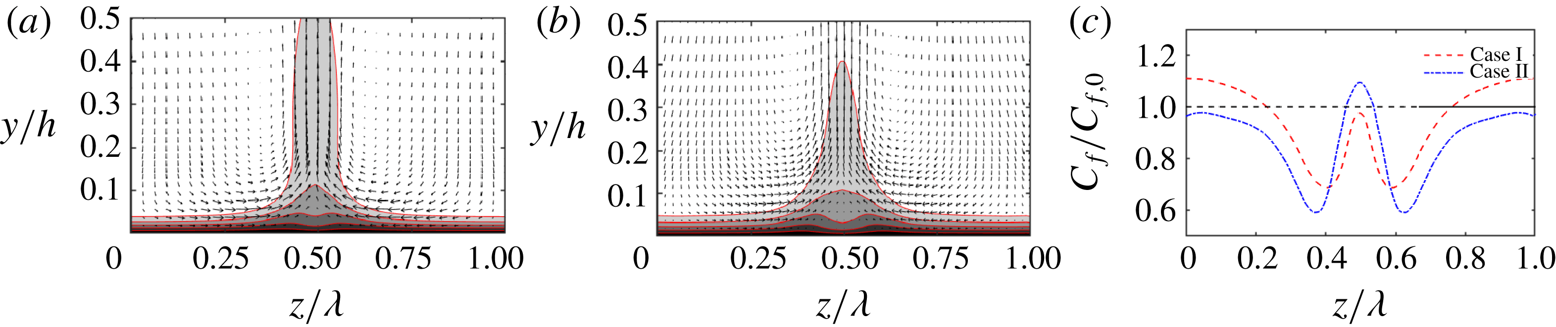
To explain how this additional drag is achieved, flow field alterations by controls are examined. Figure 21 shows the cross-streamwise view of contours of the streamwise velocity and the cross-plane velocity vectors of
 $\overline{\boldsymbol{u}}$
. Again, both cases clearly show the merged streak envelope, and the downwash motions between the large-scale swirls cause a dual peak of streak envelope near the wall, as well as a relatively high skin friction near the collision region compared to case I, which shows drag increase near the two sides of the swirls due to a small
 $\unicode[STIX]{x1D706}^{+}$
, case II produces smaller skin friction near the two sides, due to the smaller squashing effect observed in figure 21(b). Figure 22 shows the
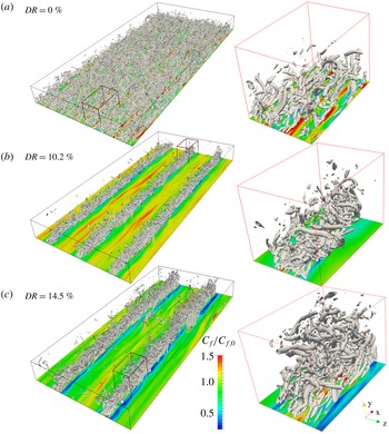
 $\unicode[STIX]{x1D706}_{2}$
structures and skin friction distribution at the bottom wall. The vortical structures typically show a similar pattern as in the optimal case at
 $Re_{\unicode[STIX]{x1D70F}}=180$
(albeit the structures are far more numerous and packed in the high
 $Re$
case): most of the vortices are eliminated except near the swirl collision region. Thus, it confirms that, at
 $Re_{\unicode[STIX]{x1D70F}}=550$
, SOJF can successfully produce drag reduction through the merger of streaks, hence suppressing the vortical structures. Also note that a slight difference in vortex structure is observed for the two forcing cases when we look at the zoomed view: compared with case I, the vortical structures in case II are more aligned along wall-normal direction and extended up to the channel centre (due to a higher
 $y_{c}^{+}$
and
 $A^{+}$
). Therefore, not surprisingly, different combinations of parameters can produces quite different vortical structure distributions and hence lead to different
 ${\mathcal{R}}$
values.
(a) Total weighted Reynolds shear stress (WRSS) distributions and (b) the decomposed drag (
 $C_{f}^{L}$
,
 $C_{f}^{C}$
,
 $C_{f}^{R}$
) for different cases at
 $Re_{\unicode[STIX]{x1D70F}}=550$
.

To better understand the flow physics altered by different combinations of controlling parameters, flow statistics are further examined. Figure 23(a,b) shows the profiles of the total weighted Reynolds shear stress and the decomposed total skin friction for different cases. Compared with the results at
 $Re_{\unicode[STIX]{x1D70F}}=180$
, the degradation of
 ${\mathcal{R}}$
for case I is mainly due to less effective to suppress random turbulent fluctuations. In particular, while the coherent part contributes approximately 31.1 % to the skin friction, the random turbulent part is approximately 49.2 % for
 $Re_{\unicode[STIX]{x1D70F}}=550$
– in contrast to 22.6 % for
 $Re_{\unicode[STIX]{x1D70F}}=180$
. Figure 24 further shows the premultiplied spanwise wavenumber spectra of the Reynolds shear stress (
 $k_{z}\unicode[STIX]{x1D6F7}_{uv}$
) for different controlled cases. The uncontrolled case at
 $Re_{\unicode[STIX]{x1D70F}}=550$
is displayed in figure 24(a,b) in outer and inner coordinates, respectively. Compared with the spectrum at
 $Re_{\unicode[STIX]{x1D70F}}=180$
, the scale of the energy containing motions is increased at
 $Re_{\unicode[STIX]{x1D70F}}=550$
and spans from the inner scale (
 $\unicode[STIX]{x1D706}_{z}^{+}\approx 100$
) to outer scale (
 $\unicode[STIX]{x1D706}_{z}\approx 1.5h$
). Also, these motions are concentrated in the buffer and log layers (
 $20\lesssim y^{+}\lesssim 300$
), contributing most of the skin friction in uncontrolled flow. The spectrum for case I (figure 24
c) shows that the energy containing motion at
 $\unicode[STIX]{x1D706}_{z}^{+}\sim 100$
(
 $\unicode[STIX]{x1D706}_{z}/h\sim 0.2$
) is significantly suppressed, hence leading to drag reduction. Also, due to the imposed large-scale swirls with wavelength
 $\unicode[STIX]{x1D706}_{z}=2\unicode[STIX]{x03C0}/3$
, some specific modes with
 $\unicode[STIX]{x1D706}_{z}=\unicode[STIX]{x03C0}/3,\unicode[STIX]{x03C0}/6$
are excited by the scale interaction (Duvvuri & McKeon Reference Duvvuri and McKeon2015). A similar pattern of the spectrum is seen for the case II, expect with larger discrete scales of energy containing motions due to a larger
 $\unicode[STIX]{x1D706}^{+}=1728$
(figure 24
d).
Premultiplied spanwise wavenumber spectra of the Reynolds shear stress at
 $Re_{\unicode[STIX]{x1D70F}}=550$
for (a) uncontrolled flow in outer unit; (b) uncontrolled flow in inner unit; (c) case I:
 $y_{c}^{+}=30$
,
 $\unicode[STIX]{x1D706}^{+}=1200$
,
 $A^{+}=0.015$
; (d) case II:
 $y_{c}^{+}=50$
,
 $\unicode[STIX]{x1D706}^{+}=1700$
,
 $A^{+}=0.018$
. The contour labels indicate 0.2, 0.4, 0.6 and 0.8 of the maximum value of the uncontrolled case, and dashed lines for negative values.

Variation of (a)
 $C_{f,c}^{T}$
and (b) its coherent
 $C_{f,c}^{C}$
and random part
 $C_{f,c}^{R}$
with the cutoff spanwise wavelength
 $\unicode[STIX]{x1D706}_{z,c}$
at
 $Re_{\unicode[STIX]{x1D70F}}=550$
.

Figure 25(a,b) shows the variation of cumulative
 $C_{f}$
values, and their coherent and random parts, respectively. Compared with the uncontrolled flow, the total cumulative
 $C_{f}$
is decreased for both cases. Similar to other control methods, the degradation of
 ${\mathcal{R}}$
with wall unit scaled parameters at
 $Re_{\unicode[STIX]{x1D70F}}=550$
is mainly due to the decrease of suppressing random turbulent fluctuations associated with large-scale motions (i.e. large
 $\unicode[STIX]{x1D706}_{z}$
). Moreover, compared to case I, the additional
 $4.3\,\%$
drag reduction for case II mainly results from a larger suppression of the random turbulent fluctuation in the range
 $0.5\lesssim \unicode[STIX]{x1D706}_{z}/h\lesssim 2$
. As shown in figure 24(a,b), the energy containing motions’ scale is increased and shifted away from the wall at
 $Re_{\unicode[STIX]{x1D70F}}=550$
. Therefore, to suppress these motions to obtain effective drag reduction, the imposed control swirls should also feature a larger
 $\unicode[STIX]{x1D706}^{+}$
and a higher
 $y_{c}^{+}$
compared to those at
 $Re_{\unicode[STIX]{x1D70F}}=180$
. That is why case II yields more drag reduction than case I.
It is possible that even higher drag reduction
 ${\mathcal{R}}$
may be achieved at
 $Re_{\unicode[STIX]{x1D70F}}=550$
by finer searching in a larger control parameter space; however, due to limited computation resources, this has not been pursued. Still, the above preliminary result showing
 ${\mathcal{R}}=14.5\,\%$
is indeed encouraging, because it suggests the highly desirable prospect for significant
 ${\mathcal{R}}$
at even higher
 $Re$
via simultaneously controlling even more streaks by each SOJF pair targeting at proper height. As
 $Re$
increases, the role of outer structures becomes more important due to their larger contribution to skin friction. Therefore, controlling these outer structures might be necessary at high
 $Re$
. On the other hand, caution should be given to controlling of large-scale motions (LSM) or very large-scale motions (VLSM), since recent studies show that suppression of LSM and VLSM does not yield significant drag reduction, as smaller scales may also be concomitantly altered due to nonlinear scale interaction (de Giovanetti et al.
Reference de Giovanetti, Hwang and Choi2016; Abbassi et al.
Reference Abbassi, Baars, Hutchins and Marusic2017). Note that larger control spacing and height of SOJF will require additional power input, which is indeed of concern for all control methods. For example, compared with
 $2.4\,\%$
for case I,
 $P_{in}/P_{0}$
increases to approximately
 $4.7\,\%$
for the controlling parameters employed in case II. These issues may limit the efficacy of our method at high
 $Re$
, but important drag reduction might still be possible by optimizing the values of the controlling parameters. All these need further studies.
6 Conclusion
We performed a detailed study of drag control using SOJF in turbulent channel flows. A parametric search shows a maximum
 ${\mathcal{R}}$
of
 $18.6\,\%\pm 0.9\,\%$
at
 $Re_{\unicode[STIX]{x1D70F}}=180$
with
 $A^{+}\approx 0.015$
,
 $\unicode[STIX]{x1D706}^{+}\approx 1200$
and
 $y_{c}^{+}\approx 30$
. We find that by merging of many low-speed streaks together, the streak envelope slope and hence the average streak strength is weakened and the generation of streamwise vortices is substantially suppressed by the concomitant decreased instability/transient growth. However, as the forcing amplitude
 $A^{+}$
increases, the increased downwash near the swirl sides causes strong wall shear stress and hence leads to drag increment at very large
 $A^{+}$
. The increased downwash is also observed, as expected, for larger
 $y_{c}^{+}$
cases, which also explains why the large scale control strategies become less effective at high
 $Re$
when channel half-height is chosen as the swirl centre (Canton et al.
Reference Canton, Örlü, Chin and Schlatter2016b
).
Surprisingly, intense streamwise vortical structures are found to lie above the low average friction region in the control flow. Such location is due to the fact that the strength of combined large streak envelope, although definitely below the critical value, is so only on an average basis, while some individual streaks around the envelope centre survive on an instantaneous basis, whose flank angle values are still high, hence undergo instability/transient growth to continue generating streamwise vortices. The streamwise vorticity equation is also examined; the vortex tilting and stretching terms are found to play an important role in generating streamwise vortices in the mid-span of the channel, which then lead to instantaneous local high wall shear stress. However, after ensemble averaging, the spiked wall shear stress is no longer apparent.
By using the FIK identity in combination with the triple decomposition, we find that drag reduction primarily results from a compensative effect of suppressing random turbulence countered by enhancing the swirl induced coherent motions. At the optimal control condition, the random fluctuation, whose scale is smaller than that of the swirl, are significantly suppressed. When accounting for the energy cost of the control, net power saving of approximately 16.5 % can be achieved at the optimal case by neglecting the electro-mechanical losses.
The control strategy is also applied at a higher
 $Re_{\unicode[STIX]{x1D70F}}(=550)$
. Different from near-wall control strategies where the optimal parameters scale in wall units, the optimal parameters for SOJF seem to follow a mixed scaling. Compared with
 $10.2\,\%\pm 0.8\,\%$
drag reduction for wall scaled control parameters,
 ${\mathcal{R}}=14.5\,\%\pm 0.8\,\%$
is obtained by slightly increasing the forcing spacing and height to accommodate the outer shifted energy containing motions. The possibility and limitations of applying our large-scale control strategy for even higher
 $Re$
are discussed. Future study includes: (i) developing a model to link
 ${\mathcal{R}}$
and related factors induced by the forcing; and (ii) the exploration of applying the SOJF strategy to flat plate TBLs.
Acknowledgements
We thank E. Stout for his discussions, critical comments and a review of this manuscript. Computational resources were provided by Texas Tech University High Performance Computing Center (HPCC), and the Extreme Science and Engineering Discovery Environment (XSEDE) under grant no. TG-CTS180032.
Appendix. Adequacy of computational resolution and domain size
To save computational cost, the numerical resolution employed in the current study is marginal, especially at
 $Re_{\unicode[STIX]{x1D70F}}=550$
. In addition, the size of our computational domain is of the same order as the largest scale generated by the forcing. It is natural to ask about the adequacy of the numerical resolution and computational domain size used in our study; to address both these issues, two additional simulations of larger computational domain size and finer grid resolution are performed at each
 $Re_{\unicode[STIX]{x1D70F}}$
for both uncontrolled and optimally controlled cases. The details of domain sizes, grid sizes and resolutions used are listed in table 2. Figure 26 shows the mean velocity and the r.m.s. velocity fluctuations for the uncontrolled case. Our aforementioned results using the marginal simulation parameters exhibit good agreements with these additional studies with larger domain size and finer resolution; they both also agree with the direct numerical simulation (DNS) data of Lee & Moser (Reference Lee and Moser2015). Moreover, other flow quantities, e.g. wall shear stress, Reynolds shear stress, show little difference between different cases. Quantitatively, in particular, at each
 $Re_{\unicode[STIX]{x1D70F}}$
value, the difference of the skin friction coefficient is less than 2 % between different domain sizes and resolutions for both uncontrolled and controlled cases. Since the deviations related to the domain size and resolution are of the same sign, the effect on
 ${\mathcal{R}}$
is found to be smaller:
 $\unicode[STIX]{x0394}{\mathcal{R}}<1\,\%$
.
Detailed parameters used for the resolution study. Here
 $C_{f,0}$
and
 $C_{f,opt}$
are the skin friction for the uncontrolled and optimal controlled cases, and
 ${\mathcal{R}}$
is the amount of drag reduction for the optimal case.

Comparison of profiles of: (a) mean velocity (
 $U$
); (b)
 $u_{rms}^{\prime }$
; (c)
 $v_{rms}^{\prime }$
; and (d)
 $w_{rms}^{\prime }$
for the uncontrolled case at
 $Re_{\unicode[STIX]{x1D70F}}=180$
(○) and
 $Re_{\unicode[STIX]{x1D70F}}=550$
(
 $+$
). Solid line: small domain; dash: large domain; and dash-dotted: DNS data from Lee & Moser (Reference Lee and Moser2015). In (a) the two profiles are vertically staggered for clarity.