







1. Introduction
Ocean statistics offers numerous applications, particularly in marine and offshore safety (Toffoli et al. Reference Toffoli, Lefevre, Bitner-Gregersen and Monbaliu2005). Models for short- and long-term statistics of water waves are used to define the operating envelope for ocean vessels and fixed offshore structures, respectively. Furthermore, understanding the mechanisms of formation of rogue waves has received a considerable amount of attention in past decades (Dysthe, Krogstad & Muller Reference Dysthe, Krogstad and Muller2008; Onorato et al. Reference Onorato, Residori, Bortolozzo, Montina and Arecchi2013). Defined as waves at least twice as tall as the significant wave height (Haver Reference Haver2000; Dysthe et al. Reference Dysthe, Krogstad and Muller2008), rogue waves present a looming danger to offshore operations (Faulkner & Buckley Reference Faulkner and Buckley1997; Faukner Reference Faukner2002). Theories of rogue wave formation include the Benjamin and Feir instability (Benjamin & Feir Reference Benjamin and Feir1967) arising in surface gravity waves, described by the nonlinear Schrödinger equation (Zakharov & Ostrovsky Reference Zakharov and Ostrovsky2009; Onorato et al. Reference Onorato, Residori, Bortolozzo, Montina and Arecchi2013), and linear mechanisms such as constructive interference (Boccotti Reference Boccotti2000; Fedele et al. Reference Fedele, Brennan, De Leon, Dudley and Dias2016; Dematteis et al. Reference Dematteis, Grafke, Onorato and Vanden-Eijnden2019). From a statistical point of view, any particular theory relies on its ability to reproduce the tail of the wave amplitude probability distribution.
Longuet-Higgins (Reference Longuet-Higgins1952) applied methods and ideas from signal processing (Rice Reference Rice1945) to oceanography (see St Denis & Pierson (Reference St Denis and Pierson1953) for a review). In particular, his approach took the underlying assumptions of Rice (Reference Rice1945) about homogeneity and ergodicity for granted. Therefore, the resulting non-dimensional Rayleigh distribution of wave heights cannot account for the varying sea state parameters, such as steepness (Stansell Reference Stansell2004) or depth (Glukhovskii Reference Glukhovskii1966). The same limitation applies to higher-order analytical distributions (Karmpadakis, Swan & Christou Reference Karmpadakis, Swan and Christou2020; Mendes, Scotti & Stansell Reference Mendes, Scotti and Stansell2021). Though these standard approaches have had considerable success in explaining the observed directional spectrum and wave properties (Phillips Reference Phillips1958; Hasselmann Reference Hasselmann1962; Pierson & Moskowitz Reference Pierson and Moskowitz1964), the need for the ergodicity and spatial homogeneity assumptions essentially prevents the use of spectral analysis techniques in unsteady conditions or during isolated events, such as rogue waves (Donelan, Drennan & Magnusson Reference Donelan, Drennan and Magnusson1996). Furthermore, Haver & Andersen (Reference Haver and Andersen2000) were the first to suggest a link between rogue waves and non-stationarity. Nevertheless, we still lack a framework to account for unsteady conditions, such as shoaling. (For a review of the consequences of non-stationarity/homogeneity, see Appendix A.)
Following the laboratory experiments of Trulsen, Zeng & Gramstad (Reference Trulsen, Zeng and Gramstad2012), considerable attention has been given to the shoaling effect on rogue wave formation. Waves approaching a sudden change in bathymetry provide an ideal configuration to probe out-of-equilibrium conditions (Trulsen Reference Trulsen2018). Additional experiments (Raustøl Reference Raustøl2014; Ma, Ma & Dong Reference Ma, Ma and Dong2015; Bolles, Speer & Moore Reference Bolles, Speer and Moore2019; Zhang et al. Reference Zhang, Benoit, Kimmoun, Chabchoub and Hsu2019; Zou et al. Reference Zou, Wang, Wang, Pei and Liu2019; Trulsen et al. Reference Trulsen, Raustøl, Jorde and Rye2020) and numerical studies (Zeng & Trulsen Reference Zeng and Trulsen2012; Gramstad et al. Reference Gramstad, Zeng, Trulsen and Pedersen2013; Ducrozet & Gouin Reference Ducrozet and Gouin2017; Zheng et al. Reference Zheng, Lin, Li, Adcock, Li and Van Den Bremer2020; Zhang & Benoit Reference Zhang and Benoit2021) have attested heavier tails than expected by Longuet-Higgins (Reference Longuet-Higgins1952). Nonlinearities and abrupt depth change lead waves out of equilibrium, deviating from Gaussian statistics. For a step, these bathymetry effects have been described by nonlinear evolution of interacting free modes with a truncation of the Korteweg–De Vries equation (Majda, Moore & Qi Reference Majda, Moore and Qi2019; Moore et al. Reference Moore, Bolles, Majda and Qi2020) and as travelling wave packets subject to second-order effects in steepness (Li et al. Reference Li, Draycott, Adcock and Van Den Bremer2021a,c). However, wave height probability distributions able to describe the laboratory results of Trulsen et al. (Reference Trulsen, Raustøl, Jorde and Rye2020) are still lacking. In fact, Li et al. (Reference Li, Draycott, Zheng, Lin, Adcock and Van Den Bremer2021b) have obtained a wave crest probability distribution for the step case based on Tayfun (Reference Tayfun1980), but as it is stated in the section following (36)–(38) of Tayfun (Reference Tayfun1980), this framework cannot lead to non-Gaussian wave height distributions. The present work seeks a probability distribution for non-homogeneous conditions encountered by waves undergoing rapid depth change. More precisely, we show that regardless of the pre-shoal probability distribution shape, the transformation of the sea surface elevation and spatial energy density through leading second-order effects in steepness will amplify the rogue wave probability. This amplification depends on the dimensionless depth ( $k_{p}h$) and significant steepness (
 $\varepsilon$).
2. Background and general formulation
Following Massel (Reference Massel2017), we focus on wave and crest heights normalised by the significant wave height  $H_{1/3}$, as, respectively,
 \begin{equation} \alpha \equiv \frac{H}{H_{1/3}} = \frac{ \mathcal{Z}_{c} + \mathcal{Z}_{t} }{H_{1/3}},\quad \beta \equiv \frac{ \mathcal{Z}_{c} }{H_{1/3}}, \end{equation}
where  $H$
 $= \mathcal {Z}_{c} + \mathcal {Z}_{t}$ is the crest-to-trough height (hereafter denoted as wave height),
 $\mathcal {Z}_{c}$ is the adjacent crest height, and
 $\mathcal {Z}_{t}$ is the trough depth. Assuming that we can approximate
 $H = 2\mathcal {Z}_{c}$ in narrow-banded seas, the Rayleigh exceedance probability distribution reads (Longuet-Higgins Reference Longuet-Higgins1952):
 \begin{equation} \mathbb{P}_{\mathcal{R}}(H>\alpha H_{1/3}) \equiv \mathcal{R}_{\alpha} = \int_{\alpha}^{+\infty} f_{\alpha_{{0}}} \,{\rm d}\alpha_{{0}} = \int_{\alpha}^{+\infty} 4\alpha_{{0}} \, {\rm e}^{{-}2\alpha_{{0}}^{2}} \,{\rm d}\alpha_{{0}} = {\rm e}^{{-}2\alpha^{2}}, \end{equation}
with  $f_{\alpha }$ denoting the probability density function of wave heights. For broader spectra, we define the vertical asymmetry (Kjeldsen Reference Kjeldsen1984; Myrhaug & Kjeldsen Reference Myrhaug and Kjeldsen1986) between crest and trough as the ratio between crest and wave height (Linfoot, Stansell & Wolfram Reference Linfoot, Stansell and Wolfram2000). Hence whenever it becomes necessary to convert normalised crests into normalised wave heights in broad-banded seas, they are computed as follows (see § 6.1 of Mendes et al. Reference Mendes, Scotti and Stansell2021):
 \begin{align} {\mathfrak{S}_{0} {(\alpha)} \equiv } {2}\left\langle \frac{\beta}{\alpha } \right\rangle_{r} \approx \frac{{2}\eta_{{1/3}}}{1+\eta_{{1/3}}} \left[ 1 + \frac{ 2\eta_{{1/3}}\,\mathrm{Re} \left( \sqrt{\alpha-1} \right) }{7+ 2\,\mathrm{Re} \left( \sqrt{\alpha-1} \right)} \right],\quad {\eta_{1/3} \equiv \left( \frac{\langle \mathcal{Z}_{c} \rangle_{r}}{\langle \mathcal{Z}_{t} \rangle_{r}} \right)_{H>H_{1/3}}}, \end{align}
with  $\langle \cdot \rangle _{r}$ denoting a wave record average. Experimental works typically use 20 min records. Remarkably, the vertical asymmetry is related to the skewness
 $\mu _{3}$ through the approximation
 $\eta _{1/3} \approx 1 + \langle \mu _{3} \rangle _{r}$ (see (14) and figure 8 of Mendes et al. Reference Mendes, Scotti and Stansell2021). Moreover, considering the correlation between asymmetry, skewness and significant steepness reported by Guedes Soares, Cherneva & Antao (Reference Guedes Soares, Cherneva and Antao2004), the asymmetry is weakly dependent on the bandwidth
 $\nu$ due to the bound
 $\mu _{3} (1+\nu ^{2}) \lesssim kH_{1/3}$ (Tayfun Reference Tayfun2006).
2.1. Equilibrium wave statistics
In view of the equivalence between the spectral analysis of spatial and time domains (see Appendix A), we consider the average spatial energy density around  $x$ (Dean & Dalrymple Reference Dean and Dalrymple1984), calculated over one spectral zero-crossing wavelength
 ${\bar {\lambda }}$ (Massel Reference Massel2017):
 \begin{equation} \mathcal{E} = \frac{\rho }{2 {\bar{\lambda}} } \int_{x}^{x+{\bar{\lambda}}} \left[g \left( \zeta + h {(x)} \right)^{2} + \int_{{-}h {(x)}}^{{ \zeta }} ( {u^{2}_{1}} + {u^{2}_{3}} )\,{\rm d} z\right]{{\rm d}\kern0.06em x}, \end{equation}
where  $\rho$ is the density,
 $g$ is the gravitational acceleration,
 $h$ is the water column depth,
 $x$ is the direction of motion, and
 $z$ is the vertical axis so that
 $\boldsymbol {g}=-g \hat {z}$,
 $\zeta$ is the sea surface elevation, and
 $u_{i} = \partial \varPhi /\partial x_{i}$ is the
 $i$th velocity component derived from the velocity potential. Indeed, the experiments of Trulsen et al. (Reference Trulsen, Raustøl, Jorde and Rye2020) had length of slope 1.6 m while the typical peak wavelength ranged from 1 to 1.8 m, thus validating our calculation above. For an irregular wave field obeying the solution of linear theory (Airy Reference Airy1845) with uncorrelated random phases
 $\theta _{i}$ and amplitudes
 $a_{i}$, one has the surface elevation (Tayfun Reference Tayfun1980)
 \begin{equation} \zeta_{1} (x,t) = {\sum_{i}} a_{i} \cos{(k_{i}x - \omega_{i} t + \theta_{i})}, \end{equation}
where the  $i$th components have wavenumber
 $k_{i}$ and frequency
 $\omega _{i}$. Assuming
 $\zeta / h \ll 1$ and
 $\langle \zeta \rangle \approx 0$ for the second integral interval in (2.4) (Dean & Dalrymple Reference Dean and Dalrymple1984), the energy reads
 \begin{equation} \mathcal{E}_{AIRY} = \tfrac{1}{8} \rho g H^{2} = \tfrac{1}{2} \rho g a^{2},\quad \therefore \quad \mathscr{E}_{AIRY} = \frac{\mathcal{E}_{AIRY}}{\rho g} = \tfrac{1}{2} \sum_{i} a_{i}^{2}, \end{equation}
where  $a$ is the wave train amplitude. Then, using the spatial counterpart of the Khintchine (Reference Khintchine1934) theorem, which relates the spectral density of a spatial series to its autocorrelation in homogeneous processes, one concludes (see Appendix A) that
 \begin{equation} R_{x} (\xi=0) := \mathbb{E}[\zeta^{2}] =\langle \zeta^{2} \rangle_{{x}} = \int_{0}^{+\infty} S({k})\,{\rm d}{k} \equiv m_{0} = \mathscr{E}_{{AIRY}}, \end{equation}
with  $S({k})$ denoting the unidirectional ocean energy spectrum based on the wavenumber, which is equivalent to computing the autocorrelation in time and reformulate it in terms of the spectrum
 $S(\omega )$ for stationarity in time when the system is both homogeneous and stationary (Massel Reference Massel2017). This water wave solution features a Rayleigh distribution of wave heights in the form
 $\mathbb {P}(H > H_{0}) = {\rm e}^{-H_{0}^{2}/8m_{0}}$ in an irregular wave field with narrow-banded spectrum (Longuet-Higgins Reference Longuet-Higgins1952). In the next section we will challenge the assumption of homogeneity implied by the use of the Khintchine (Reference Khintchine1934) theorem, paving the way for the analysis of non-equilibrium statistics.
3. Non-equilibrium wave statistics
Despite the usefulness of the Airy (Reference Airy1845) formulation for the spectral analysis of water waves, the evolution of the ocean surface is not stationary, spatially homogeneous or ergodic (Cherneva & Guedes Soares Reference Cherneva and Guedes Soares2008; Goda Reference Goda2010). Therefore, higher-order (unsteady) corrections to the Khintchine (Reference Khintchine1934) theorem should be considered. During the shoaling, the autocorrelation function is computed from (Here, the surface elevation  $\zeta (x,t)$ has been denoted as
 $\zeta (x)$ to ease the notation.)
 \begin{equation} {R_{x} (\xi, x) = \mathbb{E}[\zeta (x )\,\zeta (x+\xi )] = \int_{-\infty}^{+\infty} \zeta (x)\,\zeta (x+\xi)\,f_{\varGamma {(x)}}(\zeta) \,{\rm d}\zeta,} \end{equation}
where  $f_{\varGamma {(x)}}(\zeta )$ is the probability density of the surface elevation
 $\zeta (x,t)$ at a fixed point
 $x$, and is expected to depend on a correction
 $\varGamma {(x)}$ due to the effect of bathymetry. In the spirit of Longuet-Higgins (Reference Longuet-Higgins1980) and Das & Nason (Reference Das and Nason2016), the correction is defined by comparing how the ensemble and spatial energy averages change at and past the shoal, as
 \begin{equation} {\varGamma (x) := \frac{\mathbb{E}[\zeta^{2} {(x,t)}] }{ \mathscr{E} } = \frac{\mathbb{E}[\zeta^{2} {(x,t)}]{(x)} }{ \mathscr{E}(x)}}, \end{equation}
which means that in a non-homogeneous setting, the surface elevation depends on  $(x,t)$ but both ensemble and energy averages depend only on space. Clearly, due to (2.7),
 $\varGamma \rightarrow 1$ both prior to and several wavelengths after the shoal. Without the exact shape of the random phase distribution as in (A7), it is impossible to find the ensemble average
 ${\mathbb {E}[\zeta ^{2}]}$ because the probability density
 $f_{\varGamma }(\zeta )$ is unknown: the goal of the present work is to find its wave height counterpart. Since the targeted experiments are stationary in time but non-homogeneous in space, we have that
 ${\mathbb {E}_{x = x_{i}}[\zeta ^{2}]} = \langle \zeta ^{2} \rangle _{t, x = x_{i}}$, i.e. that the time average equals the ensemble average at any point
 $x_{i} \in \mathbb {R}$ of the spatial evolution. Because the evolution of a generalised spatiotemporal autocorrelation can be described as evolutionary spectrum
 $S(\omega, x)$, like those computed for the targeted experiments (Trulsen et al. Reference Trulsen, Raustøl, Jorde and Rye2020) whose statistics were generated considering the time series at different locations (Lawrence, Trulsen & Gramstad Reference Lawrence, Trulsen and Gramstad2021), we may reduce (3.2) to the spatial evolution of the autocorrelation in time:
 \begin{equation} { \varGamma (x) = \frac{R_{t} ({\tau = 0, x})}{\mathscr{E}(x)} = \frac{\mathbb{E}[\zeta(x, t)\,\zeta(x, t + 0)] }{ \mathscr{E}(x) } \equiv \frac{\langle \zeta(x, t)\,\zeta(x, t + 0) \rangle_{t} }{ \mathscr{E}(x)}.} \end{equation}
Note that the spatial and temporal averages are functions not of time but of horizontal displacements, much like the ensemble average. Indeed, for homogeneous processes, it is customary to fix a free parameter  $A$ such that the area under the spectral curve is equal to the mean power (Massel Reference Massel2017), e.g.
 $R_{x}(\xi =0) = \int _{0}^{\infty } S({k}) \,{\rm d}{k}$ for a one-sided spectrum. Instead, we choose
 $A$ such that the area under the spectral curve matches the spatial energy density (
 $\mathscr {E}$) during homogeneous stages, and it reduces to the autocorrelation in the Gaussian case, i.e. in the strictly homogeneous case prior to the shoal. For non-homogeneous processes, this is not the case, and the methods for finding a spectrum produce anomalies and undesirable features (Loynes Reference Loynes1968; Cohen Reference Cohen1989; Flandrin Reference Flandrin1989; Adak Reference Adak1995; Bruscato & Toloi Reference Bruscato and Toloi2004). This implies that there is no canonical or unique way to define a non-homogeneous Khintchine theorem (Flandrin Reference Flandrin1989) such that the ratio
 ${\mathbb {E}[\zeta ^{2}]} / \mathscr {E}$ computes the deviation from homogeneity. On the other hand, there are ergodic theorems for non-stationary (or non-homogeneous) processes that we will not discuss in detail; see, for instance, Nagabhushanam & Bhagavan (Reference Nagabhushanam and Bhagavan1969) and Salehi (Reference Salehi1973), and references therein. In practice, we may speak of an ergodic approximation for non-homogeneous process in which the cumulative integral of the ensemble average in a given interval in
 $x$ is well approximated by the spatial average over the same interval, so that we could have had
 $\varGamma (x) = R_{x} ({\xi = 0, x}) /\mathscr {E}(x)$ as long as the spatial series is sufficiently long, and thus it converges to the ensemble average. For simplicity, we henceforth use the notation
 $\langle \zeta ^{2} \rangle$ for the temporal average, while in the appendices we specify whether we speak of temporal or spatial averaging.
Let us now focus on how the wave statistics will adapt to a non-homogeneous correction parameter  $\varGamma$ in the ocean. To first order, the probability density of wave heights must fulfil the narrow-band identity
 \begin{equation} \int_{0}^{+\infty} f(H)\,H^{2} \,{\rm d} H = 8 \langle \zeta^{2} \rangle. \end{equation}
Due to the difficulty of converting surface elevation distributions into crest and height distributions in broad-banded seas (Janssen Reference Janssen2014), (3.4) replaces the typical envelope approach to find the wave height distribution directly. Therefore, neglecting skewness  $\mu _{3}$ and kurtosis
 $\mu _{4}$, the change in the ratio
 $\langle \zeta ^{2} \rangle /m_{0} \rightarrow \varGamma \times (\langle \zeta ^{2} \rangle /m_{0})$ applied to (2.2) relates the
 $2\alpha ^{2}$ to
 $\langle \zeta ^{2} \rangle /m_{0}$, resulting in the narrow-banded correction
 \begin{equation} \mathcal{R}_{\alpha,\varGamma}(H>\alpha H_{1/3}) = \int_{\alpha}^{+\infty} \frac{4\alpha_{{0}}}{\varGamma}\,{\rm e}^{{-}2\alpha_{{0}}^{2}/\varGamma} \,{\rm d}\alpha_{{0}} = {\rm e}^{{-}2\alpha^{2}/\varGamma}; \end{equation}
that is, the initial wave train Gaussian statistics will be affected by bathymetry, and its exceedance probability  $\mathcal {R}_{\alpha }$ will be transformed into
 $\mathcal {R}_{\alpha, \varGamma }$ by the shoaling process.
Following the same energetics argument as in § 2.1, let us generalise the velocity potential (Dingemans Reference Dingemans1997) and surface elevation in (2.5) to an irregular wave field subject to second-order effects in steepness, with uncorrelated random amplitudes and phases (a brief discussion is provided in Appendix A) given by
 \begin{equation} \left.\begin{gathered} \varPhi (x,z,t) = {\sum_{i}} \sum_{m} {\frac{\varOmega_{m {, i} }(k{_{i}} h)}{mk{_{i}}}} \cosh{(m\varphi)} \sin{(m \phi)},\\ \zeta (x,t) = {\sum_{i}} \sum_{m} \tilde{\varOmega}_{m {, i}} (k{_{i}}h) \cos{(m\phi)}, \end{gathered}\right\} \end{equation}
with the auxiliary variables  $\varphi = k_{i} (z+h)$ and
 $\phi = k_{i}(x-c_{m,i} t+\theta _{i})$, where
 $c_{m, i}=c_{m}(k_{i})$ is the phase velocity of the
 $i$th spectral component of
 $m$th order in steepness. To allow an analytical treatment, the above expression for surface elevation contains no directional effects or wave–wave interaction, and is restricted to the super-harmonic term of the second-order correction. This approximation is supported by Dingemans (Reference Dingemans1997) and Forristall (Reference Forristall2000). In fact, sub-harmonics are at least one order of magnitude smaller than the super-harmonic (see figure 7 of Li et al. Reference Li, Zheng, Lin, Adcock and Van Den Bremer2021c), and given that the super-harmonic contributes to only a 2–3 % change in the energy correction due to shoaling, one should expect the sub-harmonic term to not be fundamental to our analysis. Due to this approximation, however, the treatment is not equivalent to Stokes waves, whose propagation in deep water having a narrow-banded spectrum leads to the modulational instability (Dysthe et al. Reference Dysthe, Krogstad and Muller2008; Zakharov & Ostrovsky Reference Zakharov and Ostrovsky2009; Onorato et al. Reference Onorato, Residori, Bortolozzo, Montina and Arecchi2013).
Under the framework above, we subtract the fixed depth  $h_{0}^{2}/2$ term from the energy and can prove for a depth variation
 $\partial h(x) / \partial x \ll 1$ (see Appendix B) that
 \begin{equation} \langle \zeta^{2} \rangle = \frac{1}{2} {\sum_{i}} \sum_{m} \tilde{\varOmega}_{m {, i}}^{2},\quad \mathscr{E} = \frac{1}{4} {\sum_{i}} \sum_{m} \left[ \tilde{\varOmega}_{m{, i}}^{2} + \varOmega_{m{,i}}^{2}\, \frac{ \sinh{(2mkh)}}{2mgk} \right]. \end{equation}
In the limit  $i \rightarrow \infty$, we can treat the leading-order coefficients
 $(\varOmega _{m}, \tilde {\varOmega }_{m})$ as being decomposed into a series of even powers of steepness coupled to factored out trigonometric functions
 $(\chi _{m}, \tilde {\chi }_{m})$ (see Appendix B), leading to
 \begin{equation} \left.\begin{gathered} \mathscr{E} = \frac{a^{2}}{4} \left[ 1 + \left( \frac{{\rm \pi} \varepsilon}{4} \right)^{2}\chi_{1} + \cdots \right] + \frac{a^{2}}{4} \left[ 1 + \left( \frac{{\rm \pi} \varepsilon}{4} \right)^{2}\tilde{\chi}_{1} + \cdots \right],\\ \langle \zeta^{2} \rangle = \frac{a^{2}}{2} \left[ 1 + \left( \frac{{\rm \pi} \varepsilon}{4} \right)^{2} \tilde{\chi}_{1} + \left( \frac{{\rm \pi} \varepsilon}{4} \right)^{4} \tilde{\chi}_{2} + \cdots \right]. \end{gathered}\right\} \end{equation}
Hence, due to the expressions in (3.3) we get
 \begin{equation} {\varGamma \approx \frac{\langle \zeta^{2} \rangle }{ \mathscr{E} } = \frac{\displaystyle 1+ \sum_{p} \left( \frac{{\rm \pi} \varepsilon}{4} \right)^{2p} \tilde{\chi}_{p} }{\displaystyle 1+ \frac{1}{2} \sum_{p} \left( \frac{{\rm \pi} \varepsilon}{4} \right)^{2p} \left( \tilde{\chi}_{p} + \chi_{p} \right)}.} \end{equation}
This expression demonstrates that the effect of energetics is reduced to the coefficients of (3.8). We assume that waves before the shoal propagate on a flat bottom and follow the Gaussian distribution associated with the linear wave theory. Afterwards, due to the bathymetry change, second-order corrections become relevant since a much larger steepness is to be taken into account (see Eagleson Reference Eagleson1956). Consequently, out-of-equilibrium dynamics will deform an initially Gaussian distribution due to higher-order effects in steepness. In order to apply the same correction to an arbitrary initial distribution, Appendix C shows that modelling any bathymetry change by a transition from first- to second-order terms is very effective. The  $\varGamma$ correction depends only on
 $\varepsilon$ and
 $kh$. Additionally, it is independent of slope of the shoaling, provided that the latter is sufficiently steep (Zheng et al. Reference Zheng, Lin, Li, Adcock, Li and Van Den Bremer2020). Thus it is applicable to the Trulsen et al. (Reference Trulsen, Raustøl, Jorde and Rye2020) experiments that featured a slope of
 $1/3.8$. Indeed, results by Gramstad et al. (Reference Gramstad, Zeng, Trulsen and Pedersen2013) suggest that the rogue wave probability is an order of magnitude more sensitive to a relative change in dimensionless depth
 $k_{p}h$ than in the slope of the shoal. Recently, Fu et al. (Reference Fu, Ma, Dong and Perlin2021) has also demonstrated that for steep-shoaling slopes, the probability of rogue waves remains the same.
3.1. Second-order statistics
Under the validity of the above assumptions, the spatial energy density for a second-order perturbation in the narrow-banded case reads (see (B9))
 \begin{equation} \mathcal{E} = \frac{1}{2} \rho g a^{2} \left[ 1+ {\left( \frac{{\rm \pi} \varepsilon}{4} \right)^{2} \left( \frac{\tilde{\chi}_{1} + \chi_{1}}{2} \right) } \right],\quad {ka = {\rm \pi}\varepsilon \times \mathfrak{S}_{0},} \end{equation}
with coefficients reading (see figure 1a)
 \begin{equation} \tilde{\chi}_{1} = { \left[ \frac{\cosh kh \left[ 2 + \cosh(2kh) \right]}{\sinh^{3} kh} \right]^{2}},\quad \chi_{1} = \frac{9\cosh(2kh) }{\sinh^{6} kh}. \end{equation}
This model is valid provided that the Ursell number is  $Ur =H \lambda ^{2} / h^{3} = \varepsilon (2{\rm \pi} / kh)^{3} \leqslant {8{\rm \pi} ^{2}/3}$ (Lé Méhaute Reference Lé Méhaute1976; Dean & Dalrymple Reference Dean and Dalrymple1984). Hence, for small amplitudes (
 $\zeta \ll h$),
 \begin{equation} \mathscr{E} = \frac{1}{2} \sum_{i} a_{i}^{2} + \frac{{\rm \pi}^{2}}{16} (\tilde{\chi}_{1}+\chi_{1}) \sum_{i} \frac{a_{i}^{4}}{\lambda_{i}^{2}} \equiv m_{0}, \end{equation}
whereas the surface total variance reads
 \begin{equation} \langle \zeta^{2} \rangle = \frac{1}{2} \sum_{i} a_{i}^{2} + \frac{\tilde{\chi}_{1} {\rm \pi}^{2}}{8} \sum_{i} \frac{a_{i}^{4}}{\lambda_{i}^{2}}. \end{equation}
In order to consider the whole ensemble of waves, we employ the wavenumber at the peak of the spectrum,  $k_{p}$, in the dimensionless depth
 $k_{p}h$, and the zero-crossing wavelength
 ${\bar {\lambda }}$ in the significant steepness
 $\varepsilon = H_{1/3}/{\bar {\lambda }}$ (Massel Reference Massel2017). Thus, in the limit of a large number of wave components, the previous expressions read
 \begin{equation} \frac{2\langle \zeta^{2} \rangle}{a^{2}}= 1 + \left(\frac{{\rm \pi} \varepsilon}{4} \right)^{2} \tilde{\chi}_{1},\quad \frac{2\mathscr{E}}{a^{2}} = 1 + \left( \frac{{\rm \pi} \varepsilon}{4} \right)^{2} \frac{(\tilde{\chi}_{1}+\chi_{1})}{2}. \end{equation}
The narrow-banded correction for a group of waves over a changing bathymetry is
 \begin{equation} \varGamma = \frac{\langle \zeta^{2} \rangle}{\mathscr{E}} = \frac{32 + 2\tilde{\chi}_{1} {\rm \pi}^{2} \varepsilon^{2}}{32 +(\tilde{\chi}_{1}+\chi_{1}) {\rm \pi}^{2} \varepsilon^{2}} \approx 1 + \left( \frac{{\rm \pi} \varepsilon}{4} \right)^{2} \left(\frac{ \tilde{\chi}_{1} - \chi_{1} }{2}\right). \end{equation}
 $\varGamma$ exceeds 1 for all depths, with a maximum of up to 1.13 in intermediate depths (
 $k_{p}h \sim 0.5\text{--} 1$) and an asymptotic behaviour for deep water (see figure 1b). This shape defines three regimes, as marked in figure 1(b). In shallow water (Regime I), a shoal reducing the depth will reduce
 $\varGamma$, hence the exceedance probability. Conversely, beyond the maximum of
 $\varGamma$ (Regime II), the shoal will increase
 $\varGamma$ and the exceedance probability. Finally, as long as the shoal stays within Regime III, the depth variation will translate into a negligible change in
 $\varGamma$, hence will have no consequence for the exceedance probability. Such absence in amplification is similar to the second-order height distribution in Tayfun (Reference Tayfun1980) in deep water (see § 3.5). This behaviour will allow us to simplify investigations of shoals starting in deep water (
 $k_{p}h \gtrsim 2$), well within Regime III. We can without loss of generality start the analysis of the wave statistics evolution at the point when it enters Regime II.
(a) Trigonometric coefficients  $(\chi _{m}, \tilde {\chi }_{m})$ of the second-order model. (b) Correction parameter
 $\varGamma$ as a function of steepness
 $\varepsilon = {H_{1/3}/{\bar {\lambda }}}$ and dimensionless depth
 $k_{p}h$ in both narrow-banded (
 $\mathfrak {S}_{0} = 1.0$) and broad-banded (
 $\mathfrak {S}_{0} = 1.2$) seas.

In order to generalise the derivation of (3.15) to broad-band seas, we use the definition of asymmetry from (2.3). Consequently, the steepness in (3.10a,b)–(3.15) will be corrected by the vertical asymmetry  $\mathfrak {S}_{0}$, which in turn modifies the correction parameter:
 \begin{equation} \varGamma_{\mathfrak{S}{_0}} (\varepsilon, k_{p}h) = \frac{32 + 2\tilde{\chi}_{1} \mathfrak{S}_{0}^{2} {\rm \pi}^{2} \varepsilon^{2}}{32 +(\tilde{\chi}_{1}+\chi_{1}) \mathfrak{S}_{0}^{2} {\rm \pi}^{2} \varepsilon^{2}}. \end{equation}
The vertical asymmetry will increase the correction  $\varGamma _{{\mathfrak {S}_0}}$ as compared to the narrow-band case by a few percent, as follows (see figure 1b):
 \begin{equation} \frac{\varGamma_{\mathfrak{S}{_0}} (\varepsilon, k_{p}h)}{\varGamma (\varepsilon, k_{p}h)} \approx 1 + \frac{1}{2} \left(\tilde{\chi}_{1} - \chi_{1}\right) ( \mathfrak{S}_{0}^{2} - 1 ) \left(\frac{{\rm \pi} \varepsilon}{4} \right)^{2} + {O}(\varepsilon^{4}). \end{equation}
On the other hand, the parameter  $\varGamma$ must be corrected for wave breaking, leading to slightly smaller peaks (see figure 2a). We include a depth-dependent breaking limit of regular waves (Miche Reference Miche1944) by setting
 $\varepsilon \leqslant (\varepsilon _{0}/7) \tanh {k_{p}h}$ with
 $0 \leqslant \varepsilon _{0} \leqslant 1$:
 \begin{equation} \varGamma_{\mathfrak{S}{_0},0} \approx \frac{1600 + 2 {\rm \pi}^{2} \mathfrak{S}_{0}^{2} \varepsilon_{0}^{2} \tilde{\chi}_{1} \tanh^{2}{k_{p}h}}{1600 + {\rm \pi}^{2} \mathfrak{S}_{0}^{2} \varepsilon_{0}^{2} (\tilde{\chi}_{1}+\chi_{1}) \tanh^{2}{k_{p}h}}, \end{equation}
where even if the ratio  $\varepsilon _{0}$ is constant, the actual (breaking-limited) steepness
 $\varepsilon$ will drop considerably throughout the transition from deep to shallow waters (see figure 2a). The vertical asymmetry
 $\mathfrak {S}_{0}$ increases the value of
 $\varGamma$ significantly (figure 2b), but less than the decrease in
 $\varGamma$ due to wave breaking. Although (3.17) typically increases the shoal correction by a few percent, it also shows that the correction has an upper bound
 $\varGamma \leqslant 1.20$ when
 $\varepsilon _{0}=1$ and
 $k_{p}h = 0.5$, and maximum possible asymmetry
 $\mathfrak {S}_{0}=2$ (skewed sea with
 $\eta _{1/3} \approx 2.1$). Therefore, a decrease in the depth
 $k_{p}h$ as in the experiments of Trulsen et al. (Reference Trulsen, Raustøl, Jorde and Rye2020) will increase the significant steepness as well as
 $\varGamma$, hence
 $\mathcal {R}_{\alpha,\varGamma }$ given in (3.5), i.e. the probability of rogue waves as compared to the pre-shoal, homogeneous Rayleigh distribution towards Regime II.
 $\varGamma$ correction parameter with the same initial significant steepness in deep water (a) with (dashed) or without (solid) wave breaking in narrow-banded seas, and (b) accounting for wave breaking in narrow-banded (dashed) and broad-banded (solid) seas.

3.2. The normalised height diagram
Since a bandwidth correction to the standard measure  $H_{1/3} = 4 \sigma$ will affect the Rayleigh distribution (Longuet-Higgins Reference Longuet-Higgins1980), such a relation provides a valuable test for the Rayleigh distribution (Goda Reference Goda1983). Hence the distribution of wave heights contains information on the ratio
 $H_{1/3}/\sigma$, as follows:
 \begin{equation} \exp\left(-\frac{H^{2}}{8m_{0}}\right) = \exp\left({- \frac{H^{2}}{8H_{1/3}^{2}} \left(\frac{H_{1/3}}{\sqrt{m_{0}}} \right)^{2}}\right) \equiv \exp\left({- \frac{\alpha^{2}}{8} \left(\frac{H_{1/3}}{\sqrt{m_{0}}} \right)^{2}}\right), \end{equation}
which shows that at fixed energy (fixed  $m_{0} = \sigma ^{2}$), the change in the ratio
 $H_{1/3}/\sigma$ is balanced by the normalisation
 $\alpha = H/H_{1/3}$, therefore the overall exponent stays invariant, thus the wave statistics. However, if and only if
 $m_{0}$ increases in comparison to Airy's solution, we expect the coefficient
 $H_{1/3}^{2}/m_{0}$ attached to
 $\alpha ^{2}$ to be smaller. In fact, this can be seen by the ratio of the energies at first order (2.6) and second order (3.10a,b). To investigate the effect of broad-band seas on
 $H_{1/3}/\sigma$ by the direct measurement of the vertical asymmetry as in (2.3), we combine (3.5) and (3.19), and find (see figure 3a)
 \begin{equation} H_{1/3} = \frac{4}{\mathfrak{S}_{0}} \sqrt{\frac{m_{0}}{\varGamma_{\mathfrak{S}_{0}}}}. \end{equation}
Consequently, the ratios  ${H_{1/3}}/{\sqrt {m_{0}}}$ obtained from our model agree with the asymptotic values of 4 (narrow-banded in deep water, solid lines) and 3.8 (broad-banded in deep water, dashed line), as reported by Goda (Reference Goda1983). Asymmetry contributes to this expression via two different processes. On one hand, the
 $1/\mathfrak {S}_{0}$ factor corresponds to its direct influence on the significant wave height. This factor does not depend on the occurrence of a shoal, although the asymmetry depends ultimately on the depth. Increasing the bandwidth and therefore
 $\mathfrak {S}_{0}$ will also lower
 $H_{1/3}/\sigma$ (see (3.20)), as demonstrated by Vandever et al. (Reference Vandever, Siegel, Brubaker and Friedrichs2008). On the other hand, the asymmetry influences the probability amplification by the shoal, via its impact on
 $\varGamma _{\mathfrak {S}_{0}}$. Except in very shallow water (Regime I), both
 $\mathfrak {S}_{0}$ and
 $\varGamma _{\mathfrak {S}_{0}}$ decrease monotonically as a function of
 $k_{p}h$, as we model the pre-shoal zone as a homogeneous Airy solution concurrently leading to
 $\mathfrak {S}_{0} \rightarrow 1$ and
 $\varGamma _{\mathfrak {S}_{0}} \rightarrow 1$. We can therefore define a parameterisation mapping the latter to the former, in the form
 $\mathfrak {S}_{0} = \varGamma _{\mathfrak {S}_{0}}^\kappa$ (figure 3b), or, equivalently, its linear version
 $\mathfrak {S}_{0} = 1 + \kappa (\varGamma _{\mathfrak {S}_{0}}-1)$. Note that this parameterisation aims to describe the simultaneous evolution of
 $\varGamma$ and the asymmetry when the depth evolves, while (3.17) describes only the direct impact of the asymmetry on
 $\varGamma$. Since Regime II is the one where we seek the evolution of the exceedance probability, the
 $\kappa$ parameterisation appears suitable for our work. Furthermore, its use avoids the numerical issues that would arise if handling
 $\mathfrak {S}_0$ and
 $\varGamma$ as independent.
(a)  $H$–
 $\sigma$ diagram for narrow-banded
 $\mathfrak {S}_{0}=\sqrt {\varGamma }$ (solid) and otherwise with
 $\mathfrak {S}_{0} \sim \varGamma ^{2}$ (dashed) for the specific case of
 $\varepsilon = 1/15$ for comparison. (b) Ratio
 $\kappa = \ln {\mathfrak {S}_{0}}/\ln {\varGamma }$ with steepness:
 $1/7$ (orange),
 $1/10$ (blue),
 $1/15$ (green) and
 $1/20$ (red).

3.3. Evolution of a narrow-banded arbitrary probability distribution
So far, we have studied a pre-shoal Rayleigh distribution of the surface elevation. Following (3.5), the  $\varGamma$ correction due to a rapid bathymetry change reads
 $$\begin{gather} \mathcal{R}_{\alpha,\varGamma} = {\rm e}^{{-}2\alpha^{2}/\varGamma} = \left(\mathcal{R}_{\alpha}\right)^{1/\varGamma}\quad \therefore \quad \frac{\ln \mathcal{R}_{\alpha}}{\varGamma \ln \mathcal{R}_{\alpha,\varGamma}} = 1, \end{gather}$$
 $$\begin{gather}\frac{\mathcal{R}_{\alpha,\varGamma}}{\mathcal{R}_{\alpha}} = \left( \mathcal{R}_{\alpha} \right)^{({1}/{\varGamma}-1)} = \exp\left({2\alpha^{2} \left(1-\frac{1}{\varGamma}\right)}\right). \end{gather}$$
The same correction therefore applies to any initial surface elevation distribution  $\mathbb {P}$, as detailed in Appendix C. For a narrow-banded sea,
 \begin{equation} {\mathbb{P}_{\alpha,\varGamma} \approx \left( \mathbb{P}_{\alpha} \right)^{{1}/{\varGamma}}\quad \therefore \quad \frac{\mathbb{P}_{\alpha,\varGamma}}{\mathbb{P}_{\alpha}} \approx \exp\left({2\alpha^{2} \left( 1 - \frac{1}{\varGamma}\right)}\right),} \end{equation}
where  $\mathbb {P}_{\alpha }$ denotes the exceedance probability at equilibrium prior to the shoal, and
 $\mathbb {P}_{\alpha,\varGamma }$ is the distribution within the non-equilibrium zone. Hence the highest possible realistic values of
 $\varGamma \sim 1.08$ (see figure 1) lead to a two-fold increase of rogue wave probability.
3.4. Evolution of a broad-banded arbitrary probability distribution
In the case of a broad-banded sea, the connection between crest and height statistics responsible for (3.20) can be reinterpreted as a simple change of variables  $\varGamma \rightarrow \mathfrak {S}_{0}^{2} \varGamma _{\mathfrak {S}_{0}}$ in (3.5), so that (3.23) becomes
 \begin{equation} \mathbb{P}_{\alpha,\varGamma_{\mathfrak{S}_{0}}} \approx \left(\mathbb{P}_{\alpha} \right)^{{1}/{\mathfrak{S}_{0}^{2} \varGamma_{\mathfrak{S}_{0}}}}\quad \therefore \quad \frac{\mathbb{P}_{\alpha,\varGamma_{\mathfrak{S}_{0}}}}{\mathbb{P}_{\alpha}} \approx \exp\left({2\alpha^{2} \left( 1 - \frac{1}{\mathfrak{S}_{0}^{2} \varGamma_{\mathfrak{S}_{0}}}\right)}\right). \end{equation}
To ensure the numerical stability of the distribution along the propagation, we use the  $\kappa$ parameterisation introduced in § 3.2. For practical purposes, we estimate it as
 \begin{equation} \kappa_{0} = \frac{ \ln{ \left[ {\textrm{max}} \, \mathfrak{S}_{0} \right]} }{ \ln{\left[ \mathrm{max}\, \varGamma \left( \langle \varepsilon \rangle, k_{p}h, \mathfrak{S}_{0} \right) \right] } } \approx \frac{ \ln{ \mathfrak{S}_{0} } }{ \ln{ \varGamma \left( \langle \varepsilon \rangle, k_{p}h, \mathfrak{S}_{0} \right)}}, \end{equation}
where the maximum of  $\varGamma$ is taken over the propagation on the whole shoal,
 $\langle \varepsilon \rangle$ being the average of the pre- and post-shoal steepness. It can be measured at both stages of the wave propagation, or, alternatively, obtained from forecast or hindcast, from the zero-crossing period and significant wave height. Note that uncertainties in asymmetry impact marginally the value of
 $\kappa _{0}$, as respective errors in the numerator and in
 $\varGamma$ tend to partially compensate for each other due to (3.17). Consequently, the effect of the shoal on the exceedance probability evolves during the propagation along
 $x$ as
 \begin{equation} \frac{\ln \mathbb{P}_{\alpha} }{\ln \mathbb{P}_{\alpha, \varGamma} } = \mathfrak{S}_{0}^{2} \times \varGamma = \left[\varGamma \left(\langle \varepsilon \rangle, k_{p}h, \mathfrak{S}_{0} \right)\right]^{2\kappa_{0}} \times \varGamma \left(\varepsilon (x), k_{p}h (x), \mathfrak{S}_{0} \right). \end{equation}
When the evolution spreads into Regimes I and III, the use of  $\kappa _{0}$ is necessary to avoid divergence, though a continuous
 $\kappa$ restricted to Regime II is applicable. Note that under adequate conditions, a more compact form can be derived, as detailed in Appendix D.
3.5. Comparison with standard second-order models
In this subsection, we delineate similarities and differences between our model of second-order wave height probability and the typical treatment arising from Tayfun (Reference Tayfun1980). Following the second-order water surface, one finds (Tung & Huang Reference Tung and Huang1985)
 \begin{equation} \zeta (\phi = 0) := \mathcal{Z}_{c} = \left[ a \cos{\phi} + \frac{ka^{2}}{2} \cos{(2\phi)} \right]_{\phi = 0} = a + \frac{ka^{2}}{2}, \end{equation}
which, normalised by the variance, reduces (with nomenclature  $\sigma \tilde {X} := X$) to
 \begin{equation} \tilde{\mathcal{Z}}_{c} = \tilde{a} + \tilde{a}^{2} \times \frac{k\sigma}{2} \quad \therefore \quad \tilde{a} = \frac{\sqrt{1+2\tilde{\mathcal{Z}}_{c}\sigma k }-1}{\sigma k}. \end{equation}
Applying the finite-depth coefficients in (2.382a) of Dingemans (Reference Dingemans1997), one finds
 \begin{equation} \tilde{\mathcal{Z}}_{c} = \tilde{a} + \tilde{a}^{2} \times \frac{k\sigma}{2} \times \mathcal{F},\quad \mathcal{F} =\mathcal{F}(kh) = \frac{3-\tanh^{2}{kh}}{2\tanh^{3}{kh}}, \end{equation}
leading to the mathematical structure (see Mendes et al. (Reference Mendes, Scotti and Stansell2021) for the  $\mathcal {F}=1$ case)
 \begin{equation} \mathbb{P}(H > \alpha H_{1/3}) = \exp \left\{ - \frac{8 }{k^{2}H_{1/3}^{2}\mathcal{F}^{2}} \left[ \sqrt{1+\alpha kH_{1/3}\mathcal{F}}-1 \right]^{2} \right\}. \end{equation}
Note, however, that this distribution was not derived in the narrow-band model of Tayfun (Reference Tayfun1980); it is rather an adaptation to extract the mathematical structure of a probability growing boundlessly with increasing steepness. Although Tayfun (Reference Tayfun2006) puts limitations on the steepness as  $\mu _{3} \lesssim kH_{1/3} / (1+\nu ^{2})$, North Sea data (Stansell Reference Stansell2004; Mendes et al. Reference Mendes, Scotti and Stansell2021) shows that the skewness can grow higher. Therefore, the suggested adaptation to wave heights is useful since now
 $\varepsilon$ can reach its breaking limit (Miche Reference Miche1944). In figure 4(a), we compare our
 $\varGamma$ model of (3.24) with that of (3.30) through the
 $H$–
 $\sigma$ diagram:
 \begin{equation} \frac{H_{1/3}}{\sqrt{m_{0}}} = \frac{8}{\alpha kH_{1/3} \mathcal{F}} \left[ \sqrt{1+ \alpha kH_{1/3}\mathcal{F} } - 1 \right]. \end{equation}
The finite-depth adapted height model yields 10–20 % lower ratios in deep water, and drops towards zero in shallow water, in contradiction with observations (Goda Reference Goda1983). Nonetheless, our model can be consistent with the structure of (3.30) in both deep and transitional waters ( $k_{p}h \geqslant 0.8$) for moderate values of
 $\alpha$ and within the narrow-band validity of Tayfun (Reference Tayfun1980), provided that (3.30) is corrected to the steepness
 $k_{p}H_{1/3} \rightarrow \varepsilon _{s}$, where
 $\varepsilon _{s} := \langle \varepsilon _{i} \rangle _{r} = \langle H_{1/3}/\lambda _{i} \rangle _{r}$; see figure 4(b). Indeed, we can use
 $\langle \lambda _{i} \rangle _{r} \approx 1.5 {\bar {\lambda }}$ (Mendes et al. Reference Mendes, Scotti and Stansell2021), which implies
 $\varepsilon = H_{1/3}/{\bar {\lambda }} \approx 1.5 \varepsilon _{s} \approx 3kH_{1/3}/4{\rm \pi}$. For transitional and especially shallower regions reaching the limit of the second-order approximation, the above adapted model would not reproduce the same probability amplification as our model, nor the original one (Tayfun Reference Tayfun1980). Hence our model departs from Tayfun (Reference Tayfun1980) in finite depth and recovers it in deep water.
(a)  $\varGamma$ model (solid) as compared to the finite-depth adjusted second-order structure (dashed), and (b) with corrected steepness.

4. Comparison with Trulsen experiments
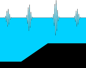
Raustøl (Reference Raustøl2014) provides experiments of wave propagation over a shoal, later summarised in Trulsen et al. (Reference Trulsen, Raustøl, Jorde and Rye2020). These experiments were carried out in a 24.6 m long and 0.5 m wide wave tank. Surface elevation measurements were made with ultrasound probes, and velocity measurements were made with an acoustic doppler velocimeter, with an array of 16 probes that was moved to four different locations such that the resolution before the shoal was 0.3 m and the resolution above the shoal was 0.1 m. The wavemaker generated a JONSWAP spectrum with peak parameter  $\gamma = 3.3$, with typical peak periods
 $T_{p} \sim 1$ s. The probability distribution of rogue waves evolving with the distance from the wavemaker was recorded, offering a benchmark for our non-homogeneous correction to the wave height probability distribution. Since our model is expressed in terms of dimensionless depth and significant steepness, we have extracted the raw data from figures 5.4 and 5.5 of Raustøl (Reference Raustøl2014), in accordance with the inversion
 $k_{p}h \approx (k_{p}a_{c}/ {Ur})^{1/3}$ of Trulsen et al. (Reference Trulsen, Raustøl, Jorde and Rye2020). In order to facilitate the processing, we have smoothed the experimental data by fitting analytic functions on the data points, as described in detail in Appendix E. The experiments feature a shoal starting at
 $x = 0$, rising up to 42 cm at
 $x$ = 1.6 m, followed by a plateau until
 $x = 3.2$ m and a decay to zero until
 $x = 4.8$ m. The initial depth ranges between 50 and 60 cm depending on the runs, as detailed in table 1 of Trulsen et al. (Reference Trulsen, Raustøl, Jorde and Rye2020) and table 5.2 of Raustøl (Reference Raustøl2014).
4.1. Results
Based on the  $\kappa _{0}$ parameterisation described in the previous section, we compute the evolution of the rogue wave probability as a function of distance for each run, assuming a pre-shoal homogeneous Rayleigh distribution (figure 5). The values of
 $\kappa _{0}$ calculated according to (3.25) amount to
 $(5.9, 4.9, 4.3, 3.6, 2.9, 2.6,2.3, 2.4, 2.3, 2.2)$ for the runs 1–2, 4–9 and 11–12, respectively. Our model that takes into account the evolution of the wave asymmetry
 $\mathfrak {S}_{0}$ over the shoal (cyan curves) due to the skewness of the surface elevation distribution (2.3) reproduces well the experimental data, over the whole shoaling episode and for all runs. Disregarding the evolution of skewness reported in Trulsen et al. (Reference Trulsen, Raustøl, Jorde and Rye2020) while keeping a vertical fixed asymmetry
 $\mathfrak {S}_{0}=1.2$ (blue curves in figure 5) degrades the agreement only marginally, although the probability rises slightly earlier, decays slightly later, and the asymmetry between the up- and down-shoaling phases is reduced. Furthermore, we point out the remarkable difference of amplification between vertically asymmetrical (solid blue, cyan) and symmetrical seas (dashed red). This happens because (3.21) leads to a maximal amplification between 75 % and 100 % for
 $\varGamma \approx 1.08\text{--} 1.10$. When we include the typical vertical asymmetry
 $\mathfrak {S}_{0}^{2} \sim 1.5$, the pre-shoal probability
 $\mathbb {P}_{\alpha }$ is transformed into
 $\mathbb {P}_{\alpha }^{2/3} \sim 10\mathbb {P}_{\alpha }$ within Regime II, seemingly becoming an alternative to Gram–Charlier models (Mori & Yasuda Reference Mori and Yasuda2002). Finally, adjusting the homogeneous pre-shoal probability to the observed values instead of considering an initial Rayleigh distribution (dotted curve) improves the agreement (runs 6–12, figures 5e–j), demonstrating the applicability of our model to arbitrary probability distributions. This agreement over the whole range of experimental conditions reported by Raustøl (Reference Raustøl2014) is remarkable, as it requires no specific parameter tweaking.
Evolution of the probability of rogue waves  $(\alpha \ge 2)$ over a shoal for Runs 1–2, 4–9, 11–12 from figure 5.8 of Raustøl (Reference Raustøl2014). Blue: model of (3.23) for a pre-shoal (
 $x < 0$) Rayleigh distribution with
 $\mathfrak {S}_{0}=1.2$. Cyan: same model, considering the evolution of skewness over the shoal. Dotted: model of (3.23) for a pre-shoal probability matched to the experimental data. Dashed: same as blue, but for symmetrical seas,
 $\mathfrak {S}_{0}=1$.

4.2. Discussion
In contrast, Tayfun (Reference Tayfun1980) (see the discussion following (36)–(38) of that paper) claims a Gaussian probability distribution for the second-order wave heights, as also discussed in Tayfun (Reference Tayfun1990) and Tayfun & Fedele (Reference Tayfun and Fedele2007). In fact, these models fall under the broad category of quasi-determinism theories (Boccotti Reference Boccotti2000), in which Longuet-Higgins (Reference Longuet-Higgins1980) and Naess (Reference Naess1985) also take part and preclude wave heights from exceeding the Rayleigh distribution, typically being lower than the latter as the bandwidth broadens. Therefore, these formulations in homogeneous conditions would not be able to describe the Raustøl (Reference Raustøl2014) and Trulsen et al. (Reference Trulsen, Raustøl, Jorde and Rye2020) experiments. Also according to these models, any departure from a Rayleigh distribution of wave heights is due to third-order nonlinearities (Tayfun & Fedele Reference Tayfun and Fedele2007; Alkhalidi & Tayfun Reference Alkhalidi and Tayfun2013). Nevertheless, it is important to remark that most of these theories were devised for deep waters, hence they fall within Regime III of our model. Moreover, following Marthinsen (Reference Marthinsen1992) and Dingemans (Reference Dingemans1997), one can tentatively elaborate alternative finite-depth second-order mathematical structures as in § 3.5. Comparing with our model, we observe a numerical equivalence in deep water, but not in transitional and shallow waters where the alternative second-order models display a sharp departure from the observations of Goda (Reference Goda1983). Unfortunately, the finite-depth model of Tayfun & Alkhalidi (Reference Tayfun and Alkhalidi2020) is not a distribution of wave heights, hence is not applicable to our discussion.
Our  $\varGamma$ model of the probability evolution over a shoal is based on the second-order correction, which is valid for
 ${Ur} \leqslant 8{\rm \pi} ^{2}/3$ (Dean & Dalrymple Reference Dean and Dalrymple1984). This limit of validity is well beyond the Ursell number
 ${Ur} \leqslant 0.22$ of the experiments considered in this work (Raustøl Reference Raustøl2014; Trulsen et al. Reference Trulsen, Raustøl, Jorde and Rye2020). We can therefore expect that the
 $\varGamma$ model will still apply to more than 10 times larger waves and/or shallower waters.
The transient drop of  $\mathbb {P}_{\alpha, \varGamma }/\mathbb {P}_{\alpha }$ to almost zero in the rising region of the shoal (
 $0 \leqslant x \le 1.6$ m) in runs 1, 2, 4 and 5, as well as its slow decay on the trailing side (
 $3.2 \le x \le 4.8$ m), could be due to higher-order nonlinear effects not captured in our model, including the evolution of the skewness and kurtosis of the surface elevation probability distribution when propagating on the shoal.
Recent developments in Zhang & Benoit (Reference Zhang and Benoit2021) described the exceedance probability of Run 3 of Trulsen et al. (Reference Trulsen, Raustøl, Jorde and Rye2020) throughout the shoaling and de-shoaling stages by means of numerical simulations. However, an analytical expression for the probability distribution was not provided, and cases with low or vanishing skewness and kurtosis like Run 12 were not addressed. Our model provides an explicit expression with no free fitting parameter. It is obtained directly from second-order correction and has been shown to be valid for all runs in Raustøl (Reference Raustøl2014). Although we were not able to analyse Run 3 (Jorde Reference Jorde2018) due to the lack of wave height probability data, we are confident that our model can reproduce it well, as it does for the very similar Runs 1, 2 and 4.
The modulational instability cannot account for the rise of the rogue wave probability due to shoaling in the considered experiments because they do not feature narrow-banded Stokes waves or lie in the optimal range  $k_{p}h > 1.36$ (Zakharov & Ostrovsky Reference Zakharov and Ostrovsky2009) in the shallower side, except for Runs 11 and 12, which showed no significant amplification. On the other hand, all runs start in the range
 $k_{p}h > 1.36$ before the shoal and showed no large deviation from the Gaussian sea, except for Run 12.
Furthermore, our model – and in particular the three regimes discussed in (3.15) and figure 1(b) – also allows us to understand the contradictory behaviours highlighted by Trulsen et al. (Reference Trulsen, Raustøl, Jorde and Rye2020) and Zhang & Benoit (Reference Zhang and Benoit2021). While the rogue wave probability is not affected by a shoal in initially deep water (Regime III), it does increase on a shoal in intermediate depth (Regime II). Interestingly, a third regime (Regime I of figure 1b) is consistent with observed surf zone statistics (Glukhovskii Reference Glukhovskii1966), i.e. rogue wave likelihood lower than in transitional waters. In addition, Barbariol et al. (Reference Barbariol, Benetazzo, Carniel and Sclavo2015) show an increase of maximum crest up to some cut-off in dimensionless depth, upon which it starts to decrease sharply the higher the ratio  $H_{1/3}/h$ becomes, thus providing support for Regime I in our model. However, numerical simulations and experiments with even shallower shoals are necessary for a conclusive assessment. Therefore, we have demonstrated that rogue wave statistics will be enhanced by non-equilibrium dynamics of rapid depth change for a dimensionless depth
 $0.5 < k_{p}h < 1.5$ but stops growing when it leaves this range. It is therefore less pronounced past the threshold
 $k_{p}h \leqslant 0.3$ until it starts to follow shallow water distributions such as in Glukhovskii (Reference Glukhovskii1966). Recently, after the submission of this work, experiments on the shoaling of irregular unidirectional waves have confirmed our prediction that the amplification of wave height statistics in Regime II will vanish in Regime I (Xu et al. Reference Xu, Liu, Li and Jia2021).
The evolution of the rogue wave probability highlighted by our model could be related to the process proposed by Li et al. (Reference Li, Zheng, Lin, Adcock and Van Den Bremer2021c) and confirmed experimentally in Li et al. (Reference Li, Draycott, Adcock and Van Den Bremer2021a), in which the generation of additional wave packets that interact with the original pre-shoal wave packet propagating over a step leads to a local peak some distance into the shallower region. Notably, Li et al. (Reference Li, Zheng, Lin, Adcock and Van Den Bremer2021c) have used a more general treatment for the surface elevation, containing both super- and sub-harmonics, as well as free and bound waves. Moreover, instead of bound super-harmonics in our model, one could investigate the effect of the nonlinear evolution of interacting free modes. For instance, similar experimental results were interpreted using a statistical matching of Korteweg–De Vries equilibrium states at the depth transition point (Majda et al. Reference Majda, Moore and Qi2019; Moore et al. Reference Moore, Bolles, Majda and Qi2020). In retrospect to the ideas in Onorato & Suret (Reference Onorato and Suret2016), these works obtained a connection between variance and skeweness with the dynamics. Therefore, subsequent investigations carrying out a comparison between the two types (free and bound) of mode evolution will be of great relevance.
5. Conclusion
This work presented a connection between statistical distributions and the fluid mechanics of the second-order perturbation in non-homogeneous conditions, providing successfully a physical explanation for the rogue wave probability increase over a depth change (Raustøl Reference Raustøl2014; Trulsen et al. Reference Trulsen, Raustøl, Jorde and Rye2020). We have shown that our model reproduces very well the experiments of Raustøl (Reference Raustøl2014) and Trulsen et al. (Reference Trulsen, Raustøl, Jorde and Rye2020) regarding the probability distribution as a function of the distance from the wavemaker. Moreover, we showed that the significant steepness and dimensionless depth affect the validity, and assessed numerically the extent of the deviation from the assumption of homogeneity. Furthermore, instead of introducing new physics (Haver & Andersen Reference Haver and Andersen2000), our model has demonstrated that an effective theory arises by challenging the homogeneity assumption. Introducing the  $H_{1/3}/\sigma$ ratio (Goda Reference Goda1983), we have established that the deep water regime produces no significant amplification of the height distribution, whereas the transitional water within
 $0.5 < k_{p}h < 1.5$ provides strong amplification, and the shallow water regime decreases this large amplification to a level smaller than the initial stage in deep water.
Our model has been restricted to reformulating normalised moments up to the variance only. The evolution of either skewness or kurtosis as a function of the distance from the wavemaker (Trulsen et al. Reference Trulsen, Raustøl, Jorde and Rye2020) will be addressed in a subsequent work. On the other hand, we have shown that it is possible to fit the data without the application of either skewness or kurtosis, as they are ‘symptoms’ of the dynamics and not the cause (Stansell Reference Stansell2004; Christou & Ewans Reference Christou and Ewans2014; Cattrell et al. Reference Cattrell, Srokosz, Moat and Marsh2018). Since our model relies on relations between steepness, slope and bandwidth that might be affected by a rapid depth change, the empirical findings in Mendes et al. (Reference Mendes, Scotti and Stansell2021) regarding vertical asymmetry have to be extended to the current setting for an exact formulation. Furthermore, the generalisation of this work to multidirectional spectra would be needed, since Ducrozet & Gouin (Reference Ducrozet and Gouin2017) suggest that such a configuration weakens the effect of a varying bathymetry. Whether rogue waves are enhanced in strong bathymetry changes throughout most oceans or regionally under suitable conditions is yet to be assessed.
Funding
S.M., M.B. and J.K. were supported by the Swiss National Science Foundation under grant 200020-175697. S.M. and A.S. were supported by the National Science Foundation under grant OCE-1558978.
Declaration of interests
The authors report no conflict of interest.
Appendix A. Spectral analysis of spatial and temporal series
Below, we discuss two aspects of the assumptions necessary to obtain a sea with Gaussian statistics, the first dealing with a steady-state treatment of the statistical moments, and the second dealing with otherwise out-of-equilibrium conditions. First, we highlight that typically, classical definitions exhibit steady-state series as stationary and homogeneous in regard to translations in time and space, respectively. Traditionally, the Khintchine (Reference Khintchine1934) theorem is often written for the time domain, but it can be generalised to the spatial domain (Ripley Reference Ripley1981; Sherman Reference Sherman2010). Indeed, the spatial Khintchine theorem has the same structure, only replacing the time lag  ${\tau }$ by a displacement vector
 ${| \pmb {\xi } | = \xi }$ (Shinozuka & Jan Reference Shinozuka and Jan1972; Deodatis & Shinozuka Reference Deodatis and Shinozuka1988; Shinozuka & Deodatis Reference Shinozuka and Deodatis1988). For mean-ergodic homogeneous processes, the autocorrelation of the sea surface elevation (here, the surface elevation
 $\zeta (x,t)$ has been denoted as
 $\zeta (x)$ to ease the notation) can be computed properly from the spatial average
 $\langle \cdot \rangle _{{x}}$ as
 \begin{equation} \left.\begin{gathered} R_{{x}} ({\xi}) := \mathbb{E}[\zeta(x)\,\zeta (x+\xi) ] = \langle \zeta(x)\,\zeta (x+\xi) \rangle_{{x}}, \\ \therefore \quad R{_{x}}(0) \equiv \langle \zeta^{2} \rangle_{{x}} = \lim_{{L} \rightarrow +\infty} \frac{1}{{L}} \int_{0}^{{L}} \zeta^{2}({x}) \,{\rm d}{x}, \end{gathered}\right\} \end{equation}
such that one can find (Boccotti Reference Boccotti2000; Goda Reference Goda2010)
 \begin{equation} R_{{x}}({\xi}) = \tfrac{1}{2} \sum_{i} a_{i}^{2} \cos ({k_{i}\xi}), \quad \therefore \quad R_{{x}}(0) =\langle \zeta^{2} \rangle_{{x}} = \tfrac{1}{2} \sum_{i} a_{i}^{2} = \mathscr{E}_{{AIRY}}. \end{equation}
Moreover, in a mean-ergodic stationary time series, the ensemble average is computed exactly from the time average  $\langle \cdot \rangle _{t}$, i.e.
 $R_{t}(\tau = 0) = \langle \zeta ^{2} \rangle _{t} = \sum _{i} a^{2}_{i}/2$. Therefore, if a sufficiently large spatiotemporal series with uniform distribution of phases is ergodic, homogeneous in space and stationary in time, then we have
 \begin{equation} \mathbb{E}[\zeta] = \langle \zeta \rangle_{{x}} = \langle \zeta \rangle_{t} = 0,\quad \mathbb{E}[\zeta^{2}]= \langle \zeta^{2} \rangle_{{x}} = \langle \zeta^{2} \rangle_{t} = \tfrac{1}{2} \sum_{i} a_{i}^{2}, \end{equation}
thus narrowing down the possible solutions into the Gaussian distribution of the surface elevation because  $\mathbb {E}[\zeta ^{2n+1}]= 0$ for all
 $n \in \mathbb {N}$ and vanishing excess kurtosis. This procedure is very common in complex physical systems, and the above property is called ergodicity (Boltzmann Reference Boltzmann1898), while proving its validity is always a challenging task (Penrose Reference Penrose1973). The exact computation of the ensemble average of the sea surface elevation at an instant of time
 $t_{0}$ is not trivial (Goda Reference Goda2010). Without ergodicity, the probability density of the surface elevation is unknown unless one assumes its expected value
 \begin{equation} \mathbb{E}\left[ \zeta \right] = \int\zeta\,{\rm d}\mu(\zeta), \end{equation}
where  $\textrm {d}\mu (\zeta )$ is a measure on the space of possible surface elevations. For an oscillatory system, it is customary to write
 $\zeta ={r}\cos (\phi )$ and introduce a joint p.d.f. on the space
 $[0,\infty )\times [0,2{\rm \pi} )$ that describes the statistical distribution of amplitudes and phases. Without loss of generality, we can always choose units in which
 $\mathbb {E}[\zeta ^{2}]=1$, and write
 \begin{equation} \mathrm{p.d.f.}=\frac{f({r},\phi)}{2{\rm \pi}}\,{r} \,{\rm e}^{-{r}^2/2}\,{\rm d}{r} \,{\rm d}\phi. \end{equation}
The distribution of Longuet-Higgins (Reference Longuet-Higgins1952) is recovered if we assume that the phases are distributed uniformly and uncorrelated from the amplitudes, that is,  $f({r},\phi )=1$ (Rice Reference Rice1945; Cramér & Leadbetter Reference Cramér and Leadbetter1967; Mori & Yasuda Reference Mori and Yasuda2002; Onorato et al. Reference Onorato, Residori, Bortolozzo, Montina and Arecchi2013). However, the uniform distribution of phases is appropriate only for narrow-banded signals (Davenport & Root Reference Davenport and Root1987; Middleton Reference Middleton1996). For more realistic sea states, Tayfun (Reference Tayfun2008) shows that the p.d.f. introduced above should be corrected to account for correlations between phase and amplitude. As a first approximation, the correction proposed by Tayfun (Reference Tayfun2008) is
 \begin{equation} f({r},\phi)=1+\frac{\mu_3}{6}{r}({r}^2-4)\cos\phi, \end{equation}
where  $\mu _3$ is the skewness. Note that within this approximation, the expected value of even-order powers of
 $\zeta$ are not modified relative to the uniform phase approximation. Odd-order powers, which are zero when
 $f=1$, are now non-zero. On the other hand, it is known that the weakly nonlinear evolution of a sea state which at
 $t=0$ has random and uniformly distributed independent phases, remains so over the nonlinear time interval
 $t \gtrsim 2{\rm \pi} /\omega _{p}$ (Choi, Lvov & Nazarenko Reference Choi, Lvov and Nazarenko2004, Reference Choi, Lvov and Nazarenko2005). Therefore, the source of correlations between phases and amplitudes cannot be attributed to the internal weakly nonlinear dynamics. However, this does not preclude that external factors (e.g. wind forcing) inducing non-equilibrium dynamics can nudge the phase distribution away from uniformity and/or impart a correlation between phases and amplitudes.
For the purpose of illustration, let us analyse the simplest effect of a uniform distribution. Through a change of variables (Papoulis Reference Papoulis2002) and the law of the unconscious statistician (Blitzstein & Hwang Reference Blitzstein and Hwang2019), we rewrite the ensemble average as
 \begin{equation} \mathbb{E}\left[ \zeta \right] = \int_{-\infty}^{+\infty} \zeta\,f(\zeta)\,{\rm d}\zeta = \int_{{0}}^{{2{\rm \pi}}} \zeta (\phi)\,f(\phi) \,{\rm d}\phi. \end{equation}
Therefore, the uniform distribution of phases leads to ergodicity:
 $$\begin{gather} \mathbb{E}\left[ \zeta \right] = \sum_{i} \frac{a_{i}}{2{\rm \pi}} \int_{0}^{2{\rm \pi}} \cos \phi \,{\rm d}\phi = \langle \zeta ({x}) \rangle = \lim_{{L} \rightarrow +\infty} \sum_{i} \frac{a_{i}}{{L}} \int_{0}^{{L}} \cos{({k_{i}x})} \,{\rm d}{x} = 0, \end{gather}$$
 $$\begin{gather}\mathbb{E}[ \zeta^{2} ] = \sum_{i} \frac{a_{i}^{2}}{2{\rm \pi}} \int_{0}^{2{\rm \pi}} \cos^{2} \phi \,{\rm d}\phi = \langle \zeta^{2} ({x}) \rangle = \lim_{{L} \rightarrow +\infty} \sum_{i} \frac{a^2_{i}}{{L}} \int_{0}^{{L}} \cos^2{({k_{i}x})}\, {\rm d}{x} = \sum_{i} \frac{a_{i}^{2}}{2}. \end{gather}$$
If we assume that correlations develop between the phases, then a weak departure from ergodicity will be observed. Below we show that due to the ergodicity assumption, the accuracy of Gaussian statistics will deteriorate, the narrower the superposition distribution. For the sake of measuring appreciable deviations and without loss of generality, we use a Boltzmann-like distribution, such that the ensemble average of the sea surface reads
 \begin{equation} \mathbb{E}^{(B)}\left[ \zeta \right] = \sum_{i} \left[ \frac{a_{i}}{\rm \pi}\int_{0}^{+\infty} \frac{\cos \phi}{{\rm e}^{\phi/{\rm \pi}}}\,{\rm d}\phi \right] = \sum_{i} \frac{a_{i}}{(1+{\rm \pi}^{2})} \sim 0.2\sqrt{m_{0}}, \end{equation}
which is relatively small compared to the second moment of the surface elevation. For a tentative Gaussian-shaped superposition, however, one finds
 \begin{equation} \mathbb{E}^{(G)}\left[ \zeta \right] \approx \sum_{i} a_{i} \left[ \frac{3}{5}\int_{0}^{+\infty} \cos \phi \,{\rm e}^{-(\phi-1)^{2}} \,{\rm d}\phi \right] = \sum_{i} \frac{3a_{i}}{8} \sim 0.{8}\sqrt{m_{0}}, \end{equation}
while for the square of the surface elevation we obtain
 \begin{align} \mathbb{E}^{(B)}[ \zeta^{2} ] &\approx \sum_{i} \frac{a_{i}^{2}}{\rm \pi} \int_{0}^{+\infty} {\rm e}^{-\phi/{\rm \pi}} \cos^{2} \phi \,{\rm d}\phi + \sum_{i\neq j} \frac{a_{i} a_{j}}{\rm \pi} \int_{0}^{+\infty} {\rm e}^{-\phi/{\rm \pi}} \cos \phi \,{\rm d}\phi \nonumber\\ &\approx \left( \frac{1+2{\rm \pi}^{2}}{1+4{\rm \pi}^{2}} \right) \sum_{i} a_{i}^{2} + \sum_{i\neq j} \frac{a_{i} a_{j}}{1+{\rm \pi}^{2}}\sim \left( \frac{4+14{\rm \pi}^{2}+4{\rm \pi}^{4}}{1+5{\rm \pi}^{2}+4{\rm \pi}^{4}} \right) m_{0} \sim 1.2 m_{0}. \end{align}
Lacking a closed form, the Gaussian-like distribution of phases reads, instead,
 \begin{equation} \mathbb{E}^{(G)}[ \zeta^{2} ] \approx \sum_{i} \frac{5a_{i}^{2}}{13} + \sum_{i\neq j} \frac{3a_{i} a_{j}}{8} \sim 1.53 m_{0}. \end{equation}
Comparing the deviations from the uniform superposition in (A10)–(A12) gives
 \begin{equation} \delta \mathbb{E}^{(B)}_{1,2} = \frac{\sqrt{ \mathbb{E}^{(B)}[\zeta^{2}] - \mathbb{E}^{(U)}[\zeta^{2}] }}{\mathbb{E}^{(B)}[\zeta] - \mathbb{E}^{(U)}[\zeta]} = \frac{\sqrt{1.2 m_{0} - m_{0}}}{0.2 \sqrt{m_{0}} - 0} \approx 2.3, \end{equation}
whereas for the Gaussian one we have
 \begin{equation} \delta \mathbb{E}^{(G)}_{1,2} = \frac{\sqrt{ \mathbb{E}^{(G)}[\zeta^{2}] - \mathbb{E}^{(U)}[\zeta^{2}] }}{\mathbb{E}^{(G)}[\zeta] - \mathbb{E}^{(U)}[\zeta]} = \frac{\sqrt{1.53 m_{0} - m_{0}}}{0.{8} \sqrt{m_{0}} - 0} \approx 0.9, \end{equation}
implying a decreasing gap between moments when the superposition distribution is narrower. In these examples, we see that even the linear evolution of a sea state that at some point in time has a non-uniform distribution of phases breaks ergodicity. We remark that the break in ergodicity and being Gaussian are not necessarily simultaneous, as in the above case.
Appendix B. Energetic formulae derivation
Given (3.6) and taking the limit of very large number of amplitude components towards an asymptotic leading order, the energy computation is reduced to the coefficients  $(\varOmega _{m},\tilde {\varOmega }_{m})$. Then, having
 $u_{i} = \partial {\varPhi }/\partial x_{i}$ and using the notation
 $I={u^{2}_{1}} + {u^{2}_{3}}$, one obtains
 \begin{align} I &= \left[ \frac{\partial}{\partial x} \left\{ \sum_{j} f_{j} \cosh{(j \varphi)} \sin{(j \phi)} \right\} \right]^{2} + \left[ \frac{\partial}{\partial z} \left\{ \sum_{j} f_{j} \cosh{(j \varphi)} \sin{(j \phi)} \right\} \right]^{2} \nonumber\\ &= \left[ \sum_{j} jk \times f_{j} \cosh{(j \varphi)} \cos{(j\phi)} \right]^{2} + \left[ \sum_{j} jk \times f_{j} \sinh{(j \varphi)} \sin{(j\phi)} \right]^{2} \nonumber\\ &= \left[ \sum_{m} \varOmega_{m} \cosh{(m \varphi)} \cos{(m\phi)} \right] \left[ \sum_{n} \varOmega_{n} \cosh{(n \varphi)} \cos{(n\phi)} \right] \nonumber\\ &\quad +\left[ \sum_{m} \varOmega_{m} \sinh{(m \varphi)} \sin{(m\phi)} \right] \left[ \sum_{n} \varOmega_{n} \sinh{(n \varphi)} \sin{(n\phi)} \right], \end{align}
where we defined  $\varOmega _{m} = mk f_{m}$ and estimated the effect of
 $|\partial h/\partial x|$ to not be of leading order for this sum (see §§ 3 and 4.2). By means of the notation
 \begin{equation} \mathfrak{Cos}_{mn} (\varphi, \phi ) := \cosh{(m\varphi)} \times \cos{(n \phi)};\quad \mathfrak{Sin}_{mn} (\varphi, \phi ) := \sinh{(m\varphi)} \times \sin{(n \phi)}, \end{equation}
the algebra yields
 \begin{align} I &= \sum_{m=n} \varOmega_{m}^{2}\,\mathfrak{Cos}^{2}_{mm} (\varphi,\phi ) + \sum_{m\neq n} \varOmega_{m} \varOmega_{n}\,\mathfrak{Cos}_{mm} (\varphi,\phi )\, \mathfrak{Cos}_{nn} (\varphi,\phi) \nonumber\\ &\quad +\sum_{m=n} \varOmega_{m}^{2}\,\mathfrak{Sin}^{2}_{mm} (\varphi,\phi) + \sum_{m\neq n} \varOmega_{m} \varOmega_{n}\,\mathfrak{Sin}_{mm} (\varphi,\phi)\, \mathfrak{Sin}_{nn} (\varphi,\phi ) \nonumber\\ &:= \sum_{m} \varOmega_{m}^{2} I_{mm} + \sum_{m\neq n} \varOmega_{m} \varOmega_{n} I_{mn}. \end{align}
However, one can further expand the trigonometric clusters in (B2) as follows:
 \begin{align} 4I_{mn} &= 4\,\mathfrak{Cos}_{mm} (\varphi,\phi)\,\mathfrak{Cos}_{nn} (\varphi, \phi ) + 4\,\mathfrak{Sin}_{mm} (\varphi,\phi )\,\mathfrak{Sin}_{nn} (\varphi, \phi ) \nonumber\\ &= \left[\cos{(m \phi)} \cos{(n \phi)} + \sin{(m \phi)} \sin{(n \phi)}\right] \times 2\cosh{\left[ (m+n) \varphi \right]} \nonumber\\ &\quad + \left[\cos{(m \phi)} \cos{(n \phi)} - \sin{(m \phi)} \sin{(n \phi)}\right] \times 2\cosh{\left[ (m-n) \varphi \right]} \nonumber\\ &= 2 \cosh{\left[ (m+n) \varphi\right]} \cos{\left[ (m-n) \phi\right]} + 2 \cosh{\left[ (m-n) \varphi\right]} \cos{\left[ (m+n) \phi\right]}. \end{align}
As an immediate corollary, we find  $2I_{mm} = \cosh {(2m \varphi )} + \cos {(2m \phi )}$. Using the algebra from (B4) and periodic integration, following the expression for the energy in (2.4) and subtracting the potential energy
 $\rho g h_{0}^{2}/2$ due to the water column, we find in the limit
 $i \rightarrow \infty$ the leading-order energy density
 \begin{equation} \mathscr{E} \approx \sum_{m} \frac{\tilde{\varOmega}_{m}^{2}}{4} + \sum_{m} \frac{\varOmega_{m}^{2}}{4g} \int_{{-}h}^{0} \cosh{\left(2m\varphi \right)} \,{\rm d} z \approx \frac{1}{4} \sum_{m} \left[ \tilde{\varOmega}_{m}^{2} + \varOmega_{m}^{2}\, \frac{ \sinh{(2mkh)}}{2mgk} \right]. \end{equation}
As we assumed a small effect of  $\partial h/\partial x$ in the previous integral, the bathymetry will appear in
 $\varphi = k (z+h)$ as well as in
 $\varOmega _{m}$ and
 $\tilde {\varOmega }_{m}$. Likewise, using the definition of (3.6), and taking into account the discussion in (3.2) and (3.3), we compute the time average of the squared sea surface elevation at a fixed point
 $x_{i} \in \mathbb {R}$:
 \begin{equation} \langle \zeta^{2} \rangle_{{t}} = \lim_{{T} \rightarrow +\infty} \frac{1}{{T}} \int_{0}^{{T}} \left[ \sum_{m} \tilde{\varOmega}_{m} \cos{(m\phi)} \right] \left[\sum_{n} \tilde{\varOmega}_{n} \cos{(n\phi)} \right] {\rm d}{t} = \sum_{m} \frac{\tilde{\varOmega}_{m}^{2}}{2}, \end{equation}
where the function  $\tilde {\varOmega }_{m} = \tilde {\varOmega }_{m}(x)$ is also a function of
 $x$ due to its dependence on significant steepness
 $\varepsilon = \varepsilon (x)$ and dimensionless depth
 $k_{p}h = (k_{p}h)(x)$. To compare the generalised model with the specific case of Airy's solution, we set
 $m = 1$. In this case,
 $\tilde {\varOmega }_{1} = a$ while
 $\varOmega _{1} = ag k/\omega \cosh {kh}$ (Dingemans Reference Dingemans1997), the dispersion relation is expressed as
 $\omega ^{2} = gk \tanh {kh}$, so that the spatial energy density is
 \begin{align} \mathscr{E}_{1} &= \frac{1}{4} \left[ a^{2} + \left( \frac{agk}{\omega \cosh{kh}} \right)^{2} \frac{ \sinh{(2kh)}}{2gk} \right] \nonumber\\ &= \frac{1}{4} \left[ a^{2} + \left( \frac{a^{2}g^{2}k^{2}}{gk \tanh{kh} \times \cosh^{2}{kh}} \right) \frac{ 2 \sinh{kh} \cosh{kh}}{2gk} \right] = \frac{a^{2}}{2}, \end{align}
thus recovering the spatial energy density in (2.6). For the second order, we have
 \begin{equation} \varOmega_{1} = \frac{a\omega}{ \sinh{kh}}, \quad \varOmega_{2} = \frac{3ka^{2} \omega}{ 4 \sinh^{4}{kh}},\quad \tilde{\varOmega}_{1} = a,\quad \tilde{\varOmega}_{2} = \frac{ka^{2}\cosh{kh} }{ 4 \sinh^{3}{kh}} \left[ 2+ \cosh{(2kh)} \right]. \end{equation}
Upon the steepness being expressed as  $ka { = (2{\rm \pi} /\lambda ) \times (H/2)} = {\rm \pi}\varepsilon$, the spatial energy density is computed and leads to (3.10a,b)–(3.11a,b):
 \begin{align} \mathscr{E}_{2} &= \frac{a^{2}}{2} + \frac{1}{4} \left\{ \frac{k^{2}a^{4}}{16} \left[ \frac{\cosh{kh} }{\sinh^{3}{kh}} \left( 2+ \cosh{(2kh)} \right) \right]^{2} + \left( \frac{3ka^{2} \omega}{ 4 \sinh^{4}{kh}} \right)^{2} \frac{ \sinh{(4kh)}}{4gk} \right\} \nonumber\\ &= \frac{a^{2}}{4} \left\{ 2 + \left( \frac{{\rm \pi}\varepsilon}{4} \right)^{2} \left[ \frac{\cosh{kh} }{\sinh^{3}{kh}} \left( 2+ \cosh{(2kh)} \right) \right]^{2} + \left( \frac{{\rm \pi}\varepsilon}{4} \right)^{2} \left[ \frac{9 \cosh{(2kh)}}{\sinh^{6}{kh}}\right] \right\}. \end{align}
Appendix C. Amplification universality
Here we will prove the validity of the two relations in (3.23). The result in (3.23) assures us of the invariance of the ratio of logarithms in (3.21) and the amplification (ratio of probabilities) in (3.22), regardless of the equilibrium exceedance probability prior to the shoal. Let us set up a general expression to accommodate both super-Rayleigh ( $+$) and sub-Rayleigh (
 $-$) distributions, e.g. those that assign higher or lower probabilities than prescribed by Longuet-Higgins (Reference Longuet-Higgins1952) at either the bulk or tail of the distribution. We attach a factor
 $g_{\mu \alpha }^{\pm }$ to the Rayleigh distribution, denoting a Gram–Charlier (GC) series (Longuet-Higgins Reference Longuet-Higgins1963; Mori & Yasuda Reference Mori and Yasuda2002). Equation (3.23) holds if one can prove that the variance is corrected by a negligible term, denoted by
 $\mathfrak {L}_{\mu }$:
 \begin{equation} \mathbb{P}^{{\pm}}_{\alpha,\mu} = g_{\mu \alpha}^{{\pm}} \times \mathcal{R}_{\alpha}, \quad \therefore \quad \mathbb{P}^{{\pm}}_{\alpha,\mu} (\varGamma) = \left( \mathbb{P}^{{\pm}}_{\alpha,\mu} \right)^{{1}/{\varGamma \pm \mathfrak{L}_{\mu}}} = \left( g_{\mu \alpha}^{{\pm}} \,{\rm e}^{{-}2\alpha^{2}} \right)^{{1}/{\varGamma \pm \mathfrak{L}_{\mu}}}. \end{equation}
We will show that this term satisfies  $\mathfrak {L}_{\mu }\ll \varGamma$. Without loss of generality, the dual GC-
 $\zeta$ distribution with
 $|\mu _{3}|=|\mu _{4}|=1/2$ reads (Mori & Yasuda Reference Mori and Yasuda2002)
 \begin{equation} f^{{\pm}}_{\mu}(\zeta) \equiv f_{\zeta}(m_{0}) \times g_{\mu \zeta}^{{\pm}} = \frac{{\rm e}^{-\zeta^{2}/2m_{0}} }{\sqrt{2{\rm \pi} m_{0}}} \left[ 1 \pm \frac{1}{12} ( \zeta^{3} - 3 \zeta ) \pm \frac{1}{48} ( \zeta^{4} -6 \zeta^{2} + 3 ) \right]. \end{equation}
Clearly, the term  $g_{\mu \alpha }^{\pm }$ is a by-product of the surface elevation counterpart
 $g_{\mu \zeta }^{\pm }$. Hence the following model captures the features of the two non-Gaussian distributions while being properly normalised:
 \begin{equation} \frac{16}{16 \mp (\varGamma-1)^2} \int_{-\infty}^{+\infty} f_{\zeta}(m_{0}\varGamma) \times g_{\mu \zeta}^{{\pm}} \,{\rm d}\zeta = \int_{-\infty}^{+\infty} f^{{\pm}}_{\mu}(\zeta, \varGamma)\,{\rm d}\zeta = 1. \end{equation}
The first normalised moments read (see figure 6)
 \begin{equation} \mu_{1}^{{\pm}} = \int_{-\infty}^{+\infty} \frac{{16} g_{\mu \zeta}^{{\pm}}\,f_{\zeta}(\varGamma)\,\zeta}{{16 \mp (\varGamma-1)^2}}\,{\rm d}\zeta ={\pm} \frac{4\varGamma (\varGamma -1 )}{\left[ 16 \mp (\varGamma-1)^2 \right]}, \end{equation}
while the sub-Rayleigh second normalised moment is expressed as
 \begin{align} \mu_{2}^{-} = \int_{-\infty}^{+\infty} \frac{{16} g_{\mu \zeta}^{-}\,f_{\zeta}(\varGamma)\,(\zeta - \mu_{1}^{-})^{2}}{{16 + (\varGamma-1)^2}}\,{\rm d}\zeta = \varGamma \left[ 1 + \frac{4\varGamma^{4} - 28\varGamma^{3} - 20\varGamma^{2} + 44\varGamma}{\left( 15 + 2\varGamma - \varGamma^{2} \right)^{2}} \right], \end{align}
and the super-Rayleigh (see figure 6) as
 \begin{align} \mu_{2}^{+} = \int_{-\infty}^{+\infty} \frac{{16} g_{\mu \zeta}^{+}\,f_{\zeta}(\varGamma)\, (\zeta - \mu_{1}^{+})^{2}}{{16 - (\varGamma-1)^2}}\,{\rm d}\zeta = \varGamma \left[ 1 + \frac{4\varGamma^{4} - 28\varGamma^{3} + 108 \varGamma^{2} - 84\varGamma}{\left( 17 - 2\varGamma + \varGamma^{2} \right)^{2}} \right]. \end{align}
Comparing the variances with the exponent in (C1), we find  $\mu _{2}^{\pm }= \varGamma (1 {\pm \mathfrak {L}_{\mu }}/\varGamma )$, and the corrections
 ${\mathfrak {L}_{\mu }}$ can be available readily by isolating the quotients inside the brackets of the right-hand sides of the above equations. These coefficients can be further approximated (recalling that
 $|\varGamma - 1| \ll 1$) as
 \begin{equation} | \mu_{1}^{{\pm}} | \approx \frac{(\varGamma -1 )}{4}, \quad \mu_{2}^{{\pm}} \approx \varGamma \pm \frac{( \varGamma - 1 )}{3}. \end{equation}
Then we showed a weak proof of the first part of (3.23) by demonstrating that a change  $g_{\mu \alpha }^{\pm }$ in the pre-shoal Rayleigh probability will always be met by a change
 $\pm \mathfrak {L}_{\mu }$ in the variance, typically obeying
 $\mathfrak {L}_{\mu } / \varGamma \ll 1$ (see figure 6b).
 $\varGamma$-GC model: (a) ensemble average of the surface elevation; (b) its variance.

C.1. Generalised proof
In this subsection, we use the  $\varGamma$-GC model to obtain exact closed-form wave height distributions, following the steps for the integration of the envelope in a two-dimensional random walk of Mori & Yasuda (Reference Mori and Yasuda2002). Thus we integrate the joint distribution of both surface elevation
 $\zeta$ and its Hilbert transform
 $\tilde {\zeta }$ over the uniform distribution of phases, obtaining the marginal density of the surface envelope:
 \begin{equation} f^{{\pm}}_{\mu, R}(\varGamma)= \int_{0}^{2{\rm \pi}} g_{\mu \zeta}^{{\pm}}\,f_{\zeta}^{{\pm}}(\varGamma) \times g_{\mu \tilde{\zeta}}^{{\pm}}\,f_{\tilde{\zeta}}^{{\pm}}(\varGamma)\,R \,{\rm d}\phi, \end{equation}
where  $\sqrt {\zeta ^{2}+\tilde {\zeta }^{2}}= R$ is the envelope with
 $\zeta = R \cos \phi$ and
 $\tilde {\zeta } = R \sin \phi$. Performing this integration, changing variables to wave heights and later normalising by
 $H_{1/3}=4m_{0}=4$ and integrating again as in (2.2), we find (see figures 7a,b)
 \begin{align} \mathbb{P}_{\alpha,\mu}^{{\pm}}(\varGamma) = \frac{{\rm e}^{{-}2\alpha^{2}/\varGamma} }{3 } & \left[1 + \frac{2\alpha^{8} + 4\alpha^{6} (\varGamma - 4) + 6\alpha^{4} (\varGamma^{2} -4\varGamma + 6 \pm 32) }{[16 \mp (\varGamma-1)^2]^{2}} \right.\nonumber\\ & \left. + \frac{ 3\alpha^{2} (\varGamma - 2) (\varGamma^{2} - 2\varGamma +2 \pm 32)}{[16 \mp (\varGamma-1)^2]^{2}} \right]. \end{align}
Then, in analogy with (3.21), we are able to assess whether the proposition in (C1) holds by verifying the ratio
 \begin{equation} \frac{ \ln \left[
\mathbb{P}_{\alpha,\mu}^{{\pm}}\right]}{ (
\varGamma \pm {\mathfrak{L}_{\mu}} )\ln \left[
\mathbb{P}_{\alpha,\mu}^{{\pm}}(\varGamma) \right] } =
1, \quad \therefore \quad \frac{ \ln \left[
\mathbb{P}_{\alpha, \mu}^{{\pm}}\right] }{
\varGamma \ln \left[ \mathbb{P}_{\alpha,
\mu}^{{\pm}}(\varGamma) \right] } = 1 \pm
\frac{{\mathfrak{L}_{\mu}}}{\varGamma} \approx 1.
\end{equation}
Accordingly, figures 7(c,d) display the magnitude of the correction  $1 \pm \mathfrak {L}_{\mu }/\varGamma$ in the variance. When
 $\varGamma \approx 1.15$, we see that super-Rayleigh distributions have a maximal 4 % increase in the variance
 $\varGamma$, whereas sub-Rayleigh distributions exhibit the opposite but of smaller magnitude, confirming the estimates in the weak proof. As the validity of (C1) has been demonstrated, one can prove the universality of the amplification regardless of the distribution, i.e. extend (3.22) to an arbitrary distribution. Having in mind the order of magnitude of
 ${\mathfrak {L}_{\mu }}/\varGamma$, we can rewrite (C1) (defining
 $| {\ln g_{\mu \alpha }^{\pm }}|= \ln g_{\mu \alpha }$) as
 \begin{equation} \mathbb{P}^{{\pm}}_{\alpha,\mu} (\varGamma) = (\exp({-2\alpha^{2} \pm \ln g_{\mu \alpha}}))^{{1}/{\varGamma \pm {\mathfrak{L}_{\mu}}}} \approx \exp \left[ - \frac{2\alpha^{2}}{\varGamma}\left( 1 \mp \frac{\ln g_{\mu \alpha}}{2\alpha^{2}} \right) \left( 1 \mp \frac{{\mathfrak{L}_{\mu}}}{\varGamma} \right) \right]. \end{equation}
Furthermore, the relative probability becomes
 \begin{align}
\frac{\mathbb{P}^{{\pm}}_{\alpha, \mu}
(\varGamma)}{\mathbb{P}^{{\pm}}_{\alpha, \mu}} &= \exp
\left[({-}2\alpha^{2} \pm \ln g_{\mu \alpha})
\left(\frac{1}{\varGamma \pm {\mathfrak{L}_{\mu}}}-1
\right) \right] \nonumber\\ &= \exp \left[
2\alpha^{2} \left( 1 \mp \frac{\ln g_{\mu
\alpha}}{2\alpha^{2}} \right) \left( 1 - \frac{1}{\varGamma
\pm {\mathfrak{L}_{\mu}}} \right) \right] \nonumber\\ &= \exp \left[ 2\alpha^{2} \left( 1 -
\frac{1}{\varGamma} \right) \left( 1 \mp \frac{\ln g_{\mu
\alpha}}{2\alpha^{2}} \right) \left( 1 \pm
\frac{{\mathfrak{L}_{\mu}}}{\varGamma^{2} \left( 1 -
\frac{1}{\varGamma} \right)} \right) \right] \nonumber\\ &= \mathrm{exp} \left[ 2\alpha^{2} \left( 1 -
\frac{1}{\varGamma} \right) \left( 1 \mp \frac{\ln g_{\mu
\alpha}}{2\alpha^{2}} \right) \left( 1 \pm
\frac{{\mathfrak{L}_{\mu}}}{\varGamma \left( \varGamma - 1
\right)} \right) \right] \nonumber\\ &\equiv
\exp \left[ 2\alpha^{2} \left( 1 - \frac{1}{\varGamma}
\right) (1 \mp \delta_{\mu \alpha})(1 \pm \delta_{\mu
\varGamma}) \right]. \end{align}
As  $|\varGamma - 1| \ll 1$, it is straightforward to see that
 $\delta _{\mu \varGamma }=\mathfrak {L}_{\mu }/\varGamma ( \varGamma - 1 ) \sim 10{\mathfrak {L}_{\mu }} \sim {\delta _{\mu \alpha }} = (\ln g_{\mu \alpha })/2\alpha ^{2}$, plotted for comparison in figure 8. Hence we conclude that for the probability amplification, the second correction term
 $\delta _{\mu \varGamma }$ counters
 $\delta _{\mu \alpha }$. Thus we have proved the first-order amplification universality with
 $\mu _{3}\sim \mu _{4} < 1$:
 \begin{align} \frac{\mathbb{P}^{{\pm}}_{\alpha,\mu}(\varGamma)}{\mathbb{P}^{{\pm}}_{\alpha, \mu}} &= \exp\left({2\alpha^{2} \left(1 - \frac{1}{\varGamma} \right) \pm {O}(\varGamma - 1)}\right) \nonumber\\ &\approx \exp\left({ 2\alpha^{2} \left( 1 - \frac{1}{\varGamma} \right)}\right) \equiv \frac{\mathcal{R}_{\alpha}(\varGamma)}{\mathcal{R}_{\alpha}},\quad \forall\ g_{\mu \alpha}^{{\pm}} \in \mathbb{R}_{+}. \end{align}
Rogue waves in (3.24) have  $2\alpha ^{2} [ 1 - (\mathfrak {S}_{0}^{2}\varGamma )^{-1} ] \leqslant 3$, resulting in maximal correction
 $\textrm {e}^{\mathcal {O}(\varGamma - 1)} \approx \,\textrm {e}^{3 \times 0.03} < 1.1$, suggesting an upper bound of 8–9 % variation from the universal amplification. On the other hand, figure 8 shows
 $(1 \mp \delta _{\mu \alpha })(1 \pm \delta _{\mu \varGamma }) \approx 1.14$ for ordinary waves (
 $\alpha \leqslant 1$) instead of
 $(1 \mp \delta _{\mu \alpha })(1 \pm \delta _{\mu \varGamma }) \leqslant 1.04$ for rogue waves, such that the main term of (3.24) becomes
 $2\alpha ^{2} [ 1 - (\mathfrak {S}_{0}^{2}\varGamma )^{-1} ] \leqslant 1$, and the first-order correction reads
 $\textrm {e}^{\mathcal {O}(\varGamma - 1)} \approx \textrm {e}^{0.6 \times 0.15} < 1.1$. Hence the bound is upheld by any normalised wave height.


Comparison between first-order corrections to the amplification of the  $\varGamma$-GC exceedance probability for positive skewness and kurtosis as in (C12).

Appendix D. Parameterisation generality and compact formulation
Under adequate conditions of  ${Ur \leqslant 8{\rm \pi} ^{2}/3}$ (Dean & Dalrymple Reference Dean and Dalrymple1984) and for shoals in Regime II, (3.26) can be rewritten in a more compact form. First, however, let us demonstrate that (3.26) holds regardless of which reference steepness is chosen to compute
 $\kappa _{0}$. For relatively higher or lower reference steepness
 $\varepsilon _{\pm } = \langle \varepsilon \rangle \pm \delta \varepsilon$, we find
 \begin{equation} \kappa_{0}^{{\pm}} = \frac{ \ln{ \left[ { \textrm{max}} \, \mathfrak{S}_{0} \right]} }{ \ln{\left[ \mathrm{max} \, \varGamma \left( \langle \varepsilon \rangle \pm \delta \varepsilon, k_{p}h, \mathfrak{S}_{0} \right) \right] } } \approx \kappa_{0} \mp \delta \kappa_{0}, \end{equation}
in turn affecting the probability amplification only marginally:
 \begin{equation} {\left( \frac{ \ln \mathbb{P}_{\alpha} }{\ln \mathbb{P}_{\alpha, \varGamma} } \right)_{{\pm}} = \left[\varGamma_{0} \pm \delta \varGamma_{0} \right]^{2\kappa_{0}\mp 2 \delta \kappa_{0}} \times \varGamma \left(\varepsilon (x), k_{p}h (x), \mathfrak{S}_{0} \right) \approx \frac{ \ln \mathbb{P}_{\alpha} }{\ln \mathbb{P}_{\alpha, \varGamma}}.} \end{equation}
This relation holds because the typical difference between the  $\varGamma$ correction atop the shoal and the average moving during the shoal does not exceed
 $\delta \varGamma _{0}/ \varGamma _{0} \leqslant 2\,\%$. We corroborate this by comparing the equivalent of figure 5(a) for a 0.5 % higher
 $\varGamma$ correction than its reference
 $\varGamma _{0} = 1.031$ in figure 9(a). Considering that Run 1 had maximal correction
 $\varGamma \approx 1.041$, the choice for the reference
 $\kappa _{0}$ does not affect the validity of (3.26). To obtain a compact formulation of (3.26), we notice that at a fixed point in space, i.e. at a distance
 $x=x_{i}$ from the wavemaker, the asymmetry
 $\mathfrak {S}_{0}$ does not depend on how we plot
 $\varGamma$. Therefore, we can approximate
 \begin{equation} \mathfrak{S}_{0} (x=x_{i}) = \left[ \varGamma \left(\varepsilon (x_{i}), k_{p}h (x_{i}), \mathfrak{S}_{0} \right) \right]^{\kappa_{x}} \approx \left[\varGamma \left( \langle \varepsilon \rangle, k_{p}h, \mathfrak{S}_{0} \right) \right]^{\kappa_{0}},\quad \forall\ x_{i} \in \mathbb{R}. \end{equation}
As the two versions of the  $\varGamma$ correction differ, as shown in figure 9(b), one concludes that
 $\kappa (k_{p}h) \equiv \kappa _{0} \neq \kappa _{x}$. Thus we obtain
 \begin{equation} \ln \mathfrak{S}_{0} \approx \langle \kappa_{x} \rangle \ln \langle \varGamma (x) \rangle \approx \kappa_{0} \ln \left\langle \varGamma \left( \langle \varepsilon \rangle, k_{p}h, \mathfrak{S}_{0} \right)\right\rangle, \end{equation}
whose Regime II restriction is translated numerically to  $\varGamma \geqslant 1 + \mathcal {O}(g^{-2})$, leading to
 $\langle \kappa _{x} \rangle \approx {0.64} \kappa _{kh}$, as shown in figure 9(b). Therefore, we can estimate conservatively throughout the entire trajectory:
 \begin{equation} \left[ \varGamma \left( \langle \varepsilon \rangle, k_{p}h, \mathfrak{S}_{0} \right) \right]^{2\kappa_{0}} \approx \left[ \varGamma \left(\varepsilon (x), k_{p}h (x), \mathfrak{S}_{0} \right) \right]^{1.2\kappa_{0}}. \end{equation}
Thus the ratio of the probabilities is better estimated and greatly simplified as
 \begin{equation} \frac{\ln \mathbb{P}_{\alpha} }{\ln \mathbb{P}_{\alpha, \varGamma}} \approx \left[\varGamma \left(\varepsilon (x), k_{p}h (x), \mathfrak{S}_{0}\right)\right]^{1+1.2\kappa_{0}}. \end{equation}
(a) Equivalent of figure 5(a) for a higher reference  $\varGamma$ correction due to steepness
 $\varepsilon _{+} \approx 1.16 \langle \varepsilon \rangle$ (dashed) and its original description according to (3.26) (solid). Notice that this 16 % increase in the reference steepness decreases the blue curve model by 4 % and the cyan one by 2 %. (b) Plot of
 $\varGamma$ correction for Runs 1–4 of Raustøl (Reference Raustøl2014) as a function of dimensionless depth (dashed) and distance from the wavemaker (solid) with variables
 $(\varepsilon, kh)$ modelled by Appendix E, whereas the minimum threshold applicable (
 $\varGamma \geqslant 1.01$) representative of Regime II is depicted by the thin horizontal line. The averages over these ranges read approximately
 $\langle \varGamma (x) \rangle = 1.03{6}$ and
 $\langle \varGamma (k_{p}h) \rangle = 1.02{3}$.

Appendix E. Analytical description of steepness and depth
In order to smooth as well as to facilitate the handling of the experimental data on wave steepness and dimensionless depth, we fitted them against analytic functions, as follows:
 \begin{align} \varepsilon &= \varepsilon_{1} + \varepsilon_{2}\exp(-(x-2.4)^{4}) + \varepsilon_{3} \exp({-(2+\delta_{31})[x-1.4+\delta_{32}]^{2}}) \nonumber\\ &\quad +\varepsilon_{4} \exp({-(1+\delta_{41})[x-4.9+\delta_{42}]^{2}}), \end{align}
while the modelling for the depth is computed as
 \begin{align} k_{p}h &= D_{1} + D_{2} \exp(-0.25(x-2.4)^{4}) + D_{3} \exp({-2[x+\delta_{62}-0.7]^{2}}) \nonumber\\ &\quad + D_{4} \exp({-2[x+\delta_{82}-4.2]^{2}}). \end{align}
The values of these coefficients for ten runs of Raustøl (Reference Raustøl2014) and Trulsen et al. (Reference Trulsen, Raustøl, Jorde and Rye2020) are given in table 1. As displayed in figure 10, these fits provide an accurate description of the actual data. Re-scaled by  ${\rm \pi} /4$, the first steepness coefficient
 $\varepsilon _{1}$ is equal to the pre-shoal steepness in table 1 of Trulsen et al. (Reference Trulsen, Raustøl, Jorde and Rye2020), while
 $\varepsilon _{1}+\varepsilon _{2}$ is the shallower steepness of the shoal. Likewise, the coefficient
 $D_{1}$, which was extracted from Raustøl (Reference Raustøl2014) through the formula
 $k_{p}h \approx ({\rm \pi} \varepsilon /4 {Ur})^{1/3}$ (see Trulsen et al. Reference Trulsen, Raustøl, Jorde and Rye2020), equals approximately the largest values of the dimensionless depth, while
 $D_{1}+D_{2}$ recovers the smallest values. Note, however, that Trulsen et al. (Reference Trulsen, Raustøl, Jorde and Rye2020) display the averages of each side, while we model every value according to the 16 probes of figure 2 in Trulsen et al. (Reference Trulsen, Raustøl, Jorde and Rye2020).

Modelling of the significant steepness in Raustøl (Reference Raustøl2014) experiments according to (E1), corrected to the term  $\varepsilon = {H_{1/3}/{\bar {\lambda }}}=({4}/{{\rm \pi} }) k_{p}a_{c}$. Dots represent data extracted from figure 5.4 of Raustøl (Reference Raustøl2014). Vertical dashed lines depict the rising shoal end (
 $x=1.6$) and beginning of the descending shoal (
 $x=3.2$).


 Open access

