Between 1930 and 1940, the rural farm electrification rate in the United States increased by 230 percent. Access to electricity has long been considered a major contributor to the economic welfare of populations. Households with electricity use a broader range of consumer goods and have better access to information, while for farms and firms it enhances productivity in a variety of ways. These anticipated benefits have led the World Bank to provide extensive loans and grants to aid less developed countries in bringing electricity to the 1.3 billion people in the world that live without it (IEA 2011).Footnote 1 A number of recent studies have examined the effects on economic activity of new dams and other large infrastructure projects, which include increased access to electricity as a significant benefit (Duflo and Pande Reference Duflo and Pande2007; Kitchens Reference Kitchens2014; Kline and Moretti Reference Kline and Moretti2014; Lipscomb, Mobarak, and Bahram Reference Lipscomb, Mobarak and Barham2012; Severnini Reference Severnini2012). Yet, these studies cannot fully isolate the benefits of electrification because the projects often have multiple purposes and involve large construction efforts. Most dams aid economic activity in an area not only through electrification, but also through flood control, irrigation, and recreation opportunities. The construction process often leads to the building of roads and railways to the small cities that develop around the dam site. Even though the construction city may not last long, the extra business provided for nearby cities has the potential to lead to persistent effects over time.
One way to determine the impact of access to electricity is to focus on situations where projects were almost exclusively focused on distributing electricity to a population that did not have access. Among the most famous policies devoted specifically to the distribution of electricity was the Rural Electrification Administration (REA). The REA was established in 1935 to provide loans to lay power lines from the existing electricity grid to rural areas where electricity was not available. This was a period when incomes and road infrastructures in many of these rural areas were at modern developing world levels. In its first five years of operation from 1935 to 1939, the REA provided more than $227 million in loans ($3.6 billion in 2010 dollars), primarily to newly incorporated cooperative utilities, to survey areas, lay distribution lines, and wire homes.Footnote 2 The REA's initial push more than doubled the number of electrified farms in the United States. The number of farms electrified in that period was more than the number electrified in the 53 years between the start of central distribution of electricity and the introduction of the REA. In just five years, cooperative utilities had more mileage of distribution line than the five largest private utilities in the country (Slattery Reference Slattery1940). Today cooperative utilities serve more than 42 million people in 47 states, maintain 42 percent of the nation's distribution lines, and deliver 11 percent of all electricity (NRECA 2014).
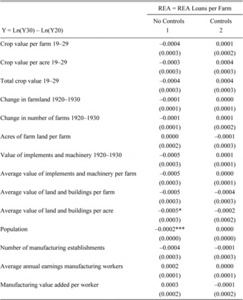
To measure the impact of the REA loans, we develop a new panel data set for the 1930s with information on the REA loans, other New Deal programs, and a wide range of socioeconomic measures: population growth, agricultural output and productivity for multiple products, land values, and the use of labor and machinery on farms.Footnote 3 The impact of the REA is identified using variation within counties over time and controls for the primary form of selection used by the REA in choosing projects, distance from the existing electric grid in 1935. Because electricity delivery costs to more distant areas were high enough that the longer distance projects could not succeed, REA officials distributed the loans to projects that were closer to the existing electric grid seeking to ensure that the loans would be repaid. Placebo tests suggest the absence of selection bias in our analysis by showing no relationship between the distribution of REA loans and changes in economic outcomes in the 1920s.
The REA was introduced into rural economies that in many cases had not yet recovered to their 1929 levels. We find that the loans substantially contributed to a rise in overall crop output, crop output per farm, and crop output per acre. In addition, the REA loans helped stave off longer run declines in the number of farms, overall output on farms, and the value of land and buildings on farms. Given the tight focus of the REA on electrifying farms and the disruptions in labor markets during the Great Depression and the New Deal, the effects on nonagricultural parts of the economy were generally small.Footnote 4
THE RURAL ELECTRIFICATION ADMINISTRATION
By 1930, almost every major city and town in the Unites States was electrified.Footnote 5 In 1932, domestic service in towns and cities accounted for 80.8 percent of all electric consumers nationwide, yet farm service only accounted for 2.6 percent of all customers (U.S. Census Bureau 1934). The share of farms with access was slightly higher; in 1925, 3.2 percent of farms had electricity with 10 percent by 1930. By 1950, more than 90 percent of farms had electricity.
On 11 May 1935, Executive Order 7037 created the REA and extended the scope of the Emergency Relief Appropriation Act to include rural electrification projects. Between 1935 and 1939, the REA handed out the equivalent of 0.3 percent of gross domestic product (GDP) in government subsidized loans to newly formed cooperative utilities and existing private utilities to provide access to electricity in rural areas. By 1940, more than 250,000 miles of line had been constructed connecting more than 956,000 farms, more than doubling the number of farms receiving service as of 1935 (Slattery Reference Slattery1940).
The REA provided 25 year loans at interest rates pegged to the long term U.S Treasury bond. REA rates fluctuated from 2.69 to 3 percent at a time when most loans of this type charged 6 percent interest (Slattery Reference Slattery1940).Footnote 6 The typical REA project required $230,000 (3.6 million in 2010 dollars) in loans to construct 250 miles of rural distribution lines to connect about 800 customers. Roughly 75 percent of these customers were farms. The rest were schools, churches, general stores, and small shops.
When deciding how to allocate the loans, the REA carefully scrutinized the fiscal soundness of applicants. Administrators paid particular attention to the terms the wholesale power distributers gave to these small electric cooperatives, as wholesale power costs represented approximately 75 percent of the total payments made by loan recipients. As the REA noted,
“In terms of the feasibility of projects, the power cost is the largest item of cost in connection with their operation…. We have taken the position that if a proposed wholesale rate for any project, taking into account variable conditions, is not such as to make an otherwise good project economically feasible and self-sustaining, REA cannot make a loan.” (REA 1938b).
“Sometimes a difference of a fraction of a cent per kilowatt hour in the wholesale rate will represent the difference between a sound and unsound project.” (REA 1937, 1938b; Slattery Reference Slattery1940)
The REA actively rejected applications that could not secure a favorable wholesale rate, or contracts that contained exclusive territory clauses that might restrict the cooperative's future growth (Richardson Reference Richardson1961). In what follows, we use the relationship between wholesale electric rates and the allocation of REA loans to inform our empirical strategy.
Both before and during the execution of the loan, the REA provided valuable assistance to potential applicants and loan recipients.Footnote 7 The REA provided groups of farmers interested in setting up a cooperative utility information regarding the legal steps required to establish such a utility, helped pass enabling state level legislation and regulatory policies, combated propaganda created by private utilities, developed methods to acquire rights-of-way, and provided accounting and management training to cooperative employees. The REA also pushed the technological frontier in electric distribution by developing construction methods that reduced costs per mile from $2,000 to $850.
The REA, perhaps naturally, promoted the benefits of electrification on the farm, both in the field and in the home. By 1938, the REA reported more than 200 uses for electricity on the farm, highlighting electricity's use in a variety of applications, such as cooled milk storage and spray irrigation. All of these innovations allowed more to be produced with fewer inputs while products became more consistent and of higher quality. At the agricultural experiment stations, for example, electricity increased the profitability per hen by 23 cents in Missouri and 53 cents in Alabama. The REA also showcased the improvement in amenities associated with electric lighting, pumped water, heated water, electric stoves, electric irons, washing machines, and other household appliances. For the average family of five, more than 300 hours and 350 miles of walking per year could be eliminated by installing an electric water pump. All of these goods improved the quality of life for rural residents.
THEORETICAL FOUNDATIONS
Access to electricity potentially led to several changes in rural areas. To provide a framework for discussing these changes, we use a model developed by Jennifer Roback (Reference Roback1982), and used more recently by Michael Greenstone, Richard Hornbeck, and Enrico Moretti (Reference Greenstone, Hornbeck and Moretti2010) to examine how electrification changed the profitability of firms (or farms in our case) in a given location. In the model, there are two locations, farms in each location have a production function with a location specific productivity parameter, A. The farms use labor (L), capital (K), land (T), and energy inputs (E) to produce a single internationally traded good with the price normalized to 1. The farms in each location maximize the following profit function

The input prices are w for labor, r for capital, q for land, and s for energy. From the first order conditions, farms choose the profit-maximizing levels of each input as a function of the factor prices. For instance, E ∗(A,w,r,q,s), is the optimal use of energy in a given location.Footnote 8
To understand the impact of the REA, we allow the productivity parameter and local input prices to depend on access to REA electricity. To summarize all of the effects that electric access has on firm profits in the short run, we take the total derivative with respect to access at their optimums. After collecting terms and allowing inputs to be paid their marginal product this exercise yields the following expression

Equation (2) shows that the REA electrification affects farm profitability through four main channels. Access to the REA increases profits through increased farm productivity, lowers profits by raising wages, decreases profitability by increasing land prices as farms and workers compete for land, and raises profits as a result of lower energy prices. The overall impact on the REA is ambiguous because it is unclear if productivity gains and lower energy prices will be offset by more expensive labor and land. Therefore, empirical analysis of a variety of measures of farm and nonfarm activity is necessary to determine the net effects.
SAMPLE CONSTRUCTION
Data for the empirical exercise are derived from a variety of federal publications. Outcome and control variables come from Census publications compiled in Michael Haines (Reference Haines2005) and a new agricultural dataset collected by Price Fishback, Michael Haines, and Paul Rhode (Reference Fishback, Haines and Rhode2012). Data pertaining to the value of REA loan contracts by county, as well as other New Deal Agency loans are from Fishback, Shawn Kantor, and John Wallis (Reference Fishback, Kantor and Wallis2003), which originally came from unpublished mimeos of the Office of Governmental Reports (1939). Information detailing the location of REA projects comes from the Report of the REA (1939a). Because REA loan information at the county level is only available through 1939, the empirical exercise will focus on the period between 1935 and 1940, when the REA loan program was most active.Footnote 9
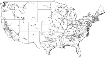
Data about the state of the electric grid prior to the formation of the REA is important in controlling for selection of projects based on access to the grid. The locations of the electric transmission grid and electric generation plants in 1935 come from the Federal Power Commission National Power Survey Interim Report Power Series No. 1 (1935a) and were digitized using ArcGIS and form the basis of measures of proximity to electric generation and transmission infrastructure (Figure 1).
1935 ELECTRIC TRANSMISSION GRID IN UNITED STATES

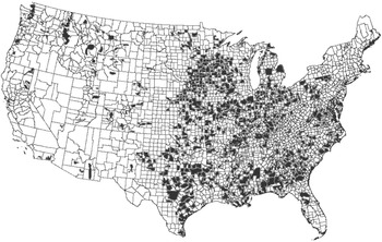
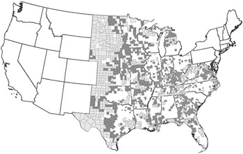
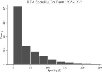
Figure 2 displays the service areas of the REA funded projects as of 1939. Most of the projects were located in the Mid Atlantic, Southeast, Great Lakes, and Midwest; so, we restrict the sample to counties in these states.Footnote 10 The sample is restricted further to counties with populations under 20,000 as of 1930 to eliminate large cities, which were not eligible for funding under the REA guidelines. Of the approximately 3,000 counties in the United States, the restrictions leave us with 1,377 counties in the sample shown in Figure 3. Counties shaded in light grey represent control counties, while counties shaded in black represent treatment counties. To construct our measure of treatment intensity, loans per farm, we use the total value of all REA loans to cooperative utilities in the county from 1935–1939 divided by the number of farms in 1929. For treated counties, the average loan value per farm widely varied. Figure 4 shows the distribution of REA loan value per farm from 1935 to 1939. The majority of counties, however, did not receive any funding. Conditional on obtaining loans from the REA, loans in the average county were $77 per farm.
SERVICE AREA OF INDIVIDUAL REA FUNDED PROJECTS 1939

COUNTIES IN SAMPLE

DISTRIBUTION OF REA LOANS PER FARM 1935–1939

While our empirical analysis focuses on changes between REA and non-REA counties from 1929 to 1939, it is useful to highlight initial differences between counties in 1929. Counties that were granted REA loans tended to have larger populations and had more, but smaller, and more productive farms than counties not receiving loans. Because there were more farms and output per acre was higher in the REA counties, mean total output, measured as value of farm products, sold, traded, or used and deflated by the wholesale price index for farm products was higher in the counties receiving REA loans in both 1929 and 1939. These two factors offset the lower value of output per farm in the REA counties, which was driven by average acreage that was about one-fourth of the average in the non-REA counties. Farms in REA counties tended to have lower shares of value devoted to animal products, at the same time using a higher share of their production on their own farm. The levels of inputs also varied, as farms in REA counties had higher land and building values (deflated by the wholesale price index for farm products) and lower values of farm machinery and implements (deflated by the wholesale price index for farm machinery) despite having less acreage. The farm operator worked fewer days off of the farm and used more family labor and less hired labor in the REA counties. These differences in the features of the REA and non-REA levels of activity led us to control for the starting level of key economic variables as well as to perform the placebo analysis described in the robustness section.
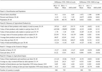
Table 1 summarizes the changes in outcomes experienced in both REA and non-REA counties from 1929 to 1939. It is important to realize that the comparisons that follow are made between a peak economy in 1929 and an economy in 1939 still recovering from the ravages of the Great Depression. The counties that received REA loans did better during the Great Depression than the counties that did not. The total value of farm products, the value per farm, and value per acre all fell in both types of counties between 1929 and 1939; however, the REA counties experienced smaller declines. While both types of counties produced a higher value of animal products and tended to use more of their output on their own farms, the average increase was larger in the REA counties. The value of land and buildings per farm deflated by farm product prices fell by roughly the same amount in both types of counties, while the value of farm implements and machinery per farm fell much less in the REA counties. Farm operators in both REA and non-REA counties increased their average days worked off of the farm by nearly 30 days, but the rise was lower in the REA counties. Between 1935 and 1939 farms in both types of counties used more hired labor and less family labor but the REA counties increased their use of hired labor less and reduced their use of family labor less. The population grew in both the REA and non-REA counties but grew by more people in the REA counties. The share of the rural farm population dropped in both counties but by less in the REA counties, suggest less movement off of the farm there. These summary statistics show the associations between the REA and the various dimensions of economic activity. The analysis that follows examines whether these same relative changes are present after controlling for a broad range of correlates. To the extent that these correlates control for all relevant factors, we can assign a causal role to the REA.
SUMMARY STATISTICS 1930–1940

Sources:
See text.
EMPIRICAL STRATEGY
When evaluating the effects of large infrastructure projects, researchers must carefully consider the fact that the programs often have specific goals, and are therefore, not placed randomly. In regards to the REA, we may be concerned that the administrators were either positively or negatively selecting locations that would either be the most able to repay the loans, or that were most likely to experience growth as a result of electrification. Thus, ordinary least squares (OLS) estimates that do not control for this selection process may suffer from omitted variables bias. In the growing literature that evaluates the rollout of electric infrastructure projects, previous studies have relied on variation in the cost of installing infrastructure associated with differences in topography or the cost minimizing placement of long lived generation equipment (Dinkleman Reference Dinkelman2011; Grogan and Sadanand Reference Grogan and Sadanand2013; Lipscomb, Mobarak, and Barham Reference Lipscomb, Mobarak and Barham2012; Kitchens Reference Kitchens2014). Given that agricultural outcomes are often correlated with topography, these types of geographic-based instruments are unlikely to satisfy the exclusion restriction.Footnote 11 For instance, one may suspect that the land gradient (a common instrument) is correlated with the adoption of the tractor, or improvements in transportation networks. Further, being closer to the grid may also mean that the farms are closer to more population dense areas that would confer the advantages of being closer to markets. All of these factors likely affected the types of crops planted (affecting the value of crops), land values, and population movements.Footnote 12 Because of these empirical problems, we rely on the historic narrative to address the potential endogeneity problem by directly including variables that the REA considered when selecting which projects to fund, namely, the proximity of the project to existing electric transmission and generation infrastructure.
Our empirical strategy relies on a differences-in-differences approach to identify the reduced form effect of REA electrification on a variety of outcomes related to agricultural productivity and the use of agricultural inputs. To further examine whether the REA results might be considered causal, we present two additional types of evidence. First, we present a set of placebo regressions to evaluate whether or not pre 1930 trends affected where REA funds were disbursed. Second, we discuss how large selection on unobservables would have to be to invalidate the direction of impact of the REA using a framework developed by Joseph Altonji, Todd Elder, and Christopher Taber (Reference Altonji, Elder and Taber2005) and extended to an OLS framework by John Bellows and Edward Miguel (Reference Bellows and Miguel2009).
Empirical Specification
We examine the influence of the REA by using information on the dependent variables from two years: one before the REA was put into effect and the other just as the first round of REA loans were made (1 July 1935 and 30 June 1939) had ended. The year prior to the REA year is either 1929, 1930, or 1935, while the REA year is either 1939 or 1940. For simplicity in the discussion of the empirical model we will use 1930 and 1940 to designate the two years. Had REA loans been randomly assigned, the average treatment effect of a REA loan can be estimated with the following OLS regression:

ln Y it is the natural log of the dependent variable in county i and year t—either 1930 or 1940. D40 is a dummy variable with value 1 in 1940 and zero in 1930. The value of REA loans in the given county in the specified time period is given by REA it . The variable takes on the value of zero in 1930 and the cumulative value of loans between 1 July 1935 and 30 June 1939 per farm in 1940.Footnote 13 The vector X i,30 contains a variety of pre-treatment correlates measured prior to the introduction of the REA. We allow the pre-treatment correlates to have differential effects in 1930 and 1940 by interacting X i,30 with the 1940 dummy, such that β 30 measures the impact of the X i,30 correlates in 1930 and β 40 measures the difference in the impact of the same correlates in 1940. The baseline characteristics in a pre-treatment year are used rather than the levels of observed characteristics in 1940 because electricity is a general purpose technology, which likely affected many outcomes simultaneously. Therefore, for each outcome, the REA coefficient measures the sum of all of the effects on that outcome in 1940 that might have operated through a variety of outcome measures, while controlling for the prior levels of a rich set of covariates.
In addition, we control for grants and loans from other New Deal programs in the vector ND3339, so that we are not ascribing effects to the REA that actually were the result of other New Deal programs. The New Deal measures include Agricultural Adjustment Administration (AAA) grants per farm, Farm Security Administration (FSA) loans per farm, Farm Credit Administration (FCA) loans per farm, other non-farm New Deal grants per farm and other non-farm New Deal loans per farm. Finally, to control for time-invariant unobservable characteristics in the counties, we include a vector of county fixed effects, μ i .
We estimate the model in first differences. After subtracting the equation for 1930 from the equation for 1940, and making adjustments, the final equation for estimation is

The equation takes this final form because the α 0 , β 30 X i,30 and μ i terms are the same in both years. Because D40 is zero for the 1930 equation and one for the 1940 equation, α 1 and β 40 X i,30 is the outcome of the first difference for the terms where D40 appears. There were no REA loans or New Deal programs in 1930, so the first difference is the level value for the REA for 1935 through 1939 and the New Deal levels for 1933 through 1939. The model controls for potential endogeneity arising from pretreatment differences in the counties and time-invariant features of the counties, while also controlling for spending and loans in other New Deal programs. However, it is possible that REA funds were directed to locations with differential pre-trends, which we will test for below.Footnote 14
Even with these controls in place, we take additional steps to control for selection bias that might arise because the REA paid close attention to the location of the grid in making decisions on where to place loans and because distance to the grid was likely correlated with unmeasured geographic and market features that would have influenced agricultural outcomes. The narrative analysis of the REA decision process shows that the dominant factor determining the location of REA loans was the potential cost of distributing electricity, which was strongly correlated with the distance from the existing electricity grid.Footnote 15 To control for this selection process, we include two additional covariates that strongly affected the cost of obtaining electric service, the distance to the nearest generation station and the distance to the nearest transmission line. Greater distance along distribution lines meant more load loss due to resistance in the transmission lines and thus greater cost of delivering electricity.
The REA explicitly included these costs as a major component of their decision to grant loans to applicants. Both the proximity to central electric stations and to large transmission networks influenced the costs of delivering electricity, and thus, the financial success of loan applicants. These cost differentials were potentially very large; in 1935 the Federal Power Commission reported those distribution losses ranged from 10 to 40 percent of all power sales in the country (FPC 1935b). In regressions of REA loans per farm as a function only of the two distance measures and a constant, a one standard deviation (OSD) increase in distance from a generation plant leads to a 0.12 standard deviation decrease in REA loans per farm. For an OSD increase in the distance from the transmission grid, REA loans per farm falls by 0.079 standard deviations. Combined, these variables explain 3.3 percent of the variation in REA loan value per farm.
The Impact of the REA
When discussing the impact of the REA, it is important to recognize that that population was growing in both in treatment and control counties and that a decade of depression and slow recovery meant that the economies in these counties were in worse shape than they had been in 1929. Thus, when we are discussing positive coefficients for the REA, in many situations the REA counties performed better relative to the non-REA counties at promoting recovery or attenuating declines.
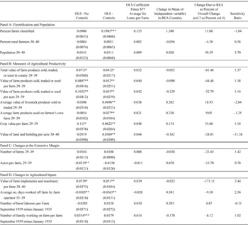
Before discussing the impacts of the REA on agricultural outcomes, we first want to highlight the fact that the REA did indeed increase rural electrification rates. The changes highlighted in Table 1 show that electrification grew faster in REA counties than non-REA counties. However, it is likely that the REA stimulated activity among private firms that sought to keep the rights to exclusive territories. This competitive behavior was strong enough, that in some instances approved REA projects had to be abandoned (Neufeld Reference Neufeld2015), thus, any estimate of the REA's impact is likely to underestimate its true effect. Despite these empirical problems, we find that the REA had a positive and statistically significant impact on the farm electrification rate. In Table 2, Panel A, we show that for every $100 in loans, the REA increased rural electrification by 0.1985 log points. At the mean loan per farm, the REA loans increased farm electrification rates by 0.153 log points. Between 1930 and 1940, the average rural electrification rate in REA counties increased by 1.38 log points, thus, REA accounted for 11.08 percent of that increase.
MAIN RESULTS Y = LN(Y40) – LN(Y30)

Notes:
Each entry in this table comes from a separate regression. Coefficients and standard errors are scaled by 100. Robust standard errors clustered at the state level are in parentheses. New Deal control variables are for the period 1933 through 1939: AAA Spending per farm, FSA and FCA Loans per Farm, New Deal Grants per farm, and New Deal loans per farm. The number of farms and population are from 1930. The other control variables are from 1930 (or other year) and are the population, percent in manufacturing of gainful workers, number of farms, percent of the population illiterate, the percent unemployed, the number of farms, the percent black, percent married, percent divorced, percent foreign born, percent of acres operated by tenants, per capita crop value (1929), and percent owning a radio. ∗ indicates p<0.1, ∗∗ indicates p<0.05, *** indicates p<0.01.
Sources:
See text.
REA loans contributed to increases in the value of crop output, and helped offset declines in overall agricultural output and productivity per acre. Each entry in columns 1 and 2 of Table 2 shows the coefficient from a separate regression using the value of REA loans per farm as the measure of REA access. For readability, we scale the coefficient by 100 so that the coefficients can be interpreted as percentage points. Robust standard errors clustered at the state level are reported in parentheses.Footnote 16 We will focus on the results with the full set of pre-treatment controls in discussing the magnitudes of the effects since these estimates are less likely to be affected by omitted variable bias and endogeneity bias.
The trends in the summary statistics (Table 1) show that the total value of farm output declined between 1929 and 1939. The introduction of the REA into a county helped stave off this decline relative to the non-REA counties through a complicated set of interactions stimulating the value of output per farm and the value of output per acre. The most comprehensive measure of farm output is the real value of farm products sold, used, and traded per farm, which we deflated by the wholesale price index for farm products.Footnote 17 The authors of the 1940 Census considered this measure to be their closest approximation to gross farm income (U.S. Census Bureau 1943, p. 869). In Table 2, Panel B, the coefficient of the REA loans per farm is 0.0412, which implies that a one dollar increase in REA loans per farm raised the total value of farm products, sold, traded, or used in the county by roughly 4 percent. The mean REA loan per farm in REA counties of $77 was associated with a change in the natural log of the value of farm output of 0.032 log points, which can be compared with a decline in the mean log value of output of –0.052 log points in REA counties. This finding suggests that without the REA the mean natural log of the value of output would have fallen by –0.084 log points rather than the decline of –0.052 log points with the mean REA loan in place. Thus, the REA loan helped prevent an additional 61.4 percent of the actual decline.
The positive effect of the REA loans was driven largely by an increase in the value of farm products per farm and per acre, yet having no statistically significant impact on the number of farms or farm size. Here again, the productivity increases associated with the REA worked to offset downward trends between 1929 and 1939. In the summary statistics for REA counties (Table 1) both the value of farm products, sold, traded, or used per farm and the same value per acre fell by 9 and 13 percent, respectively, between 1929 and 1939. The REA loan coefficients imply that the $77 average REA loan per farm was related to a rise of about 4.0 to 4.2 percent of the value of output per farm and per acre. Thus, without the REA the value of output per farm likely would have fallen by 13 percent, or about 44.5 percent more than the decline that actually occurred. Similarly, the average REA loan per farm would have raised the value of farm products per acre by 4.2 percent compared with a drop in the mean value of 12.9 percent with the REA loan in place; therefore, the REA loan helped prevent an additional 32.8 percent drop in the mean value of farm products per acre. The impact of the REA on the value of farm products arise while controlling for other New Deal programs targeted at agriculture, such as the AAA, that provided aid to farmers to take land out of production, which also were considered to have raised output per acre but encouraged larger farm sizes (Depew, Fishback, and Rhode Reference Depew, Fishback and Rhode2013). We note that the increases in output are not driven by increases at the extensive margin. In Table 2, Panel C, we show that the REA loans did not have statistically significant relationships with the changes in the number of farms or the average acreage per farm.
The REA loans were associated with increases in the value of output per farm across several dimensions, the value of crop output, the value of animal products, and the value of farm products used on the farmer's own farm. We constructed measures of county level crop values using the county level crop output figures multiplied by estimates of county prices, deflated by the wholesale price index for farm products.Footnote 18 The coefficients in Table 2, Panel B, suggest that the introduction of the mean REA loan would have accounted for 35.6 percent of the rise in crop value per farm between 1930 and 1940.
The REA loans were also associated with increases in the real value of livestock products sold or traded per farm and in the per farm value of farm products used on the farmers' own farm. A move from no loan to the mean REA loan per farm contributed 18.9 percent of the rise in the mean value of livestock products sold or traded per farm and 9.05 percent of the rise in mean products used by the farmer on his own farm.
The REA's stimulus of the value of output per farm and per acre helped offset a decline in the value of the land per acre and the value of land and buildings per acre between 1930 and 1940 in REA counties. The Census reported estimates for both. The agricultural reporters, however, were not convinced that the separate estimates for the value of buildings and the value of land that they received were as good as the estimates of the combined value of land and buildings because the purchase price of most farms was the combined value of both land and buildings (U.S. Census Bureau 1943, volume 3, p. 27). The REA coefficients imply that the REA loans led to increases in the values of land and buildings per acre that worked to offset the overall decline.Footnote 19 In the absence of the average REA loan the mean natural log of the value of land and buildings per acre would have fallen by –0.226 log points. This fall would have been 24 percent more than the actual 0.182 log point fall.
Contributing to the positive relationship between REA loans and output per acre was an increase in the real value of farm implements and machinery per farm whose values were deflated by the Wholesale Price Index for farm machinery. The REA loans slowed a trend toward less use of machinery. Between 1930 and 1940 the mean natural log of the value of machinery per farm fell by 2.3 percent in the REA counties (Table 1). However, the REA loan coefficient for machinery shows that with no REA loans the mean value of machinery per farm would have fallen by 6.2 percent; thus, without REA loans the decline that would have been 171.11 percent more negative.
The REA stimulus to farm activity led to a change in the use of labor inputs on farms. In counties receiving the average REA loan per farm, farm operators reduced the number of days they worked off of the farm by about 3 percent, which worked against a 30.1 percent rise in the mean days worked off the farm between 1935 and 1939. The REA loans possibly increased the use of family labor and hired labor on the farms, but the REA loan coefficient was statistically insignificant in each case.
Despite the rise in the real value of output per farm, the REA loans appear to have had little impact on population changes in the county. The REA loan coefficients in the population were positive, and the population coefficient implies that the mean REA loan would have contributed 30 percent to the rise in average population in REA counties, but none of the coefficients were statistically significant.
Possible Selection on Unobservables
While our empirical strategy addresses endogeneity arising from differences in the initial level of the outcome, it is possible that funds were directed to locations on differential pre-trends or unobservables. To test the effectiveness of our design and control variables, we estimate a set of placebo regressions by examining changes in outcomes from 1920 to 1930, a period well before the creation of the REA, as a function of REA loans per farm.Footnote 20 The results of this exercise are presented in the Appendix and show that the allocation of REA funds were not correlated with pre-treatment trends.
While our placebo tests suggested that REA loans were not directed towards counties on the basis of the pre-trends, there still might be a possibility that the 1920s decade was structurally different from the 1930s decade in ways that we have not controlled for with all of the correlates included in the analysis. If true, the placebo tests might not fully rule out selection bias. It is not clear how large that uncontrolled difference would be. The biggest change in rural areas in the 1930s was driven by the introduction of the New Deal farm programs and the emergency public works and relief spending, and we control for these dramatic changes by incorporating measures of the programs in our analysis. In addition, we have examined national trends in agriculture over the 1920s and 1930s in number of farms, farm populations, farm price indices, average farm sizes, and measures per farm of the value of farm machinery, farm trucks, farm autos, and tractors. The series either follow similar trends in both decades, no trend, or no clear change in trend.
To examine further the issue of potential omitted variable bias, we suggest an alternative way to evaluate the likelihood that our estimates are biased by omitted variables correlated with the REA and the outcomes. Following the work of Altonji, Elder, and Taber (Reference Altonji, Elder and Taber2005), henceforth AET, and extended by Bellows and Miguel (Reference Bellows and Miguel2009), we construct sensitivity ratios that suggest that if the estimates are not sensitive to the inclusion of observables, then they are also unlikely to be influenced by the inclusion of unobservables.
In an AET framework, the set of observable explanatory variables, X, is a random subset of the full set of explanatory variables, Z. If a researcher only includes observable X variables, the estimated coefficient, β
C
, will be the true parameter value, β
True
, plus any remaining omitted variables bias after the inclusion of X. In the absence of covariates, X, then the estimate, β
NC
, would be the true parameter value plus all omitted variable bias. If the coefficients between these two sets of estimates differ little, it would suggest that there is very little omitted variables bias. Furthermore, because the X's are randomly drawn from Z, it is unlikely that the addition of other variables from Z not contained in X would further affect the estimates. As a rule of thumb, AET suggest that the estimates should have a sensitivity ratio greater than one, where the sensitivity ratio is defined as  . Using this formulation, we do not need to worry about selection on unobservables if the coefficients are not diminished by more than one-half upon the inclusion of controls.
We report the sensitivity ratios in the far right column of Table 2. The sensitivity ratios are greater than one for 13 out of the 16 outcomes. The outcomes for which the sensitivity ratio is less than one were ones that we have not emphasized in the discussion because the coefficients were typically statistically insignificant as well. Combined with the set of placebo regressions, which indicated that REA and non-REA counties were on similar trends prior to the creation of the REA, we believe that it is plausible that REA funds were randomly distributed conditional on our set of controls. Therefore, the reported estimates might be considered causal.
Robustness Checks
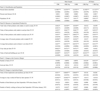
In our main specification, we restricted the sample in two ways. First, we imposed a population threshold of 20,000, and we excluded states in the Northeast and West. In what follows, we test the robustness of our results to these arbitrary sample restrictions. First, we relax the population threshold by re-estimating the model for a different set of population thresholds: 40,000 and 100,000. Second, we relax the restriction on the set of states included. The results from this specification are presented in Table 3. In each specification, we include the full set of covariates and cluster the standard errors at the state level. We present our baseline results in column 1 as a reference for the reader.
ROBUSTNESS SPECIFICATIONS – SAMPLE RESTRICTIONS

Notes:
See notes from Table 2.
Sources:
See text.
In column 2, we present the results when the sample includes all counties with under 40,000 in population. In column 3, we present the results from the inclusion of locations with less than 100,000 in population. This evidence makes it clear that the results are not driven by sample selection arising from our imposed population cutoff. In Column 4 we present the results using all counties in the United States with a population under 20,000. In general, the results have the same sign as our baseline results, however, the Northeast and West were not typically candidates for the program and thus more dissimilar from the areas where the REA was instituted.
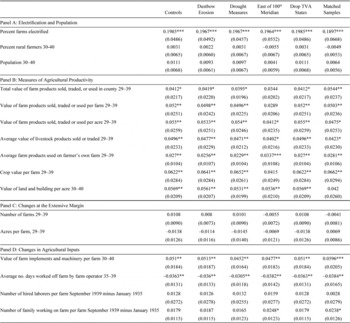
In addition to these changes in sample specification, there may be other concerns. First, a large portion of our sample lies in the Great Plains, which experienced a major ecological change due to the Dustbowl. Failure to account for the changing conditions in the Plains might bias our estimates of the REA's impact. We address this concern in three ways: (1) we include measures of the Dustbowl's impact on erosion by including the Dustbowl severity index utilized by Zeynep Hansen and Gary Libecap (Reference Hansen and Libecap2004) and Richard Hornbeck (Reference Hornbeck2012), (2) we include measures of the Palmer Drought Severity Index, annual precipitation, and annual average temperature, and (3) we drop all counties in the sample west of the 100th meridian.Footnote 21 The results of these specifications are reported in Table 4, columns 2–4. All are qualitatively similar to our baseline specifications, mitigating concern that the Dustbowl is influencing our main findings.Footnote 22
ROBUSTNESS SPECIFICATIONS II – DUST BOWL AND TVA

Notes:
See Notes to Table 2. Additionally, each specification reported in this table examines a specific sub-sample or includes additional covariates. Columns 1 replicates our baseline results, reporting the coefficients with the inclusion of covariates. Columns 2–4 address different concerns regarding the Dustbowl. Column 2 includes the Dustbowl measures used by Hansen and Libecap (Reference Hansen and Libecap2004), which uses a set of dummies to denote the severity of erosion. Column 3 replaces these measures with the Palmer Drought Severity Index for 1930–1932 and the average temperature and average precipitation in the county. Column 4 drops counties west of the 100th meridian. Column 5 excludes counties located in Alabama, Mississippi, and Tennessee, which encompasses the service territory of the TVA in 1940. Finally, in column 6 we report results from a specification where we drop counties with a propensity score less than 0.4, where the propensity score is estimated by relating an indicator variable of the REA with the pre-treatment X variables.
Sources:
See text.
A second concern is that several of our REA cooperatives are located within the service territory of the Tennessee Valley Authority (TVA). While Carl Kitchens (Reference Kitchens2014) showed that the TVA had little impact on rates charged to consumers, the TVA's presence may affect our results if it helped facilitate coordination with potential lenders. To address this concern, we drop all counties located in Alabama, Mississippi, and Tennessee, because these are the states where the TVA had electricity contracts as of 1940. The results of this specification are presented in column 5 and are qualitatively similar to our baseline results, alleviating concerns that we have confounded the effect of the REA with the TVA. Finally, in column 6, we report the results of a specification where we drop counties that were unlikely to receive funding from the REA based on a pre-treatment propensity score estimate and find results that are qualitatively similar to our baseline specification.
DISCUSSION
The REA was different from many other electrification projects. First and foremost, it was a loan program that focused on the construction of distribution lines and connecting customers rather than direct investment in grid infrastructure and generation. It also worked closely with loan applicants to design a system that would be financially successful and minimize the risk of default.
Some of the benefits, such as the in-kind benefits the REA provided applicants through improvements in state legislation, wholesale contract negotiations, management training, and engineering advice, are difficult to directly quantify, however, it is possible to measure the interest subsidy. If cooperatives had been able to acquire loans privately, the interest rate would have been at least 6 percent; however, REA loan interest rates were set at approximately 3 percent, to be amortized over 25 years (Slattery Reference Slattery1940).
The average REA loan contract was for a principal of $230,000 amortized over 25 years at an interest rate of approximately 3 percent, with monthly payments of $1,090.69. The average farm mortgage rate was around 5 percent between 1935 and 1940, which would have led to monthly payments of $1,344.56. Assuming that farm cooperatives or commercial entities obtain the 5 percent interest rate, the ex ante interest subsidy at the time the REA loan was made would have been the difference in the present value of the two streams of 300 monthly payments when evaluated at 5 percent. The estimated subsidy on the loan would have been $43,389, which was 18.9 percent of the principal on the loan. The actual ex ante subsidy was lower to the extent that cooperatives and firms could obtain lower interest rates than for farm mortgages, but it might well have been higher if interest rates reached Slattery's estimates of 6 percent if the electrification projects were considered to be riskier. This ex ante subsidy is comparable in percentage terms to the size of the ex ante subsidies for the purchase and refinance of one million nonfarm mortgages by the Home Owners' Loan Corporation (HOLC) found by Fishback, Jonathan Rose, and Kenneth Snowden (2013). Footnote 23
Ex post, the REA loans had a much better record of repayment than the HOLC loans. The HOLC ended up foreclosing on 20 percent of their refinanced nonfarm home loans, although the overall losses from the HOLC ended up at about 2 percent of the value of the loans refinanced. In contrast, almost all REA loans from the 1935 to 1939 period were repaid, minimizing the ex post costs to the government. As of 31 December 1942, 3 percent of borrowers were behind on interest payments, 0.7 percent were behind on principal payments, while 37 percent of loans had been repaid in full, and another 53 percent were ahead of schedule on principal repayments (USDA 1943).Footnote 24 This contrasts with figures for the HOLC in which one-third or more of borrowers were more than 3 months behind on principal and interest payments as late as 1940, seven years after the start of that program. Given the speed at which loans were repaid, and the relatively low default rates, the government's primary expenditure came through its engineering services, advising, and management training.
CONCLUSION
Electrification has been a central policy tool in developing countries as nations look to invest in infrastructure. Several nations are currently seeking billions of dollars to extend and make their infrastructure more reliable to attract firms and promote growth. We show here that the during the period 1930–1940 the REA's extension of loans to cooperatives to electrify farms led to large productivity improvements in agriculture, which in turn led to increases in land values. To identify the effect of the REA on economic outcomes we use within county variation over time while controlling for selection by including measures of cost associated with access to grid infrastructure, and then performing placebo test that suggest a lack of selection bias.
We find that during the period 1930–1940, the introduction of the REA led to increases in agricultural productivity, which led farmers to seek employment off the farm less often, and increased property values. The REA made rural life more attractive by increasing productivity on the farm and improving amenities in the home. As developing nations introduce electric grids to urban and rural areas, there are likely to lead to similar changes in those countries, although there might be more of a migration and population growth response than we found.
Appendix
PLACEBO REGRESSIONS