1 Introduction
The gravity-driven flow of a viscous liquid film down an inclined plane, or even a vertical plane, is an important problem with many industrial applications such as coating processes (paints, varnishes, printing inks
 $\ldots$
) or in chemical reactors, absorption columns, condensers and evaporators. The flat film solution with a parabolic velocity profile, called Nusselt flow, can become unstable for sufficiently high slopes against long-wavelength infinitesimal perturbations. When the Nusselt flow is unstable, trains of travelling waves can appear. High-frequency disturbances evolve to saturated periodic waves whereas low-frequency disturbances lead to waves sufficiently far away one from each other to be assimilated to a succession of solitary waves. Such a solitary wave has a main hump preceded by many smaller capillary ripples. For this long-wavelength interfacial instability, viscosity and surface-tension effects are important. For some applications such as coating processes, a uniform flow thickness is required. In this case, the instability should be avoided. For processes in chemical engineering, the instability can be sought as the interfacial waves enhance heat and mass exchanges.
The first experimental and theoretical studies were due to Kapitza (Reference Kapitza1948a ,Reference Kapitza b ) and Kapitza & Kapitza (Reference Kapitza and Kapitza1949). The instability threshold was found by Benjamin (Reference Benjamin1957) and Yih (Reference Yih1963) with a power expansion of the Orr–Sommerfeld equation. A direct numerical simulation of the Navier–Stokes equations is very difficult and has a high computational cost because of the dimensionality of the problem and the existence of a free surface. However several results have been obtained (Bach & Villadsen Reference Bach and Villadsen1984; Salamon, Armstrong & Brown Reference Salamon, Armstrong and Brown1994; Ramaswamy, Chippada & Joo Reference Ramaswamy, Chippada and Joo1996; Malamataris, Vlachogiannis & Bontozoglou Reference Malamataris, Vlachogiannis and Bontozoglou2002; Nosoko & Miyara Reference Nosoko and Miyara2004; Trifonov Reference Trifonov2012) mostly in the two-dimensional case. An intermediate level of modelling is given by the boundary layer equations (Demekhin, Demekhin & Shkadov Reference Demekhin, Demekhin and Shkadov1983; Chang, Demekhin & Kopelevich Reference Chang, Demekhin and Kopelevich1993) which are derived by assuming that the streamwise variations are small by comparison with the crosswise variations. The resulting equations are in effect reduced Navier–Stokes equations which are simpler than the full Navier–Stokes equations but with the same dimensionality. To get a reasonable computational cost, models of reduced dimensionality have to be derived. In most cases, the flow remains close to the Nusselt flow. This allows long-wave asymptotic expansions which form the basis of many models. By averaging the Navier–Stokes equations over the fluid depth, models of dimensionality reduced by one can be derived. In addition, as the boundary conditions are incorporated in the equations of the model, the numerical resolution is much simpler and faster.
A prerequisite of such a model is that it must capture the main physical features of the flow. Further, it is essential that the equations of the model can be easily numerically solved in order to get reliable solutions. The mathematical structure of the equations is thus a critical feature of a model since the numerical schemes used to solve the equations depend on their structure. For some well-known mathematical structures, reliable and robust numerical schemes have been developed and extensively studied.
One-equation models have been successfully derived after the seminal paper of Benney (Reference Benney1966). They provide consistent models in the limit of the long-wave asymptotic approximation. The single equation is an evolution equation for the film thickness
 $h$
. One-equation models of first order are scalar hyperbolic conservation laws and discontinuities arise in a finite time as soon as the critical Reynolds number of the Orr–Sommerfeld theory is reached. When using more accurate one-equation models such as the Benney equation, blow up of solutions usually arises when linear stability criteria are violated (Pumir, Manneville & Pomeau Reference Pumir, Manneville and Pomeau1983; Joo, Davis & Bankoff Reference Joo, Davis and Bankoff1991), except in the limit of small-amplitude modulations where the Benney equation degenerates towards the Kuramoto–Sivashinsky equation (Kuramoto & Tsuzuki Reference Kuramoto and Tsuzuki1976; Sivashinsky Reference Sivashinsky1977). This drawback was solved by Ooshida (Reference Ooshida1999) by using a Padé-like regularization technique but the wave solutions of the equation thus derived are not accurate except relatively close to the critical Reynolds number (Ooshida Reference Ooshida1999). It seems unlikely that a model with a single evolution equation for the fluid depth could describe completely and accurately the dynamics of waves in thin films down an inclined plane. In particular, it seems essential to relax the enslavement of the fluid velocity to the fluid depth and consequently to treat the velocity as a second variable of the model.
The first two-equation model for laminar film flows was proposed by Shkadov (Reference Shkadov1967). The variables of the model are the fluid depth
 $h$
and the fluid discharge
 $q$
(or equivalently the averaged fluid velocity
 $U$
). While this model can describe the waves that can appear in thin films flows, it is not consistent with the analysis of long wave expansion of the Orr–Sommerfeld equation. In the long-wave limit, this model gives the correct value of the critical Reynolds number only for vertical walls (where the Nusselt flow is unstable for all values of the Reynolds number) whereas the predicted instability threshold is incorrect for moderately inclined planes. In order to average the Navier–Stokes equations over the depth, the velocity profile is supposed to be the self-similar parabolic profile of the Nusselt flow even if this flow becomes unstable.
Several experiments showed that there are deviations from the parabolic profile in a solitary wave in thin film flows (Nakoryakov et al.
Reference Nakoryakov, Pokusaev, Alekseenko and Orlov1977; Alekseenko, Nakoryakov & Pokusaev Reference Alekseenko, Nakoryakov and Pokusaev1985). Numerical simulations (Bach & Villadsen Reference Bach and Villadsen1984; Malamataris et al.
Reference Malamataris, Vlachogiannis and Bontozoglou2002) found similar results. These deviations are relatively small (but nevertheless as high as 15 % according to Alekseenko et al. (Reference Alekseenko, Nakoryakov and Pokusaev1985)) except close to the front of the wave where considerable departures from the parabolic profile can appear. Several other models were proposed along the lines of Shkadov’s approach and some relaxed somewhat the self-similar parabolic profile assumption such as in Nguyen & Balakotaiah (Reference Nguyen and Balakotaiah2000) who used a more general parabolic profile and derived a three-equation model for the film thickness, the volumetric flow rate and the wall shear stress. Ruyer-Quil & Manneville (Reference Ruyer-Quil and Manneville2002) pointed out that the failure of the model of Shkadov and of attempts to cure its deficiency by adding higher-order terms or surface-tension corrections can be traced back to the lack of flexibility of the assumed velocity profile, either the simple parabolic profile or some other self-similar fixed profile function. Starting with an expansion of the velocity field in terms of polynomial test functions and using a weighted-residual technique based on a classical long-wavelength expansion, they derived first a two-equation model for the film depth
 $h$
and the flow rate
 $q$
, consistent to first order, and then a second-order four-equation model (Ruyer-Quil & Manneville Reference Ruyer-Quil and Manneville2000). This weighted-residual integral boundary layer model (called thereafter the RQM model) is a system of four equations for the variables
 $h$
,
 $q$
and two supplementary variables homogeneous to
 $q$
measuring the corrections to the parabolic profile. They also derived a simplified model with only two equations which is obtained when the two supplementary variables are supposed to be of a higher order than second (Ruyer-Quil & Manneville Reference Ruyer-Quil and Manneville2000). This two-equation model is still consistent with a long-wave expansion of the Orr–Sommerfeld equation and gives the correct critical Reynolds number. While the two-equation RQM model gives good results, especially by comparison with other two-equation models (Ruyer-Quil & Manneville Reference Ruyer-Quil and Manneville2005; Chakraborty et al.
Reference Chakraborty, Nguyen, Ruyer-Quil and Bontozoglou2014), the four-equation RQM model gives certainly the best results of all models to date. It was recently successfully compared to a direct numerical simulation (DNS) of the full Navier–Stokes equations (Chakraborty et al.
Reference Chakraborty, Nguyen, Ruyer-Quil and Bontozoglou2014). Its only drawback is that its mathematical structure is complicated and, consequently, its numerical resolution is difficult.
Mudunuri & Balakotaiah (Reference Mudunuri and Balakotaiah2006) assumed a self-similar parabolic velocity profile and used also a Galerkin projection and derived a two-equation model that has a similar mathematical structure as the two-equation RQM model. A different approach to avoid the self-similar closure was used by Roberts (Reference Roberts1996) with a centre manifold analysis leading to a two-equation model that is very similar to the simplified second-order RQM model.
Nearly all low-dimensional models for thin films rely on a fundamental closure assumption for the streamwise velocity field: a simple self-similar velocity profile with a separation of variables (Kalliadasis et al.
Reference Kalliadasis, Ruyer-Quil, Scheid and Velarde2012). However a method initiated for turbulent flows by Teshukov (Reference Teshukov2007) and expanded by Richard & Gavrilyuk (Reference Richard and Gavrilyuk2012, Reference Richard and Gavrilyuk2013) does not involve the notion of profile. This method was successfully applied to turbulent roll waves (Richard & Gavrilyuk Reference Richard and Gavrilyuk2012) and improved for the study of the classical hydraulic jump (Richard & Gavrilyuk Reference Richard and Gavrilyuk2013). The goal of this paper is to generalize this approach to laminar viscous flows down an inclined plane with a long-wavelength asymptotic expansion. The departure from the parabolic profile of the Nusselt flow is taken into account by a third variable, called enstrophy
 $\unicode[STIX]{x1D711}$
, which is related to the variance of the velocity.
The importance of this approach is that the mathematical structure of the equations thus derived has the simple structure of the Euler equations of compressible fluids with relaxation source terms and classical dispersive capillary and viscous diffusion terms. This structure ensures that the problem is well posed and that its numerical resolution will be particularly easy with well-known numerical schemes which are reliable and robust. In particular, the dispersive term can be handled by the entropy stable scheme for capillary fluids worked out by Noble & Vila (Reference Noble and Vila2014) and extended by Bresch et al. (Reference Bresch, Couderc, Noble and Vila2016). This scheme was recently used by Lavalle et al. (Reference Lavalle, Vila, Blanchard, Laurent and Charru2015) to study the dynamics of thin liquid films sheared by a laminar gas flow.
A third equation is needed and is provided by the averaging of the kinetic energy equation. This equation is classically obtained by taking the scalar product of the momentum equation with the velocity field. Two-equation models based on the averaging of the mass equation and of the kinetic energy equation have been derived by Usha & Uma (Reference Usha and Uma2004) and by Luchini & Charru (Reference Luchini and Charru2010) by the so-called energy integral method. Abderrahmane & Vatistas (Reference Abderrahmane and Vatistas2007) proposed an improvement of the model of Usha & Uma (Reference Usha and Uma2004) to obtain a consistency to the third order of accuracy. The energy integral method was used successfully by Novbari & Oron (Reference Novbari and Oron2009) to the first order of approximation in the case of an axisymmetric thin liquid film falling on a vertical cylinder.
The three-equation model has three physical equations related to the balances of mass, momentum and energy. It is important to mention that in the present approach both the energy balance and the momentum balance are naturally and consistently included in the model by taking the energy equation along with the momentum and continuity equations.
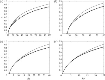
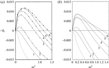
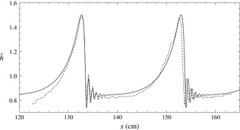
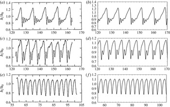
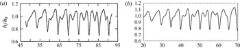
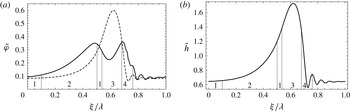
The physical validity of the model has to be tested by comparing its results with the neutral stability curves calculated from the Orr–Sommerfeld equation and with the experimental measurements of travelling waves from Liu & Gollub (Reference Liu and Gollub1994).
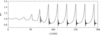
In § 2 we present the long-wave asymptotic expansion. In § 3 we average the mass, momentum and energy equations over the depth and we discuss the structure of the resulting equations. In § 4 we calculate the neutral stability curves. Finally in § 5 we solve numerically the equations of the model and we compare the results with experimental results of Nakoryakov et al. (Reference Nakoryakov, Pokusaev, Alekseenko and Orlov1977), Liu & Gollub (Reference Liu and Gollub1994) and Tihon et al. (Reference Tihon, Serifi, Argyriadi and Bontozoglou2006).
2 Asymptotic expansion
2.1 Nusselt flow
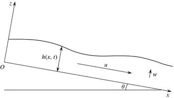
We consider a liquid thin film on an inclined plane. The angle of the plane with respect to the horizontal is
 $\unicode[STIX]{x1D703}$
. The flow is supposed to be two-dimensional. The directions
 $Ox$
and
 $Oz$
are respectively the directions parallel to the plane and normal to the plane. The components of the fluid velocity field are denoted by
 $u$
and
 $w$
in the directions
 $Ox$
and
 $Oz$
respectively. The bottom wall is plane and the fluid depth is denoted by
 $h$
. The notations are specified in figure 1.
Notations used in the text.

The liquid film is thin. If
 $h_{0}$
is the order of magnitude of the fluid depth and
 $L$
the order of magnitude of the typical distance of variations of the variables of the flow in the
 $Ox$
direction, then we can define a small parameter
 $\unicode[STIX]{x1D700}$
by
 $$\begin{eqnarray}\unicode[STIX]{x1D700}=\frac{h_{0}}{L}\ll 1.\end{eqnarray}$$
The liquid is an incompressible Newtonian fluid of density
 $\unicode[STIX]{x1D70C}$
, dynamic viscosity
 $\unicode[STIX]{x1D707}$
and kinematic viscosity
 $\unicode[STIX]{x1D708}=\unicode[STIX]{x1D707}/\unicode[STIX]{x1D70C}$
. Denoting the pressure by
 $p$
, the Cauchy stress tensor
 $\unicode[STIX]{x1D748}$
can be written as
 $\unicode[STIX]{x1D748}=-p\unicode[STIX]{x1D644}+\unicode[STIX]{x1D749}$
where
 $\unicode[STIX]{x1D644}$
is the identity tensor and
 $\unicode[STIX]{x1D749}$
is the viscous stress tensor which is related to the strain rate tensor
 $\unicode[STIX]{x1D63F}$
by
 $\unicode[STIX]{x1D749}=2\unicode[STIX]{x1D707}\unicode[STIX]{x1D63F}$
.
The boundary conditions are the no-penetration condition and the no-slip condition on the bottom and, at the free surface, the kinematic boundary condition and the dynamic boundary condition
 $$\begin{eqnarray}(\unicode[STIX]{x1D748}\,\boldsymbol{n})(z=h)=\frac{\unicode[STIX]{x1D6FE}}{R}\boldsymbol{n},\end{eqnarray}$$
where
 $\unicode[STIX]{x1D6FE}$
is the surface-tension coefficient,
 $R$
the radius of curvature of the free surface and
 $\boldsymbol{n}$
the unit normal vector at the free surface that points towards the atmosphere. The atmospheric pressure is constant and can be taken equal to zero and does not appear in the equations. With the boundary conditions, the Navier–Stokes equations admits a stationary solution with a constant depth
 $h_{0}$
, a parabolic velocity profile
 $$\begin{eqnarray}u(z)=\frac{g\sin \unicode[STIX]{x1D703}}{\unicode[STIX]{x1D708}}z\left(h_{0}-\frac{z}{2}\right),\end{eqnarray}$$
and a hydrostatic pressure distribution
 $$\begin{eqnarray}p(z)=\unicode[STIX]{x1D70C}g(h_{0}-z)\cos \unicode[STIX]{x1D703}.\end{eqnarray}$$
This solution is the Nusselt flow. The velocity averaged over the fluid depth is
 $$\begin{eqnarray}\langle u_{0}\rangle =\frac{gh_{0}^{2}\sin \unicode[STIX]{x1D703}}{3\unicode[STIX]{x1D708}}.\end{eqnarray}$$
The following relation is satisfied for the Nusselt flow:
 $$\begin{eqnarray}\unicode[STIX]{x1D70F}_{xz}(z=0)=\frac{3\unicode[STIX]{x1D707}\langle u_{0}\rangle }{h_{0}}.\end{eqnarray}$$
In order to study a change of Galilean reference frame, we can consider the more general case where the bottom wall has a velocity
 $v_{b}$
in the
 $Ox$
direction. The no-slip condition is then
 $$\begin{eqnarray}u(z=0)=v_{b}.\end{eqnarray}$$
The pressure distribution (2.4) is unchanged and the parabolic velocity profile becomes
 $$\begin{eqnarray}u(z)=\frac{g\sin \unicode[STIX]{x1D703}}{\unicode[STIX]{x1D708}}z\left(h_{0}-\frac{z}{2}\right)+v_{b}.\end{eqnarray}$$
The Galilean invariance is studied in § 3.5. Otherwise, we suppose
 $v_{b}=0$
.
In the following, we consider Nusselt flow as the reference flow which is perturbed when this flow becomes unstable. We perform an asymptotic analysis of this flow in the long-wave regime.
2.2 Dimensionless form of the equations
The equations are put into dimensionless form using the depth
 $h_{0}$
and velocity
 $\langle u_{0}\rangle$
of the Nusselt flow as the characteristic length in the
 $Oz$
direction and characteristic speed in the
 $Ox$
direction. The characteristic length in the
 $Ox$
direction is
 $L=H/\unicode[STIX]{x1D700}$
and the characteristic speed in the
 $Oz$
direction is
 $\unicode[STIX]{x1D700}\langle u_{0}\rangle$
. The following dimensionless numbers can be defined, the Reynolds number
 $$\begin{eqnarray}Re=\frac{h_{0}\langle u_{0}\rangle }{\unicode[STIX]{x1D708}},\end{eqnarray}$$
the Froude number
 $$\begin{eqnarray}F=\frac{\langle u_{0}\rangle }{\sqrt{gh_{0}}}\end{eqnarray}$$
and the Weber number
 $$\begin{eqnarray}We=\frac{\unicode[STIX]{x1D70C}h_{0}\langle u_{0}\rangle ^{2}}{\unicode[STIX]{x1D6FE}}.\end{eqnarray}$$
It follows from equation (2.5) that the dimensionless number defined by
 $\unicode[STIX]{x1D706}=(Re\sin \unicode[STIX]{x1D703})/F^{2}$
satisfies the relation
 $$\begin{eqnarray}\unicode[STIX]{x1D706}=\frac{Re\sin \unicode[STIX]{x1D703}}{F^{2}}=3.\end{eqnarray}$$
Since
 $\unicode[STIX]{x1D706}$
could be different from 3 if a different characteristic speed was used instead of (2.5) to put the equations into dimensionless form, we keep
 $\unicode[STIX]{x1D706}$
in the following equations choosing not to replace it by 3. The following dimensionless quantities, denoted by a tilde, are defined with the scaling of the Nusselt flow and the small parameter
 $\unicode[STIX]{x1D700}$
defined in (2.1) which gives the ratio of transverse to longitudinal spatial scales:
 $$\begin{eqnarray}\left.\begin{array}{@{}l@{}}\tilde{u} ={\displaystyle \frac{u}{\langle u_{0}\rangle }};\quad \tilde{w}={\displaystyle \frac{w}{\unicode[STIX]{x1D700}\langle u_{0}\rangle }};\quad \tilde{x}={\displaystyle \frac{x}{L}};\quad \tilde{z}={\displaystyle \frac{z}{h_{0}}};\quad \tilde{t}={\displaystyle \frac{t}{L}}\langle u_{0}\rangle ;\quad \tilde{h}={\displaystyle \frac{h}{h_{0}}};\\ \tilde{p}={\displaystyle \frac{p}{\unicode[STIX]{x1D70C}gh_{0}}};\quad \tilde{\unicode[STIX]{x1D70F}}_{xx}={\displaystyle \frac{L\unicode[STIX]{x1D70F}_{xx}}{\langle u_{0}\rangle \unicode[STIX]{x1D707}}};\quad \tilde{\unicode[STIX]{x1D70F}}_{zz}={\displaystyle \frac{h_{0}\unicode[STIX]{x1D70F}_{zz}}{\unicode[STIX]{x1D700}\langle u_{0}\rangle \unicode[STIX]{x1D707}}};\quad \tilde{\unicode[STIX]{x1D70F}}_{xz}={\displaystyle \frac{h_{0}\unicode[STIX]{x1D70F}_{xz}}{\langle u_{0}\rangle \unicode[STIX]{x1D707}}}.\end{array}\right\}\end{eqnarray}$$
For convenience, we define the following dimensionless number
 $$\begin{eqnarray}\unicode[STIX]{x1D705}=\frac{\unicode[STIX]{x1D700}^{2}F^{2}}{We}.\end{eqnarray}$$
This number is related to the Eötvös number (also called the Bond number) defined as
 $Eo=Bo=\unicode[STIX]{x0394}\unicode[STIX]{x1D70C}gL^{2}/\unicode[STIX]{x1D6FE}$
(with
 $\unicode[STIX]{x0394}\unicode[STIX]{x1D70C}=\unicode[STIX]{x1D70C}_{liq}-\unicode[STIX]{x1D70C}_{gas}\simeq \unicode[STIX]{x1D70C}$
) by
 $\unicode[STIX]{x1D705}=\unicode[STIX]{x1D700}^{2}/Eo$
. The equations are then put in dimensionless form
 $$\begin{eqnarray}\displaystyle & \displaystyle \frac{\unicode[STIX]{x2202}\tilde{u} }{\unicode[STIX]{x2202}\tilde{x}}+\frac{\unicode[STIX]{x2202}\tilde{w}}{\unicode[STIX]{x2202}\tilde{z}}=0, & \displaystyle\end{eqnarray}$$
 $$\begin{eqnarray}\displaystyle & \displaystyle \frac{\unicode[STIX]{x2202}\tilde{u} }{\unicode[STIX]{x2202}\tilde{t}}+\frac{\unicode[STIX]{x2202}\tilde{u} ^{2}}{\unicode[STIX]{x2202}\tilde{x}}+\frac{\unicode[STIX]{x2202}\tilde{u} \tilde{w}}{\unicode[STIX]{x2202}\tilde{z}}=\frac{\unicode[STIX]{x1D706}}{\unicode[STIX]{x1D700}Re}-\frac{1}{F^{2}}\frac{\unicode[STIX]{x2202}\tilde{p}}{\unicode[STIX]{x2202}\tilde{x}}+\frac{\unicode[STIX]{x1D700}}{Re}\frac{\unicode[STIX]{x2202}\tilde{\unicode[STIX]{x1D70F}}_{xx}}{\unicode[STIX]{x2202}\tilde{x}}+\frac{1}{\unicode[STIX]{x1D700}Re}\frac{\unicode[STIX]{x2202}\tilde{\unicode[STIX]{x1D70F}}_{xz}}{\unicode[STIX]{x2202}\tilde{z}}, & \displaystyle\end{eqnarray}$$
 $$\begin{eqnarray}\displaystyle & \displaystyle \unicode[STIX]{x1D700}^{2}F^{2}\left(\frac{\unicode[STIX]{x2202}\tilde{w}}{\unicode[STIX]{x2202}\tilde{t}}+\frac{\unicode[STIX]{x2202}\tilde{u} \tilde{w}}{\unicode[STIX]{x2202}\tilde{x}}+\frac{\unicode[STIX]{x2202}\tilde{w}^{2}}{\unicode[STIX]{x2202}\tilde{z}}\right)=-\cos \unicode[STIX]{x1D703}-\frac{\unicode[STIX]{x2202}\tilde{p}}{\unicode[STIX]{x2202}\tilde{z}}+\frac{\unicode[STIX]{x1D700}F^{2}}{Re}\frac{\unicode[STIX]{x2202}\tilde{\unicode[STIX]{x1D70F}}_{zz}}{\unicode[STIX]{x2202}\tilde{z}}+\frac{\unicode[STIX]{x1D700}F^{2}}{Re}\frac{\unicode[STIX]{x2202}\tilde{\unicode[STIX]{x1D70F}}_{xz}}{\unicode[STIX]{x2202}\tilde{x}}, & \displaystyle\end{eqnarray}$$
 $$\begin{eqnarray}\tilde{\unicode[STIX]{x1D70F}}_{xz}=\frac{\unicode[STIX]{x2202}\tilde{u} }{\unicode[STIX]{x2202}\tilde{z}}+\unicode[STIX]{x1D700}^{2}\frac{\unicode[STIX]{x2202}\tilde{w}}{\unicode[STIX]{x2202}\tilde{x}};\quad \tilde{\unicode[STIX]{x1D70F}}_{xx}=-\tilde{\unicode[STIX]{x1D70F}}_{zz}=2\frac{\unicode[STIX]{x2202}\tilde{u} }{\unicode[STIX]{x2202}\tilde{x}},\end{eqnarray}$$
 $$\begin{eqnarray}\tilde{w}(\tilde{z}=0)=0;\quad \tilde{u} (\tilde{z}=0)=0;\end{eqnarray}$$
 $$\begin{eqnarray}\frac{\unicode[STIX]{x2202}\tilde{h}}{\unicode[STIX]{x2202}\tilde{t}}+\tilde{u} (\tilde{h})\frac{\unicode[STIX]{x2202}\tilde{h}}{\unicode[STIX]{x2202}\tilde{x}}=\tilde{w}(\tilde{h}),\end{eqnarray}$$
 $$\begin{eqnarray}\tilde{\unicode[STIX]{x1D70F}}_{xz}(\tilde{h})+\left[\frac{\unicode[STIX]{x1D700}Re}{F^{2}}\tilde{p}(\tilde{h})-\unicode[STIX]{x1D700}^{2}\tilde{\unicode[STIX]{x1D70F}}_{xx}(\tilde{h})\right]\frac{\unicode[STIX]{x2202}\tilde{h}}{\unicode[STIX]{x2202}\tilde{x}}+\unicode[STIX]{x1D705}\frac{\unicode[STIX]{x1D700}Re}{F^{2}}\frac{\unicode[STIX]{x2202}\tilde{h}}{\unicode[STIX]{x2202}\tilde{x}}\frac{\unicode[STIX]{x2202}^{2}\tilde{h}}{\unicode[STIX]{x2202}\tilde{x}^{2}}\left[1+\unicode[STIX]{x1D700}^{2}\left(\frac{\unicode[STIX]{x2202}\tilde{h}}{\unicode[STIX]{x2202}\tilde{x}}\right)^{2}\right]^{-3/2}=0\end{eqnarray}$$
 $$\begin{eqnarray}\tilde{p}(\tilde{h})+\frac{\unicode[STIX]{x1D700}F^{2}}{Re}\frac{\unicode[STIX]{x2202}\tilde{h}}{\unicode[STIX]{x2202}\tilde{x}}\tilde{\unicode[STIX]{x1D70F}}_{xz}(\tilde{h})-\frac{\unicode[STIX]{x1D700}F^{2}}{Re}\tilde{\unicode[STIX]{x1D70F}}_{zz}(\tilde{h})+\unicode[STIX]{x1D705}\frac{\unicode[STIX]{x2202}^{2}\tilde{h}}{\unicode[STIX]{x2202}\tilde{x}^{2}}\left[1+\unicode[STIX]{x1D700}^{2}\left(\frac{\unicode[STIX]{x2202}\tilde{h}}{\unicode[STIX]{x2202}\tilde{x}}\right)^{2}\right]^{-3/2}=0.\end{eqnarray}$$
Equation (2.15) is the dimensionless continuity equation. Equations (2.16)–(2.17) are the Navier–Stokes momentum equations. Equation (2.18) gives the relation between the components of the viscous stress tensor and those of the strain rate tensor and equations (2.19)–(2.22) are the dimensionless boundary conditions.
2.3 Successive approximations
2.3.1 Approximations up to first order
The variables of equations (2.15)–(2.22) are expanded in formal power series of
 $\unicode[STIX]{x1D700}$
:
 $$\begin{eqnarray}\tilde{u} =\tilde{u} _{0}+\unicode[STIX]{x1D700}\tilde{u} _{1}+\unicode[STIX]{x1D700}^{2}\tilde{u} _{2}+\cdots\end{eqnarray}$$
 $$\begin{eqnarray}\tilde{w}=\tilde{w}_{0}+\unicode[STIX]{x1D700}\tilde{w}_{1}+\unicode[STIX]{x1D700}^{2}\tilde{w}_{2}+\cdots\end{eqnarray}$$
 $$\begin{eqnarray}\tilde{p}=\tilde{p}_{0}+\unicode[STIX]{x1D700}\tilde{p}_{1}+\unicode[STIX]{x1D700}^{2}\tilde{p}_{2}+\cdots\end{eqnarray}$$
 $$\begin{eqnarray}\tilde{\unicode[STIX]{x1D70F}}_{xz}=\tilde{\unicode[STIX]{x1D70F}}_{0}+\unicode[STIX]{x1D700}\tilde{\unicode[STIX]{x1D70F}}_{1}+\unicode[STIX]{x1D700}^{2}\tilde{\unicode[STIX]{x1D70F}}_{2}+\cdots \,.\end{eqnarray}$$
The Reynolds number
 $Re$
, the angle
 $\unicode[STIX]{x1D703}$
and
 $\unicode[STIX]{x1D705}$
are supposed to be of
 $O(1)$
. The solution of order 0 is:
 $$\begin{eqnarray}\tilde{\unicode[STIX]{x1D70F}}_{0}=\unicode[STIX]{x1D706}(\tilde{h}-\tilde{z})\end{eqnarray}$$
 $$\begin{eqnarray}\tilde{u} _{0}=\unicode[STIX]{x1D706}\tilde{z}\left(\tilde{h}-\frac{\tilde{z}}{2}\right)\end{eqnarray}$$
 $$\begin{eqnarray}\tilde{w}_{0}=-\frac{\unicode[STIX]{x1D706}}{2}\tilde{z}^{2}\frac{\unicode[STIX]{x2202}\tilde{h}}{\unicode[STIX]{x2202}\tilde{x}}\end{eqnarray}$$
 $$\begin{eqnarray}\tilde{p}_{0}=(\tilde{h}-\tilde{z})\cos \unicode[STIX]{x1D703}-\unicode[STIX]{x1D705}\frac{\unicode[STIX]{x2202}^{2}\tilde{h}}{\unicode[STIX]{x2202}\tilde{x}^{2}}.\end{eqnarray}$$
Equation (2.28) shows that at order 0, the parabolic profile is recovered. The velocity
 $\tilde{u} _{0}$
averaged over the fluid depth, written
 $\langle \tilde{u} _{0}\rangle$
, is
 $$\begin{eqnarray}\langle \tilde{u} _{0}\rangle =\frac{\unicode[STIX]{x1D706}\tilde{h}^{2}}{3}.\end{eqnarray}$$
At order 0, the expression of
 $\tilde{\unicode[STIX]{x1D70F}}_{xz}$
at
 $z=0$
is
 $$\begin{eqnarray}\tilde{\unicode[STIX]{x1D70F}}_{0}(0)=\frac{3\langle \tilde{u} _{0}\rangle }{\tilde{h}}.\end{eqnarray}$$
With the solutions of order 0 (2.27)–(2.30), solutions of order 1 can be found. The important results are the expression of
 $\tilde{\unicode[STIX]{x1D70F}}_{1}$
at
 $z=0$
 $$\begin{eqnarray}\frac{\tilde{\unicode[STIX]{x1D70F}}_{1}(0)}{Re}=\left(\frac{1}{3}\unicode[STIX]{x1D706}^{2}\tilde{h}^{3}-\frac{\cos \unicode[STIX]{x1D703}}{F^{2}}\right)\tilde{h}\frac{\unicode[STIX]{x2202}\tilde{h}}{\unicode[STIX]{x2202}\tilde{x}}+\frac{\unicode[STIX]{x1D705}}{F^{2}}\tilde{h}\frac{\unicode[STIX]{x2202}^{3}\tilde{h}}{\unicode[STIX]{x2202}\tilde{x}^{3}}\end{eqnarray}$$
and the expression of
 $\tilde{u} _{1}$
averaged over the depth, denoted by
 $\langle \tilde{u} _{1}\rangle$
,
 $$\begin{eqnarray}\frac{3\langle \tilde{u} _{1}\rangle }{Re\;\tilde{h}}=\left(\frac{2}{5}\unicode[STIX]{x1D706}^{2}\tilde{h}^{3}-\frac{\cos \unicode[STIX]{x1D703}}{F^{2}}\right)\tilde{h}\frac{\unicode[STIX]{x2202}\tilde{h}}{\unicode[STIX]{x2202}\tilde{x}}+\frac{\unicode[STIX]{x1D705}}{F^{2}}\tilde{h}\frac{\unicode[STIX]{x2202}^{3}\tilde{h}}{\unicode[STIX]{x2202}\tilde{x}^{3}}.\end{eqnarray}$$
At order 1, it can be seen that
 $$\begin{eqnarray}\tilde{\unicode[STIX]{x1D70F}}_{1}(0)\neq \frac{3\langle \tilde{u} _{1}\rangle }{\tilde{h}}.\end{eqnarray}$$
2.3.2 Approximations up to second order
While it is perfectly possible to get a fully consistent asymptotic expansion to the second order, it appears that many of these terms not only are very complicated and give an unsatisfactory structure to the equations but also they are not essential. The main results of the full second-order expansion are given in appendix A. The complete explanations can be found in Noble & Vila (Reference Noble and Vila2013).
From this point onward, we apply the following principle: for each physical effect, we keep only the non-vanishing terms of the highest order of magnitude, i.e. the leading-order terms. This principle is first applied to the surface-tension effects. To avoid unnecessary capillary terms of lower order of magnitude in the second-order asymptotic expansion, the dimensionless number
 $\unicode[STIX]{x1D705}$
is now supposed to be
 $O(\unicode[STIX]{x1D700})$
. We introduce
 $\unicode[STIX]{x1D705}_{1}$
as
 $$\begin{eqnarray}\unicode[STIX]{x1D705}=\unicode[STIX]{x1D700}\unicode[STIX]{x1D705}_{1},\end{eqnarray}$$
with
 $\unicode[STIX]{x1D705}_{1}=O(1)$
. At the first order of approximation, every physical effects can be included, except diffusion. The second-order terms are important mainly because they allow us to include the viscous diffusion that the first-order model is lacking. All other second-order terms are not necessary since the physical effects are already included at the first order. Consequently, only viscous diffusive and capillary dispersive terms will be kept in the second-order expansion. Note that a viscous diffusive term is quasi-linear and of
 $O(\unicode[STIX]{x1D700}/Re)$
.
The expansions of order 1 are modified as follows:
 $$\begin{eqnarray}\frac{\tilde{\unicode[STIX]{x1D70F}}_{1}(0)}{Re}=\left(\frac{1}{3}\unicode[STIX]{x1D706}^{2}\tilde{h}^{3}-\frac{\cos \unicode[STIX]{x1D703}}{F^{2}}\right)\tilde{h}\frac{\unicode[STIX]{x2202}\tilde{h}}{\unicode[STIX]{x2202}\tilde{x}}\end{eqnarray}$$
 $$\begin{eqnarray}\frac{3\langle \tilde{u} _{1}\rangle }{Re\;\tilde{h}}=\left(\frac{2}{5}\unicode[STIX]{x1D706}^{2}\tilde{h}^{3}-\frac{\cos \unicode[STIX]{x1D703}}{F^{2}}\right)\tilde{h}\frac{\unicode[STIX]{x2202}\tilde{h}}{\unicode[STIX]{x2202}\tilde{x}}.\end{eqnarray}$$
Keeping only viscous diffusive and capillary terms, we get the following expressions of order 2:
 $$\begin{eqnarray}\tilde{\unicode[STIX]{x1D70F}}_{2}(0)=\frac{5}{2}\unicode[STIX]{x1D706}\tilde{h}^{2}\frac{\unicode[STIX]{x2202}^{2}\tilde{h}}{\unicode[STIX]{x2202}\tilde{x}^{2}}+Re\frac{\unicode[STIX]{x1D705}_{1}}{F^{2}}\tilde{h}\frac{\unicode[STIX]{x2202}^{3}\tilde{h}}{\unicode[STIX]{x2202}\tilde{x}^{3}}\end{eqnarray}$$
and
 $$\begin{eqnarray}\frac{3\langle \tilde{u} _{2}\rangle }{\tilde{h}}=3\unicode[STIX]{x1D706}\tilde{h}^{2}\frac{\unicode[STIX]{x2202}^{2}\tilde{h}}{\unicode[STIX]{x2202}\tilde{x}^{2}}+Re\frac{\unicode[STIX]{x1D705}_{1}}{F^{2}}\tilde{h}\frac{\unicode[STIX]{x2202}^{3}\tilde{h}}{\unicode[STIX]{x2202}\tilde{x}^{3}}.\end{eqnarray}$$
3 Averaged equations
The equations (2.15)–(2.16) are averaged over the depth. For any variable
 $A$
of the flow, the averaged value of
 $A$
, denoted by
 $\langle A\rangle$
, is defined by
 $$\begin{eqnarray}\langle A\rangle =\frac{1}{h}\int _{0}^{h}A~\text{d}z.\end{eqnarray}$$
For the velocity, we use the special notation
 $\langle u\rangle =U$
.
3.1 Mass conservation
The mass equation (2.15) is averaged over the depth. With the kinematic boundary condition (2.20), we get the exact equation
 $$\begin{eqnarray}\frac{\unicode[STIX]{x2202}\tilde{h}}{\unicode[STIX]{x2202}\tilde{t}}+\frac{\unicode[STIX]{x2202}\tilde{h}\tilde{U} }{\unicode[STIX]{x2202}\tilde{x}}=0.\end{eqnarray}$$
If the asymptotic solution of order 0 for
 $\tilde{U}$
is used, i.e. if
 $\tilde{U} =\langle \tilde{u} _{0}\rangle$
, then equation (3.2) together with the expression (2.31) of
 $\langle \tilde{u} _{0}\rangle$
gives the kinematic wave equation
 $$\begin{eqnarray}\frac{\unicode[STIX]{x2202}\tilde{h}}{\unicode[STIX]{x2202}\tilde{t}}+\unicode[STIX]{x1D706}\tilde{h}^{2}\frac{\unicode[STIX]{x2202}\tilde{h}}{\unicode[STIX]{x2202}\tilde{x}}=O(\unicode[STIX]{x1D700}),\end{eqnarray}$$
which shows that a depth perturbation is propagated at the celerity
 $\tilde{c}_{0}=\unicode[STIX]{x1D706}\tilde{h}^{2}$
which is equal to
 $3\tilde{U}$
. This is the celerity of the kinematic waves.
3.2 Momentum balance
The momentum balance equation (2.16) is averaged over the depth. Using the no-penetration condition (2.19), the kinematic boundary condition (2.20) and the dynamic boundary conditions (2.21) and (2.22) written
 $$\begin{eqnarray}\tilde{\unicode[STIX]{x1D70F}}_{xz}(\tilde{h})+\left[\frac{\unicode[STIX]{x1D700}Re}{F^{2}}\tilde{p}(\tilde{h})-\unicode[STIX]{x1D700}^{2}\tilde{\unicode[STIX]{x1D70F}}_{xx}(\tilde{h})\right]\frac{\unicode[STIX]{x2202}\tilde{h}}{\unicode[STIX]{x2202}\tilde{x}}+\unicode[STIX]{x1D705}_{1}\frac{\unicode[STIX]{x1D700}^{2}Re}{F^{2}}\frac{\unicode[STIX]{x2202}\tilde{h}}{\unicode[STIX]{x2202}\tilde{x}}\frac{\unicode[STIX]{x2202}^{2}\tilde{h}}{\unicode[STIX]{x2202}\tilde{x}^{2}}=0\end{eqnarray}$$
 $$\begin{eqnarray}\tilde{p}(\tilde{h})+\frac{\unicode[STIX]{x1D700}F^{2}}{Re}\frac{\unicode[STIX]{x2202}\tilde{h}}{\unicode[STIX]{x2202}\tilde{x}}\tilde{\unicode[STIX]{x1D70F}}_{xz}(\tilde{h})-\frac{\unicode[STIX]{x1D700}F^{2}}{Re}\tilde{\unicode[STIX]{x1D70F}}_{zz}(\tilde{h})+\unicode[STIX]{x1D700}\unicode[STIX]{x1D705}_{1}\frac{\unicode[STIX]{x2202}^{2}\tilde{h}}{\unicode[STIX]{x2202}\tilde{x}^{2}}=0,\end{eqnarray}$$
the following equation is found
 $$\begin{eqnarray}\displaystyle & & \displaystyle \frac{\unicode[STIX]{x2202}\tilde{h}\tilde{U} }{\unicode[STIX]{x2202}\tilde{t}}+\frac{\unicode[STIX]{x2202}}{\unicode[STIX]{x2202}\tilde{x}}\left(\tilde{h}\langle \tilde{u} ^{2}\rangle +\frac{1}{F^{2}}\int _{0}^{\tilde{h}}\tilde{p}\;\text{d}\tilde{z}-\frac{\unicode[STIX]{x1D700}}{Re}\int _{0}^{\tilde{h}}\tilde{\unicode[STIX]{x1D70F}}_{xx}\;\text{d}\tilde{z}\right)\nonumber\\ \displaystyle & & \displaystyle \quad =\frac{\unicode[STIX]{x1D706}\tilde{h}-\tilde{\unicode[STIX]{x1D70F}}_{xz}(0)}{\unicode[STIX]{x1D700}Re}-\unicode[STIX]{x1D700}\frac{\unicode[STIX]{x1D705}_{1}}{F^{2}}\frac{\unicode[STIX]{x2202}\tilde{h}}{\unicode[STIX]{x2202}\tilde{x}}\frac{\unicode[STIX]{x2202}^{2}\tilde{h}}{\unicode[STIX]{x2202}\tilde{x}^{2}}+O(\unicode[STIX]{x1D700}).\end{eqnarray}$$
Equation (2.17) is used to express the integral of the pressure of (3.6). The left-hand side of (2.17) is of
 $O(\unicode[STIX]{x1D700}^{2})$
and hence it does not appear in the second-order model. The integration of (2.17) with the boundary conditions leads to
 $$\begin{eqnarray}\tilde{p}(\tilde{z})=(\tilde{h}-\tilde{z})\cos \unicode[STIX]{x1D703}-\unicode[STIX]{x1D700}\unicode[STIX]{x1D705}_{1}\frac{\unicode[STIX]{x2202}^{2}\tilde{h}}{\unicode[STIX]{x2202}\tilde{x}^{2}}+\frac{\unicode[STIX]{x1D700}F^{2}}{Re}\tilde{\unicode[STIX]{x1D70F}}_{zz}(\tilde{z})+\frac{\unicode[STIX]{x1D700}F^{2}}{Re}\frac{\unicode[STIX]{x2202}}{\unicode[STIX]{x2202}\tilde{x}}\int _{\tilde{h}}^{\tilde{z}}\tilde{\unicode[STIX]{x1D70F}}_{xz}\,\text{d}\tilde{z}.\end{eqnarray}$$
With this expression of the pressure, and since (2.18) implies that
 $\tilde{\unicode[STIX]{x1D70F}}_{zz}=-\tilde{\unicode[STIX]{x1D70F}}_{xx}$
, equation (3.6) becomes
 $$\begin{eqnarray}\displaystyle & & \displaystyle \frac{\unicode[STIX]{x2202}\tilde{h}\tilde{U} }{\unicode[STIX]{x2202}\tilde{t}}+\frac{\unicode[STIX]{x2202}}{\unicode[STIX]{x2202}\tilde{x}}\left(\tilde{h}\langle \tilde{u} ^{2}\rangle +\frac{\tilde{h}^{2}\cos \unicode[STIX]{x1D703}}{2F^{2}}+\frac{\unicode[STIX]{x1D700}}{Re}\int _{0}^{\tilde{h}}\text{d}\tilde{z}\frac{\unicode[STIX]{x2202}}{\unicode[STIX]{x2202}\tilde{x}}\int _{\tilde{h}}^{\tilde{z}}\tilde{\unicode[STIX]{x1D70F}}_{xz}\;\text{d}\tilde{z}-2\frac{\unicode[STIX]{x1D700}}{Re}\int _{0}^{\tilde{h}}\tilde{\unicode[STIX]{x1D70F}}_{xx}\;\text{d}\tilde{z}\right)\nonumber\\ \displaystyle & & \displaystyle \quad =\frac{\unicode[STIX]{x1D706}\tilde{h}-\tilde{\unicode[STIX]{x1D70F}}_{xz}(0)}{\unicode[STIX]{x1D700}Re}+\unicode[STIX]{x1D700}\frac{\unicode[STIX]{x1D705}_{1}}{F^{2}}\tilde{h}\frac{\unicode[STIX]{x2202}^{3}\tilde{h}}{\unicode[STIX]{x2202}\tilde{x}^{3}}.\end{eqnarray}$$
The two terms with integrals can be calculated with the expressions of the components of the viscous stress tensor given by (2.18) with
 $\tilde{\unicode[STIX]{x1D70F}}_{xz}=\unicode[STIX]{x2202}\tilde{u} /\unicode[STIX]{x2202}\tilde{z}+O(\unicode[STIX]{x1D700}^{2})$
. The result depends on the value of
 $\tilde{u}$
at
 $\tilde{z}=\tilde{h}$
, denoted by
 $\tilde{u} (\tilde{h})$
:
 $$\begin{eqnarray}\displaystyle & & \displaystyle \frac{\unicode[STIX]{x2202}\tilde{h}\tilde{U} }{\unicode[STIX]{x2202}\tilde{t}}+\frac{\unicode[STIX]{x2202}}{\unicode[STIX]{x2202}\tilde{x}}\left(\tilde{h}\langle \tilde{u} ^{2}\rangle +\frac{\tilde{h}^{2}\cos \unicode[STIX]{x1D703}}{2F^{2}}-3\frac{\unicode[STIX]{x1D700}}{Re}\frac{\unicode[STIX]{x2202}\tilde{h}\tilde{U} }{\unicode[STIX]{x2202}\tilde{x}}+3\frac{\unicode[STIX]{x1D700}}{Re}\tilde{u} (\tilde{h})\frac{\unicode[STIX]{x2202}\tilde{h}}{\unicode[STIX]{x2202}\tilde{x}}-\frac{\unicode[STIX]{x1D700}}{Re}\tilde{h}\frac{\unicode[STIX]{x2202}\tilde{u} (\tilde{h})}{\unicode[STIX]{x2202}\tilde{x}}\right)\nonumber\\ \displaystyle & & \displaystyle \quad =\frac{\unicode[STIX]{x1D706}\tilde{h}-\tilde{\unicode[STIX]{x1D70F}}_{xz}(0)}{\unicode[STIX]{x1D700}Re}+\unicode[STIX]{x1D700}\frac{\unicode[STIX]{x1D705}_{1}}{F^{2}}\tilde{h}\frac{\unicode[STIX]{x2202}^{3}\tilde{h}}{\unicode[STIX]{x2202}\tilde{x}^{3}}.\end{eqnarray}$$
Since the terms involving
 $\tilde{u} (\tilde{h})$
are all of second order,
 $\tilde{u} (\tilde{h})$
can be evaluated at order 0. As
 $\tilde{u} _{0}(\tilde{h})=\unicode[STIX]{x1D706}\tilde{h}^{2}/2$
and
 $\langle \tilde{u} _{0}\rangle =\unicode[STIX]{x1D706}\tilde{h}^{2}/3$
(see (2.28) and (2.31)),
 $$\begin{eqnarray}\tilde{u} (\tilde{h})={\textstyle \frac{3}{2}}\tilde{U} +O(\unicode[STIX]{x1D700}).\end{eqnarray}$$
Equation (3.9) becomes
 $$\begin{eqnarray}\displaystyle & & \displaystyle \frac{\unicode[STIX]{x2202}\tilde{h}\tilde{U} }{\unicode[STIX]{x2202}\tilde{t}}+\frac{\unicode[STIX]{x2202}}{\unicode[STIX]{x2202}\tilde{x}}\left(\tilde{h}\langle \tilde{u} ^{2}\rangle +\frac{\tilde{h}^{2}\cos \unicode[STIX]{x1D703}}{2F^{2}}-\frac{\unicode[STIX]{x1D700}}{Re}\frac{9}{2}\tilde{h}\frac{\unicode[STIX]{x2202}\tilde{U} }{\unicode[STIX]{x2202}\tilde{x}}+\frac{\unicode[STIX]{x1D700}}{Re}\frac{3}{2}\tilde{U} \frac{\unicode[STIX]{x2202}\tilde{h}}{\unicode[STIX]{x2202}\tilde{x}}\right)\nonumber\\ \displaystyle & & \displaystyle \quad =\frac{\unicode[STIX]{x1D706}\tilde{h}-\tilde{\unicode[STIX]{x1D70F}}_{xz}(0)}{\unicode[STIX]{x1D700}Re}+\unicode[STIX]{x1D700}\frac{\unicode[STIX]{x1D705}_{1}}{F^{2}}\tilde{h}\frac{\unicode[STIX]{x2202}^{3}\tilde{h}}{\unicode[STIX]{x2202}\tilde{x}^{3}}.\end{eqnarray}$$
The two terms of
 $O(\unicode[STIX]{x1D700}/Re)$
can be estimated at order 0:
 $$\begin{eqnarray}\frac{\unicode[STIX]{x1D700}}{Re}\left(-\frac{9}{2}\tilde{h}\frac{\unicode[STIX]{x2202}\tilde{U} }{\unicode[STIX]{x2202}\tilde{x}}+\frac{3}{2}\tilde{U} \frac{\unicode[STIX]{x2202}\tilde{h}}{\unicode[STIX]{x2202}\tilde{x}}\right)=-\frac{\unicode[STIX]{x1D700}}{Re}\frac{15}{4}\tilde{h}\frac{\unicode[STIX]{x2202}\tilde{U} }{\unicode[STIX]{x2202}\tilde{x}}+O(\unicode[STIX]{x1D700}^{2}).\end{eqnarray}$$
Written this way, this term has the form of a viscous diffusive term. Equation (3.11) can therefore be written
 $$\begin{eqnarray}\displaystyle & & \displaystyle \frac{\unicode[STIX]{x2202}\tilde{h}\tilde{U} }{\unicode[STIX]{x2202}\tilde{t}}+\frac{\unicode[STIX]{x2202}}{\unicode[STIX]{x2202}\tilde{x}}\left(\tilde{h}\langle \tilde{u} ^{2}\rangle +\frac{\tilde{h}^{2}\cos \unicode[STIX]{x1D703}}{2F^{2}}\right)\nonumber\\ \displaystyle & & \displaystyle \quad =\frac{\unicode[STIX]{x1D706}\tilde{h}-\tilde{\unicode[STIX]{x1D70F}}_{xz}(0)}{\unicode[STIX]{x1D700}Re}+\frac{\unicode[STIX]{x1D700}}{Re}\frac{\unicode[STIX]{x2202}}{\unicode[STIX]{x2202}\tilde{x}}\left(\frac{15}{4}\tilde{h}\frac{\unicode[STIX]{x2202}\tilde{U} }{\unicode[STIX]{x2202}\tilde{x}}\right)+\unicode[STIX]{x1D700}\frac{\unicode[STIX]{x1D705}_{1}}{F^{2}}\tilde{h}\frac{\unicode[STIX]{x2202}^{3}\tilde{h}}{\unicode[STIX]{x2202}\tilde{x}^{3}}.\end{eqnarray}$$
To write this equation at the first order of approximation, the order of magnitude of
 $\unicode[STIX]{x1D705}$
has to be increased to
 $O(1)$
(i.e.
 $\unicode[STIX]{x1D700}\unicode[STIX]{x1D705}_{1}$
is replaced by
 $\unicode[STIX]{x1D705}$
). The averaged momentum equation reduces to
 $$\begin{eqnarray}\frac{\unicode[STIX]{x2202}\tilde{h}\tilde{U} }{\unicode[STIX]{x2202}\tilde{t}}+\frac{\unicode[STIX]{x2202}}{\unicode[STIX]{x2202}\tilde{x}}\left(\tilde{h}\langle \tilde{u} ^{2}\rangle +\frac{\tilde{h}^{2}\cos \unicode[STIX]{x1D703}}{2F^{2}}\right)=\frac{\unicode[STIX]{x1D706}\tilde{h}-\tilde{\unicode[STIX]{x1D70F}}_{xz}(0)}{\unicode[STIX]{x1D700}Re}+\frac{\unicode[STIX]{x1D705}}{F^{2}}\tilde{h}\frac{\unicode[STIX]{x2202}^{3}\tilde{h}}{\unicode[STIX]{x2202}\tilde{x}^{3}}.\end{eqnarray}$$
The velocity
 $\tilde{u}$
is decomposed as the sum of its average value
 $\tilde{U}$
and a fluctuation
 $\tilde{u} ^{\prime }$
which depends on
 $\tilde{x}$
,
 $\tilde{z}$
and
 $\tilde{t}$
:
 $$\begin{eqnarray}\tilde{u} (\tilde{x},\tilde{z},\tilde{t})=\tilde{U} (\tilde{x},\tilde{t})+\tilde{u} ^{\prime }(\tilde{x},\tilde{z},\tilde{t}).\end{eqnarray}$$
By definition,
 $\langle \tilde{u} ^{\prime }\rangle =0$
. The quantity
 $\langle \tilde{u} ^{2}\rangle$
can be written
 $$\begin{eqnarray}\langle \tilde{u} ^{2}\rangle =\tilde{U} ^{2}+\langle \tilde{u} ^{\prime 2}\rangle .\end{eqnarray}$$
At the first order of approximation,
 $\langle \tilde{u} ^{\prime 2}\rangle$
could be estimated at order 0 either as a function of
 $\tilde{h}$
 $$\begin{eqnarray}\langle \tilde{u} ^{\prime 2}\rangle =\frac{\unicode[STIX]{x1D706}^{2}\tilde{h}^{4}}{45}+O(\unicode[STIX]{x1D700})\end{eqnarray}$$
or as a function of
 $\tilde{U}$
 $$\begin{eqnarray}\langle \tilde{u} ^{\prime 2}\rangle =\frac{\tilde{U} ^{2}}{5}+O(\unicode[STIX]{x1D700}).\end{eqnarray}$$
In the latter case, the first-order equation (3.14) becomes
 $$\begin{eqnarray}\frac{\unicode[STIX]{x2202}\tilde{h}\tilde{U} }{\unicode[STIX]{x2202}\tilde{t}}+\frac{\unicode[STIX]{x2202}}{\unicode[STIX]{x2202}\tilde{x}}\left(\frac{6}{5}\tilde{h}\tilde{U} ^{2}+\frac{\tilde{h}^{2}\cos \unicode[STIX]{x1D703}}{2F^{2}}\right)=\frac{\unicode[STIX]{x1D706}\tilde{h}-\tilde{\unicode[STIX]{x1D70F}}_{xz}(0)}{\unicode[STIX]{x1D700}Re}+\frac{\unicode[STIX]{x1D705}}{F^{2}}\tilde{h}\frac{\unicode[STIX]{x2202}^{3}\tilde{h}}{\unicode[STIX]{x2202}\tilde{x}^{3}}.\end{eqnarray}$$
If now
 $\tilde{\unicode[STIX]{x1D70F}}_{xz}(0)$
is supposed to be equal to
 $3\tilde{U} /\tilde{h}$
, which is true at order 0 but wrong at order 1 (see (2.35)), equation (3.19) gives the Shkadov equation. The first-order correction to
 $\tilde{\unicode[STIX]{x1D70F}}_{xz}(0)$
cannot be neglected, even at the first order of approximation. Using the asymptotic expansion
 $\tilde{\unicode[STIX]{x1D70F}}_{xz}=\tilde{\unicode[STIX]{x1D70F}}_{0}+\unicode[STIX]{x1D700}\tilde{\unicode[STIX]{x1D70F}}_{1}+\unicode[STIX]{x1D700}^{2}\tilde{\unicode[STIX]{x1D70F}}_{2}+\cdots$
and the expression
 $\tilde{\unicode[STIX]{x1D70F}}_{0}(0)=\unicode[STIX]{x1D706}\tilde{h}$
coming from (2.27), a consistent form of equation (3.19) is
 $$\begin{eqnarray}\frac{\unicode[STIX]{x2202}\tilde{h}\tilde{U} }{\unicode[STIX]{x2202}\tilde{t}}+\frac{\unicode[STIX]{x2202}}{\unicode[STIX]{x2202}\tilde{x}}\left(\frac{6}{5}\tilde{h}\tilde{U} ^{2}+\frac{\tilde{h}^{2}\cos \unicode[STIX]{x1D703}}{2F^{2}}\right)=-\frac{\tilde{\unicode[STIX]{x1D70F}}_{1}(0)}{Re}+\frac{\unicode[STIX]{x1D705}}{F^{2}}\tilde{h}\frac{\unicode[STIX]{x2202}^{3}\tilde{h}}{\unicode[STIX]{x2202}\tilde{x}^{3}}.\end{eqnarray}$$
At the first order,
 $$\begin{eqnarray}\langle \tilde{u} _{1}\rangle =\frac{\tilde{U} -\langle \tilde{u} _{0}\rangle }{\unicode[STIX]{x1D700}}+O(\unicode[STIX]{x1D700}).\end{eqnarray}$$
Since
 $\tilde{\unicode[STIX]{x1D70F}}_{1}(0)\neq 3\langle \tilde{u} _{1}\rangle /\tilde{h}$
,
 $$\begin{eqnarray}-\frac{\tilde{\unicode[STIX]{x1D70F}}_{1}(0)}{Re}\neq \frac{1}{\unicode[STIX]{x1D700}Re}\left(\unicode[STIX]{x1D706}\tilde{h}-\frac{3\tilde{U} }{\tilde{h}}\right).\end{eqnarray}$$
Therefore, the Shkadov equation is not consistent. However it is possible to derive a consistent two-equation model. For instance, the asymptotic expansions (2.33) and (2.34) allow us to write
 $$\begin{eqnarray}\frac{\tilde{\unicode[STIX]{x1D70F}}_{1}(0)}{Re}=\frac{5}{6}\frac{1}{Re}\frac{3\langle \tilde{u} _{1}\rangle }{\;\tilde{h}}-\frac{1}{12}\frac{\cos \unicode[STIX]{x1D703}}{F^{2}}\frac{\unicode[STIX]{x2202}\tilde{h}^{2}}{\unicode[STIX]{x2202}\tilde{x}}+\frac{1}{6}\frac{\unicode[STIX]{x1D705}}{F^{2}}\tilde{h}\frac{\unicode[STIX]{x2202}^{3}\tilde{h}}{\unicode[STIX]{x2202}\tilde{x}^{3}}.\end{eqnarray}$$
Using this expression (3.23) and the expression (3.17), equation (3.14) becomes
 $$\begin{eqnarray}\displaystyle & & \displaystyle \frac{\unicode[STIX]{x2202}\tilde{h}\tilde{U} }{\unicode[STIX]{x2202}\tilde{t}}+\frac{\unicode[STIX]{x2202}}{\unicode[STIX]{x2202}\tilde{x}}\left(\tilde{h}\tilde{U} ^{2}+\frac{\unicode[STIX]{x1D706}^{2}\tilde{h}^{5}}{45}+\frac{5}{6}\frac{\tilde{h}^{2}\cos \unicode[STIX]{x1D703}}{2F^{2}}\right)\nonumber\\ \displaystyle & & \displaystyle \quad =\frac{1}{\unicode[STIX]{x1D700}Re}\frac{5}{6}\left(\unicode[STIX]{x1D706}\tilde{h}-\frac{3\tilde{U} }{\tilde{h}}\right)+\frac{5}{6}\frac{\unicode[STIX]{x1D705}}{F^{2}}\tilde{h}\frac{\unicode[STIX]{x2202}^{3}\tilde{h}}{\unicode[STIX]{x2202}\tilde{x}^{3}}+O(\unicode[STIX]{x1D700}),\end{eqnarray}$$
which, together with equation (3.2), gives the model of Noble & Vila (Reference Noble and Vila2013) in the particular case of Newtonian fluids. Another consistent way to write this is
 $$\begin{eqnarray}\frac{\tilde{\unicode[STIX]{x1D70F}}_{1}(0)}{Re}=\frac{3\langle \tilde{u} _{1}\rangle }{Re\tilde{h}}-\frac{\unicode[STIX]{x2202}}{\unicode[STIX]{x2202}\tilde{x}}\left(\frac{\unicode[STIX]{x1D706}^{2}\tilde{h}^{5}}{75}\right).\end{eqnarray}$$
Using this expression and (3.17), equation (3.14) becomes
 $$\begin{eqnarray}\frac{\unicode[STIX]{x2202}\tilde{h}\tilde{U} }{\unicode[STIX]{x2202}\tilde{t}}+\frac{\unicode[STIX]{x2202}}{\unicode[STIX]{x2202}\tilde{x}}\left(\tilde{h}\tilde{U} ^{2}+\frac{2\unicode[STIX]{x1D706}^{2}\tilde{h}^{5}}{225}+\frac{\tilde{h}^{2}\cos \unicode[STIX]{x1D703}}{2F^{2}}\right)=\frac{1}{\unicode[STIX]{x1D700}Re}\left(\unicode[STIX]{x1D706}\tilde{h}-\frac{3\tilde{U} }{\tilde{h}}\right)+\frac{\unicode[STIX]{x1D705}}{F^{2}}\tilde{h}\frac{\unicode[STIX]{x2202}^{3}\tilde{h}}{\unicode[STIX]{x2202}\tilde{x}^{3}}+O(\unicode[STIX]{x1D700}).\end{eqnarray}$$
It is now possible to derive a consistent two-equation model including diffusion by using (3.13). We can write
 $$\begin{eqnarray}\langle \tilde{u} _{1}\rangle =\frac{\tilde{U} -\langle \tilde{u} _{0}\rangle }{\unicode[STIX]{x1D700}}-\unicode[STIX]{x1D700}\langle \tilde{u} _{2}\rangle +O(\unicode[STIX]{x1D700}^{2}).\end{eqnarray}$$
The expression (2.39) can be written
 $$\begin{eqnarray}\tilde{\unicode[STIX]{x1D70F}}_{2}(0)=\frac{\unicode[STIX]{x2202}}{\unicode[STIX]{x2202}\tilde{x}}\left(\frac{15}{4}\tilde{h}\frac{\unicode[STIX]{x2202}\tilde{U} }{\unicode[STIX]{x2202}\tilde{x}}\right)+Re\frac{\unicode[STIX]{x1D705}_{1}}{F^{2}}\tilde{h}\frac{\unicode[STIX]{x2202}^{3}\tilde{h}}{\unicode[STIX]{x2202}\tilde{x}^{3}}+O(\unicode[STIX]{x1D700}).\end{eqnarray}$$
Equation (3.13) becomes
 $$\begin{eqnarray}\frac{\unicode[STIX]{x2202}\tilde{h}\tilde{U} }{\unicode[STIX]{x2202}\tilde{t}}+\frac{\unicode[STIX]{x2202}}{\unicode[STIX]{x2202}\tilde{x}}\left(\tilde{h}\tilde{U} ^{2}+\frac{\unicode[STIX]{x1D706}^{2}\tilde{h}^{2}}{45}+\frac{\tilde{h}^{2}\cos \unicode[STIX]{x1D703}}{2F^{2}}\right)=-\frac{\tilde{\unicode[STIX]{x1D70F}}_{1}(0)}{Re}.\end{eqnarray}$$
Keeping only viscous diffusive and capillary dispersive terms, the expression (2.40) can be written
 $$\begin{eqnarray}\frac{3\langle \tilde{u} _{2}\rangle }{\tilde{h}}=\frac{\unicode[STIX]{x2202}}{\unicode[STIX]{x2202}\tilde{x}}\left(\frac{9}{2}\tilde{h}\frac{\unicode[STIX]{x2202}\tilde{U} }{\unicode[STIX]{x2202}\tilde{x}}\right)+Re\frac{\unicode[STIX]{x1D705}_{1}}{F^{2}}\tilde{h}\frac{\unicode[STIX]{x2202}^{3}\tilde{h}}{\unicode[STIX]{x2202}\tilde{x}^{3}}.\end{eqnarray}$$
With (3.25), (3.27) and (3.30), equation (3.29) becomes
 $$\begin{eqnarray}\displaystyle & & \displaystyle \frac{\unicode[STIX]{x2202}\tilde{h}\tilde{U} }{\unicode[STIX]{x2202}\tilde{t}}+\frac{\unicode[STIX]{x2202}}{\unicode[STIX]{x2202}\tilde{x}}\left(\tilde{h}\tilde{U} ^{2}+\frac{2\unicode[STIX]{x1D706}^{2}\tilde{h}^{5}}{225}+\frac{\tilde{h}^{2}\cos \unicode[STIX]{x1D703}}{2F^{2}}\right)=\frac{1}{\unicode[STIX]{x1D700}Re}\left(\unicode[STIX]{x1D706}\tilde{h}-\frac{3\tilde{U} }{\tilde{h}}\right)\nonumber\\ \displaystyle & & \displaystyle \quad +\,\frac{\unicode[STIX]{x1D700}}{Re}\frac{\unicode[STIX]{x2202}}{\unicode[STIX]{x2202}\tilde{x}}\left(\frac{9}{2}\tilde{h}\frac{\unicode[STIX]{x2202}\tilde{U} }{\unicode[STIX]{x2202}\tilde{x}}\right)+\unicode[STIX]{x1D700}\frac{\unicode[STIX]{x1D705}_{1}}{F^{2}}\tilde{h}\frac{\unicode[STIX]{x2202}^{3}\tilde{h}}{\unicode[STIX]{x2202}\tilde{x}^{3}}.\end{eqnarray}$$
Equation (3.31) and (3.2) together constitute another two-equation model.
Another approach, first proposed by Teshukov (Reference Teshukov2007) and expanded by Richard & Gavrilyuk (Reference Richard and Gavrilyuk2012), is to treat
 $\langle \tilde{u} ^{\prime 2}\rangle$
as an independent variable rather than enslaving it to
 $\tilde{h}$
as in (3.17) or to
 $\tilde{U}$
as in (3.18). The introduction of this new variable guarantees the compatibility of the work–energy theorem with the mass and momentum equations (see § 3.3). Since
 $\langle \tilde{u} ^{\prime 2}\rangle$
is the variance of
 $\tilde{u}$
, the three variables of the flow are its depth, its average velocity and the variance of its velocity. In fact, it is more convenient to use
 $$\begin{eqnarray}\unicode[STIX]{x1D711}=\frac{\langle {u^{\prime }}^{2}\rangle }{h^{2}},\end{eqnarray}$$
as the third variable of the model. In the particular case of a constant vorticity
 $\unicode[STIX]{x1D714}$
,
 $\unicode[STIX]{x1D711}$
is proportional to the square of the vorticity, more precisely
 $\unicode[STIX]{x1D711}=\unicode[STIX]{x1D714}^{2}/12$
(Teshukov Reference Teshukov2007). For this reason,
 $\unicode[STIX]{x1D711}$
was called enstrophy (Richard & Gavrilyuk Reference Richard and Gavrilyuk2012) because every definitions of an enstrophy variously relate it to the square of the vorticity. The dimensionless form of
 $\unicode[STIX]{x1D711}$
is given by
 $\tilde{\unicode[STIX]{x1D711}}=\unicode[STIX]{x1D711}h_{0}^{2}/\langle u_{0}\rangle ^{2}$
. With the introduction of the enstrophy, equation (3.13) can be written
 $$\begin{eqnarray}\displaystyle & & \displaystyle \frac{\unicode[STIX]{x2202}\tilde{h}\tilde{U} }{\unicode[STIX]{x2202}\tilde{t}}+\frac{\unicode[STIX]{x2202}}{\unicode[STIX]{x2202}\tilde{x}}\left(\tilde{h}\tilde{U} ^{2}+\tilde{h}^{3}\tilde{\unicode[STIX]{x1D711}}+\frac{\tilde{h}^{2}\cos \unicode[STIX]{x1D703}}{2F^{2}}\right)\nonumber\\ \displaystyle & & \displaystyle \quad =\frac{\unicode[STIX]{x1D706}\tilde{h}-\tilde{\unicode[STIX]{x1D70F}}_{xz}(0)}{\unicode[STIX]{x1D700}Re}+\frac{\unicode[STIX]{x1D700}}{Re}\frac{\unicode[STIX]{x2202}}{\unicode[STIX]{x2202}\tilde{x}}\left(\frac{15}{4}\tilde{h}\frac{\unicode[STIX]{x2202}\tilde{U} }{\unicode[STIX]{x2202}\tilde{x}}\right)+\unicode[STIX]{x1D700}\frac{\unicode[STIX]{x1D705}_{1}}{F^{2}}\tilde{h}\frac{\unicode[STIX]{x2202}^{3}\tilde{h}}{\unicode[STIX]{x2202}\tilde{x}^{3}}.\end{eqnarray}$$
The expansion of the enstrophy
 $$\begin{eqnarray}\tilde{\unicode[STIX]{x1D711}}=\tilde{\unicode[STIX]{x1D711}}_{0}+\unicode[STIX]{x1D700}\tilde{\unicode[STIX]{x1D711}}_{1}+\unicode[STIX]{x1D700}^{2}\tilde{\unicode[STIX]{x1D711}}_{2}+\cdots\end{eqnarray}$$
leads to
 $\tilde{\unicode[STIX]{x1D711}}_{0}=\langle \tilde{u} _{0}^{\prime 2}\rangle /\tilde{h}^{2}$
,
 $\tilde{\unicode[STIX]{x1D711}}_{1}=2\langle \tilde{u} _{0}^{\prime }\tilde{u} _{1}^{\prime }\rangle /\tilde{h}^{2}$
and
 $\tilde{\unicode[STIX]{x1D711}}_{2}=(\langle \tilde{u} _{1}^{\prime 2}\rangle +2\langle \tilde{u} _{0}^{\prime }{\tilde{u} ^{\prime }}_{2}\rangle )/\tilde{h}^{2}$
. The calculation at order 0 gives
 $$\begin{eqnarray}\tilde{\unicode[STIX]{x1D711}}_{0}=\frac{\unicode[STIX]{x1D706}^{2}\tilde{h}^{2}}{45}.\end{eqnarray}$$
For the expansion up to first order, with
 $\unicode[STIX]{x1D705}=O(1)$
,
 $$\begin{eqnarray}\frac{\tilde{\unicode[STIX]{x1D711}}_{1}}{Re}=\frac{2\unicode[STIX]{x1D706}\tilde{h}^{2}}{45}\left[\left(\frac{3}{7}\unicode[STIX]{x1D706}^{2}\tilde{h}^{3}-\frac{\cos \unicode[STIX]{x1D703}}{F^{2}}\right)\frac{\unicode[STIX]{x2202}\tilde{h}}{\unicode[STIX]{x2202}\tilde{x}}+\frac{\unicode[STIX]{x1D705}}{F^{2}}\frac{\unicode[STIX]{x2202}^{3}\tilde{h}}{\unicode[STIX]{x2202}\tilde{x}^{3}}\right].\end{eqnarray}$$
For the expansion up to second order, with
 $\unicode[STIX]{x1D705}=\unicode[STIX]{x1D700}Re\unicode[STIX]{x1D705}_{1}$
,
 $$\begin{eqnarray}\frac{\tilde{\unicode[STIX]{x1D711}}_{1}}{Re}=\frac{2\unicode[STIX]{x1D706}\tilde{h}^{2}}{45}\left(\frac{3}{7}\unicode[STIX]{x1D706}^{2}\tilde{h}^{3}-\frac{\cos \unicode[STIX]{x1D703}}{F^{2}}\right)\frac{\unicode[STIX]{x2202}\tilde{h}}{\unicode[STIX]{x2202}\tilde{x}}.\end{eqnarray}$$
Keeping only viscous diffusive and capillary dispersive terms, the second-order term of the enstrophy expansion reduces to
 $$\begin{eqnarray}\tilde{\unicode[STIX]{x1D711}}_{2}=\frac{2\unicode[STIX]{x1D706}\tilde{h}}{45}\left[\frac{53}{16}\unicode[STIX]{x1D706}\tilde{h}^{2}\frac{\unicode[STIX]{x2202}^{2}\tilde{h}}{\unicode[STIX]{x2202}\tilde{x}^{2}}+Re\frac{\unicode[STIX]{x1D705}_{1}}{F^{2}}\tilde{h}\frac{\unicode[STIX]{x2202}^{3}\tilde{h}}{\unicode[STIX]{x2202}\tilde{x}^{3}}\right].\end{eqnarray}$$
The full expression of the second-order term of the enstrophy is given in appendix B.
With the introduction of a third variable, a third equation is needed. This equation comes from an energy equation which completes the mass conservation equation and the momentum balance equation.
3.3 Kinetic energy equation
The basis of the energy equation is the work–energy theorem (also called theorem of the kinetic energy). The differential form of this theorem is
 $$\begin{eqnarray}\frac{\unicode[STIX]{x2202}}{\unicode[STIX]{x2202}t}\left(\frac{1}{2}\unicode[STIX]{x1D70C}V^{2}\right)+\text{div}\left(\frac{1}{2}\unicode[STIX]{x1D70C}V^{2}\boldsymbol{V}\right)=\text{div}(\unicode[STIX]{x1D748}\boldsymbol{V})-\unicode[STIX]{x1D748}\boldsymbol{ : }\unicode[STIX]{x1D63F}+\unicode[STIX]{x1D70C}\boldsymbol{g}\boldsymbol{\cdot }\boldsymbol{V},\end{eqnarray}$$
where
 $\boldsymbol{V}$
is the velocity field. The colon symbol denotes the double contraction. Using the explicit expressions of the components of the vectors and tensors involved in (3.39), we get the equation
 $$\begin{eqnarray}\displaystyle & & \displaystyle \frac{\unicode[STIX]{x2202}}{\unicode[STIX]{x2202}t}\left(\frac{u^{2}}{2}+\frac{w^{2}}{2}\right)+\frac{\unicode[STIX]{x2202}}{\unicode[STIX]{x2202}x}\left[u\left(\frac{u^{2}}{2}+\frac{w^{2}}{2}-gx\sin \unicode[STIX]{x1D703}+gz\cos \unicode[STIX]{x1D703}\right)+\frac{pu}{\unicode[STIX]{x1D70C}}-\frac{\unicode[STIX]{x1D70F}_{xx}u}{\unicode[STIX]{x1D70C}}-\frac{\unicode[STIX]{x1D70F}_{xz}w}{\unicode[STIX]{x1D70C}}\right]\nonumber\\ \displaystyle & & \displaystyle \qquad +\,\frac{\unicode[STIX]{x2202}}{\unicode[STIX]{x2202}z}\left[w\left(\frac{u^{2}}{2}+\frac{w^{2}}{2}-gx\sin \unicode[STIX]{x1D703}+gz\cos \unicode[STIX]{x1D703}\right)+\frac{pw}{\unicode[STIX]{x1D70C}}-\frac{\unicode[STIX]{x1D70F}_{xz}u}{\unicode[STIX]{x1D70C}}-\frac{\unicode[STIX]{x1D70F}_{zz}w}{\unicode[STIX]{x1D70C}}\right]\nonumber\\ \displaystyle & & \displaystyle \quad =-2\unicode[STIX]{x1D708}\left[\left(\frac{\unicode[STIX]{x2202}u}{\unicode[STIX]{x2202}x}\right)^{2}+\frac{1}{2}\left(\frac{\unicode[STIX]{x2202}u}{\unicode[STIX]{x2202}z}+\frac{\unicode[STIX]{x2202}w}{\unicode[STIX]{x2202}x}\right)^{2}+\left(\frac{\unicode[STIX]{x2202}w}{\unicode[STIX]{x2202}z}\right)^{2}\right].\end{eqnarray}$$
Its dimensionless form is
 $$\begin{eqnarray}\displaystyle & \hspace{-7.20007pt} & \displaystyle \frac{\unicode[STIX]{x2202}}{\unicode[STIX]{x2202}\tilde{t}}\left(\frac{\tilde{u} ^{2}}{2}+\unicode[STIX]{x1D700}^{2}\frac{\tilde{w}^{2}}{2}\right)+\frac{\unicode[STIX]{x2202}}{\unicode[STIX]{x2202}\tilde{x}}\left[\tilde{u} \left(\frac{\tilde{u} ^{2}}{2}+\unicode[STIX]{x1D700}^{2}\frac{\tilde{w}^{2}}{2}-\frac{\tilde{x}\sin \unicode[STIX]{x1D703}}{\unicode[STIX]{x1D700}F^{2}}+\frac{\tilde{z}\cos \unicode[STIX]{x1D703}}{F^{2}}\right)+\frac{\tilde{p}\tilde{u} }{F^{2}}-\frac{\unicode[STIX]{x1D700}}{Re}(\tilde{\unicode[STIX]{x1D70F}}_{xx}\tilde{u} +\tilde{\unicode[STIX]{x1D70F}}_{xz}\tilde{w})\right]\nonumber\\ \displaystyle & \hspace{-7.20007pt} & \displaystyle \qquad +\,\frac{\unicode[STIX]{x2202}}{\unicode[STIX]{x2202}\tilde{z}}\left[\tilde{w}\left(\frac{\tilde{u} ^{2}}{2}+\unicode[STIX]{x1D700}^{2}\frac{\tilde{w}^{2}}{2}-\frac{\tilde{x}\sin \unicode[STIX]{x1D703}}{\unicode[STIX]{x1D700}F^{2}}+\frac{\tilde{z}\cos \unicode[STIX]{x1D703}}{F^{2}}\right)+\frac{\tilde{p}\tilde{w}}{F^{2}}-\frac{1}{\unicode[STIX]{x1D700}Re}\tilde{\unicode[STIX]{x1D70F}}_{xz}\tilde{u} -\frac{\unicode[STIX]{x1D700}}{Re}\tilde{\unicode[STIX]{x1D70F}}_{zz}\tilde{w}\right]\nonumber\\ \displaystyle & \hspace{-7.20007pt} & \displaystyle \quad =-\frac{4\unicode[STIX]{x1D700}}{Re}\left(\frac{\unicode[STIX]{x2202}\tilde{u} }{\unicode[STIX]{x2202}\tilde{x}}\right)^{2}-\frac{1}{\unicode[STIX]{x1D700}Re}\left(\frac{\unicode[STIX]{x2202}\tilde{u} }{\unicode[STIX]{x2202}\tilde{z}}\right)^{2}-\frac{2\unicode[STIX]{x1D700}}{Re}\frac{\unicode[STIX]{x2202}\tilde{u} }{\unicode[STIX]{x2202}\tilde{z}}\frac{\unicode[STIX]{x2202}\tilde{w}}{\unicode[STIX]{x2202}\tilde{x}}-\frac{\unicode[STIX]{x1D700}^{3}}{Re}\left(\frac{\unicode[STIX]{x2202}\tilde{w}}{\unicode[STIX]{x2202}\tilde{x}}\right)^{2}.\end{eqnarray}$$
We calculate the average of this equation over the depth. The details of this long calculation are given in appendix C. Taking into account the boundary conditions and dropping all second-order terms except viscous diffusive and dispersive capillary terms, the averaged work–energy theorem can finally be written
 $$\begin{eqnarray}\displaystyle & & \displaystyle \frac{\unicode[STIX]{x2202}}{\unicode[STIX]{x2202}\tilde{t}}\left(\frac{\tilde{h}\langle \tilde{u} ^{2}\rangle }{2}+\frac{\tilde{h}^{2}\cos \unicode[STIX]{x1D703}}{2F^{2}}\right)+\frac{\unicode[STIX]{x2202}}{\unicode[STIX]{x2202}\tilde{x}}\left(\frac{\tilde{h}\langle \tilde{u} ^{3}\rangle }{2}+\frac{\tilde{h}^{2}\tilde{U} \cos \unicode[STIX]{x1D703}}{F^{2}}\right)\nonumber\\ \displaystyle & & \displaystyle \quad =\frac{1}{\unicode[STIX]{x1D700}Re}\left(\unicode[STIX]{x1D706}\tilde{h}-\frac{3\tilde{U} }{\tilde{h}}\right)\tilde{U} +\frac{\unicode[STIX]{x1D700}}{Re}\frac{\unicode[STIX]{x2202}}{\unicode[STIX]{x2202}\tilde{x}}\left(\frac{9}{2}\tilde{h}\tilde{U} \frac{\unicode[STIX]{x2202}\tilde{U} }{\unicode[STIX]{x2202}\tilde{x}}\right)+\frac{\unicode[STIX]{x1D700}\unicode[STIX]{x1D705}_{1}}{F^{2}}\tilde{h}\tilde{U} \frac{\unicode[STIX]{x2202}^{3}\tilde{h}}{\unicode[STIX]{x2202}\tilde{x}^{3}}.\end{eqnarray}$$
At the first order of approximation, increasing
 $\unicode[STIX]{x1D705}$
to
 $O(1)$
, the averaged work–energy theorem reduces to
 $$\begin{eqnarray}\displaystyle & & \displaystyle \frac{\unicode[STIX]{x2202}}{\unicode[STIX]{x2202}\tilde{t}}\left(\frac{\tilde{h}\langle \tilde{u} ^{2}\rangle }{2}+\frac{\tilde{h}^{2}\cos \unicode[STIX]{x1D703}}{2F^{2}}\right)+\frac{\unicode[STIX]{x2202}}{\unicode[STIX]{x2202}\tilde{x}}\left(\frac{\tilde{h}\langle \tilde{u} ^{3}\rangle }{2}+\frac{\tilde{h}^{2}\tilde{U} \cos \unicode[STIX]{x1D703}}{F^{2}}\right)=\frac{1}{\unicode[STIX]{x1D700}Re}\left(\unicode[STIX]{x1D706}\tilde{h}-\frac{3\tilde{U} }{\tilde{h}}\right)\tilde{U} \nonumber\\ \displaystyle & & \displaystyle \quad +\,\frac{\unicode[STIX]{x1D705}}{F^{2}}\tilde{h}\tilde{U} \frac{\unicode[STIX]{x2202}^{3}\tilde{h}}{\unicode[STIX]{x2202}\tilde{x}^{3}}.\end{eqnarray}$$
It can be seen that there is no first-order corrective term to the right-hand side of this equation. The right-hand side can be interpreted as the sum of the power of the component of the weight on the
 $Ox$
axis and of the power of a friction force
 $-3\tilde{U} /\tilde{h}$
. This is exactly the same result as that found at order 0. We recover the result that was pointed out by Luchini & Charru (Reference Luchini and Charru2010): the first-order correction to the dissipation function is identically zero. Because of this, the averaged work–energy theorem is consistent to the first order in its straightforward formulation (3.43) whereas the momentum balance equation (3.14) needs a first-order correction to the shear stress at the bottom
 $\tilde{\unicode[STIX]{x1D70F}}_{xz}(0)$
because of (2.35).
Using the expansion (3.15), we get
 $\langle \tilde{u} ^{2}\rangle =\tilde{U} ^{2}+\langle \tilde{u} ^{\prime 2}\rangle$
and
 $$\begin{eqnarray}\langle \tilde{u} ^{3}\rangle =\tilde{U} ^{3}+3\tilde{U} \langle \tilde{u} ^{\prime 2}\rangle +\langle \tilde{u} ^{\prime 3}\rangle .\end{eqnarray}$$
In the left-hand side of equation (3.43), at the first order of approximation,
 $\langle \tilde{u} ^{\prime 2}\rangle$
and
 $\langle \tilde{u} ^{\prime 3}\rangle$
can be estimated at order 0, either as a function of
 $\tilde{h}$
, (3.17) for
 $\langle \tilde{u} ^{\prime 2}\rangle$
and
 $$\begin{eqnarray}\langle \tilde{u} ^{\prime 3}\rangle =-{\textstyle \frac{2}{945}}\unicode[STIX]{x1D706}^{3}\tilde{h}^{6}+O(\unicode[STIX]{x1D700})\end{eqnarray}$$
for
 $\langle \tilde{u} ^{\prime 3}\rangle$
, or as a function of
 $\tilde{U}$
, (3.18) and
 $$\begin{eqnarray}\langle \tilde{u} ^{\prime 3}\rangle =-{\textstyle \frac{2}{35}}\tilde{U} ^{3}+O(\unicode[STIX]{x1D700}).\end{eqnarray}$$
For example, enslaving these quantities to
 $\tilde{U}$
, equation (3.43) becomes (Luchini & Charru Reference Luchini and Charru2010):
 $$\begin{eqnarray}\displaystyle & & \displaystyle \frac{\unicode[STIX]{x2202}}{\unicode[STIX]{x2202}\tilde{t}}\left(\frac{6}{5}\frac{\tilde{h}\tilde{U} ^{2}}{2}+\frac{\tilde{h}^{2}\cos \unicode[STIX]{x1D703}}{2F^{2}}\right)+\frac{\unicode[STIX]{x2202}}{\unicode[STIX]{x2202}\tilde{x}}\left(\frac{54}{35}\frac{\tilde{h}\tilde{U} ^{3}}{2}+\frac{\tilde{h}^{2}\tilde{U} \cos \unicode[STIX]{x1D703}}{F^{2}}\right)=\frac{1}{\unicode[STIX]{x1D700}Re}\left(\unicode[STIX]{x1D706}\tilde{h}-\frac{3\tilde{U} }{\tilde{h}}\right)\tilde{U} \nonumber\\ \displaystyle & & \displaystyle \quad +\,\frac{\unicode[STIX]{x1D705}}{F^{2}}\tilde{h}\tilde{U} \frac{\unicode[STIX]{x2202}^{3}\tilde{h}}{\unicode[STIX]{x2202}\tilde{x}^{3}}.\end{eqnarray}$$
Even if this equation is written differently, it is the same as the first-order model derived by Ruyer-Quil & Manneville (Reference Ruyer-Quil and Manneville2000) (but formulated in terms of
 $h$
and
 $q=hU$
) and also as the energy equation derived by Usha & Uma (Reference Usha and Uma2004) by the energy integral method if the second-order terms are discarded (equation (31) of Usha & Uma (Reference Usha and Uma2004) restricted to the first order of approximation). The terms of
 $O(\unicode[STIX]{x1D700}/Re)$
of equation (C 23) are consistent to the corresponding terms of the second-order two-equation RQM model. The model of Usha & Uma (Reference Usha and Uma2004) is identical to the two-equation RQM model except that it adds third-order terms. This is also the case of the model of Abderrahmane & Vatistas (Reference Abderrahmane and Vatistas2007) who proposed an improvement of the third-order terms of Usha & Uma (Reference Usha and Uma2004). The model of Mudunuri & Balakotaiah (Reference Mudunuri and Balakotaiah2006) is also identical to the two-equation RQM model at the first order of approximation and is consistent to it at the second order of approximation (terms of
 $O(\unicode[STIX]{x1D700}/Re)$
). In all these models, the second-order inertial terms are also neglected.
3.4 Structure of the Euler equations of compressible fluids
Using the enstrophy as a third variable, we can write
 $\langle \tilde{u} ^{3}\rangle =\tilde{U} ^{3}+3\tilde{h}^{2}\tilde{U} \tilde{\unicode[STIX]{x1D711}}+\langle \tilde{u} ^{\prime 3}\rangle$
. The approach in Richard & Gavrilyuk (Reference Richard and Gavrilyuk2012) was similar except that the flow was supposed to be weakly sheared. This hypothesis allowed to neglect the term with
 $\langle \tilde{u} ^{\prime 3}\rangle$
in the energy equation. This was sufficient to close the problem. Here, because of the no-slip condition, the flow is not weakly sheared. It is not possible to treat
 $\langle \tilde{u} ^{\prime 3}\rangle$
as a fourth variable because this would lead to an infinite cascade of equations and the problem would not be closed. On the other hand, we have a reference flow, which is the Nusselt flow. To close the problem, we can calculate
 $\langle \tilde{u} ^{\prime 3}\rangle$
as a function of
 $\tilde{h}$
with the asymptotic expansion. Equation (3.42) becomes
 $$\begin{eqnarray}\displaystyle & & \displaystyle \frac{\unicode[STIX]{x2202}}{\unicode[STIX]{x2202}\tilde{t}}\left(\frac{\tilde{h}\tilde{U} ^{2}}{2}+\frac{\tilde{h}^{3}\tilde{\unicode[STIX]{x1D711}}}{2}+\frac{\tilde{h}^{2}\cos \unicode[STIX]{x1D703}}{2F^{2}}\right)+\frac{\unicode[STIX]{x2202}}{\unicode[STIX]{x2202}\tilde{x}}\left(\frac{\tilde{h}\tilde{U} ^{3}}{2}+\frac{3\tilde{h}^{3}\tilde{U} \tilde{\unicode[STIX]{x1D711}}}{2}+\frac{\tilde{h}\langle \tilde{u} ^{\prime 3}\rangle }{2}+\frac{\tilde{h}^{2}\tilde{U} \cos \unicode[STIX]{x1D703}}{F^{2}}\right)\nonumber\\ \displaystyle & & \displaystyle \quad =\frac{1}{\unicode[STIX]{x1D700}Re}\left(\unicode[STIX]{x1D706}\tilde{h}-\frac{3\tilde{U} }{\tilde{h}}\right)\tilde{U} +\frac{\unicode[STIX]{x1D700}}{Re}\frac{\unicode[STIX]{x2202}}{\unicode[STIX]{x2202}\tilde{x}}\left(\frac{9}{2}\tilde{h}\tilde{U} \frac{\unicode[STIX]{x2202}\tilde{U} }{\unicode[STIX]{x2202}\tilde{x}}\right)+\frac{\unicode[STIX]{x1D700}\unicode[STIX]{x1D705}_{1}}{F^{2}}\tilde{h}\tilde{U} \frac{\unicode[STIX]{x2202}^{3}\tilde{h}}{\unicode[STIX]{x2202}\tilde{x}^{3}}.\end{eqnarray}$$
At the first order of approximation,
 $\langle \tilde{u} ^{\prime 3}\rangle$
can be estimated at order 0.
Under the form of (3.2), (3.33) and (3.48), the equations have not yet a satisfactory structure. Denoting
 $$\begin{eqnarray}\tilde{P}=\tilde{h}^{3}\tilde{\unicode[STIX]{x1D711}}+\frac{\tilde{h}^{2}\cos \unicode[STIX]{x1D703}}{2F^{2}}\end{eqnarray}$$
and
 $$\begin{eqnarray}\tilde{e}=\frac{1}{2}\left(\tilde{U} ^{2}+\tilde{h}^{2}\tilde{\unicode[STIX]{x1D711}}+\frac{\tilde{h}\cos \unicode[STIX]{x1D703}}{F^{2}}\right),\end{eqnarray}$$
the equations (3.2), (3.33) and (3.48) of the system can be written
 $$\begin{eqnarray}\frac{\unicode[STIX]{x2202}\tilde{h}}{\unicode[STIX]{x2202}\tilde{t}}+\frac{\unicode[STIX]{x2202}\tilde{h}\tilde{U} }{\unicode[STIX]{x2202}\tilde{x}}=0,\end{eqnarray}$$
 $$\begin{eqnarray}\frac{\unicode[STIX]{x2202}\tilde{h}\tilde{U} }{\unicode[STIX]{x2202}\tilde{t}}+\frac{\unicode[STIX]{x2202}}{\unicode[STIX]{x2202}\tilde{x}}(\tilde{h}\tilde{U} ^{2}+\tilde{P})=\frac{\unicode[STIX]{x1D706}\tilde{h}-\tilde{\unicode[STIX]{x1D70F}}_{xz}(0)}{\unicode[STIX]{x1D700}Re}+\unicode[STIX]{x1D700}\frac{\unicode[STIX]{x1D705}_{1}}{F^{2}}\tilde{h}\frac{\unicode[STIX]{x2202}^{3}\tilde{h}}{\unicode[STIX]{x2202}\tilde{x}^{3}}+\frac{\unicode[STIX]{x1D700}}{Re}\frac{\unicode[STIX]{x2202}}{\unicode[STIX]{x2202}\tilde{x}}\left(\frac{15}{4}\tilde{h}\frac{\unicode[STIX]{x2202}\tilde{U} }{\unicode[STIX]{x2202}\tilde{x}}\right),\end{eqnarray}$$
 $$\begin{eqnarray}\displaystyle & & \displaystyle \frac{\unicode[STIX]{x2202}\tilde{h}\tilde{e}}{\unicode[STIX]{x2202}\tilde{t}}+\frac{\unicode[STIX]{x2202}}{\unicode[STIX]{x2202}\tilde{x}}\left[\tilde{h}\tilde{U} \left(\tilde{e}+\frac{\tilde{P}}{\tilde{h}}\right)\right]=\frac{1}{\unicode[STIX]{x1D700}Re}\left(\unicode[STIX]{x1D706}\tilde{h}-\frac{3\tilde{U} }{\tilde{h}}\right)\tilde{U} -\frac{\unicode[STIX]{x2202}}{\unicode[STIX]{x2202}\tilde{x}}\left(\frac{\tilde{h}\langle \tilde{u} ^{\prime 3}\rangle }{2}\right)\nonumber\\ \displaystyle & & \displaystyle \quad +\,\frac{\unicode[STIX]{x1D700}\unicode[STIX]{x1D705}_{1}}{F^{2}}\tilde{h}\tilde{U} \frac{\unicode[STIX]{x2202}^{3}\tilde{h}}{\unicode[STIX]{x2202}\tilde{x}^{3}}+\frac{\unicode[STIX]{x1D700}}{Re}\frac{\unicode[STIX]{x2202}}{\unicode[STIX]{x2202}\tilde{x}}\left(\frac{9}{2}\tilde{h}\tilde{U} \frac{\unicode[STIX]{x2202}\tilde{U} }{\unicode[STIX]{x2202}\tilde{x}}\right).\end{eqnarray}$$
3.4.1 Momentum equation
Using the expansion (2.26) of
 $\tilde{\unicode[STIX]{x1D70F}}_{xz}$
, equation (3.52) can be written
 $$\begin{eqnarray}\frac{\unicode[STIX]{x2202}\tilde{h}\tilde{U} }{\unicode[STIX]{x2202}\tilde{t}}+\frac{\unicode[STIX]{x2202}}{\unicode[STIX]{x2202}\tilde{x}}(\tilde{h}\tilde{U} ^{2}+\tilde{P})=-\frac{\tilde{\unicode[STIX]{x1D70F}}_{1}(0)}{Re}.\end{eqnarray}$$
In order to get the mathematical structure of the Euler equations with relaxation source terms, viscous diffusive terms and dispersive capillary terms, the expression of
 $\tilde{\unicode[STIX]{x1D70F}}_{1}(0)$
given by (2.37) is written as the sum of two terms, one depending on
 $\langle \tilde{u} _{1}\rangle$
and the second depending on
 $\tilde{\unicode[STIX]{x1D711}}_{1}$
. Each of these terms generates a relaxation term for
 $\tilde{U}$
and
 $\tilde{\unicode[STIX]{x1D711}}$
respectively. We write first
 $$\begin{eqnarray}\frac{\tilde{\unicode[STIX]{x1D70F}}_{1}(0)}{Re}=\frac{1}{Re}\frac{3\langle \tilde{u} _{1}\rangle }{\tilde{h}}-\frac{\unicode[STIX]{x1D706}^{2}\tilde{h}^{4}}{15}\frac{\unicode[STIX]{x2202}\tilde{h}}{\unicode[STIX]{x2202}\tilde{x}}\end{eqnarray}$$
in order to recover the usual two terms
 $\unicode[STIX]{x1D706}\tilde{h}-3\tilde{U} /\tilde{h}$
. Then, the only expression of the derivative
 $\unicode[STIX]{x2202}\tilde{h}/\unicode[STIX]{x2202}\tilde{x}$
depending only on
 $\tilde{h}$
,
 $\langle \tilde{u} _{1}\rangle$
and
 $\tilde{\unicode[STIX]{x1D711}}_{1}$
that has no vanishing denominator takes the form
 $$\begin{eqnarray}\frac{\unicode[STIX]{x2202}\tilde{h}}{\unicode[STIX]{x2202}\tilde{x}}=-\frac{45}{\unicode[STIX]{x1D706}^{2}\tilde{h}^{5}}f_{1}(\tilde{h},\tilde{U} ,\tilde{\unicode[STIX]{x1D711}})\frac{\langle \tilde{u} _{1}\rangle }{Re}+\frac{15}{\unicode[STIX]{x1D706}^{2}\tilde{h}^{4}}\tilde{f}_{2}(\tilde{h},\tilde{U} ,\tilde{\unicode[STIX]{x1D711}})\frac{\tilde{\unicode[STIX]{x1D711}}_{1}}{Re}+O(\unicode[STIX]{x1D700}),\end{eqnarray}$$
where
 $f_{1}$
and
 $\tilde{f}_{2}$
are functions of
 $\tilde{h}$
,
 $\tilde{U}$
and
 $\tilde{\unicode[STIX]{x1D711}}$
which are asymptotically equal to
 $$\begin{eqnarray}f_{1}=\frac{7}{3}+O(\unicode[STIX]{x1D700});\quad \tilde{f}_{2}=\frac{315\,\tilde{U} }{2\unicode[STIX]{x1D706}^{2}\tilde{h}^{3}}+O(\unicode[STIX]{x1D700}).\end{eqnarray}$$
Since other consistent forms of
 $f_{1}$
and
 $\tilde{f}_{2}$
can be found, there is some freedom in the writing of the model. Some possible forms include
 $$\begin{eqnarray}f_{1}=\frac{7}{3};\quad f_{1}=7\frac{\tilde{U} }{\unicode[STIX]{x1D706}\tilde{h}^{2}};\quad f_{1}=\frac{7}{15}\frac{\tilde{U} ^{2}}{\tilde{h}^{2}\tilde{\unicode[STIX]{x1D711}}};\quad f_{1}=\frac{7}{\tilde{h}\sqrt{3}}\sqrt{\left|\frac{\tilde{U} }{\unicode[STIX]{x1D706}}\right|}.\end{eqnarray}$$
 $$\begin{eqnarray}\tilde{f}_{2}=\frac{315}{2}\frac{\tilde{U} }{\unicode[STIX]{x1D706}^{2}\tilde{h}^{3}};\quad \tilde{f}_{2}=\frac{21}{2}\frac{\tilde{U} ^{2}}{\unicode[STIX]{x1D706}\tilde{h}^{3}\tilde{\unicode[STIX]{x1D711}}};\quad \tilde{f}_{2}=\frac{315\sqrt{3}}{2}\frac{\tilde{U} }{\unicode[STIX]{x1D706}^{2}\tilde{h}^{4}}\sqrt{\left|\frac{\tilde{U} }{\unicode[STIX]{x1D706}}\right|}.\end{eqnarray}$$
The functions
 $f_{1}$
and
 $f_{2}$
are such that
 $$\begin{eqnarray}f_{1}\left(\tilde{h},\tilde{U} =\frac{\unicode[STIX]{x1D706}\tilde{h}^{2}}{3},\tilde{\unicode[STIX]{x1D711}}=\frac{\unicode[STIX]{x1D706}^{2}\tilde{h}^{2}}{45}\right)=\frac{7}{3};\quad \tilde{f}_{2}\left(\tilde{h},\tilde{U} =\frac{\unicode[STIX]{x1D706}\tilde{h}^{2}}{3},\tilde{\unicode[STIX]{x1D711}}=\frac{\unicode[STIX]{x1D706}^{2}\tilde{h}^{2}}{45}\right)=\frac{105}{2\unicode[STIX]{x1D706}\tilde{h}}.\end{eqnarray}$$
All consistent expressions of
 $f_{1}$
and
 $\tilde{f}_{2}$
give the same linearized equations (see § 4.1). The differences brought about by different choices of
 $f_{1}$
and
 $\tilde{f}_{2}$
can only be seen in nonlinear effects. By keeping the general form
 $f_{1}$
and
 $\tilde{f}_{2}$
in the equations, we write a general framework for a three-equation model. Finding the best forms of
 $f_{1}$
and
 $\tilde{f}_{2}$
necessitates a precise study of nonlinear effects. In this paper, we will use thereafter the expressions (3.57) which are simple and which give satisfactory results. We get
 $$\begin{eqnarray}\tilde{\unicode[STIX]{x1D70F}}_{1}(0)=\frac{3(1+f_{1})}{\tilde{h}}\langle \tilde{u} _{1}\rangle -\tilde{f}_{2}\tilde{\unicode[STIX]{x1D711}}_{1}.\end{eqnarray}$$
With (3.28) and (3.61), equation (3.54) becomes
 $$\begin{eqnarray}\frac{\unicode[STIX]{x2202}\tilde{h}\tilde{U} }{\unicode[STIX]{x2202}\tilde{t}}+\frac{\unicode[STIX]{x2202}}{\unicode[STIX]{x2202}\tilde{x}}(\tilde{h}\tilde{U} ^{2}+\tilde{P})=-\frac{3(1+f_{1})}{\tilde{h}}\langle \tilde{u} _{1}\rangle +\tilde{f}_{2}\,\tilde{\unicode[STIX]{x1D711}}_{1}.\end{eqnarray}$$
Since
 $$\begin{eqnarray}\langle \tilde{u} _{1}\rangle =\frac{\tilde{U} -\langle \tilde{u} _{0}\rangle }{\unicode[STIX]{x1D700}}-\unicode[STIX]{x1D700}\langle \tilde{u} _{2}\rangle +O(\unicode[STIX]{x1D700}^{2})\end{eqnarray}$$
and
 $$\begin{eqnarray}\tilde{\unicode[STIX]{x1D711}}_{1}=\frac{\tilde{\unicode[STIX]{x1D711}}-\tilde{\unicode[STIX]{x1D711}}_{0}}{\unicode[STIX]{x1D700}}-\unicode[STIX]{x1D700}\tilde{\unicode[STIX]{x1D711}}_{2}+O(\unicode[STIX]{x1D700}^{2}),\end{eqnarray}$$
with the expressions (3.30) and (3.38) of
 $\langle \tilde{u} _{2}\rangle$
and
 $\tilde{\unicode[STIX]{x1D711}}_{2}$
, equation (3.62) can be written
 $$\begin{eqnarray}\displaystyle & & \displaystyle \frac{\unicode[STIX]{x2202}\tilde{h}\tilde{U} }{\unicode[STIX]{x2202}\tilde{t}}+\frac{\unicode[STIX]{x2202}}{\unicode[STIX]{x2202}\tilde{x}}(\tilde{h}\tilde{U} ^{2}+\tilde{P})=\frac{1}{\unicode[STIX]{x1D700}Re}\left(\unicode[STIX]{x1D706}\tilde{h}-\frac{3\tilde{U} }{\tilde{h}}\right)(1+\tilde{f}_{1})+\frac{\tilde{f}_{2}}{\unicode[STIX]{x1D700}Re}\left(\tilde{\unicode[STIX]{x1D711}}-\frac{\unicode[STIX]{x1D706}^{2}\tilde{h}^{2}}{45}\right)\nonumber\\ \displaystyle & & \displaystyle \quad +\,\frac{\unicode[STIX]{x1D705}}{F^{2}}\tilde{h}\frac{\unicode[STIX]{x2202}^{3}\tilde{h}}{\unicode[STIX]{x2202}\tilde{x}^{3}}+\frac{\unicode[STIX]{x1D700}}{Re}\frac{\unicode[STIX]{x2202}}{\unicode[STIX]{x2202}\tilde{x}}\left(\frac{109}{32}\tilde{h}\frac{\unicode[STIX]{x2202}\tilde{U} }{\unicode[STIX]{x2202}\tilde{x}}\right).\end{eqnarray}$$
3.4.2 Energy equation
In order to write the energy equation, an expression for the term with the derivative of
 $\langle \tilde{u} ^{\prime 3}\rangle$
must be found. Since all second-order terms are dropped except diffusive and capillary dispersive terms, we can write from (3.45) and (3.56)
 $$\begin{eqnarray}-\frac{\unicode[STIX]{x2202}}{\unicode[STIX]{x2202}\tilde{x}}\left(\frac{\tilde{h}\langle \tilde{u} ^{\prime 3}\rangle }{2}\right)=-\frac{f_{1}}{3}\frac{\unicode[STIX]{x1D706}\tilde{h}}{Re}\langle \tilde{u} _{1}\rangle +\frac{\tilde{f}_{2}}{3}\frac{\unicode[STIX]{x1D706}\tilde{h}^{2}}{3Re}\tilde{\unicode[STIX]{x1D711}}_{1}.\end{eqnarray}$$
Using again (3.63), (3.64) and the expressions (3.30) and (3.38), neglecting third-order corrective terms and all second-order terms except viscous diffusive and dispersive capillary terms, this equation can be put into the form
 $$\begin{eqnarray}\displaystyle & & \displaystyle \frac{\unicode[STIX]{x2202}\tilde{h}\tilde{e}}{\unicode[STIX]{x2202}\tilde{t}}+\frac{\unicode[STIX]{x2202}}{\unicode[STIX]{x2202}\tilde{x}}\left[\tilde{h}\tilde{U} \left(\tilde{e}+\frac{\tilde{P}}{\tilde{h}}\right)\right]=\frac{\tilde{U} }{\unicode[STIX]{x1D700}Re}\left(\unicode[STIX]{x1D706}\tilde{h}-\frac{3\tilde{U} }{\tilde{h}}\right)\left(1+\frac{\tilde{f}_{1}}{3}\right)+\frac{\tilde{U} }{\unicode[STIX]{x1D700}Re}\frac{\tilde{f}_{2}}{3}\left(\tilde{\unicode[STIX]{x1D711}}-\frac{\unicode[STIX]{x1D706}^{2}\tilde{h}^{2}}{45}\right)\nonumber\\ \displaystyle & & \displaystyle \quad +\,\frac{\unicode[STIX]{x1D700}\unicode[STIX]{x1D705}_{1}}{F^{2}}\tilde{h}\tilde{U} \frac{\unicode[STIX]{x2202}^{3}\tilde{h}}{\unicode[STIX]{x2202}\tilde{x}^{3}}+\frac{\unicode[STIX]{x1D700}}{Re}\frac{\unicode[STIX]{x2202}}{\unicode[STIX]{x2202}\tilde{x}}\left(\frac{397}{96}\tilde{h}\tilde{U} \frac{\unicode[STIX]{x2202}\tilde{U} }{\unicode[STIX]{x2202}\tilde{x}}\right).\end{eqnarray}$$
The viscous diffusive term of (3.65) should have a corresponding term in the energy equation i.e. with the same factor
 $109/32$
. The viscous diffusive term is thus transformed into
 $$\begin{eqnarray}\frac{\unicode[STIX]{x1D700}}{Re}\frac{\unicode[STIX]{x2202}}{\unicode[STIX]{x2202}\tilde{x}}\left(\frac{397}{96}\tilde{h}\tilde{U} \frac{\unicode[STIX]{x2202}\tilde{U} }{\unicode[STIX]{x2202}\tilde{x}}\right)=\frac{\unicode[STIX]{x1D700}}{Re}\frac{\unicode[STIX]{x2202}}{\unicode[STIX]{x2202}\tilde{x}}\left(\frac{109}{32}\tilde{h}\tilde{U} \frac{\unicode[STIX]{x2202}\tilde{U} }{\unicode[STIX]{x2202}\tilde{x}}\right)+\frac{\unicode[STIX]{x1D700}}{Re}\frac{\unicode[STIX]{x2202}}{\unicode[STIX]{x2202}\tilde{x}}\left(\frac{175}{48}\tilde{h}^{3}\frac{\unicode[STIX]{x2202}\tilde{\unicode[STIX]{x1D711}}}{\unicode[STIX]{x2202}\tilde{x}}\right)+O(\unicode[STIX]{x1D700}^{2}).\end{eqnarray}$$
The second term of the right-hand side of this equation has a mathematical structure analogous to the thermal conduction term of the energy equation of compressible fluids. The energy equation can thus be written
 $$\begin{eqnarray}\displaystyle & & \displaystyle \frac{\unicode[STIX]{x2202}\tilde{h}\tilde{e}}{\unicode[STIX]{x2202}\tilde{t}}+\frac{\unicode[STIX]{x2202}}{\unicode[STIX]{x2202}\tilde{x}}\left[\tilde{h}\tilde{U} \left(\tilde{e}+\frac{\tilde{P}}{\tilde{h}}\right)\right]=\frac{\tilde{U} }{\unicode[STIX]{x1D700}Re}\left(\unicode[STIX]{x1D706}\tilde{h}-\frac{3\tilde{U} }{\tilde{h}}\right)\left(1+\frac{\tilde{f}_{1}}{3}\right)+\frac{\tilde{U} }{\unicode[STIX]{x1D700}Re}\frac{\tilde{f}_{2}}{3}\left(\tilde{\unicode[STIX]{x1D711}}-\frac{\unicode[STIX]{x1D706}^{2}\tilde{h}^{2}}{45}\right)\nonumber\\ \displaystyle & & \displaystyle +\,\frac{\unicode[STIX]{x1D705}}{F^{2}}\tilde{h}\tilde{U} \frac{\unicode[STIX]{x2202}^{3}\tilde{h}}{\unicode[STIX]{x2202}\tilde{x}^{3}}+\frac{\unicode[STIX]{x1D700}}{Re}\frac{\unicode[STIX]{x2202}}{\unicode[STIX]{x2202}\tilde{x}}\left(\frac{109}{32}\tilde{h}\tilde{U} \frac{\unicode[STIX]{x2202}\tilde{U} }{\unicode[STIX]{x2202}\tilde{x}}\right)+\frac{\unicode[STIX]{x1D700}}{Re}\frac{\unicode[STIX]{x2202}}{\unicode[STIX]{x2202}\tilde{x}}\left(\frac{175}{48}\tilde{h}^{3}\frac{\unicode[STIX]{x2202}\tilde{\unicode[STIX]{x1D711}}}{\unicode[STIX]{x2202}\tilde{x}}\right).\end{eqnarray}$$
A conservative form of this equation, including the capillary term, can be found by defining the variable (see Noble & Vila Reference Noble and Vila2014)
 $$\begin{eqnarray}W=\sqrt{\frac{\unicode[STIX]{x1D6FE}}{\unicode[STIX]{x1D70C}h}}\frac{\unicode[STIX]{x2202}h}{\unicode[STIX]{x2202}x}.\end{eqnarray}$$
Since
 $W$
has the dimension of a velocity, its dimensionless form can be defined by
 $\sqrt{\unicode[STIX]{x1D700}}\;\tilde{W}=W/\langle u_{0}\rangle$
which can be written
 $$\begin{eqnarray}\tilde{W}=\sqrt{\frac{\unicode[STIX]{x1D705}_{1}}{F^{2}\tilde{h}}}\frac{\unicode[STIX]{x2202}\tilde{h}}{\unicode[STIX]{x2202}\tilde{x}}.\end{eqnarray}$$
This variable satisfies the equation
 $$\begin{eqnarray}\frac{\unicode[STIX]{x2202}\tilde{h}\tilde{W}}{\unicode[STIX]{x2202}\tilde{t}}+\frac{\unicode[STIX]{x2202}\tilde{h}\tilde{U} \tilde{W}}{\unicode[STIX]{x2202}\tilde{x}}=-\frac{\unicode[STIX]{x2202}}{\unicode[STIX]{x2202}\tilde{x}}\left(\sqrt{\frac{\unicode[STIX]{x1D705}_{1}}{F^{2}}}\;\tilde{h}^{3/2}\frac{\unicode[STIX]{x2202}\tilde{U} }{\unicode[STIX]{x2202}\tilde{x}}\right).\end{eqnarray}$$
The capillary term in the momentum equation can be written
 $$\begin{eqnarray}\unicode[STIX]{x1D700}\frac{\unicode[STIX]{x1D705}_{1}}{F^{2}}\tilde{h}\frac{\unicode[STIX]{x2202}^{3}\tilde{h}}{\unicode[STIX]{x2202}\tilde{x}^{3}}=\unicode[STIX]{x1D700}\frac{\unicode[STIX]{x2202}}{\unicode[STIX]{x2202}\tilde{x}}\left(\sqrt{\frac{\unicode[STIX]{x1D705}_{1}}{F^{2}}}\;\tilde{h}^{3/2}\frac{\unicode[STIX]{x2202}\tilde{W}}{\unicode[STIX]{x2202}\tilde{x}}\right).\end{eqnarray}$$
The energy equation (3.69) has the conservative form
 $$\begin{eqnarray}\displaystyle & & \displaystyle \frac{\unicode[STIX]{x2202}\tilde{h}\tilde{\bar{e}}}{\unicode[STIX]{x2202}\tilde{t}}+\frac{\unicode[STIX]{x2202}}{\unicode[STIX]{x2202}\tilde{x}}\left[\tilde{h}\tilde{U} \left(\tilde{\bar{e}}+\frac{\tilde{P}}{\tilde{h}}\right)\right]=\frac{\tilde{U} }{\unicode[STIX]{x1D700}Re}\left(\unicode[STIX]{x1D706}\tilde{h}-\frac{3\tilde{U} }{\tilde{h}}\right)\left(1+\frac{f_{1}}{3}\right)+\frac{\tilde{U} }{\unicode[STIX]{x1D700}Re}\frac{f_{2}}{3}\left(\tilde{\unicode[STIX]{x1D711}}-\frac{\unicode[STIX]{x1D706}^{2}\tilde{h}^{2}}{45}\right)\nonumber\\ \displaystyle & & \displaystyle \quad +\,\frac{\unicode[STIX]{x1D700}}{Re}\frac{\unicode[STIX]{x2202}}{\unicode[STIX]{x2202}\tilde{x}}\left(\frac{109}{32}\tilde{h}\tilde{U} \frac{\unicode[STIX]{x2202}\tilde{U} }{\unicode[STIX]{x2202}\tilde{x}}\right)+\frac{\unicode[STIX]{x1D700}}{Re}\frac{\unicode[STIX]{x2202}}{\unicode[STIX]{x2202}\tilde{x}}\left(\frac{175}{48}\tilde{h}^{3}\frac{\unicode[STIX]{x2202}\tilde{\unicode[STIX]{x1D711}}}{\unicode[STIX]{x2202}\tilde{x}}\right)\nonumber\\ \displaystyle & & \displaystyle \quad +\,\unicode[STIX]{x1D700}\frac{\unicode[STIX]{x2202}}{\unicode[STIX]{x2202}\tilde{x}}\left[\sqrt{\frac{\unicode[STIX]{x1D705}_{1}}{F^{2}}}\left(\tilde{h}^{3/2}\tilde{U} \frac{\unicode[STIX]{x2202}\tilde{W}}{\unicode[STIX]{x2202}\tilde{x}}-\tilde{h}^{3/2}\tilde{W}\frac{\unicode[STIX]{x2202}\tilde{U} }{\unicode[STIX]{x2202}\tilde{x}}\right)\right],\end{eqnarray}$$
where the energy
 $\tilde{\bar{e}}$
is
 $$\begin{eqnarray}\tilde{\bar{e}}=\frac{1}{2}\left(\tilde{U} ^{2}+\tilde{h}^{2}\tilde{\unicode[STIX]{x1D711}}+\frac{\tilde{h}\cos \unicode[STIX]{x1D703}}{F^{2}}+\unicode[STIX]{x1D700}\tilde{W}^{2}\right).\end{eqnarray}$$
There is now a new term in the energy due to capillarity. The system of equations can be written in full conservative form and includes a fourth equation (3.72). This form of the equations will be useful for the numerical resolution of the model (see § 5.1).
3.4.3 Equation of the enstrophy
From the three equations (3.2), (3.65) and (3.69), the following evolution equation for the enstrophy can be inferred:
 $$\begin{eqnarray}\displaystyle & & \displaystyle \frac{\tilde{h}^{2}}{2}\left(\frac{\unicode[STIX]{x2202}\tilde{h}\tilde{\unicode[STIX]{x1D711}}}{\unicode[STIX]{x2202}\tilde{t}}+\frac{\unicode[STIX]{x2202}\tilde{h}\tilde{U} \tilde{\unicode[STIX]{x1D711}}}{\unicode[STIX]{x2202}\tilde{x}}\right)=-\frac{\tilde{U} }{\unicode[STIX]{x1D700}Re}\frac{2\tilde{f}_{1}}{3}\left(\unicode[STIX]{x1D706}\tilde{h}-\frac{3\tilde{U} }{\tilde{h}}\right)-\frac{\tilde{U} }{\unicode[STIX]{x1D700}Re}\frac{2\tilde{f}_{2}}{3}\left(\tilde{\unicode[STIX]{x1D711}}-\frac{\unicode[STIX]{x1D706}^{2}\tilde{h}^{2}}{45}\right)\nonumber\\ \displaystyle & & \displaystyle \quad +\,\frac{\unicode[STIX]{x1D700}}{Re}\frac{109}{32}\tilde{h}\left(\frac{\unicode[STIX]{x2202}\tilde{U} }{\unicode[STIX]{x2202}\tilde{x}}\right)^{2}+\frac{\unicode[STIX]{x1D700}}{Re}\frac{\unicode[STIX]{x2202}}{\unicode[STIX]{x2202}\tilde{x}}\left(\frac{175}{48}\tilde{h}^{3}\frac{\unicode[STIX]{x2202}\tilde{\unicode[STIX]{x1D711}}}{\unicode[STIX]{x2202}\tilde{x}}\right).\end{eqnarray}$$
The capillarity plays no role in this equation. The viscous diffusive terms give a positive production term for the enstrophy. There is also a diffusive term.
3.5 Galilean invariance
The general case of a bottom wall moving in the
 $Ox$
direction at a constant velocity
 $v_{b}$
allows us to study the Galilean invariance of the model equations. When
 $U$
is the fluid average velocity in the Galilean reference frame
 $\mathscr{R}$
for which the bottom velocity is
 $v_{b}$
,
 $U-v_{b}$
is the fluid average velocity in the Galilean reference frame
 $\mathscr{R}_{0}$
of the bottom wall. In
 $\mathscr{R}$
, the average velocity of the Nusselt flow (2.5) takes the more general form
 $$\begin{eqnarray}\langle u_{0}^{\mathscr{R}}\rangle =\frac{gh_{0}^{2}\sin \unicode[STIX]{x1D703}}{3\unicode[STIX]{x1D708}}+v_{b}.\end{eqnarray}$$
We can define
 $\tilde{v}_{b}=v_{b}/\langle u_{0}^{\mathscr{R}0}\rangle$
where
 $\langle u_{0}^{\mathscr{R}0}\rangle$
is the average velocity of the Nusselt flow in
 $\mathscr{R}_{0}$
. The velocity
 $\langle u_{0}^{\mathscr{R}0}\rangle$
is used to define the dimensionless numbers (2.9)–(2.11) and to put the equations into dimensionless form. At order 0,
 $\langle \tilde{u} _{0}\rangle =\unicode[STIX]{x1D706}\tilde{h}^{2}/3+\tilde{v}_{b}$
. The mass conservation equation takes the same form in every Galilean reference frame. The momentum balance equation in
 $\mathscr{R}$
can be written
 $$\begin{eqnarray}\displaystyle & & \displaystyle \frac{\unicode[STIX]{x2202}\tilde{h}\tilde{U} }{\unicode[STIX]{x2202}\tilde{t}}+\frac{\unicode[STIX]{x2202}}{\unicode[STIX]{x2202}\tilde{x}}\left(\tilde{h}\tilde{U} ^{2}+\tilde{P}\right)=\frac{1}{\unicode[STIX]{x1D700}Re}\left(\unicode[STIX]{x1D706}\tilde{h}-3\frac{\tilde{U} -\tilde{v}_{b}}{\tilde{h}}\right)\left(1+f_{1}\right)+\frac{\tilde{f}_{2}}{\unicode[STIX]{x1D700}Re}\left(\tilde{\unicode[STIX]{x1D711}}-\frac{\unicode[STIX]{x1D706}^{2}\tilde{h}^{2}}{45}\right)\nonumber\\ \displaystyle & & \displaystyle \quad +\,\frac{\unicode[STIX]{x1D705}}{F^{2}}\tilde{h}\frac{\unicode[STIX]{x2202}^{3}\tilde{h}}{\unicode[STIX]{x2202}\tilde{x}^{3}}+\frac{\unicode[STIX]{x1D700}}{Re}\frac{\unicode[STIX]{x2202}}{\unicode[STIX]{x2202}\tilde{x}}\left(\frac{109}{32}\tilde{h}\frac{\unicode[STIX]{x2202}\tilde{U} }{\unicode[STIX]{x2202}\tilde{x}}\right),\end{eqnarray}$$
where
 $\tilde{f}_{2}=315(\tilde{U} -\tilde{v}_{b})/(2\unicode[STIX]{x1D706}^{2}\tilde{h}^{3})+O(\unicode[STIX]{x1D700})$
. This equation is Galilean invariant. The case of the energy equation is more complex since the kinetic energy is not Galilean invariant. However, supplemented by the momentum equation, the work–energy theorem as a whole is Galilean invariant (see also the discussion in Ostapenko (Reference Ostapenko2014) in the case of the one-dimensional equations of Teshukov (Reference Teshukov2007)) and the energy equation can be put in the invariant form
 $$\begin{eqnarray}\displaystyle \hspace{-12.0pt} & & \displaystyle \frac{\unicode[STIX]{x2202}}{\unicode[STIX]{x2202}\tilde{t}}\left[\frac{\tilde{h}}{2}\left(\tilde{U} -\tilde{v}_{b}\right)^{2}+\tilde{h}\tilde{e}_{i}\right]+\frac{\unicode[STIX]{x2202}}{\unicode[STIX]{x2202}\tilde{x}}\left[\frac{\tilde{h}\tilde{U} }{2}\left(\tilde{U} -\tilde{v}_{b}\right)^{2}+\tilde{h}\tilde{U} \tilde{e}_{i}+\tilde{P}(\tilde{U} -\tilde{v}_{b})\right]\nonumber\\ \displaystyle & & \displaystyle \quad =\frac{\tilde{U} -\tilde{v}_{b}}{\unicode[STIX]{x1D700}Re}\left(\unicode[STIX]{x1D706}\tilde{h}-3\frac{\tilde{U} -\tilde{v}_{b}}{\tilde{h}}\right)\left(1+\frac{f_{1}}{3}\right)+\frac{\tilde{U} -\tilde{v}_{b}}{\unicode[STIX]{x1D700}Re}\frac{\tilde{f}_{2}}{3}\left(\tilde{\unicode[STIX]{x1D711}}-\frac{\unicode[STIX]{x1D706}^{2}\tilde{h}^{2}}{45}\right)\nonumber\\ \displaystyle & & \displaystyle \qquad +\,\frac{\unicode[STIX]{x1D705}}{F^{2}}\tilde{h}(\tilde{U} -\tilde{v}_{b})\frac{\unicode[STIX]{x2202}^{3}\tilde{h}}{\unicode[STIX]{x2202}\tilde{x}^{3}}+\frac{\unicode[STIX]{x1D700}}{Re}\frac{\unicode[STIX]{x2202}}{\unicode[STIX]{x2202}\tilde{x}}\left[\frac{109}{32}\tilde{h}(\tilde{U} -\tilde{v}_{b})\frac{\unicode[STIX]{x2202}\tilde{U} }{\unicode[STIX]{x2202}\tilde{x}}\right]+\frac{\unicode[STIX]{x1D700}}{Re}\frac{\unicode[STIX]{x2202}}{\unicode[STIX]{x2202}\tilde{x}}\left[\frac{175}{48}\tilde{h}^{3}\frac{\unicode[STIX]{x2202}\tilde{\unicode[STIX]{x1D711}}}{\unicode[STIX]{x2202}\tilde{x}}\right],\qquad \quad\end{eqnarray}$$
where
 $\tilde{e}_{i}=\tilde{h}^{2}\tilde{\unicode[STIX]{x1D711}}/2+\tilde{h}\cos \unicode[STIX]{x1D703}/(2F^{2})$
,
 $\tilde{P}$
,
 $f_{1}$
,
 $\tilde{f}_{2}$
and
 $\tilde{\unicode[STIX]{x1D711}}$
are Galilean invariant. It can be noted that, for this system, neither the momentum flux
 $\tilde{P}$
nor the potential energy
 $\tilde{e}_{i}$
(which is analogous to the internal energy of compressible fluids) depends on any velocity. For two-equation models that use
 $\langle u^{2}\rangle =6U^{2}/5$
in
 $\mathscr{R}_{0}$
, both the momentum flux and the potential energy depend on the difference between the average velocity of the fluid and the velocity of the bottom wall since, in this case, in
 $\mathscr{R}$
,
 $\langle u^{2}\rangle =U^{2}+(U-v_{b})^{2}/5$
. The first term is not Galilean invariant whereas the second term is. From the discussion in Gavrilyuk & Perepechko (Reference Gavrilyuk and Perepechko1998), this means that the first term gives the kinetic energy
 $U^{2}/2$
and the second term is included in the potential energy as
 $(U-v_{b})^{2}/10$
.
4 Properties of the linearized system
4.1 Long-wave instability threshold
In order to study the neutral stability, the equations (3.2), (3.65) and (3.69) are linearized around the parameters of the Nusselt flow which are
 $\tilde{h}_{0}=1$
,
 $\tilde{U} _{0}=1$
and
 $\tilde{\unicode[STIX]{x1D711}}_{0}=1/5$
with
 $\unicode[STIX]{x1D706}=3$
. We write
 $\tilde{h}=\tilde{h}_{0}+h^{\prime }$
,
 $\tilde{U} =\tilde{U} _{0}+U^{\prime }$
and
 $\tilde{\unicode[STIX]{x1D711}}=\tilde{\unicode[STIX]{x1D711}}_{0}+\unicode[STIX]{x1D711}^{\prime }$
where
 $h^{\prime }$
,
 $U^{\prime }$
and
 $\unicode[STIX]{x1D711}^{\prime }$
are infinitesimal perturbations of the Nusselt flow. Taking perturbations of the form
 $[h^{\prime }\quad U^{\prime }\quad \unicode[STIX]{x1D711}^{\prime }]^{\text{T}}=[A_{1}\quad A_{2}\quad A_{3}]^{\text{T}}\exp [\text{i}k(x-ct)]$
, the three linearized equations can be written
 $$\begin{eqnarray}(1-c)h^{\prime }+U^{\prime }=0,\end{eqnarray}$$
 $$\begin{eqnarray}\displaystyle & & \displaystyle \left[\text{i}k\left(\frac{3}{5}+\frac{\cos \unicode[STIX]{x1D703}}{F^{2}}\right)-\frac{13}{Re}+\text{i}k^{3}\frac{\unicode[STIX]{x1D705}}{F^{2}}\right]h^{\prime }\nonumber\\ \displaystyle & & \displaystyle \quad +\left[\text{i}k(1-c)+\frac{10}{Re}+\frac{k^{2}}{Re}\frac{109}{32}\right]U^{\prime }+\left[\text{i}k-\frac{35}{2Re}\right]\unicode[STIX]{x1D711}^{\prime }=0\end{eqnarray}$$
 $$\begin{eqnarray}\displaystyle & & \displaystyle \left[\text{i}k\left(\frac{4}{5}+\frac{3\cos \unicode[STIX]{x1D703}}{2F^{2}}-\frac{c}{5}-\frac{c\cos \unicode[STIX]{x1D703}}{2F^{2}}\right)-\frac{1}{Re}\frac{25}{3}+\text{i}k^{3}\frac{\unicode[STIX]{x1D705}}{F^{2}}\right]h^{\prime }\nonumber\\ \displaystyle & & \displaystyle \quad +\left[\text{i}k\left(\frac{6}{5}+\frac{\cos \unicode[STIX]{x1D703}}{2F^{2}}-c\right)+\frac{1}{Re}\frac{16}{3}+\frac{k^{2}}{Re}\frac{109}{32}\right]U^{\prime }\nonumber\\ \displaystyle & & \displaystyle \quad +\left[\text{i}k\frac{3-c}{2}-\frac{35}{6Re}+\frac{k^{2}}{Re}\frac{175}{48}\right]\unicode[STIX]{x1D711}^{\prime }=0.\end{eqnarray}$$
Since the equations are linearized around the parameters of the Nusselt flow, the relaxation terms are of order 1 with respect to the perturbations (they are automatically equal to 0 at order zero). The functions
 $f_{1}$
and
 $\tilde{f}_{2}$
appear only in the relaxation terms. Consequently the linearized equations do not depend on the particular form chosen for
 $f_{1}$
and
 $\tilde{f}_{2}$
since they differ from each other by a term which is of order 1 with respect to the perturbations. This means that the corrective term is nonlinear. All consistent expressions of
 $f_{1}$
and
 $\tilde{f}_{2}$
give
 $f_{1}(\tilde{h}=1,\tilde{U} =1,\tilde{\unicode[STIX]{x1D711}}=1/5)=7/3$
and
 $\tilde{f}_{2}(\tilde{h}=1,\tilde{U} =1,\tilde{\unicode[STIX]{x1D711}}=1/5)=35/2$
. To obtain solutions different from the trivial solution, the matrix of this system must be singular. The dispersive relation is obtained by writing that the determinant of this system is equal to zero. The solution can be written
 $$\begin{eqnarray}c=3+\text{i}kRe\frac{\cos \unicode[STIX]{x1D703}}{3}\left(\frac{18}{5\cos \unicode[STIX]{x1D703}}-\frac{1}{F^{2}}\right)+O(k^{2}).\end{eqnarray}$$
The Nusselt flow is stable if
 $\text{Im}(c)<0$
. At the long-wave limit (
 $k\rightarrow 0$
), the stability occurs if
 $F<F_{c}$
where
 $F_{c}$
is the critical Froude number
 $$\begin{eqnarray}F_{c}=\sqrt{\frac{5\cos \unicode[STIX]{x1D703}}{18}}.\end{eqnarray}$$
This long-wave stability threshold can be written with the Reynolds number. Since
 $Re=3F^{2}/\sin \unicode[STIX]{x1D703}$
(see (2.12)), the Nusselt flow is stable at the long-wave limit if
 $$\begin{eqnarray}Re<{\textstyle \frac{5}{6}}\cot \unicode[STIX]{x1D703}\end{eqnarray}$$
and it is unstable if
 $Re>(5\cot \unicode[STIX]{x1D703})/6$
. This is exactly the instability threshold found by Benjamin (Reference Benjamin1957) and Yih (Reference Yih1963) with the Orr–Sommerfeld equation.
Neutral stability curves (wavenumber
 $k$
as a function of the Reynolds number
 $Re$
) calculated from the present three-equation model (thick solid curve), the Orr–Sommerfeld equation (thin solid curve), the two-equation model of Ruyer-Quil & Manneville (Reference Ruyer-Quil and Manneville2000) (dotted curve) and the two-equation model of Usha & Uma (Reference Usha and Uma2004) based on energy integral method (dashed curve). (a)
 $\unicode[STIX]{x1D703}=4.6^{\circ }$
,
 $Ka=332$
; (b)
 $\unicode[STIX]{x1D703}=6.4^{\circ }$
,
 $Ka=238$
. (c)
 $\unicode[STIX]{x1D703}=30.0^{\circ }$
,
 $Ka=238$
; (d)
 $\unicode[STIX]{x1D703}=90.0^{\circ }$
,
 $Ka=238$
.

4.2 Neutral stability curves
The neutral stability curves are then plotted for various inclination angles
 $\unicode[STIX]{x1D703}$
and for some values of the Kapitza number defined by
 $$\begin{eqnarray}Ka=\frac{\unicode[STIX]{x1D6FE}}{\unicode[STIX]{x1D70C}\unicode[STIX]{x1D708}^{4/3}g^{1/3}}.\end{eqnarray}$$
These curves give the marginally stable states in the
 $(k,Re)$
plane, dividing a stable region above the curve and an unstable region below the curve. The marginally stable curve corresponds to
 $\text{Im}(c)=0$
.
Due to the first-order consistency of the equations, the neutral stability curve is nearly identical to the result of the Orr–Sommerfeld equation in the validity domain of the asymptotic expansion which is
 $kRe\ll 1$
since
 $k\sim \unicode[STIX]{x1D700}$
. Outside this domain, the neutral stability curve given by the model is slightly below the Orr–Sommerfeld curve but is comparable to other models such as the two-equation model of Ruyer-Quil & Manneville (Reference Ruyer-Quil and Manneville2000) (see figure 2).
4.3 Growth rate
The spatial stability problem is studied with the linearized system taking infinitesimal perturbations of the form
 $[h^{\prime }\quad U^{\prime }\quad \unicode[STIX]{x1D711}^{\prime }]^{\text{T}}=[A_{1}~A_{2}~A_{3}]^{\text{T}}\exp [\text{i}(kx-\unicode[STIX]{x1D714}t)]$
with
 $\unicode[STIX]{x1D714}$
real and
 $k$
complex. Writing
 $k=k_{r}+\text{i}k_{i}$
, we define a Reynolds number
 $R_{S}=3Re/2$
from the surface velocity instead of the mean velocity and a pulsation
 $\unicode[STIX]{x1D714}^{\ast }=2\unicode[STIX]{x1D714}/3$
to compare with Brevdo et al. (Reference Brevdo, Laure, Dias and Bridges1999) and Ruyer-Quil & Manneville (Reference Ruyer-Quil and Manneville2002). The spatial growth rate is
 $-k_{i}$
and is represented in figure 3 as a function of
 $\unicode[STIX]{x1D714}^{\ast }$
for various Reynolds numbers in the conditions of the experiments of Liu, Paul & Gollub (Reference Liu, Paul and Gollub1993): inclination angle
 $\unicode[STIX]{x1D703}=4.6^{\circ }$
; kinematic viscosity
 $\unicode[STIX]{x1D708}=5.02\times 10^{-6}~\text{m}^{2}~\text{s}^{-1}$
; surface tension
 $\unicode[STIX]{x1D6FE}=69.0\times 10^{-3}\;\text{N}~\text{m}^{-1}$
; density
 $\unicode[STIX]{x1D70C}=1130\;\text{kg}~\text{m}^{-3}$
. The predicted growth rates are in agreement to those of Brevdo et al. (Reference Brevdo, Laure, Dias and Bridges1999) except at large Reynolds numbers where they are too small.
Growth rate
 $-k_{i}$
as functions of pulsation
 $\unicode[STIX]{x1D714}^{\ast }$
for
 $R_{S}$
equal to the critical Reynolds number
 $R_{Sc}=15.5$
(curve 1),
 $R_{S}=10$
(dotted curve),
 $R_{S}=20$
(curve 2),
 $R_{S}=40$
(curve 3),
 $R_{S}=60$
(curve 4),
 $R_{S}=100$
(curve 5) and
 $R_{S}=200$
(curve 6), in the conditions of the experiments of Liu et al. (Reference Liu, Paul and Gollub1993) (see text). (a) Brevdo et al. (Reference Brevdo, Laure, Dias and Bridges1999); (b) calculated with the model.

5 Numerical resolution
5.1 Numerical scheme
The results of the previous section show that the linear properties of the model are very similar to those of the two-equation RQM model and other models based on the energy integral method (Usha & Uma Reference Usha and Uma2004; Abderrahmane & Vatistas Reference Abderrahmane and Vatistas2007). Now the simpler structure of our three-equation model allows an easier and more reliable numerical resolution than those two-equation models.
In particular, since these two-equation models feature a mass equation and an energy equation but are written and solved in terms of depth
 $h$
and average velocity
 $U$
(or discharge
 $q$
) with a non-conservative momentum equation, the structure is not simple and, in particular, it is not obvious whether they admit a mathematical entropy (in classical two-equation models with equations of mass and momentum in conservative form, the mathematical entropy is the energy). On top of that, the third-order terms of Usha & Uma (Reference Usha and Uma2004) and Abderrahmane & Vatistas (Reference Abderrahmane and Vatistas2007) are very complex and are certainly extremely difficult to solve numerically.
On the other hand, the three-equation model has the same mathematical structure as the Euler equations of compressible fluids. The mass, momentum and energy equation are all in conservative form and the enstrophy plays the role of a mathematical entropy (Richard & Gavrilyuk Reference Richard and Gavrilyuk2012). This allows to use classical and simple numerical schemes which are reliable and robust. The capillary dispersive terms need a special treatment however. Without this treatment, upwind schemes are linearly unstable, whether they are explicit or implicit, and centred schemes are linearly stable if they are implicit (explicit schemes are linearly unstable) but nothing can be proved for the nonlinear stability (Noble & Vila Reference Noble and Vila2014). We used the numerical scheme of Noble & Vila (Reference Noble and Vila2014). With this treatment of the capillary term, it can be proved, in the case of a Rusanov Riemann solver, that the scheme is nonlinearly stable. An explicit scheme is nonlinearly stable under a Courant–Friedrichs–Levy (CFL) condition (see Noble & Vila (Reference Noble and Vila2014)) and a semi-implicit scheme is unconditionally nonlinearly stable (see Bresch et al.
Reference Bresch, Couderc, Noble and Vila2016). The particular mathematical structure of the equations of our model gives the guarantee of the nonlinear stability. For the structure of most other models, no proof of nonlinear stability can be found. The equations are now written in dimensional form to make a comparison with experimental results. Using the variable
 $W$
(see (3.70) and (3.72)), the equations can be written, with
 ${\hat{g}}=g\sin \unicode[STIX]{x1D703}$
 $$\begin{eqnarray}\frac{\unicode[STIX]{x2202}h}{\unicode[STIX]{x2202}t}+\frac{\unicode[STIX]{x2202}hU}{\unicode[STIX]{x2202}x}=0\end{eqnarray}$$
 $$\begin{eqnarray}\displaystyle & & \displaystyle \frac{\unicode[STIX]{x2202}hU}{\unicode[STIX]{x2202}t}+\frac{\unicode[STIX]{x2202}}{\unicode[STIX]{x2202}x}(hU^{2}+P)=\left({\hat{g}}h-3\unicode[STIX]{x1D708}\frac{U}{h}\right)(1+f_{1})+\unicode[STIX]{x1D708}f_{2}\left(\unicode[STIX]{x1D711}-\frac{{\hat{g}}^{2}h^{2}}{45\unicode[STIX]{x1D708}^{2}}\right)\nonumber\\ \displaystyle & & \displaystyle \quad +\,\frac{\unicode[STIX]{x2202}}{\unicode[STIX]{x2202}x}\left(\sqrt{\frac{\unicode[STIX]{x1D6FE}}{\unicode[STIX]{x1D70C}}}h^{3/2}\frac{\unicode[STIX]{x2202}W}{\unicode[STIX]{x2202}x}\right)+\unicode[STIX]{x1D708}\frac{\unicode[STIX]{x2202}}{\unicode[STIX]{x2202}x}\left(\frac{109}{32}h\frac{\unicode[STIX]{x2202}U}{\unicode[STIX]{x2202}x}\right)\end{eqnarray}$$
 $$\begin{eqnarray}\displaystyle & & \displaystyle \hspace{-12.0pt}\frac{\unicode[STIX]{x2202}h\bar{e}}{\unicode[STIX]{x2202}t}+\frac{\unicode[STIX]{x2202}}{\unicode[STIX]{x2202}x}\left[hU\left(\bar{e}+\frac{P}{h}\right)\right]=U\left({\hat{g}}h-3\unicode[STIX]{x1D708}\frac{U}{h}\right)\left(1+\frac{f_{1}}{3}\right)+\frac{\unicode[STIX]{x1D708}Uf_{2}}{3}\left(\tilde{\unicode[STIX]{x1D711}}-\frac{{\hat{g}}^{2}h^{2}}{45\unicode[STIX]{x1D708}^{2}}\right)\nonumber\\ \displaystyle & & \displaystyle \hspace{-12.0pt}\quad +\,\sqrt{\frac{\unicode[STIX]{x1D6FE}}{\unicode[STIX]{x1D70C}}}\frac{\unicode[STIX]{x2202}}{\unicode[STIX]{x2202}x}\left(h^{3/2}U\frac{\unicode[STIX]{x2202}W}{\unicode[STIX]{x2202}x}-h^{3/2}W\frac{\unicode[STIX]{x2202}U}{\unicode[STIX]{x2202}x}\right)+\unicode[STIX]{x1D708}\frac{\unicode[STIX]{x2202}}{\unicode[STIX]{x2202}\tilde{x}}\left(\frac{109}{32}hU\frac{\unicode[STIX]{x2202}U}{\unicode[STIX]{x2202}x}\right)+\unicode[STIX]{x1D708}\frac{\unicode[STIX]{x2202}}{\unicode[STIX]{x2202}\tilde{x}}\left(\frac{175}{48}h^{3}\frac{\unicode[STIX]{x2202}\unicode[STIX]{x1D711}}{\unicode[STIX]{x2202}x}\right)\nonumber\\ \displaystyle & & \displaystyle\end{eqnarray}$$
 $$\begin{eqnarray}\frac{\unicode[STIX]{x2202}hW}{\unicode[STIX]{x2202}t}+\frac{\unicode[STIX]{x2202}hUW}{\unicode[STIX]{x2202}x}=-\sqrt{\frac{\unicode[STIX]{x1D6FE}}{\unicode[STIX]{x1D70C}}}\frac{\unicode[STIX]{x2202}}{\unicode[STIX]{x2202}x}\left(h^{3/2}\frac{\unicode[STIX]{x2202}U}{\unicode[STIX]{x2202}x}\right)\end{eqnarray}$$
 $$\begin{eqnarray}P=h^{3}\unicode[STIX]{x1D711}+\frac{gh^{2}\cos \unicode[STIX]{x1D703}}{2};\quad f_{1}=\frac{7}{3};\quad f_{2}=\frac{315\unicode[STIX]{x1D708}^{2}U}{2{\hat{g}}^{2}h^{3}}.\end{eqnarray}$$
This is a system of four equations for the four variables
 $h$
,
 $U$
,
 $\unicode[STIX]{x1D711}$
and
 $W$
. The fourth equation (5.4) is deduced from the first equation (5.1). It is a transport equation with a second-order derivative term. The energy of this system takes the special form
 $$\begin{eqnarray}\bar{e}={\textstyle \frac{1}{2}}(U^{2}+h^{2}\unicode[STIX]{x1D711}+gh\cos \unicode[STIX]{x1D703}+W^{2}),\end{eqnarray}$$
where there is a new term due to capillary effects. The new variable
 $W$
allows a reduction of the order of the system. There are no more third derivative terms. All capillary terms take the form of second-order terms which can be handled numerically much more easily. The numerical scheme we used and the stability condition can be found in Noble & Vila (Reference Noble and Vila2014). Details are provided in appendix D.
The boundary conditions were chosen to simulate the experiments of Liu & Gollub (Reference Liu and Gollub1994). The film is 2.0 m long. A small sinusoidal disturbance of various frequency was applied at the entrance of the system. Either the depth was perturbed with a constant flow rate or the flow rate was perturbed. The final waves did not depend on this choice. At the entrance, the enstrophy was supposed to be equal to its equilibrium value and
 $W$
was taken equal to 0.
At the end of the channel, we used a generalization of the boundary conditions used in Richard & Gavrilyuk (Reference Richard and Gavrilyuk2013). Denoting by
 $N$
the total number of cells, there was a special cell
 $N+1$
. The flow rate at the cell
 $N+1$
was calculated from the variables at the cell
 $N$
by a formula obtained by a dimensional analysis. Two conditions were used. The first one supposed that the outflow discharge depends only on
 $h$
. Consequently, the boundary condition is
 $q_{N+1}=C\sqrt{gh_{N}^{3}}$
with
 $C=q_{0}/\sqrt{gh_{0}^{3}}$
where
 $q_{0}$
and
 $h_{0}$
are the values of
 $q$
and
 $h$
of the corresponding Nusselt flow. The second outflow boundary condition supposed that the outflow discharge depends both on the depth and on the enstrophy. This condition is written
 $q_{N+1}=C^{\prime }\,h_{N}^{2}\sqrt{\unicode[STIX]{x1D711}_{N}}$
with
 $C^{\prime }=q_{0}/(h_{0}^{2}\sqrt{\unicode[STIX]{x1D711}_{0}})$
where
 $q_{0}$
,
 $h_{0}$
and
 $\unicode[STIX]{x1D711}_{0}$
are the values of
 $q$
,
 $h$
and
 $\unicode[STIX]{x1D711}$
of the corresponding Nusselt flow. This second boundary condition proved to work even better than the first one and it was our final choice. No disturbance was noticed at the end of the system on the fluid depth
 $h$
and a very minor one was sometimes seen on the enstrophy and even then only in the very last cells. We supposed that the enstrophy and
 $W$
were simply advected at the end of the system, i.e. that
 $\unicode[STIX]{x1D711}_{N+1}=\unicode[STIX]{x1D711}_{N}$
and
 $W_{N+1}=W_{N}$
. We found that the simple condition
 $h_{N+1}=h_{N}$
was sufficient and that there is no need to write a more complex boundary condition for
 $h$
.
The initial condition was the Nusselt flow over the whole length of the system. However, this initial condition is not physical since the Nusselt flow is unstable in the conditions where waves appear. This non-physical initial condition leads to a non-physical first wave which can grow to huge and aberrant size. Physically, a Nusselt flow cannot exist indefinitely over an arbitrary long distance since spontaneous waves appear. This is the cause of the aberrant growth of the first wave. To prevent this problem, the initial condition was taken for a flow slightly above the instability threshold. In this case, the instability is small enough that a Nusselt flow over the whole system is an acceptable initial condition. When the first wave had gone out of the system, the discharge was progressively increased to reach the desired value.
Mesh convergence was reached. For the simulation of the experiments of Liu & Gollub (Reference Liu and Gollub1994), the mesh convergence was obtained with 8000 cells for a total length of 2.0 m. The numerical solution converges exactly towards the periodic solution calculated in the stationary case by the resolution of the corresponding system of ordinary differential equations.
5.2 Simulation of the Liu and Gollub experiments
The experiments of Liu & Gollub (Reference Liu and Gollub1994) were numerically simulated for an inclination angle of
 $\unicode[STIX]{x1D703}=6.4^{\circ }$
,
 $Re=19.33$
, a kinematic viscosity
 $\unicode[STIX]{x1D708}=6.28\times 10^{-6}~\text{m}^{2}~\text{s}^{-1}$
, a surface tension
 $\unicode[STIX]{x1D6FE}=67.0\times 10^{-3}~\text{N}~\text{m}^{-1}$
and a density
 $\unicode[STIX]{x1D70C}=1070~\text{kg}~\text{m}^{-3}$
.
Various forcing frequencies were used. The whole depth profile over a 2.0 m long film for a frequency of
 $1.5~\text{Hz}$
is shown in figure 4. After a transient part where the instability grows, a periodic solution is reached. The length of the transient part depends on how the inflow perturbation is done and in particular it depends on the amplitude of the sinusoidal perturbation. The final periodic solution depends only on the frequency of the inflow perturbation and not of its amplitude.
Dimensionless depth profile of waves for a
 $2.0$
m long film forced at a frequency of
 $1.5\;\text{Hz}$
calculated with the model in the conditions of the Liu & Gollub (Reference Liu and Gollub1994) experiments (see text).

The final periodic solution obtained with a frequency of
 $1.5\;\text{Hz}$
is compared with the measurements of Liu & Gollub (Reference Liu and Gollub1994) in figure 5. There is a good agreement between the numerical solution and the experiments. The calculated wavelength is slightly longer than the measured one. As both frequencies were the same, this means that the numerical wave velocity is slightly greater than the measured velocity. The calculated amplitude of the wave is almost identical to the measured amplitude. The numerical curve is slightly shifted towards higher depths. The amplitudes of the capillary ripples are very close to the measured ones.
Dotted curve: experimental dimensionless depth profile of waves measured by Liu & Gollub (Reference Liu and Gollub1994) with a forcing frequency of
 $1.5\;\text{Hz}$
. Solid curve: depth profile of waves calculated with the model in the same conditions (the
 $x$
-axis origin is arbitrary).

The calculated depth profiles for frequencies of
 $3.0~\text{Hz}$
,
 $4.5~\text{Hz}$
and
 $7.0~\text{Hz}$
are compared in figure 6 to the measured depth profiles of Liu & Gollub (Reference Liu and Gollub1994) of the same forcing frequencies. On the whole, the agreement is good. Small differences can be noticed but the overall profiles are the same. It should be noted that, for these frequencies, neither the experimental waves nor the numerically calculated waves are truly periodic in space. These waves are no longer solitary and interact significantly.
Dimensionless depth profile of waves forced at various frequencies. In all cases, the abscissa is
 $x$
in cm. (a,c,e) Measurements of Liu & Gollub (Reference Liu and Gollub1994). Reprinted from Liu & Gollub (Reference Liu and Gollub1994), Solitary wave dynamics of film flows, Phys. Fluids, volume 6, issue 5, with the permission of AIP Publishing. (b,d,f) Numerical calculations from the three-equation model. Forcing frequency:
 $3.0\;\text{Hz}$
(a,b);
 $4.5\;\text{Hz}$
(c,d);
 $7.0\;\text{Hz}$
(e,f).

At a frequency of
 $7\;\text{Hz}$
, the obtained saturated waves are very similar to the measured ones. At a frequency of
 $4.5\;\text{Hz}$
, the first part of the wavy film is shown in figure 7. The formation and propagation of a small depression (figure 7) and then of a subsidiary peak behind the primary peak (figure 6) is very similar to the experimental observations with a wave amplitude slightly smaller.
Dimensionless depth profile of waves forced at a frequency of
 $4.5\;\text{Hz}$
in the upstream part of the film. The abscissa is
 $x$
in cm. (a) Measurements of Liu & Gollub (Reference Liu and Gollub1994). Reprinted from Liu & Gollub (Reference Liu and Gollub1994), Solitary wave dynamics of film flows, Phys. Fluids, volume 6, issue 5, with the permission of AIP Publishing. (b) Numerical calculations from the three-equation model (abscissas are somewhat arbitrary since the growing of the waves depends on the amplitude of the forcing).

5.3 Physical relevance of the enstrophy variations
It remains to be seen if the enstrophy variations predicted by the model have any physical relevance. If the equilibrium parabolic velocity profile was reached everywhere, the expression of the enstrophy would be
 $g^{2}h^{2}\sin ^{2}\unicode[STIX]{x1D703}/(45\unicode[STIX]{x1D708}^{2})$
. It is interesting to study the deviation of the enstrophy from this value.
Nakoryakov et al. (Reference Nakoryakov, Pokusaev, Alekseenko and Orlov1977) and Alekseenko et al. (Reference Alekseenko, Nakoryakov and Pokusaev1985) measured the velocity profiles in a wavy liquid film on a vertical wall for
 $Re=12.4$
and
 $\unicode[STIX]{x1D708}=7.2\times 10^{-6}\;\text{m}^{2}~\text{s}^{-1}$
, forced at a particular frequency. For a wavy film with an averaged depth of
 $0.545\;\text{mm}$
and a wavelength of
 $36\;\text{mm}$
, the authors distinguished four regions in the wave. In region 1, the ‘velocity profile is described by the self-similar parabolic law’. In region 2, ‘the velocity profile is less filled as compared to the parabolic one’ while in region 3, it is more filled. In region 4, no velocity profile was found by the authors due to a great scatter of the experimental points. From the front wave to the back of the wave, there is first a region 4 then a region 3 near the maximum depth followed by a region 1, then by a region 2 and again a region 1.
In figure 8 the enstrophy profile, calculated from the model in the conditions of the experiments of Nakoryakov et al. (Reference Nakoryakov, Pokusaev, Alekseenko and Orlov1977) and Alekseenko et al. (Reference Alekseenko, Nakoryakov and Pokusaev1985), is represented along with the equilibrium enstrophy at the same depth
 $g^{2}h^{2}\sin ^{2}\unicode[STIX]{x1D703}/(45\unicode[STIX]{x1D708}^{2})$
in dimensionless form. From the back of the wave towards its front, it is possible to distinguish (i) a region where the enstrophy
 $\unicode[STIX]{x1D711}$
is almost equal to its equilibrium value at the same depth
 $\unicode[STIX]{x1D711}_{eq}$
; (ii) a region where
 $\unicode[STIX]{x1D711}$
is greater; an intersection of the curves which corresponds to a similar situation as in (i); (iii) a region where
 $\unicode[STIX]{x1D711}$
is smaller than
 $\unicode[STIX]{x1D711}_{eq}$
; (iv) a region where
 $\unicode[STIX]{x1D711}$
is again greater. These regions coincide with the regions of Nakoryakov et al. (Reference Nakoryakov, Pokusaev, Alekseenko and Orlov1977) and they are denoted in figure 8 by the numbers 1, 2, 3 and 4. Note that, at this point, region (iv) cannot be clearly distinguished from region (ii).
Numerical calculations with the three-equation model in the conditions of Nakoryakov et al. (Reference Nakoryakov, Pokusaev, Alekseenko and Orlov1977) (
 $Re=12.4$
,
 $\unicode[STIX]{x1D703}=90^{\circ }$
,
 $Ka=193$
); (a): solid curve: dimensionless enstrophy; dashed curve: dimensionless equilibrium enstrophy at the same depth; (b): solid curve dimensionless profile. Regions denoted by 1, 2, 3 or 4: see text.

5.4 Noise-driven waves
Instead of a periodic sinusoidal perturbation, a random noise can be applied at the inlet. The same procedure is used as in § 5.2 with the same numerical values (
 $\unicode[STIX]{x1D703}$
,
 $Re$
,
 $\unicode[STIX]{x1D708}$
,
 $\unicode[STIX]{x1D6FE}$
and
 $\unicode[STIX]{x1D70C}$
). The perturbation is chosen in a similar way as in Chang, Demekhin & Kalaidin (Reference Chang, Demekhin and Kalaidin1996): The depth at inlet is written
 $h(x=0,t)=h_{N}[1+f(t)]$
with
 $$\begin{eqnarray}f(t)=\mathop{\sum }_{n=1}^{N}A\cos \left(\frac{n}{N}\unicode[STIX]{x1D714}_{c}t+\unicode[STIX]{x1D711}_{n}\right),\end{eqnarray}$$
where the phase
 $\unicode[STIX]{x1D711}_{n}$
is a random number taken in the interval
 $[0,2\unicode[STIX]{x03C0}[$
and
 $\unicode[STIX]{x1D714}_{c}$
is a cutoff angular frequency. The amplitude was taken as
 $A=0.001$
and the cutoff frequency was
 $100\;\text{Hz}$
. As in Chang et al. (Reference Chang, Demekhin and Kalaidin1996), the number of terms was
 $N=1000$
. Therefore, the perturbation had 1000 sinusoidal terms with a random phase and every frequencies between
 $0.1~\text{Hz}$
and
 $100~\text{Hz}$
with a
 $0.1~\text{Hz}$
increment.
Depth profile (a) and enstrophy profile (b) of a 4 m long thin film perturbed by a random noise. The dashed curve in (b) is the equilibrium enstrophy at the same depth.
 $\unicode[STIX]{x1D703}=6.4^{\circ }$
,
 $Re=19.33$
;
 $\unicode[STIX]{x1D708}=6.28\times 10^{-6}~\text{m}^{2}~\text{s}^{-1}$
;
 $\unicode[STIX]{x1D6FE}=67.0\times 10^{-3}\;\text{N}~\text{m}^{-1}$
;
 $\unicode[STIX]{x1D70C}=1070~\text{kg}~\text{m}^{-3}$
.

Numerical calculations were made on a
 $4~\text{m}$
long channel. The results for the depth and the enstrophy are presented in figure 9 at a time
 $t=50\;\text{s}$
(the initial conditions and the procedure are the same as in § 5.2). The depth variations are qualitatively similar to previous studies such as Chang et al. (Reference Chang, Demekhin and Kalaidin1996). Distances between waves tend to increase as larger waves, which are slower to develop but which propagate faster than smaller waves, tend to catch smaller waves up and to swallow them, producing coalescence.
Except when a coalescence event is about to occur, the depth profile of a wave is similar to profiles found with a periodic perturbation. This is also the case with the enstrophy profile. Details of the enstrophy profile is given in figure 10: the beginning of the channel in (a), a part in the middle of the channel in (b) and near the end in (d). Figure 10(c) shows a coalescence event which is close to its conclusion as a big wave is about to swallow a smaller one (these two waves can also be seen in the depth profile of figure 9(a) around
 $x=3.2~\text{m}$
). The equilibrium enstrophy at the same depth is also represented in dashed curves in figure 9(b) and in figure 10. The difference between the actual enstrophy and its equilibrium value is large in the wavefront region and rather small elsewhere.
Enstrophy profiles for a random noise perturbation at various places of a 4 m long film (see text). The dashed curve is the value of the equilibrium enstrophy at the same depth.
 $\unicode[STIX]{x1D703}=6.4^{\circ }$
,
 $Re=19.33$
;
 $\unicode[STIX]{x1D708}=6.28\times 10^{-6}~\text{m}^{2}~\text{s}^{-1}$
;
 $\unicode[STIX]{x1D6FE}=67.0\times 10^{-3}\;\text{N}~\text{m}^{-1}$
;
 $\unicode[STIX]{x1D70C}=1070~\text{kg}~\text{m}^{-3}$
.

5.5 Wall shear stress below waves
This model allows us to calculate very easily the wall shear stress i.e.
 $\unicode[STIX]{x1D70F}_{xz}(z=0)$
, that appears naturally in the model. The momentum and energy equations can be written
 $$\begin{eqnarray}\frac{\unicode[STIX]{x2202}\tilde{h}\tilde{U} }{\unicode[STIX]{x2202}\tilde{t}}+\frac{\unicode[STIX]{x2202}}{\unicode[STIX]{x2202}\tilde{x}}(\tilde{h}\tilde{U} ^{2}+\tilde{P})=\frac{\unicode[STIX]{x1D706}\tilde{h}-\tilde{\unicode[STIX]{x1D70F}}_{xz}(0)}{\unicode[STIX]{x1D700}Re}+\frac{\unicode[STIX]{x1D700}}{Re}\frac{\unicode[STIX]{x2202}}{\unicode[STIX]{x2202}\tilde{x}}\left(\frac{15}{4}\tilde{h}\frac{\unicode[STIX]{x2202}\tilde{U} }{\unicode[STIX]{x2202}\tilde{x}}\right)+\frac{\unicode[STIX]{x1D700}\unicode[STIX]{x1D705}_{1}}{F^{2}}\tilde{h}\frac{\unicode[STIX]{x2202}^{3}\tilde{h}}{\unicode[STIX]{x2202}\tilde{x}^{3}},\end{eqnarray}$$
 $$\begin{eqnarray}\displaystyle & & \displaystyle \frac{\unicode[STIX]{x2202}\tilde{h}\tilde{e}}{\unicode[STIX]{x2202}\tilde{t}}+\frac{\unicode[STIX]{x2202}}{\unicode[STIX]{x2202}\tilde{x}}\left[\tilde{h}\tilde{U} \left(\tilde{e}+\frac{\tilde{P}}{\tilde{h}}\right)\right]=\frac{\tilde{U} }{\unicode[STIX]{x1D700}Re}[\unicode[STIX]{x1D706}\tilde{h}-\unicode[STIX]{x1D70F}_{xz}(0)]\nonumber\\ \displaystyle & & \displaystyle \quad -\,\frac{\tilde{U} }{\unicode[STIX]{x1D700}\text{Re}}\frac{2f_{1}}{3}\left(\unicode[STIX]{x1D706}\tilde{h}-\frac{3\tilde{U} }{\tilde{h}}\right)-\frac{\tilde{U} }{\unicode[STIX]{x1D700}\text{Re}}\frac{2\tilde{f}_{2}}{3}\left(\tilde{\unicode[STIX]{x1D711}}-\frac{\unicode[STIX]{x1D706}^{2}\tilde{h}^{2}}{45}\right)+\frac{\unicode[STIX]{x1D700}}{Re}\frac{\unicode[STIX]{x2202}}{\unicode[STIX]{x2202}\tilde{x}}\left(\frac{15}{4}\tilde{h}\tilde{U} \frac{\unicode[STIX]{x2202}\tilde{U} }{\unicode[STIX]{x2202}\tilde{x}}\right)\nonumber\\ \displaystyle & & \displaystyle \quad +\,\frac{\unicode[STIX]{x1D700}}{Re}\frac{\unicode[STIX]{x2202}}{\unicode[STIX]{x2202}\tilde{x}}\left(\frac{175}{48}\tilde{h}^{3}\frac{\unicode[STIX]{x2202}\tilde{\unicode[STIX]{x1D711}}}{\unicode[STIX]{x2202}\tilde{x}}\right)+\frac{\unicode[STIX]{x1D700}\unicode[STIX]{x1D705}_{1}}{F^{2}}\tilde{h}\tilde{U} \frac{\unicode[STIX]{x2202}^{3}\tilde{h}}{\unicode[STIX]{x2202}\tilde{x}^{3}}.\end{eqnarray}$$
To the first order of approximation, we can write
 $\tilde{\unicode[STIX]{x1D70F}}_{xz}(0)=\tilde{\unicode[STIX]{x1D70F}}_{0}(0)+\unicode[STIX]{x1D700}\tilde{\unicode[STIX]{x1D70F}}_{1}(0)$
. At order 0,
 $\tilde{\unicode[STIX]{x1D70F}}_{0}(0)=\unicode[STIX]{x1D706}\tilde{h}$
. The expression of
 $\tilde{\unicode[STIX]{x1D70F}}_{1}(0)$
is given by equations (3.55) and (3.56) using (3.63) and (3.64):
 $$\begin{eqnarray}\tilde{\unicode[STIX]{x1D70F}}_{1}(0)=\frac{1+f_{1}}{\unicode[STIX]{x1D700}}\left(\frac{3\tilde{U} }{\tilde{h}}-\unicode[STIX]{x1D706}\tilde{h}\right)-\frac{\tilde{f}_{2}}{\unicode[STIX]{x1D700}}\left(\tilde{\unicode[STIX]{x1D711}}-\frac{\unicode[STIX]{x1D706}^{2}\tilde{h}^{2}}{45}\right).\end{eqnarray}$$
Reverting to dimensional form, the wall shear stress can be written, with the chosen expressions of
 $f_{1}$
and
 $f_{2}$
,
 $$\begin{eqnarray}\unicode[STIX]{x1D70F}_{xz}(0)=\frac{gh\sin \unicode[STIX]{x1D703}}{\unicode[STIX]{x1D708}}+\frac{10}{3}\left(\frac{3U}{h}-\frac{gh\sin \unicode[STIX]{x1D703}}{\unicode[STIX]{x1D708}}\right)-\frac{315\unicode[STIX]{x1D708}^{2}U}{2g^{2}h^{3}\sin ^{2}\unicode[STIX]{x1D703}}\left(\unicode[STIX]{x1D711}-\frac{g^{2}h^{2}\sin ^{2}\unicode[STIX]{x1D703}}{45\unicode[STIX]{x1D708}^{2}}\right).\end{eqnarray}$$
Thin curve: normalized wall shear stress under a wave in the conditions of Tihon et al. (Reference Tihon, Serifi, Argyriadi and Bontozoglou2006). Thick curve: normalized depth
 $h/h_{0}$
(normalized order-zero wall shear stress).

The wall shear stress was calculated in the conditions of the experiments of Tihon et al. (2006):
 $\unicode[STIX]{x1D70C}=1007~\text{kg}~\text{m}^{-3}$
;
 $\unicode[STIX]{x1D708}=3.9\times 10^{-6}~\text{m}^{2}~\text{s}^{-1}$
;
 $\unicode[STIX]{x1D6FE}=0.06~\text{N}~\text{m}^{-1}$
;
 $\unicode[STIX]{x1D703}=5^{\circ }$
;
 $Re=35$
. In figure 11, the wall shear stress normalized by its value for the Nusselt flow
 $gh_{0}\sin \unicode[STIX]{x1D703}/\unicode[STIX]{x1D708}$
is represented as a function of the abscissa
 $x$
, along with
 $h/h_{0}$
which is the normalized zero-order wall shear stress.
This result can be compared to the experimental measures and DNS of Tihon et al. (Reference Tihon, Serifi, Argyriadi and Bontozoglou2006). The overall curve is similar. The maximum in the front side of the main hump and the second one are notably smaller in our model. The change of sign of the wall shear stress in a slim region around the first depression ahead of the main hump is in very good agreement with both the experiments and the DNS of Tihon et al. (Reference Tihon, Serifi, Argyriadi and Bontozoglou2006). This indicates a local reversal of the flow which was also predicted by Malamataris et al. (Reference Malamataris, Vlachogiannis and Bontozoglou2002) with a DNS. As noted by Tihon et al. (Reference Tihon, Serifi, Argyriadi and Bontozoglou2006), capillary ripples induce strong stress oscillations which are disproportional to the ripples’ size, there is a stress deficit under the wave crest (deeper in our model) and then a flat profile along the tail of the wave.
6 Conclusion
We derived a three-equation model for laminar flows of thin films down an inclined plane. The three variables of the model are the fluid depth, the average velocity and the enstrophy, which is related to the variance of the velocity. This model is consistent to the first order and completed by second-order diffusive terms. It includes a mass conservation equation, a momentum balance equation and an energy equation derived from the work–energy theorem. This system can be written in conservative form and it has the same mathematical structure as the Euler equations of compressible fluids. These equations can be solved by simple and classical numerical schemes already well known to be reliable and robust. In particular, the numerical resolution of this three-equation model can be more efficient than the numerical resolution of the RQM models and of similar models (including models based on the energy integral method) because these models have a more complex mathematical structure. The structure of our model allows a robust treatment of capillary terms and provides nonlinear numerical stability in configurations where previous schemes are at most linearly stable.
The neutral stability curves calculated by this model are in good agreement with the curve calculated with the Orr–Sommerfeld equation. The model was successfully used to simulate the experiments of Liu & Gollub (Reference Liu and Gollub1994). It was also able to predict the local reversal of the flow in the first depth minimum ahead of the main hump of the wave, in agreement with the DNS and the experiments of Tihon et al. (Reference Tihon, Serifi, Argyriadi and Bontozoglou2006). The model can be used to easily calculate the waves produced by a random noise perturbation. We believe that, since the model agrees fairly well with the experiments, the reliability and easiness of its numerical resolution is an important advantage that constitutes an improvement for the practical study of relevant systems.
The model includes two functions
 $f_{1}$
and
 $f_{2}$
which can be consistently written in various ways. The model has thus some degrees of freedom and, as was written in this paper, it constitutes a general framework for three-equation models. Even if preliminary tests seem to show that the results of the model do depend only slightly on the choice of these two functions, further test could be useful to find the optimal choice.
The extension of the model to a variable bottom and to the two-dimensional case will be the subject of future works.
Acknowledgements
The authors would like to thank F. Couderc, A. Duran, S. Gavrilyuk and P. Noble for their helpful assistance and stimulating discussions. The work was supported by the Service Hydrographique et Océanographique de la Marine (SHOM).
Appendix A. Full second-order asymptotic expansion
The full second-order asymptotic expansion, taking into account the second-order inertial terms, gives the following results Noble & Vila (Reference Noble and Vila2013):
 $$\begin{eqnarray}\displaystyle \tilde{\unicode[STIX]{x1D70F}}_{2}(0) & = & \displaystyle Re^{2}\left({\displaystyle \frac{10}{63}}\unicode[STIX]{x1D706}^{2}\tilde{h}^{3}-{\displaystyle \frac{2}{5}}{\displaystyle \frac{\cos \unicode[STIX]{x1D703}}{F^{2}}}\right)\unicode[STIX]{x1D706}\tilde{h}^{5}{\displaystyle \frac{\unicode[STIX]{x2202}^{2}\tilde{h}}{\unicode[STIX]{x2202}\tilde{x}^{2}}}\nonumber\\ \displaystyle & & \displaystyle +\,Re^{2}\left({\displaystyle \frac{316}{315}}\unicode[STIX]{x1D706}^{2}\tilde{h}^{3}-{\displaystyle \frac{4}{3}}{\displaystyle \frac{\cos \unicode[STIX]{x1D703}}{F^{2}}}\right)\unicode[STIX]{x1D706}\tilde{h}^{4}\left({\displaystyle \frac{\unicode[STIX]{x2202}\tilde{h}}{\unicode[STIX]{x2202}\tilde{x}}}\right)^{2}\nonumber\\ \displaystyle & & \displaystyle +\,{\displaystyle \frac{5}{2}}\unicode[STIX]{x1D706}\tilde{h}^{2}{\displaystyle \frac{\unicode[STIX]{x2202}^{2}\tilde{h}}{\unicode[STIX]{x2202}\tilde{x}^{2}}}+5\unicode[STIX]{x1D706}\tilde{h}\left({\displaystyle \frac{\unicode[STIX]{x2202}\tilde{h}}{\unicode[STIX]{x2202}\tilde{x}}}\right)^{2}+Re{\displaystyle \frac{\unicode[STIX]{x1D705}_{1}}{F^{2}}}\tilde{h}{\displaystyle \frac{\unicode[STIX]{x2202}^{3}\tilde{h}}{\unicode[STIX]{x2202}\tilde{x}^{3}}}\end{eqnarray}$$
 $$\begin{eqnarray}\displaystyle {\displaystyle \frac{3\langle \tilde{u} _{2}\rangle }{\tilde{h}}} & = & \displaystyle Re^{2}\left({\displaystyle \frac{12}{63}}\unicode[STIX]{x1D706}^{2}\tilde{h}^{3}-{\displaystyle \frac{10}{21}}{\displaystyle \frac{\cos \unicode[STIX]{x1D703}}{F^{2}}}\right)\unicode[STIX]{x1D706}\tilde{h}^{5}{\displaystyle \frac{\unicode[STIX]{x2202}^{2}\tilde{h}}{\unicode[STIX]{x2202}\tilde{x}^{2}}}\nonumber\\ \displaystyle & & \displaystyle +\,Re^{2}\left({\displaystyle \frac{127}{105}}\unicode[STIX]{x1D706}^{2}\tilde{h}^{3}-{\displaystyle \frac{8}{5}}\frac{\cos \unicode[STIX]{x1D703}}{F^{2}}\right)\unicode[STIX]{x1D706}\tilde{h}^{4}\left({\displaystyle \frac{\unicode[STIX]{x2202}\tilde{h}}{\unicode[STIX]{x2202}\tilde{x}}}\right)^{2}\nonumber\\ \displaystyle & & \displaystyle +\,3\unicode[STIX]{x1D706}\tilde{h}^{2}{\displaystyle \frac{\unicode[STIX]{x2202}^{2}\tilde{h}}{\unicode[STIX]{x2202}\tilde{x}^{2}}}+7\unicode[STIX]{x1D706}\tilde{h}\left({\displaystyle \frac{\unicode[STIX]{x2202}\tilde{h}}{\unicode[STIX]{x2202}\tilde{x}}}\right)^{2}+Re{\displaystyle \frac{\unicode[STIX]{x1D705}_{1}}{F^{2}}}\tilde{h}{\displaystyle \frac{\unicode[STIX]{x2202}^{3}\tilde{h}}{\unicode[STIX]{x2202}\tilde{x}^{3}}}.\end{eqnarray}$$
Appendix B. Full second-order term of the enstrophy
Taking into account the second-order inertial terms, the expression of the second-order term of the enstrophy is
 $$\begin{eqnarray}\displaystyle \frac{45\,\tilde{\unicode[STIX]{x1D711}}_{2}}{2\unicode[STIX]{x1D706}\tilde{h}Re^{2}} & = & \displaystyle \left(\frac{101}{495}\unicode[STIX]{x1D706}^{2}\tilde{h}^{3}-\frac{32}{63}\frac{\cos \unicode[STIX]{x1D703}}{F^{2}}\right)\unicode[STIX]{x1D706}\tilde{h}^{5}\frac{\unicode[STIX]{x2202}^{2}\tilde{h}}{\unicode[STIX]{x2202}\tilde{x}^{2}}\nonumber\\ \displaystyle & & \displaystyle +\,\left(\frac{1607}{1155}\unicode[STIX]{x1D706}^{2}\tilde{h}^{3}-\frac{15}{7}\frac{\cos \unicode[STIX]{x1D703}}{F^{2}}\right)\unicode[STIX]{x1D706}\tilde{h}^{4}\left(\frac{\unicode[STIX]{x2202}\tilde{h}}{\unicode[STIX]{x2202}\tilde{x}}\right)^{2}+\frac{\tilde{h}\cos ^{2}\unicode[STIX]{x1D703}}{2\unicode[STIX]{x1D706}F^{4}}\left(\frac{\unicode[STIX]{x2202}\tilde{h}}{\unicode[STIX]{x2202}\tilde{x}}\right)^{2}\nonumber\\ \displaystyle & & \displaystyle +\,\frac{53}{16}\frac{\unicode[STIX]{x1D706}\tilde{h}^{2}}{Re^{2}}\frac{\unicode[STIX]{x2202}^{2}\tilde{h}}{\unicode[STIX]{x2202}\tilde{x}^{2}}+\frac{17}{2}\frac{\unicode[STIX]{x1D706}\tilde{h}}{Re^{2}}\left(\frac{\unicode[STIX]{x2202}\tilde{h}}{\unicode[STIX]{x2202}\tilde{x}}\right)^{2}+\frac{\unicode[STIX]{x1D705}_{1}}{Re\,F^{2}}\tilde{h}\frac{\unicode[STIX]{x2202}^{3}\tilde{h}}{\unicode[STIX]{x2202}\tilde{x}^{3}}.\end{eqnarray}$$
Appendix C. Calculation of the averaged work–energy theorem
The dimensionless form of the work–energy theorem is (3.41)
 $$\begin{eqnarray}\displaystyle & & \displaystyle \hspace{-6.0pt}\frac{\unicode[STIX]{x2202}}{\unicode[STIX]{x2202}\tilde{t}}\left(\frac{\tilde{u} ^{2}}{2}+\unicode[STIX]{x1D700}^{2}\frac{\tilde{w}^{2}}{2}\right)+\frac{\unicode[STIX]{x2202}}{\unicode[STIX]{x2202}\tilde{x}}\left[\tilde{u} \left(\frac{\tilde{u} ^{2}}{2}+\unicode[STIX]{x1D700}^{2}\frac{\tilde{w}^{2}}{2}-\frac{\tilde{x}\sin \unicode[STIX]{x1D703}}{\unicode[STIX]{x1D700}F^{2}}+\frac{\tilde{z}\cos \unicode[STIX]{x1D703}}{F^{2}}\right)+\frac{\tilde{p}\tilde{u} }{F^{2}}-\frac{\unicode[STIX]{x1D700}}{Re}(\tilde{\unicode[STIX]{x1D70F}}_{xx}\tilde{u} +\tilde{\unicode[STIX]{x1D70F}}_{xz}\tilde{w})\right]\nonumber\\ \displaystyle & & \displaystyle \hspace{-6.0pt}\qquad +\,\frac{\unicode[STIX]{x2202}}{\unicode[STIX]{x2202}\tilde{z}}\left[\tilde{w}\left(\frac{\tilde{u} ^{2}}{2}+\unicode[STIX]{x1D700}^{2}\frac{\tilde{w}^{2}}{2}-\frac{\tilde{x}\sin \unicode[STIX]{x1D703}}{\unicode[STIX]{x1D700}F^{2}}+\frac{\tilde{z}\cos \unicode[STIX]{x1D703}}{F^{2}}\right)+\frac{\tilde{p}\tilde{w}}{F^{2}}-\frac{1}{\unicode[STIX]{x1D700}Re}\tilde{\unicode[STIX]{x1D70F}}_{xz}\tilde{u} -\frac{\unicode[STIX]{x1D700}}{Re}\tilde{\unicode[STIX]{x1D70F}}_{zz}\tilde{w}\right]\nonumber\\ \displaystyle & & \displaystyle \hspace{-6.0pt}\quad =-\frac{4\unicode[STIX]{x1D700}}{Re}\left(\frac{\unicode[STIX]{x2202}\tilde{u} }{\unicode[STIX]{x2202}\tilde{x}}\right)^{2}-\frac{1}{\unicode[STIX]{x1D700}Re}\left(\frac{\unicode[STIX]{x2202}\tilde{u} }{\unicode[STIX]{x2202}\tilde{z}}\right)^{2}-\frac{2\unicode[STIX]{x1D700}}{Re}\frac{\unicode[STIX]{x2202}\tilde{u} }{\unicode[STIX]{x2202}\tilde{z}}\frac{\unicode[STIX]{x2202}\tilde{w}}{\unicode[STIX]{x2202}\tilde{x}}-\frac{\unicode[STIX]{x1D700}^{3}}{Re}\left(\frac{\unicode[STIX]{x2202}\tilde{w}}{\unicode[STIX]{x2202}\tilde{x}}\right)^{2}.\end{eqnarray}$$
Averaging this equation over the depth, together with the no-penetration condition (2.19), the kinematic boundary condition (2.20) and the dynamic boundary conditions (3.4) and (3.5), leads to
 $$\begin{eqnarray}\displaystyle & & \displaystyle \frac{\unicode[STIX]{x2202}}{\unicode[STIX]{x2202}\tilde{t}}\left(\frac{\tilde{h}\langle \tilde{u} ^{2}\rangle }{2}+\frac{\tilde{h}^{2}\cos \unicode[STIX]{x1D703}}{2F^{2}}\right)+\frac{\unicode[STIX]{x2202}}{\unicode[STIX]{x2202}\tilde{x}}\left(\frac{\tilde{h}\langle \tilde{u} ^{3}\rangle }{2}+\int _{0}^{\tilde{h}}\frac{\tilde{u} \tilde{z}\cos \unicode[STIX]{x1D703}}{F^{2}}\;\text{d}\tilde{z}+\int _{0}^{\tilde{h}}\frac{\tilde{p}\tilde{u} }{F^{2}}\;\text{d}\tilde{z}\right.\nonumber\\ \displaystyle & & \displaystyle \quad \left.-\frac{\unicode[STIX]{x1D700}}{Re}\int _{0}^{\tilde{h}}\tilde{\unicode[STIX]{x1D70F}}_{xz}\tilde{w}\;\text{d}\tilde{z}-\frac{\unicode[STIX]{x1D700}}{Re}\int _{0}^{\tilde{h}}\tilde{\unicode[STIX]{x1D70F}}_{xx}\tilde{u} \;\text{d}\tilde{z}\right)=\frac{\tilde{h}\tilde{U} \sin \unicode[STIX]{x1D703}}{\unicode[STIX]{x1D700}F^{2}}+\frac{\unicode[STIX]{x1D700}\unicode[STIX]{x1D705}_{1}}{F^{2}}\frac{\unicode[STIX]{x2202}^{2}\tilde{h}}{\unicode[STIX]{x2202}\tilde{x}^{2}}\frac{\unicode[STIX]{x2202}\tilde{h}}{\unicode[STIX]{x2202}\tilde{t}}\nonumber\\ \displaystyle & & \displaystyle \quad -\,\int _{0}^{\tilde{h}}\frac{4\unicode[STIX]{x1D700}}{Re}\left(\frac{\unicode[STIX]{x2202}\tilde{u} }{\unicode[STIX]{x2202}\tilde{x}}\right)^{2}\text{d}\tilde{z}-\int _{0}^{\tilde{h}}\frac{1}{\unicode[STIX]{x1D700}Re}\left(\frac{\unicode[STIX]{x2202}\tilde{u} }{\unicode[STIX]{x2202}\tilde{z}}\right)^{2}\text{d}\tilde{z}-\int _{0}^{\tilde{h}}\frac{2\unicode[STIX]{x1D700}}{Re}\frac{\unicode[STIX]{x2202}\tilde{u} }{\unicode[STIX]{x2202}\tilde{z}}\frac{\unicode[STIX]{x2202}\tilde{w}}{\unicode[STIX]{x2202}\tilde{x}}\;\text{d}\tilde{z}.\end{eqnarray}$$
The expression of the pressure (3.7) and the expressions (2.18) allow us to advance one step further in the averaging of the work–energy theorem:
 $$\begin{eqnarray}\displaystyle & & \displaystyle \frac{\unicode[STIX]{x2202}}{\unicode[STIX]{x2202}\tilde{t}}\left(\frac{\tilde{h}\langle \tilde{u} ^{2}\rangle }{2}+\frac{\tilde{h}^{2}\cos \unicode[STIX]{x1D703}}{2F^{2}}\right)+\frac{\unicode[STIX]{x2202}}{\unicode[STIX]{x2202}\tilde{x}}\left(\frac{\tilde{h}\langle \tilde{u} ^{3}\rangle }{2}+\frac{\tilde{h}^{2}\tilde{U} \cos \unicode[STIX]{x1D703}}{F^{2}}\right.\nonumber\\ \displaystyle & & \displaystyle \qquad \left.-\,\frac{\unicode[STIX]{x1D700}}{Re}\int _{0}^{\tilde{h}}\tilde{\unicode[STIX]{x1D70F}}_{xz}\tilde{w}\;\text{d}\tilde{z}-\frac{2\unicode[STIX]{x1D700}}{Re}\int _{0}^{\tilde{h}}\tilde{\unicode[STIX]{x1D70F}}_{xx}\tilde{u} \;\text{d}\tilde{z}+\frac{\unicode[STIX]{x1D700}}{Re}\int _{0}^{\tilde{h}}\text{d}\tilde{z}\;\tilde{u} \frac{\unicode[STIX]{x2202}}{\unicode[STIX]{x2202}\tilde{x}}\int _{\tilde{h}}^{\tilde{z}}\tilde{\unicode[STIX]{x1D70F}}_{xz}\;\text{d}\tilde{z}\right)\nonumber\\ \displaystyle & & \displaystyle \quad =\frac{\tilde{h}\tilde{U} \sin \unicode[STIX]{x1D703}}{\unicode[STIX]{x1D700}F^{2}}+\frac{\unicode[STIX]{x1D700}\unicode[STIX]{x1D705}_{1}}{F^{2}}\tilde{h}\tilde{U} \frac{\unicode[STIX]{x2202}^{3}\tilde{h}}{\unicode[STIX]{x2202}\tilde{x}^{3}}\nonumber\\ \displaystyle & & \displaystyle \qquad -\,\int _{0}^{\tilde{h}}\frac{4\unicode[STIX]{x1D700}}{Re}\left(\frac{\unicode[STIX]{x2202}\tilde{u} }{\unicode[STIX]{x2202}\tilde{x}}\right)^{2}\;\text{d}\tilde{z}-\int _{0}^{\tilde{h}}\frac{1}{\unicode[STIX]{x1D700}Re}\left(\frac{\unicode[STIX]{x2202}\tilde{u} }{\unicode[STIX]{x2202}\tilde{z}}\right)^{2}\;\text{d}\tilde{z}-\int _{0}^{\tilde{h}}\frac{2\unicode[STIX]{x1D700}}{Re}\frac{\unicode[STIX]{x2202}\tilde{u} }{\unicode[STIX]{x2202}\tilde{z}}\frac{\unicode[STIX]{x2202}\tilde{w}}{\unicode[STIX]{x2202}\tilde{x}}\;\text{d}\tilde{z}.\end{eqnarray}$$
The integrals of the left-hand side of this equation and the last integral at the right-hand side are calculated using the same method as for the momentum balance equation: since
 $\tilde{\unicode[STIX]{x1D70F}}_{xz}=\unicode[STIX]{x2202}\tilde{u} /\unicode[STIX]{x2202}\tilde{z}+O(\unicode[STIX]{x1D700}^{2})$
and using the value of
 $\tilde{u}$
at
 $\tilde{z}=\tilde{h}$
, denoted by
 $\tilde{u} (\tilde{h})$
, we get
 $$\begin{eqnarray}\displaystyle & & \displaystyle \frac{\unicode[STIX]{x2202}}{\unicode[STIX]{x2202}\tilde{t}}\left(\frac{\tilde{h}\langle \tilde{u} ^{2}\rangle }{2}+\frac{\tilde{h}^{2}\cos \unicode[STIX]{x1D703}}{2F^{2}}\right)+\frac{\unicode[STIX]{x2202}}{\unicode[STIX]{x2202}\tilde{x}}\left(\frac{\tilde{h}\langle \tilde{u} ^{3}\rangle }{2}+\frac{\tilde{h}^{2}\tilde{U} \cos \unicode[STIX]{x1D703}}{F^{2}}-\frac{\unicode[STIX]{x1D700}}{Re}\frac{\unicode[STIX]{x2202}\tilde{h}\langle \tilde{u} ^{2}\rangle }{\unicode[STIX]{x2202}\tilde{x}}+\frac{\unicode[STIX]{x1D700}}{Re}\tilde{u} ^{2}(\tilde{h})\frac{\unicode[STIX]{x2202}\tilde{h}}{\unicode[STIX]{x2202}\tilde{x}}\right.\nonumber\\ \displaystyle & & \displaystyle \quad \left.-\,\frac{\unicode[STIX]{x1D700}}{Re}\tilde{h}\tilde{U} \frac{\unicode[STIX]{x2202}\tilde{u} (\tilde{h})}{\unicode[STIX]{x2202}\tilde{x}}-\frac{\unicode[STIX]{x1D700}}{Re}\tilde{u} (\tilde{h})\tilde{w}(\tilde{h})\right)=\frac{\tilde{h}\tilde{U} \sin \unicode[STIX]{x1D703}}{\unicode[STIX]{x1D700}F^{2}}+\frac{\unicode[STIX]{x1D700}\unicode[STIX]{x1D705}_{1}}{F^{2}}\tilde{h}\tilde{U} \frac{\unicode[STIX]{x2202}^{3}\tilde{h}}{\unicode[STIX]{x2202}\tilde{x}^{3}}-2\frac{\unicode[STIX]{x1D700}}{Re}\tilde{u} (\tilde{h})\frac{\unicode[STIX]{x2202}\tilde{w}}{\unicode[STIX]{x2202}\tilde{x}}(\tilde{h})\nonumber\\ \displaystyle & & \displaystyle \quad +\,\frac{\unicode[STIX]{x1D700}}{Re}\frac{\unicode[STIX]{x2202}\tilde{u} ^{2}}{\unicode[STIX]{x2202}\tilde{x}}(\tilde{h})\frac{\unicode[STIX]{x2202}\tilde{h}}{\unicode[STIX]{x2202}\tilde{x}}-\int _{0}^{\tilde{h}}\frac{2\unicode[STIX]{x1D700}}{Re}\left(\frac{\unicode[STIX]{x2202}\tilde{u} }{\unicode[STIX]{x2202}\tilde{x}}\right)^{2}\;\text{d}\tilde{z}-\int _{0}^{\tilde{h}}\frac{1}{\unicode[STIX]{x1D700}Re}\left(\frac{\unicode[STIX]{x2202}\tilde{u} }{\unicode[STIX]{x2202}\tilde{z}}\right)^{2}\;\text{d}\tilde{z}.\end{eqnarray}$$
The terms of
 $O(\unicode[STIX]{x1D700}/Re)$
can be estimated at order 0. We have in particular
 $$\begin{eqnarray}\displaystyle & \displaystyle \tilde{U} =\frac{\unicode[STIX]{x1D706}\tilde{h}^{2}}{3}+O(\unicode[STIX]{x1D700}) & \displaystyle\end{eqnarray}$$
 $$\begin{eqnarray}\displaystyle & \displaystyle \tilde{u} (\tilde{h})=\frac{3}{2}\tilde{U} +O(\unicode[STIX]{x1D700}) & \displaystyle\end{eqnarray}$$
 $$\begin{eqnarray}\displaystyle & \displaystyle \frac{\unicode[STIX]{x2202}\tilde{u} (\tilde{h})}{\unicode[STIX]{x2202}\tilde{x}}=\unicode[STIX]{x1D706}\tilde{h}\frac{\unicode[STIX]{x2202}\tilde{h}}{\unicode[STIX]{x2202}\tilde{x}}+O(\unicode[STIX]{x1D700}) & \displaystyle\end{eqnarray}$$
 $$\begin{eqnarray}\displaystyle & \displaystyle \frac{\unicode[STIX]{x2202}\tilde{u} ^{2}}{\unicode[STIX]{x2202}\tilde{x}}(\tilde{h})=\unicode[STIX]{x1D706}^{2}\tilde{h}^{3}\frac{\unicode[STIX]{x2202}\tilde{h}}{\unicode[STIX]{x2202}\tilde{x}}+O(\unicode[STIX]{x1D700}) & \displaystyle\end{eqnarray}$$
 $$\begin{eqnarray}\displaystyle & \displaystyle \tilde{w}(\tilde{h})=-{\textstyle \frac{3}{2}}\tilde{U} \frac{\unicode[STIX]{x2202}\tilde{h}}{\unicode[STIX]{x2202}\tilde{x}}+O(\unicode[STIX]{x1D700}) & \displaystyle\end{eqnarray}$$
 $$\begin{eqnarray}\displaystyle & \displaystyle \frac{\unicode[STIX]{x2202}\tilde{w}}{\unicode[STIX]{x2202}\tilde{x}}(\tilde{h})=-\frac{\unicode[STIX]{x1D706}\tilde{h}^{2}}{2}\frac{\unicode[STIX]{x2202}^{2}\tilde{h}}{\unicode[STIX]{x2202}\tilde{x}^{2}}+O(\unicode[STIX]{x1D700}) & \displaystyle\end{eqnarray}$$
 $$\begin{eqnarray}\displaystyle -2\frac{\unicode[STIX]{x1D700}}{Re}\int _{0}^{\tilde{h}}\left(\frac{\unicode[STIX]{x2202}\tilde{u} }{\unicode[STIX]{x2202}\tilde{x}}\right)^{2}\text{d}\tilde{z} & = & \displaystyle -2\frac{\unicode[STIX]{x1D700}}{Re}\int _{0}^{\tilde{h}}{\unicode[STIX]{x1D706}^{2}\tilde{z}^{2}\left(\frac{\unicode[STIX]{x2202}\tilde{h}}{\unicode[STIX]{x2202}\tilde{x}}\right)}^{2}\text{d}\tilde{z}+O(\unicode[STIX]{x1D700})\end{eqnarray}$$
 $$\begin{eqnarray}\displaystyle & = & \displaystyle -\frac{2}{3}\frac{\unicode[STIX]{x1D700}}{Re}\unicode[STIX]{x1D706}^{2}\tilde{h}^{3}\left(\frac{\unicode[STIX]{x2202}\tilde{h}}{\unicode[STIX]{x2202}\tilde{x}}\right)^{2}+O(\unicode[STIX]{x1D700}).\end{eqnarray}$$
The equation can be put into the form
 $$\begin{eqnarray}\displaystyle & & \displaystyle \frac{\unicode[STIX]{x2202}}{\unicode[STIX]{x2202}\tilde{t}}\left(\frac{\tilde{h}\langle \tilde{u} ^{2}\rangle }{2}+\frac{\tilde{h}^{2}\cos \unicode[STIX]{x1D703}}{2F^{2}}\right)+\frac{\unicode[STIX]{x2202}}{\unicode[STIX]{x2202}\tilde{x}}\left(\frac{\tilde{h}\langle \tilde{u} ^{3}\rangle }{2}+\frac{\tilde{h}^{2}\tilde{U} \cos \unicode[STIX]{x1D703}}{F^{2}}\right)\nonumber\\ \displaystyle & & \displaystyle \quad =\frac{\tilde{h}\tilde{U} \sin \unicode[STIX]{x1D703}}{\unicode[STIX]{x1D700}F^{2}}+\frac{\unicode[STIX]{x1D700}}{Re}\frac{\unicode[STIX]{x2202}}{\unicode[STIX]{x2202}\tilde{x}}\left(\frac{9}{2}\tilde{h}\tilde{U} \frac{\unicode[STIX]{x2202}\tilde{U} }{\unicode[STIX]{x2202}\tilde{x}}\right)-\frac{\unicode[STIX]{x1D700}}{Re}\frac{5}{3}\unicode[STIX]{x1D706}^{2}\tilde{h}^{3}\left(\frac{\unicode[STIX]{x2202}\tilde{h}}{\unicode[STIX]{x2202}\tilde{x}}\right)^{2}\nonumber\\ \displaystyle & & \displaystyle \qquad +\,\frac{\unicode[STIX]{x1D700}\unicode[STIX]{x1D705}_{1}}{F^{2}}\tilde{h}\tilde{U} \frac{\unicode[STIX]{x2202}^{3}\tilde{h}}{\unicode[STIX]{x2202}\tilde{x}^{3}}-\frac{1}{\unicode[STIX]{x1D700}Re}\int _{0}^{\tilde{h}}\left(\frac{\unicode[STIX]{x2202}\tilde{u} }{\unicode[STIX]{x2202}\tilde{z}}\right)^{2}\;\text{d}\tilde{z}.\end{eqnarray}$$
The last integral being of
 $O(\unicode[STIX]{x1D700}^{-1})$
, the asymptotic expansion of
 $\tilde{u}$
up to second order must be used. We can write at the second order of approximation
 $$\begin{eqnarray}\displaystyle -\frac{1}{\unicode[STIX]{x1D700}Re}\int _{0}^{\tilde{h}}\left(\frac{\unicode[STIX]{x2202}\tilde{u} }{\unicode[STIX]{x2202}\tilde{z}}\right)^{2}\text{d}\tilde{z} & = & \displaystyle -\frac{1}{\unicode[STIX]{x1D700}Re}\int _{0}^{\tilde{h}}\left(\frac{\unicode[STIX]{x2202}\tilde{u} _{0}}{\unicode[STIX]{x2202}\tilde{z}}\right)^{2}\text{d}\tilde{z}-\frac{2}{Re}\int _{0}^{\tilde{h}}\frac{\unicode[STIX]{x2202}\tilde{u} _{0}}{\unicode[STIX]{x2202}\tilde{z}}\frac{\unicode[STIX]{x2202}\tilde{u} _{1}}{\unicode[STIX]{x2202}\tilde{z}}\,\text{d}\tilde{z}\nonumber\\ \displaystyle & & \displaystyle -\,\frac{\unicode[STIX]{x1D700}}{Re}\int _{0}^{\tilde{h}}\left(\frac{\unicode[STIX]{x2202}\tilde{u} _{1}}{\unicode[STIX]{x2202}\tilde{z}}\right)^{2}\text{d}\tilde{z}-2\frac{\unicode[STIX]{x1D700}}{Re}\int _{0}^{\tilde{h}}\frac{\unicode[STIX]{x2202}\tilde{u} _{0}}{\unicode[STIX]{x2202}\tilde{z}}\frac{\unicode[STIX]{x2202}\tilde{u} _{2}}{\unicode[STIX]{x2202}\tilde{z}}\text{d}\tilde{z}.\end{eqnarray}$$
The calculation of the first integral gives
 $$\begin{eqnarray}-\frac{1}{\unicode[STIX]{x1D700}Re}\int _{0}^{\tilde{h}}\left(\frac{\unicode[STIX]{x2202}\tilde{u} _{0}}{\unicode[STIX]{x2202}\tilde{z}}\right)^{2}\text{d}\tilde{z}=-\frac{\tilde{h}\langle \tilde{u} _{0}\rangle \sin \unicode[STIX]{x1D703}}{\unicode[STIX]{x1D700}F^{2}}.\end{eqnarray}$$
The second integral can be written
 $$\begin{eqnarray}-\frac{2}{Re}\int _{0}^{\tilde{h}}\frac{\unicode[STIX]{x2202}\tilde{u} _{0}}{\unicode[STIX]{x2202}\tilde{z}}\frac{\unicode[STIX]{x2202}\tilde{u} _{1}}{\unicode[STIX]{x2202}\tilde{z}}\text{d}\tilde{z}=-\frac{2\tilde{h}\langle \tilde{u} _{1}\rangle \sin \unicode[STIX]{x1D703}}{F^{2}}\end{eqnarray}$$
and the fourth integral
 $$\begin{eqnarray}-2\frac{\unicode[STIX]{x1D700}}{Re}\int _{0}^{\tilde{h}}\frac{\unicode[STIX]{x2202}\tilde{u} _{0}}{\unicode[STIX]{x2202}\tilde{z}}\frac{\unicode[STIX]{x2202}\tilde{u} _{2}}{\unicode[STIX]{x2202}\tilde{z}}\text{d}\tilde{z}=-\frac{2\tilde{h}\;\unicode[STIX]{x1D700}\langle \tilde{u} _{2}\rangle \sin \unicode[STIX]{x1D703}}{F^{2}}.\end{eqnarray}$$
Expanding again
 $\tilde{U} =\langle \tilde{u} _{0}\rangle +\unicode[STIX]{x1D700}\langle \tilde{u} _{1}\rangle +\unicode[STIX]{x1D700}^{2}\langle \tilde{u} _{2}\rangle +\cdots \,$
leads to
 $$\begin{eqnarray}\frac{\tilde{h}\tilde{U} \sin \unicode[STIX]{x1D703}}{\unicode[STIX]{x1D700}F^{2}}-\frac{1}{\unicode[STIX]{x1D700}Re}\int _{0}^{\tilde{h}}\left(\frac{\unicode[STIX]{x2202}\tilde{u} }{\unicode[STIX]{x2202}\tilde{z}}\right)^{2}\;\text{d}\tilde{z}=-\frac{\unicode[STIX]{x1D706}\tilde{h}}{Re}\left(\langle \tilde{u} _{1}\rangle +\unicode[STIX]{x1D700}\langle \tilde{u} _{2}\rangle \right)-\frac{\unicode[STIX]{x1D700}}{Re}\int _{0}^{\tilde{h}}\left(\frac{\unicode[STIX]{x2202}\tilde{u} _{1}}{\unicode[STIX]{x2202}\tilde{z}}\right)^{2}\text{d}\tilde{z}.\end{eqnarray}$$
Since
 $\unicode[STIX]{x1D706}\tilde{h}=3\langle \tilde{u} _{0}\rangle /\tilde{h}$
and
 $$\begin{eqnarray}\langle \tilde{u} _{1}\rangle +\unicode[STIX]{x1D700}\langle \tilde{u} _{2}\rangle =\frac{\tilde{U} -\langle \tilde{u} _{0}\rangle }{\unicode[STIX]{x1D700}}+O(\unicode[STIX]{x1D700}^{2}),\end{eqnarray}$$
we have
 $$\begin{eqnarray}-\frac{\unicode[STIX]{x1D706}\tilde{h}}{Re}(\langle \tilde{u} _{1}\rangle +\unicode[STIX]{x1D700}\langle \tilde{u} _{2}\rangle )=-\frac{3\langle \tilde{u} _{0}\rangle }{\tilde{h}}\frac{\tilde{U} -\langle \tilde{u} _{0}\rangle }{\unicode[STIX]{x1D700}Re}.\end{eqnarray}$$
Relation (C 18) can thus be written
 $$\begin{eqnarray}\displaystyle \frac{\tilde{h}\tilde{U} \sin \unicode[STIX]{x1D703}}{\unicode[STIX]{x1D700}F^{2}}-\frac{1}{\unicode[STIX]{x1D700}Re}\int _{0}^{\tilde{h}}\left(\frac{\unicode[STIX]{x2202}\tilde{u} }{\unicode[STIX]{x2202}\tilde{z}}\right)^{2}\;\text{d}\tilde{z} & = & \displaystyle \frac{1}{\unicode[STIX]{x1D700}Re}\left(\unicode[STIX]{x1D706}\tilde{h}-\frac{3\tilde{U} }{\tilde{h}}\right)\tilde{U} \nonumber\\ \displaystyle & & \displaystyle +\,\frac{\unicode[STIX]{x1D700}}{Re}\frac{3\langle \tilde{u} _{1}\rangle ^{2}}{\tilde{h}}-\frac{\unicode[STIX]{x1D700}}{Re}\int _{0}^{\tilde{h}}\left(\frac{\unicode[STIX]{x2202}\tilde{u} _{1}}{\unicode[STIX]{x2202}\tilde{z}}\right)^{2}\text{d}\tilde{z}.\end{eqnarray}$$
The calculation of the last two terms gives a nonlinear term
 $$\begin{eqnarray}\frac{\unicode[STIX]{x1D700}}{Re}\frac{3\langle \tilde{u} _{1}\rangle ^{2}}{\tilde{h}}-\frac{\unicode[STIX]{x1D700}}{Re}\int _{0}^{\tilde{h}}\left(\frac{\unicode[STIX]{x2202}\tilde{u} _{1}}{\unicode[STIX]{x2202}\tilde{z}}\right)^{2}\text{d}\tilde{z}=-\unicode[STIX]{x1D700}Re\frac{\unicode[STIX]{x1D706}^{4}\tilde{h}^{9}}{1575}\left(\frac{\unicode[STIX]{x2202}\tilde{h}}{\unicode[STIX]{x2202}\tilde{x}}\right)^{2}.\end{eqnarray}$$
Finally, the averaged work–energy theorem can be written at the second order of approximation
 $$\begin{eqnarray}\displaystyle & & \displaystyle \frac{\unicode[STIX]{x2202}}{\unicode[STIX]{x2202}\tilde{t}}\left(\frac{\tilde{h}\langle \tilde{u} ^{2}\rangle }{2}+\frac{\tilde{h}^{2}\cos \unicode[STIX]{x1D703}}{2F^{2}}\right)+\frac{\unicode[STIX]{x2202}}{\unicode[STIX]{x2202}\tilde{x}}\left(\frac{\tilde{h}\langle \tilde{u} ^{3}\rangle }{2}+\frac{\tilde{h}^{2}\tilde{U} \cos \unicode[STIX]{x1D703}}{F^{2}}\right)\nonumber\\ \displaystyle & & \displaystyle \quad =\frac{1}{\unicode[STIX]{x1D700}Re}\left(\unicode[STIX]{x1D706}\tilde{h}-\frac{3\tilde{U} }{\tilde{h}}\right)\tilde{U} +\frac{\unicode[STIX]{x1D700}}{Re}\frac{\unicode[STIX]{x2202}}{\unicode[STIX]{x2202}\tilde{x}}\left(\frac{9}{2}\tilde{h}\tilde{U} \frac{\unicode[STIX]{x2202}\tilde{U} }{\unicode[STIX]{x2202}\tilde{x}}\right)-\frac{\unicode[STIX]{x1D700}}{Re}\frac{5}{3}\unicode[STIX]{x1D706}^{2}\tilde{h}^{3}\left(\frac{\unicode[STIX]{x2202}\tilde{h}}{\unicode[STIX]{x2202}\tilde{x}}\right)^{2}+\frac{\unicode[STIX]{x1D700}\unicode[STIX]{x1D705}_{1}}{F^{2}}\tilde{h}\tilde{U} \frac{\unicode[STIX]{x2202}^{3}\tilde{h}}{\unicode[STIX]{x2202}\tilde{x}^{3}}\nonumber\\ \displaystyle & & \displaystyle \qquad -\,\unicode[STIX]{x1D700}Re\frac{\unicode[STIX]{x1D706}^{4}\tilde{h}^{9}}{1575}\left(\frac{\unicode[STIX]{x2202}\tilde{h}}{\unicode[STIX]{x2202}\tilde{x}}\right)^{2}.\end{eqnarray}$$
Appendix D. Details of the numerical scheme
If
 $X$
is any one of the variables
 $h$
,
 $U$
,
 $q=hU$
,
 $W$
,
 $\unicode[STIX]{x1D711}$
or
 $\bar{e}$
(see 5.6), the value of
 $X$
at cell
 $i$
and at iteration
 $n$
is denoted by
 $X_{i}^{n}$
. The momentum flux is denoted by
 $F=hU^{2}+P$
and the energy flux is denoted by
 $G=hU(\bar{e}+P/h)$
where
 $P=h^{3}\unicode[STIX]{x1D711}+gh^{2}\cos \unicode[STIX]{x1D703}/2$
. The intercell fluxes are denoted by
 $X_{i+1/2}^{n}$
and
 $X_{i-1/2}^{n}$
where
 $X$
denotes any one of the fluxes
 $q$
,
 $F$
,
 $G$
or
 $qW$
. They are calculated with the Rusanov Riemann solver since the stability of the scheme was proved in Noble & Vila (Reference Noble and Vila2014) with this solver. On the other hand, the notations
 $\overline{X}_{i+1/2}^{n}$
and
 $\overline{X}_{i-1/2}^{n}$
refer to the average values
 $(X_{i+1}^{n}+X_{i}^{n})/2$
and
 $(X_{i}^{n}+X_{i-1}^{n})/2$
respectively. We use the notation
 ${\hat{g}}=g\sin \unicode[STIX]{x1D703}$
. The following explicit numerical scheme was used (
 $\unicode[STIX]{x0394}t$
is the time step and
 $\unicode[STIX]{x0394}x$
is the cell width). It is stable under a CFL condition (see Noble & Vila Reference Noble and Vila2014).
 $$\begin{eqnarray}h_{i}^{n+1}=h_{i}^{n}+\frac{\unicode[STIX]{x0394}t}{\unicode[STIX]{x0394}x}(q_{\text{i}-(1/2)}^{n}-q_{\text{i}+(1/2)}^{n})\end{eqnarray}$$
 $$\begin{eqnarray}\displaystyle q_{i}^{n+1} & = & \displaystyle q_{i}^{n}+\frac{\unicode[STIX]{x0394}t}{\unicode[STIX]{x0394}x}(F_{i-(1/2)}^{n}-F_{i+(1/2)}^{n})\nonumber\\ \displaystyle & & \displaystyle +\,\unicode[STIX]{x0394}t\left[\frac{10}{3}\left({\hat{g}}h_{i}^{n}-3\unicode[STIX]{x1D708}\frac{U_{i}^{n}}{h_{i}^{n}}\right)+\frac{315\unicode[STIX]{x1D708}^{3}U_{i}^{n}}{2{\hat{g}}^{2}(h_{i}^{n})^{3}}\left(\unicode[STIX]{x1D711}_{i}^{n}-\frac{{\hat{g}}^{2}(h_{i}^{n})^{2}}{45\unicode[STIX]{x1D708}^{2}}\right)\right]\nonumber\\ \displaystyle & & \displaystyle \quad +\,\frac{\unicode[STIX]{x0394}t}{(\unicode[STIX]{x0394}x)^{2}}\sqrt{\frac{\unicode[STIX]{x1D6FE}}{\unicode[STIX]{x1D70C}}}[(\overline{h}_{i+(1/2)}^{n})^{3/2}(W_{i+1}^{n}-W_{i}^{n})-(\overline{h}_{i-(1/2)}^{n})^{3/2}(W_{i}^{n}-W_{i-1}^{n})]\nonumber\\ \displaystyle & & \displaystyle \quad +\,\frac{\unicode[STIX]{x0394}t}{(\unicode[STIX]{x0394}x)^{2}}\frac{109}{32}\unicode[STIX]{x1D708}[\overline{h}_{i+(1/2)}^{n}(U_{i+1}^{n}-U_{i}^{n})-\overline{h}_{i-(1/2)}^{n}(U_{i}^{n}-U_{i-1}^{n})]\end{eqnarray}$$
 $$\begin{eqnarray}\displaystyle & & \displaystyle (h\bar{e})_{i}^{n+1}=(h\bar{e})_{i}^{n}+{\displaystyle \frac{\unicode[STIX]{x0394}t}{\unicode[STIX]{x0394}x}}(G_{i-(1/2)}^{n}-G_{i+(1/2)}^{n})\nonumber\\ \displaystyle & & \displaystyle \quad +\,\unicode[STIX]{x0394}t\left[{\displaystyle \frac{16}{9}}U_{i}^{n}\left({\hat{g}}h_{i}^{n}-3\unicode[STIX]{x1D708}{\displaystyle \frac{U_{i}^{n}}{h_{i}^{n}}}\right)+{\displaystyle \frac{105\unicode[STIX]{x1D708}^{3}(U_{i}^{n})^{2}}{{\hat{g}}^{2}(h_{i}^{n})^{3}}}\left(\unicode[STIX]{x1D711}_{i}^{n}-{\displaystyle \frac{{\hat{g}}^{2}(h_{i}^{n})^{2}}{45\unicode[STIX]{x1D708}^{2}}}\right)\right]\nonumber\\ \displaystyle & & \displaystyle \quad +\,{\displaystyle \frac{\unicode[STIX]{x0394}t}{(\unicode[STIX]{x0394}x)^{2}}}{\displaystyle \frac{109}{32}}\unicode[STIX]{x1D708}[\overline{h}_{i+(1/2)}^{n}\overline{U}_{i+(1/2)}^{n}(U_{i+1}^{n}-U_{i}^{n})-\overline{h}_{i-(1/2)}^{n}\overline{U}_{i-(1/2)}^{n}(U_{i}^{n}-U_{i-1}^{n})]\nonumber\\ \displaystyle & & \displaystyle \quad +\,{\displaystyle \frac{\unicode[STIX]{x0394}t}{(\unicode[STIX]{x0394}x)^{2}}}{\displaystyle \frac{175}{48}}\unicode[STIX]{x1D708}[(\overline{h}_{i+(1/2)}^{n})^{3}(\unicode[STIX]{x1D711}_{i+1}^{n}-\unicode[STIX]{x1D711}_{i}^{n})-(\overline{h}_{i-(1/2)}^{n})^{3}(\unicode[STIX]{x1D711}_{i}^{n}-\unicode[STIX]{x1D711}_{i-1}^{n})]\nonumber\\ \displaystyle & & \displaystyle \quad +\,{\displaystyle \frac{\unicode[STIX]{x0394}t}{(\unicode[STIX]{x0394}x)^{2}}}\sqrt{\frac{\unicode[STIX]{x1D6FE}}{\unicode[STIX]{x1D70C}}}[(\overline{h}_{i+(1/2)}^{n})^{3/2}(U_{i}^{n}W_{i+1}^{n}-U_{i+1}^{n}W_{i}^{n})-(\overline{h}_{i-(1/2)}^{n})^{3/2}(U_{i-1}^{n}W_{i}^{n}-U_{i}^{n}W_{i-1}^{n})]\nonumber\\ \displaystyle & & \displaystyle\end{eqnarray}$$
 $$\begin{eqnarray}\displaystyle (hW)_{i}^{n+1} & = & \displaystyle (hW)_{i}^{n}+\frac{\unicode[STIX]{x0394}t}{\unicode[STIX]{x0394}x}[(qW)_{i-(1/2)}^{n}-(qW)_{i+(1/2)}^{n}]\nonumber\\ \displaystyle & & \displaystyle -\,\frac{\unicode[STIX]{x0394}t}{(\unicode[STIX]{x0394}x)^{2}}\sqrt{\frac{\unicode[STIX]{x1D6FE}}{\unicode[STIX]{x1D70C}}}[(\overline{h}_{i+(1/2)}^{n})^{3/2}(U_{i+1}^{n}-U_{i}^{n})-(\overline{h}_{i-(1/2)}^{n})^{3/2}(U_{i}^{n}-U_{i-1}^{n})].\qquad\end{eqnarray}$$