1. Introduction
Comparing the riskiness of insurance portfolios is a practically important area that has received a fair share of attention from researchers in academia. In this paper, we consider situations where a problem encountered in practice cannot be solved exactly (i.e. using a specific stochastic model) because access to complete properly sampled data is restricted or data even impossible to sample. Therefore, the solution proposed here involves two steps: (i) solve a simpler (special case) problem for which data could be acquired, and (ii) use simulations to see how sensitive that solution is. Taking such a route, businesses would be able to achieve their objectives with a relatively small investment in terms of money, staff expertise, and time.
As a motivating example, consider an insurance company that has a portfolio of auto collision policies in one state and explores the opportunity to enter a new market – a neighbouring state. As one of the first steps in its decision-making process the company would like to quickly evaluate how much risk it would be exposed to had it issued a similar product in the other state. (Of course, assessment of the regulatory environment in the other state would be equally important, but that is beyond the scope of the current paper.) If the states are next to each other and there are no obvious differences in their risk profiles (an example of obvious difference would be if one state is mostly rural while the other has a large metropolitan area), we suspect they should not be too different. But the statement “not too different” has to be evaluated statistically. In addition, it is clear that auto collision claims in one state and those in the other will not represent independent samples due to frequent border crossings by the driver populations (i.e. drivers from state 1 can cause auto claims in state 2 and vice versa). For initial market exploration, the company would not want to devote substantial resources (e.g. staff expertise, IT costs, time) for elaborate statistical modelling. Moreover, it is hard to think about joint outcome, matching a claim from one state with a claim from another state. Thus, data that would allow proper modelling of dependence is practically impossible to sample, and the problem of interest cannot be solved exactly. Nonetheless, the company can learn about the new market by solving a special case problem (treating drivers in two states as independent populations) for which data could be acquired and then using simulations to see how sensitive that solution is. More specifically, the company would have to choose a risk measure, appropriate statistical tools (estimators and test statistics), and perform the following hypothesis test:
 $$H_{{\rm 0}} {\rm \,\colon\,}\,R_{{\rm 1}} {\rm \,{\equals}\,}R_{{\rm 2}} \;{\rm versus}\;H_{{\rm A}} {\rm \,\colon\,}\,R_{{\rm 1}} \,\ne\,R_{{\rm 2}} $$
Here R 1=R[F 1] and R 2=R[F 2] denote the risk measure functionals that are used to capture the riskiness of states 1 and 2, with their claims following the cumulative distribution functions (cdfs) F 1 and F 2, respectively. For testing purposes, F 1 and F 2 are assumed independent; for sensitivity analysis, they would be treated as dependent. (More details on risk measures, mathematical problem formulation, test statistics, and decision making are provided in sections 3 and 4.) Note that the scenario described above is not restricted or unique to automobile insurance. Dependencies among two or more portfolios of risks may also arise due to some common large-scale events such as tornadoes or hurricanes that affect several states simultaneously. Therefore, the problem of dependent portfolios is even more acute for reinsurance industry, which often deals with the macro-level portfolios. To understand what methods are available at our disposal, let us briefly review the actuarial and statistical literatures on this and related topics.
There is a vast literature on risk measures and their application to contract pricing, capital allocation, and risk management. For a quick introduction into these topics, the reader may be referred to the review papers by Albrecht (Reference Albrecht2004), Tapiero (Reference Tapiero2004), and Young (Reference Young2004). Systematic development of statistical inferential tools for risk measures is a relatively new area, but it has already seen a number of non-parametric, parametric, and robust parametric techniques being proposed for estimation of risk measures (see Jones & Zitikis, Reference Jones, Puri and Zitikis2003, 2007; Brazauskas & Kaiser, Reference Brazauskas, Jones, Puri and Zitikis2004, Kaiser & Brazauskas, Reference Kaiser and Brazauskas2006; Brazauskas et al., Reference Brazauskas and Kaiser2008). Among the non-parametric proposals, those based on L-statistics (linear combinations of order statistics) have taken a leading role, which is mostly due to their computational efficiency and straightforward risk measure formulations (see Necir et al., Reference Necir, Meraghni and Meddi2007; Necir & Meraghni, Reference Necir and Meraghni2009, Reference Necir and Meraghni2010). Moreover, similar tools have also been proposed in the empirical finance literature (see Darolles et al., Reference Darolles, Gourieroux and Jasiak2009), where performance of hedge funds is measured using a metric based on L-moments (see Hosking, Reference Hosking1990).
Further, in a parallel literature on the hypothesis testing, several tests similar to (1.1) have been developed by Jones & Zitikis (Reference Jones and Zitikis2005), Jones, Puri & Zitikis (Reference Jones and Zitikis2006), and Brazauskas et al. (Reference Brazauskas, Jones, Puri and Zitikis2007). The test proposed in the latter paper (which, as will be seen in section 4, is an L-statistic of L-statistics; hence the name “nested L-statistic”) is the subject of this work. The asymptotic and small-sample properties of that test were primarily explored for independent portfolios, though independence is not a required condition for the test to work. Practical performance of the test was illustrated using the tornado damage data taken from Brooks & Doswell (Reference Brooks and Doswell2001).
In view of the motivating example, which leads to the hypothesis testing problem (1), the test based on nested L-statistics should be redesigned to accommodate latent dependence between portfolios. From a theoretical point of view, that is certainly an interesting and challenging mathematical exercise. But, as our findings in section 5.2 will demonstrate, in typical practical situations the test can be applied with appropriate numerical adjustments to its significance level, and thus solving the theoretical problem may not be worth the effort. In this paper, we perform an extensive simulation study and investigate how performance of the test changes when insurance portfolios are dependent. In addition, to see what effect, if any, the manager’s choice of risk measure has on test-based decisions, three different risk measures – conditional tail expectation, proportional hazards transform, and mean – are considered. Further, three portfolios are generated from exponential, Pareto, and lognormal distributions, and their interdependence is modelled with the three-dimensional t and Gaussian copulas. It is found that the presence of strong positive dependence (comonotonicity) makes the test very liberal for all the risk measures under consideration. For types of dependence that are more common in an insurance environment, the effect of dependence is less dramatic but the results are mixed, i.e., they depend on the chosen risk measure, sample size, and even on the test’s significance level. Thus the next question is: What should one do with such knowledge? Our proposal is to use these findings for sensitivity analysis of the decisions, which is a standard approach in actuarial practice. We illustrate how to do that on the tornado damage data.
The rest of the paper is organised as follows. In section 2, various dependence structures between the portfolios, including tail dependence, are specified. In section 3, several examples of the risk measures used to measure the riskiness of portfolios are presented. A brief description of the hypothesis test based on a nested L-statistic is provided in section 4. The main findings of the paper are summarised in a simulation study in section 5. Then, in section 6, sensitivity studies are performed using the data sets on tornado damages in different regions of the United States for the years 1890–1999. Concluding remarks are offered in section 7.
2. Dependent Portfolios
Perhaps the most common dependence structure used in modelling is independence, and when the marginal distributions of random variables are continuous, the product copula (usually denoted as Π) characterises the independent random variables. Then there are two extreme types of dependence: perfect positive dependence or comonotonicity, and perfect negative dependence or countermonotonicity. For continuous random variables, the first type is characterised by the comonotonicity copula, which can capture situations when the random variables are almost surely strictly increasing functions of each other, and the second type by the countermonotonicity copula, which applies to only two random variables where one is almost surely a decreasing function of the other. Likewise, many intermediate dependence structures can be described by identifying a relevant type of copula (see Frees & Valdez, Reference Frees and Valdez1998; Nelson, Reference Nelson2006; Joe, Reference Joe2014).
In order to determine what effect, if any, the dependence structure between the portfolios has on the power function of the hypothesis test described in section 4, we shall perform a simulation study. For the simulation study, we consider different types of dependent portfolios, which cover the full spectrum of dependence strength from negative dependence through the perfect positive dependence. In particular, we select four types of dependent portfolios: negative dependence (for two portfolios, it corresponds to countermonotonicity), zero dependence, moderate positive dependence, and strong positive dependence (comonotonicity). These dependence structures can be captured using the well-known t copula, for which the Gaussian copula represents a limiting case. The following are examples of the three-dimensional correlation matrix (Σ) for the dependence structures mentioned above. Note that for the Gaussian copula zero dependence is equivalent to independence.
-
∙ Negative (Σ1) and zero (Σ2) dependence:
 $${\sum \nolimits_{1}} {\equals}\left( {\matrix{ 1 & {{\minus}0.5} & {{\minus}0.5} \cr {{\minus}0.5} & 1 & {{\minus}0.5} \cr {{\minus}0.5} & {{\minus}0.5} & 1 \cr } } \right)\,\;{\rm and}\,\;{\sum \nolimits_{2}} {\equals}\left( {\matrix{ 1 & 0 & 0 \cr 0 & 1 & 0 \cr 0 & 0 & 1 \cr } } \right)$$
-
∙ Moderate positive (Σ3) and strong positive (Σ4) dependence:

 $$ {\sum \nolimits_{3}} {\equals}\left( {\matrix{ 1 & {0.5} & {0.5} \cr {0.5} & 1 & {0.5} \cr {0.5} & {0.5} & 1 \cr } } \right)\;\,{\rm and}\;\,\sum\nolimits_{4} {\equals}\left( {\matrix{ 1 & 1 & 1 \cr 1 & 1 & 1 \cr 1 & 1 & 1 \cr } } \right)$$
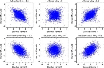
In addition, Figure 1 illustrates the difference between the two-dimensional t 3 copula (with v=3 degrees of freedom) and Gaussian copula, i.e., t v with v→ ∞, for normal marginals and varying strengths of dependence. (In this particular instance, the three-dimensional plots provide no new insights.) Notice how the tail dependence manifests itself for v=3 and disappears as v→ ∞, i.e., in the latter case there are essentially no points in the corners of each plot.
Two-dimensional copula realisations for negatively dependent, zero dependent, and moderately positively dependent normal marginals. Top row: t 3 copulas. Bottom row: Gaussian copulas.

3. Risk Measures
Risk measure is a useful tool for quantifying the riskiness of a portfolio, and we shall use a special type of coherent risk measures for this study. More specifically, in order to compare the riskiness of portfolios, spectral risk measures will be utilised. Such measures were first introduced in the finance literature with the intention that the user may wish to re-weight the initial distribution of the portfolio in order to reflect his/her risk aversion. In mathematical terms, a spectral risk measure R=R[F] of a random variable X, with a cdf F, is defined as
 $$R{\rm [}F{\rm ]\,{\equals}\,}{\int}_0^1 {F^{{{\minus}{\rm 1}}} {\rm (}u{\rm )}J{\rm (}u{\rm )}\:du} $$
where J is the weight function which controls the risk aversion, and F −1 the quantile function of X. Choosing the weight function J(u)=1 for 0≤u≤1, in equation (3.1), gives the expected value of X (denoted by mean[F]); J(u)=r(1−u) r−1 for 0≤u≤1 yields the proportional hazards transform of F (denoted by pht[F]), where r (0<r≤1) is a real-valued constant known as the distortion level; and conditional tail expectation of F (denoted by cte[F]) can be defined as spectral risk measure by setting J(u)=0 for 0≤u<t and J(u)=1/(1−t) for t≤u≤1, where t (0≤t<1) is a real-valued constant known as the threshold level.
In practice, the cdf F has to be estimated from the observed data. As discussed in section 1, one can do that parametrically, non-parametrically, or semi-parametrically and then insert the estimated F in equation (3.1), which would produce an estimator of R[F]. In this paper, we will focus on the empirical non-parametric estimation, i.e., in (3.1) we replace F by the empirical cdf
 $\widehat{F}_{n} $
. That leads to the following formula for the empirical estimator of a risk measure R[F]:
 $$R[\widehat{F}_{n} ]\,{\equals}\,\mathop{\sum}\limits_{j{\equals}1}^n {c_{{jn}} X_{{j\,\colon\,n}} } $$
where X
1:n
≤ ⋯ ≤X
n:n
denote the ordered values of data X
1, … , X
n
, and
 $c_{{jn}} {\rm \,{\equals}\,}{\int}_{(j{\minus}1)\,/\,n}^{j\,/\,n} {\,J{\rm (}u{\rm )}du} $
. Note that
 $R[\widehat{F}_{n} ]$
, as defined in (3.2), belongs to a general class of L-statistics, theoretical properties of which are well understood and have been thoroughly studied by Jones & Zitikis (Reference Jones, Puri and Zitikis2003, 2007), Necir & Meraghni (Reference Necir and Meraghni2009, Reference Necir and Meraghni2010), and other authors.
4. Hypothesis Test
4.1. Problem formulation
Let X(1), … , X(k) denote k (independent or dependent) portfolios of risks with cdfs F 1, … , F k , respectively. Suppose their riskiness is measured using the risk measures R 1=R[F 1], … , R k =R[F k ], as defined by (3.1). The hypothesis of interest is to check whether or not the k risk measures are all equal. That is, we formulate the problem as follows:
 $$H_{{\rm 0}} {\rm \,\colon\,}\,R_{1} {\rm {\equals}} \cdots \,{\rm {\equals}\,}R_{k} \quad {\rm versus}\:\quad H_{{\rm A}} {\rm \,\colon\,}\:{\rm at}\;{\rm least}\;{\rm one}\;{\rm pair}\,R_{i} \,\ne\,R_{j} $$
To test the above hypothesis, Brazauskas et al. (Reference Brazauskas, Jones, Puri and Zitikis2007) proposed a non-parametric test statistic that constructs the Gini index based on R 1, … , R k . Hence, all information about the differences of portfolio riskiness can be summarised by the inequality index
 $$\gamma \,{\rm {\equals}\,}{{\rm 1} \over {k^{2} }}\mathop{\sum}\limits_{1\leq i,\,j\leq k} \left| {R_{i} {\minus}R_{j} } \right|{\rm \,{\equals}\,}{{\rm 1} \over {k^{{\rm 2}} }}\mathop{\sum}\limits_{i{\rm \,{\equals}\,1}}^k {\rm (4}i\,{\minus}\,{\rm 2(}k{\rm {\plus}1))}R_{{i{\rm \,\colon\,}k}} $$
where the second equality follows from a well-known result for order statistics (see, e.g. David & Nagaraja, Reference David and Nagaraja2003, section 9.4), and R 1:k ≤ ⋯ ≤R k:k denote the ordered values of R 1, … , R k . This leads to a more compact formulation of the problem:
 $$H_{{\rm 0}} {\rm \,\colon\,}\,\gamma {\rm \,{\equals}\,0}\;{\rm versus}\;H_{{\rm A}} {\rm \,\colon\,}\,\gamma {\rm \,\gt\, 0}$$
4.2. Test statistic
A natural way to estimate γ is to replace R
i:k
with
 $\widehat{R}_{{i\,\colon\,k}} $
in (4.1), which yields
 $$\widehat{\gamma }\,{\equals}\,{1 \over {k^{{\rm 2}} }}\mathop{\sum}\limits_{i\,{\equals}\,{\rm 1}}^k (4i\,{\minus}\,2(k{\plus}1))\widehat{R}_{{i\,\colon\,k}} $$
That is,
 $\widehat{\gamma }$
is defined as an L-statistic based on ordered values of
 $\widehat{R}_{1} ,\,\ldots\,,\,\widehat{R}_{k} $
, each of which is an L-statistic itself (see equation (3.2)). Now we can see that
 $\widehat{\gamma }$
is an L-statistic of L-statistics, hence the name “nested L-statistic”.
To test the hypothesis stated in section 4.1, the following test statistic was proposed:
 $$T\,{\equals}\,{{\widehat{\gamma }} \over {\sqrt {\mathop{\sum}\limits_{i\,{\equals}\,1}^k {n_{i}^{{{\minus}1}} } } }}$$
where
 $\widehat{\gamma }$
is defined by (4.2) and n
i
the sample size generated by portfolio X(i) with cdf F
i
. Asymptotic properties of the test statistic T are established in section 2 of Brazauskas et al. (Reference Brazauskas, Jones, Puri and Zitikis2007). Those results, however, are too complicated for practical decision making, i.e., closed form expressions for critical values of the test are difficult to obtain. Therefore, it was suggested to use a bootstrap approximation instead.
4.3. Decision making
To accommodate portfolio dependence using copulas, we will assume that all sample sizes are equal, i.e., n 1=⋯=n k =n. Next, for 1≤j≤n, let (X j (1), … , X j (k)) denote the jth realisation of the dependent random vector (X(1), … , X(k)). Then, using sampling with replacement, we obtain the bootstrap samples (marked with a superscript “*”) such that
 $$(X_{1}^{{\asterisk}} (1),\,\ldots\,,X_{1}^{{\asterisk}} (k))\,{\equals}\,(X_{{j1}} (1),\,\ldots\,,X_{{j1}} (k)),\,\,\ldots\!\ldots\,,\,(X_{n}^{{\asterisk}} (1),\,\ldots\,,X_{n}^{{\asterisk}} (k))\,{\equals}\,(X_{{jn}} (1),\,\ldots\,,X_{{jn}} (k))$$
Further, using these resampled observations, we can compute the bootstrap estimate
 $\widehat{R}_{i}^{{\asterisk}} $
of
 $\widehat{R}_{i} $
, for every 1≤i≤k, by replacing X
j:n
with
 $X_{{j\,\colon\,n}}^{{\asterisk}} (i)$
in formula (3.2). After that, the bootstrap estimate of the Gini index γ is calculated using the following relationship:
 $$\widehat{\gamma }^{{\asterisk}} {\equals}\mathop{\sum}\limits_{i\,{\equals}\,1}^k \left( {4i\,{\minus}\,2(k{\rm {\plus}}1)} \right)D_{{i\,\colon\,k}}^{{\asterisk}} $$
where
 $D_{{1\,\colon\,k}}^{{\asterisk}} \leq \cdots \leq D_{{k\,\colon\,k}}^{{\asterisk}} $
are ordered values of
 $D_{i}^{{\asterisk}} {\rm \,{\equals}\,}\widehat{R}_{i}^{{\asterisk}} {\minus}\widehat{R}_{i} $
, for i=1, … , k. Combining these evaluations together, the bootstrap version of the test statistic T is given by
 $$T^{{\asterisk}} {\equals}\sqrt {{n \over k}} \,\widehat{\gamma }^{{\asterisk}} $$
Finally, we repeat the above resampling procedure B times and in this way obtain B replicates of T*, denoted as
 $T_{1}^{{\asterisk}} ,\,\ldots\,,T_{B}^{{\asterisk}} $
. The bootstrap estimate of the critical value of the test is the (1−α) level quantile of T*, denoted by x
α
[T*]. It can be estimated by
 $T_{{\left\lfloor {B(1{\minus}\alpha )} \right\rfloor \,\colon\,B}}^{{\asterisk}} $
, the
 $$\left\lfloor {B(1{\minus}\alpha )} \right\rfloor {\rm th}$$
order statistic of T*. The decision rule is as follows: we reject the null hypothesis H
0 in favour of the alternative hypothesis H
A if the actual value of the test statistic T (the value obtained from the original samples) exceeds the approximated critical value x
α
[T*]. Otherwise, we do not reject H
0.
5. Simulation Study
Since the sampling distribution of the test statistic does not have a manageable closed form expression, we use Monte Carlo simulations to investigate how the performance of the test changes when insurance portfolios are dependent. More specifically, we are interested in quantifying the relationship between the power of the test and the strength of portfolio dependence, for selected types of alternatives. Note that the strength of dependence is modelled using t ν copula.
5.1. Study design
We first generate three dependent portfolios of insurance losses such that they are either equally risky (H 0 setting) or unequally risky (H A setting), according to a fixed risk measure. For this study, we choose mean, pht, and cte as the risk measures (see section 3). We then perform the hypothesis test of section 4 using the generated portfolios and compute its proportion of rejections. (Such a proportion estimates the nominal level of significance under H 0 and the power of the test under H A.) By executing this process for the four types of dependence listed in section 2 (negative dependence, zero dependence, moderate positive dependence, and strong positive dependence), we obtain the proportion of rejections corresponding to each of the dependence structures. Specific parameters and other details of the study design are described in sections 5.1.1 and 5.1.2.
5.1.1. Riskiness of portfolios
For generation of insurance portfolios with specified riskiness, we follow the simulation studies of Brazauskas & Kaiser (Reference Brazauskas, Jones, Puri and Zitikis2004), Kaiser & Brazauskas (Reference Kaiser and Brazauskas2006), Brazauskas et al. (Reference Brazauskas, Jones, Puri and Zitikis2007) and choose the following three parametric families:
-
∙ Exponential with the cdf
(5.1)
$$F_{1} {\rm (}x{\rm )}\,{\equals}\,{\rm 1}{\minus}e^{{{\minus}(x{\minus}x_{0}{)\,/\,\theta } }} ,\;\;x\,\gt\,x_{{\rm 0}} ,\,\theta \,\gt\,0$$
-
∙ Pareto with the cdf
(5.2)
$$F_{2} {\rm (}x{\rm )\,{\equals}\,}1{\minus}(x_{0} \,/\,x{\rm )}^{\beta } ,\;\;x\,\gt\,x_{0} ,\,\beta \,\gt\,0$$
-
∙ Lognormal with the cdf
(5.3)where Φ(·) denotes the standard normal cdf.
$$F_{3} {\rm (}x{\rm )}\,{\equals}\,\Phi \,({\rm log}(x{\minus}x_{0} ){\minus}\mu ),\;\;x\,\gt\,x_{0} ,\,{\minus}\infty\,\lt\,\mu \,\lt\,\infty$$
The parameter x 0 in the above distributions can be interpreted as a deductible or a retention level of an insurance policy. (Note that due to x 0, the distributions F 1, F 2, and F 3 have the same support.) Although in general x 0 could be any positive real number, for this study we set x 0=1. The other parameters θ, β, and μ are selected in such a way that the cdfs F 1, F 2, and F 3 follow the hypothesised portfolio riskiness with respect to a fixed risk measure. In particular, if they are equally risky (under H 0), then they must satisfy the equation
(5.4)
$$R[F_{1} ]\,{\equals}\,R[F_{2} ]\,{\equals}\,R[F_{3} ]$$
where R[·] represents either mean, pht, or cte. (These are three conceptually different risk measures – mean is a measure of central tendency; pht and cte are tail measures but defined using different probabilistic principles – that allow us to judge sensitivity of the decisions to the choice of risk measure.) Evaluation of these measures for the distributions F 1, F 2, and F 3 yields the following expressions of (5.4).
-
∙ For the mean risk measure (when R[F i ]=mean[F i ]):
(5.5)
$$x_{0} {\plus}\theta \,{\equals}\,{{x_{0} \beta } \over {\beta {\minus}1}}\,{\equals}\,x_{0} {\plus}e^{{\mu {\plus}0.5}} $$
-
∙ For the pht risk measure (when R[F i ]=pht[F i ]):
(5.6)where for fixed r, the integral
$$x_{0} {\plus}{\theta \over r}\,{\equals}\,x_{0} {\plus}{{x_{0} } \over {r\beta {\minus}{\rm }1}}\,{\equals}\,x_{0} {\plus}C_{r} e^{\mu } $$
$C_{r} \,{\equals}\,{\int}_{{\minus}\infty}^\infty {\left( {1{\rm }{\minus}{\rm }\Phi (z)} \right)^{r} } e^{z} dz$
is found numerically. For example, as reported by Brazauskas & Kaiser (Reference Brazauskas, Jones, Puri and Zitikis2004), C
0.55=3.896, C
0.70=2.665, C
0.85=2.030, C
0.95=1.758. Note that when r=1, the pht measure becomes the mean.
-
∙ For the cte risk measure (when R[F i ]=cte[F i ]):
(5.7)
$$x_{0} {\minus}\theta ({\rm log(}1{\minus}t{\rm )}{\minus}1){\equals}{{x_{0} \beta } \over {\beta {\minus}1}}(1{\minus}t)^{{{\minus}1\,/\,\beta }} \,{\equals}\,x_{0} {\plus}{1 \over {1{\minus}t}}e^{{\mu {\plus}0.5}} \Phi (1{\minus}\Phi ^{{{\minus}1}} (t))$$
Note that when t=0, the cte measure becomes the mean.
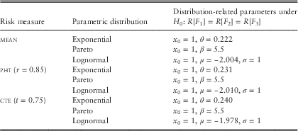
For the simulation study we fix x 0=1 and β=5.5, and then compute the corresponding values of θ and μ for each risk measure. Table 1 provides all distribution-related parameters under H 0, which are calculated using equations (5.5)–(5.7).
Under H A, the riskiness of portfolios can be unequal in numerous ways. In this study, we consider the following two types of alternatives:
-
∙ Two portfolios are equally risky but the third one differs; i.e.
(5.8)where
$$R[F_{1}^{{\asterisk}} ]\,{\equals}\,c_{{\asterisk}} R[F_{1} ],\,R[F_{2}^{{\asterisk}} ]\,{\equals}\,R[F_{2} ],\,R[F_{3}^{{\asterisk}} ]\,{\equals}\,R[F_{3} ]$$
$$F_{1}^{{\asterisk}} ,F_{2}^{{\asterisk}} ,\,{\rm and}\,F_{3}^{{\asterisk}} $$
are parametric distributions of portfolios under this alternative,
$ c_{\ast}$
≠1, and R[F
1]=R[F
2]=R[F
3].
-
∙ Relative riskiness of all three portfolios is equally spaced; i.e.


 $$R[F_{1}^{{{\asterisk}{\asterisk}}} ]\,{\equals}\,c_{{{\asterisk}{\asterisk}}} R[F_{1} ],\,R[F_{2}^{{{\asterisk}{\asterisk}}} ]\,{\equals}\,R[F_{2} ],\,R[F_{3}^{{{\asterisk}{\asterisk}}} ]\,{\equals}\,c_{{{\asterisk}{\asterisk}}}^{2} R[F_{3} ]$$
where
 $F_{1}^{{{\asterisk}{\asterisk}}} ,\,F_{2}^{{{\asterisk}{\asterisk}}} ,\,{\rm and}\,F_{3}^{{{\asterisk}{\asterisk}}} $
are parametric distributions of portfolios under this alternative,
 $ c_{\ast\ast}$
>1, and R[F
1]=R[F
2]=R[F
3].
The risk measure and distribution-related parameters under H 0.

pht, proportional hazards transform; cte, conditional tail expectation.
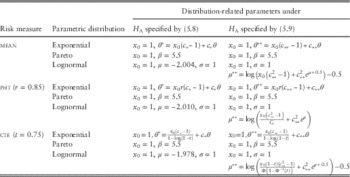
To simulate these scenarios, we choose parameters θ and μ to be identical to their values under H 0. Also, constants c * and c ** are such that c *=0.85, 0.90, 0.95, 1.05, 1.10, 1.15, 1.25 and c **=1.05, 1.10, 1.15, 1.20, 1.25. The remaining distribution-related parameters are derived from equations (5.8) and (5.9), and their values or formulas are presented in Table 2.
The risk measure and distribution-related parameters under H A.

pht, proportional hazards transform; cte, conditional tail expectation.
5.1.2. Dependence of portfolios
This section presents algorithms and major steps for generation of dependent portfolios with exponential, Pareto, and lognormal margins and the dependence structures specified by the correlation matrices of section 2. Briefly, a key idea is to use the meta-t ν distribution which is a multivariate distribution with arbitrary margins and the dependence structure governed by t ν copula. In our examples, the degrees of freedom parameter is either ν=3 or ν→∞ (the latter case corresponds to the meta-Gaussian distribution). Specifically, we implement the following three-step procedure:
Step 1. For a fixed risk measure and a fixed scenario of riskiness, we first generate a random realisation of the trivariate variable t ν , with the location vector 0 and the correlation matrix Σ (examples of which are specified in section 2). The sample size of each margin is n, and we denote this variable as Y=(Y 1, Y 2, Y 3).
Step 2. Next, we transform Y into U=(U 1, U 2, U 3)=(G ν (Y 1), G ν (Y 2), G ν (Y 3)), where G ν is the cdf of the standard t ν variable (i.e. with location 0 and scale 1). The distribution of U is the trivariate t ν copula with the correlation matrix Σ.
Step 3. Finally, as the well-known Sklar’s theorem ensures, the quantile transformation of the uniform margins returns the output with the desired probabilistic features. That is, the trivariate vector
 ${\bf X}{\rm \,{\equals}\,(}X_{{\rm 1}} {\rm ,}\,X_{{\rm 2}} {\rm ,}\,X_{{\rm 3}} {\rm )\,{\equals}\,(}F_{1}^{{{\minus}1}} {\rm (}U_{{\rm 1}} {\rm ),}\,F_{2}^{{{\minus}1}} {\rm (}U_{{\rm 2}} {\rm ),}\,F_{3}^{{{\minus}1}} {\rm (}U_{{\rm 3}} {\rm ))}$
, where
 $F_{1}^{{{\minus}1}} {\rm (}u{\rm )}\,{\equals}\,x_{0} \,{\minus}\,\theta \,{\rm log}(1{\minus}u),\,F_{2}^{{{\minus}1}} (u)\,{\equals}\,x_{0} (1{\minus}u)^{{{\minus}1\,/\,\beta }} ,\,F_{3}^{{{\minus}1}} (u)\,{\equals}\,x_{0} {\plus}{\rm exp}(\Phi ^{{{\minus}1}} (u){\plus}\mu )$
represents portfolios X
1, X
2, X
3 with marginal cdfs F
1, F
2, F
3, defined by (5.1)–(5.3), and their interdependence governed by t
ν
copula with the correlation matrix Σ.
Further, since t ν copula is fully characterised by its correlation matrix Σ, one can easily see that setting Σ equal to Σ1, Σ2, Σ3, or Σ4 (see section 2) in Step 1 produces portfolio realisations with negative dependence, zero dependence, moderate positive dependence, or strong positive dependence, respectively. Also, to generate equally and unequally risky portfolios, we change the parameters of the quantile functions according to the specifications of Tables 1 and 2, respectively.
Finally, while Steps 2 and 3 are straightforward transformations of random variables, Step 1 requires a more careful explanation. For Σs with non-diagonal elements strictly <1, we generate the trivariate variable t ν (with the location vector 0) by implementing Algorithm 5.2 of Embrechts et al. (Reference Embrechts, Lindskog and McNeil2003):
-
(a) Find the Cholesky decomposition M of Σ.
-
(b) Simulate three independent standard normal random variables Z 1, Z 2, Z 3.
-
(c) Simulate a random variable V from
$\chi _{v}^{2} $
that is independent of
Z
=(Z
1, Z
2, Z
3). -
(d) Then
${\bf Y}{\equals}\sqrt {\nu \,/\,V} \,M{\bf Z}$
is the trivariate t
ν
variable with location 0 and correlation Σ.


In the case when ν→∞, the (c) step can be skipped and the transformation of variables in (d) replaced with Y=M
Z. This results in the trivariate Gaussian variable with location 0 and correlation Σ. In addition, for commonotonic cases (e.g. Σ4 in section 2), the tail dependence differences between the t
ν
and Gaussian copulas vanish (see McNeil et al., Reference McNeil, Frey and Embrechts2005, section 5.3.1). Thus, the strong positively dependent portfolios can be generated by ignoring Steps 1 and 2 and modifying Step 3 as follows: simulate a standard uniform random variable U and then compute
 ${\bf X}\,{\equals}\,(F_{1}^{{{\minus}1}} (U),\,F_{2}^{{{\minus}1}} (U),\,F_{3}^{{{\minus}1}} (U))$
, where
 $F_{1}^{{{\minus}1}} ,\,F_{2}^{{{\minus}1}} ,\,F_{3}^{{{\minus}1}} $
are defined as in Step 3 above (see McNeil et al., Reference McNeil, Frey and Embrechts2005, proposition 5.16). For alternative specifications of the algorithms of this section, see Joe (Reference Joe2014, sections 6.9 and 2.5).
5.2. Numerical findings
Once a set of portfolios is generated then they are resampled according to the bootstrap procedure of section 4.3, an α-level test is performed, and its decision – reject H
0 or not – is recorded. This procedure is repeated 5,000 times, for each of the three risk measures, four dependence structures, and for each of the hypothesised scenarios. Using the recorded 5,000 decisions for the tests based on the mean, pht, and cte measures, respectively, we estimate the proportion
 $\widehat{p}$
of test’s rejections. Under H
0, if
 $\widehat{p}$
falls within the 99% confidence interval
 $\alpha \,\pm\,z_{{0.005}} \sqrt {\alpha (1{\minus}\alpha )\,/\,5,\!000} $
, where z
0.005 is a critical value of the standard normal variable, then the test performs as expected. If
 $\widehat{p}$
exceeds the upper bound of the interval, then the test is labelled as liberal. And if it is below the lower bound, then the test is called conservative. The study is performed for the following choices of simulation parameters:
-
∙ Level of significance: α=0.01, 0.05, 0.10.
-
∙ Sample size: n=50, 100, 200.
-
∙ Number of bootstrap samples: B=1,000.
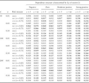
Our simulation results are summarised in Table 3, where probabilities of type I error are reported, as well as in Figures 2 and 3, where estimated power curves are plotted. Specifically, we notice from Table 3 that in the presence of strong positive dependence (comonotonicity), the probability of the type I error exceeds the nominal level several times, sometimes even more than ten times (see, e.g. the entries for α=0.01), for all the risk measures under consideration. This means that the test is very liberal under this scenario of dependence, which is most extreme. For the less extreme strengths of dependence, however, the results are mixed. That is, they depend on the chosen risk measure (mean is never liberal, pht almost always, and cte sometimes), sample size (liberal performances are most common for n=50, less for n=100, and least for n=200), and even on the test’s significance level (for α=0.10, the bold entries are most frequent, but their frequency declines as α decreases). Further, outside of the comonotonic case, there is no statistical evidence to suggest that the strength of dependence monotonically affects the test’s level. Finally, except for several borderline cases, the effect of tail dependence is also undetectable (compare the corresponding entries for ν=3 and ν→∞).
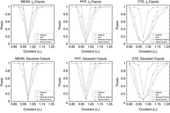
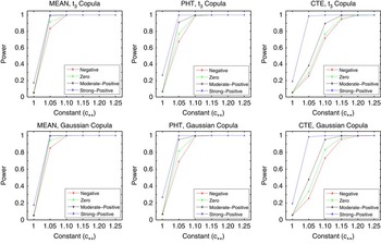
The first type of alternatives. Estimated power curves of the tests based on the mean, proportional hazards transform (pht), and conditional tail expectation (cte) measures, for various dependence structures, n=200, and α=0.05. Top row: t 3 copulas. Bottom row: Gaussian copulas.

The second type of alternatives. Estimated power curves of the tests based on the mean, proportional hazards transform (pht), and conditional tail expectation (cte) measures, for various dependence structures, n=200, and α=0.05. Top row: t 3 copulas. Bottom row: Gaussian copulas.

Estimated probabilities of the type I error of the tests based on the mean, proportional hazards transform (pht), conditional tail expectation (cte) measures, for selected n, α, ν, and various dependence structures.

Note: The 99% margins of error are ±0.004 (for α=0.01), ±0.008 (for α=0.05), ±0.011 (for α=0.10). The bold entries correspond to the cases when the test performance is liberal.
Figures 2 and 3 provide power estimates against the two types of alternatives described above, for n=200 and α=0.05. Similar to the type I error investigations, we notice that the power of the test is uniformly highest in the strong positive dependence case, for all risk measures and both types of copulas. Of course, this finding is not unexpected because the test exceeds the nominal level under H 0 and its power curve is simply shifted across all scenarios of riskiness. We also notice that the power of the test depends on the underlying risk measure. That is, all things being equal, the test is more powerful for the “light” measure (such as the mean) than for the “heavy” one (such as the pht or cte). There is no effect of tail dependence on the power curves, i.e., t 3 and Gaussian copulas produce similar power curves, but there is some effect of the strength of dependence. In particular, while negative dependence slightly decreases the power of the test when compared to the zero dependence case, the positive dependence improves the test’s performance. Other features of the estimated power curves are typical: the test becomes more powerful as c * (c **) moves further away from c *=1 (c **=1), i.e., when data go deeper into the alternative. Further, comparison of the two types of alternatives reveals that the test is more powerful against the second type of alternatives, which can be anticipated because under the second scenario the differences in portfolio riskiness are more pronounced. Finally, we conclude that the test – which was designed for independent portfolios – performs adequately when portfolios are dependent, and it will successfully detect, with the probability substantially above 0.50, the differences in portfolio riskiness of at least 15% (corresponding to c *≤0.85 or c *≥1.15, and c **≥1.15) for portfolios of n≥200 losses. Of course, a caveat to this conclusion is the comonotonic case which requires a separate analysis. (That is being carried out by the authors in a parallel paper.)
6. Practical Considerations
In this section, we illustrate how to apply the findings of section 5 in practice. Using the tornado damage data of Brooks & Doswell (Reference Brooks and Doswell2001), normalised values of which (i.e. data adjusted for wealth and inflation) are available in table A.3 of Brazauskas et al. (Reference Brazauskas, Jones, Puri and Zitikis2007), we reanalyse the real data example of the latter paper by investigating potential effects of portfolio dependence on the decision-making procedure.
The portfolios from given data are formed for two regions – Midwest and South – with the respective sample sizes n Midwest=47 and n South=86. (The data set also contains a third region, Northeast, but it has only four observations, which is way too small to assure valid statistical inference.) The hypothesis that the portfolios are equally risky was tested by applying the procedure of section 4. We used the same risk measures as in the simulation study: mean, pht (r=0.85), and cte (t=0.75). Also, B=1,000 bootstrap samples were generated to calculate the critical values at 1%, 5%, and 10% levels of significance. Table 4 provides summary estimates and decisions of the tornado damage data sorted by region.
Estimates and decisions for analysis of the tornado damage data sorted by region.

pht, proportional hazards transform; cte, conditional tail expectation.
Several conclusions emerge from the table. As the point estimates of all three risk measures suggest, the Midwest region is roughly twice as risky as the South. More formally, according to the mean measure, the difference is statistically significant at all typical levels of significance. And the pht (r=0.85) and cte (t=0.75) measures reject H 0 at α=0.05, 0.10 and α=0.10, respectively. Further, we need to check how sensitive these decisions are due to (potentially) misspecified portfolio dependence. Aside from the comonotonic case, the results of section 5.2 suggest that the decision to reject H 0 at the significance level α will remain at that level as long as portfolios are compared according to the mean measure. For the pht (r=0.85) and cte (t=0.75) measures, a premium of 20%–40% has to be added to α. That is, in many practical situations, the actual probability of type I error for pht (r=0.85) and cte (t=0.75) can reach 1.20α to 1.40α. Finally, the comonotonic case – no matter how rare it may be – represents a perfect-storm scenario that can break down the test and easily yield probabilities for the type I error as high as 0.30 or even higher. Thus the user of the test should keep such a possibility in mind.
7. Concluding Remarks
In this paper, we have considered a hypothesis testing problem about the equality of risk measures using a nested L-statistic. Asymptotic and small-sample properties of the test have been studied by Brazauskas et al. (Reference Brazauskas, Jones, Puri and Zitikis2007) under the assumption of independent insurance portfolios. Here, using Monte Carlo simulations, we have investigated the performance of the test when portfolios are dependent. We have concluded that the presence of strong positive dependence (comonotonicity) makes the test very liberal for the pht, cte, and mean risk measures, when marginal portfolios follow exponential, Pareto, and lognormal distributions and their interdependence is governed by the three-dimensional t and Gaussian copulas. For non-comonotonic scenarios of dependence, the test performs adequately, with its probabilities of type I error being on target for the mean measure and getting inflated by about 20%–40% for the pht and cte measures. In addition, for the alternative hypotheses considered in this paper, we have not observed any significant effects of tail dependence, but detected some effect of the strength of dependence. In particular, while negative dependence slightly decreases the power of the test when compared to the zero dependence case, the positive dependence improves the test’s performance. Finally, we have also demonstrated how to incorporate such findings into sensitivity analysis of the decisions by providing a real data example.
The results of this paper generate several ideas for further research. First, the comonotonic case has a devasting effect on the test and thus requires a separate analysis. Second, it is of interest to understand the mathematical phenomenon of how the power function of the test behaves due to changes in the correlation matrix that controls the interdependence of portfolios. This problem is related to various versions of stochastic ordering of random variables. Some preliminary results on this topic are reported by Samanthi et al. (Reference Samanthi, Wei and Brazauskas2016). Third, a natural extension of the test is to redesign it for discontinuous data that may include excessive number of zeros, but otherwise are continuous. (This is a common situation in personal lines insurance.) Going in this route, one would have to revisit the fundamental theorems on the asymptotic behaviour of L-statistics (see Chernoff et al., Reference Chernoff, Gastwirth and Jones1967). Fourth, one may abandon the idea of using the Gini index on risk measures and construct a completely different test. There may, of course, be many more generalisations and improvements of the approach presented in this paper.
Acknowledgements
The authors are very appreciative of useful comments and valuable insights provided by an anonymous referee that helped to improve the paper. Also, the second author gratefully acknowledges the support provided by a startup grant from the University of Wisconsin-Milwaukee.