Why are public finances important? Why study provincial own-source revenues?

The volume of a state's revenues and expenditures determines what it can do and how much of it. The singular innovation of governments in affluent societies after World War II was in the amount of revenues they extracted from their economies in peacetime and their decision to direct these new sums mostly to social measures. Government expenditures in the average OECD nation rose from 27.9 to 42.6 per cent of GDP between 1960 and 1980. The same years witnessed a shift in resources towards welfare states; social expenditures, excluding education, rose from an average of 36.1 per cent of public spending in 1960 to 52.4 per cent in 1998 (Castles, Reference Castles2004: 29, 33). If public education spending is included, welfare states accounted for about 66 per cent of public outlays in the latter year.Footnote ² Social spending defined in these broad terms also predominated in the Canadian provinces. In 2006–2007 it absorbed 66.3 per cent of expenditures in Quebec, and 68.1 per cent in Ontario.Footnote ³

The post-1980 years witnessed a levelling off of revenues in OECD nations. This was accompanied by an apparent incapacity of governments to restrain expenditures as much as taxes, resulting in sharply rising public debt in many of these nations, and calling into question the sustainability of welfare states (Pierson, Reference Pierson and Pierson2001; Streeck, Reference Streeck2014).

Are these patterns mirrored in the Canadian provinces? And why study the provinces if one is concerned about Canadian public finances? The second question is addressed first. Provinces now raise most revenues in Canada, and administer most of its social measures. In 1961, 51.5 per cent of all revenues were raised and spent by the federal government; an additional 10.5 per cent were raised by Ottawa but transferred to the provinces. Only 38.4 per cent consisted of provincial own-source revenues, monies raised and spent by the provinces or their municipalities. By 2008, the federally expended share had fallen to 32.4 per cent, transfers took up 11.5 per cent, and provincial own-source revenues were 56.1 per cent.Footnote ⁴ Most revenues are now raised by the provinces; around two-thirds are expended by them. Canada may now exceed all other federations in its degree of fiscal decentralization to the second tier of government (Haddow, Reference Haddow2015: 29–34). To discuss Canadian revenues is, predominantly, to discuss provincial revenues.

The rest of this section portrays provincial fiscal trends since the 1960s. Most of the data derive from Statistics Canada's Financial Management System (FMS), the best source for provincial finances. But the FMS was terminated in 2008. At the time of writing, it had not been replaced by an alternative that is fully comparable or that reports consolidated provincial data. The regression results reported later therefore cover the years 1981 to 2008. Statistics Canada is replacing the FMS with Canadian Government Finance Statistics (CGFS). In its preliminary form this has been used here to calculate reasonably comparable figures for debt and own-source revenues from 2008 to 2012. These are reported in this section's graphs to suggest how these aggregates evolved after 2008.

Figure 1 reports mean provincial total revenues and expenditures (graph i); and average debt (graph ii). For the provinces, like the OECD nations, a period of dramatic fiscal expansion after World War II ended by the mid-1990s. Average revenues rose from 19.3 per cent of GDP in 1965 to 32.6 per cent in 1994. They then declined to 27.9 per cent in 2003. Thereafter, they remained largely unchanged: 28.0 per cent in 2008 and about the same, according to CGFS data (not shown) in 2012.

Figure 1

Mean Provincial Revenues, Expenditures and Debt

Source: See appendix A

But the provinces differ fundamentally from the OECD regarding debt. Average spending often exceeded mean revenues before each peaked (graph i). Thereafter revenues generally matched expenditures. Consequently, a period of sharply rising debt until the 1990s was followed by one of steep decline, made possible by economic growth and balanced budgets (graph ii). After the financial crisis most provinces adopted stimulus strategies that saw their debts rise again. But three provinces had already returned to balanced budgets in 2014–2015; four more expected to join them by 2016–2017.Footnote ⁵ Thus, the post-crisis uptick in provincial debt is likely to end long before it returns to mid-1990s levels. In contrast with the OECD, then, stagnant, sometimes declining, revenues were not accompanied by ever-rising debt because expenditures broadly fell as fast as revenues. Provincial revenues shrank in the new era, but provincial finances are not unsustainable.

Revenues, not the prospect of fiscal crisis, therefore, are the focus of this study. Why choose own-source over total revenues or expenditures? Total revenues include federal transfer payments, which are also an important determinant of spending. These transfers form a very uneven proportion of revenues for different provinces. Regression analyses can control for their influence by including an IV for transfers. But much evidence discussed here relies on descriptive data, where direct observation is made of levels for relevant indicators. In addition, the regression procedure discussed below requires rotating groups of IVs through different models, with none present in all of them. Finally, own-source revenues offer the most direct evidence of variations among jurisdictions and over time in their efforts to raise the funds needed to pursue public purposes.

Average provincial own-source revenues since 1965 are depicted in Figure 2, graph (i). This mean rose from 13.8 to 20.6 per cent of GDP between 1965 and 1980, and to 24.5 per cent in 1994. It then fell to 21.6 per cent in 2004 and 20.9 per cent in 2008 but rebounded after the financial crisis to 21.6 per cent in 2012. As with total revenues, growth until the 1990s was followed by a decade of decline and by little change recently. Average own-source revenue levels in 2012 were around their 1980 level. An era of rapid expansion again juxtaposes with later periods of decline and stasis.

Figure 2

Mean Provincial Own-Source Revenues

Source: See appendix A

Yet this average pattern conceals major variations. Figure 3 traces the evolution of own-source revenues for each province. Graph (ii) in figure 2 reports their standard deviation. Interprovincial variations have fluctuated, but the broad trend is upwards since the early 1990s. The standard deviation rose from 1.4 in 1991 to 2.9 in 2012. If we set aside 2006 to 2008, when the deviation briefly exceeded 3, the post-1991 years appear as an era of gradually increasing variation in provincial revenue levels.

Figure 3

Own-Source Revenues, 10 Provinces, 1965–2012

Source: See appendix A

Provincial levels also followed very different trajectories. Alberta's revenue ratio was the highest in 1965; but the size of its tax state peaked before 1980, then commenced a protracted decline. In 2008, Alberta had the second-lowest level. Revenue shares continued to rise in Saskatchewan and Newfoundland until 1989 and 1996, respectively, before also declining sharply; they rebounded in the latter province after 2008. After 2000, these three provinces were Canada's leading energy producers and benefited from buoyant commodity markets.Footnote ⁶ In the face of this windfall, they did not increase spending, and the revenues needed to finance it, perhaps afraid of not being able to continue doing so if energy prices fell. But provinces that do not rely heavily on natural resource royalties did not experience declines of the same magnitude. New Brunswick, Manitoba and British Columbia also saw a retreat in revenue levels after the 1990s, but a smaller one. In contrast, own-source revenues have not receded notably in Ontario and Quebec, Canada's most populous provinces, and have also experienced no significant drop in Nova Scotia or PEI.

This heterogeneity suggests that the influences shaping revenues after 1980 affected provinces very differently. What are these influences? The next section addresses the main explanations offered by CPE scholars for variations in states’ fiscal aggregates, and in the welfare states they pay for. This review is the basis for the hypotheses tested later.

Literature review: Taxes, expenditures and welfare states

During the 1950s and 1960s the most influential explanation of post-war state expansion was that it responded to changing societal needs in the wake of industrialization and rising affluence (Wilensky and Lebeaux, Reference Wilensky and Lebeaux1958). Three decades later, this “modernization” theory no longer predominated. Scholars now concentrated on explaining the sizable differences among welfare states and, later, on whether they would persist. That well-financed welfare states must also be rich nevertheless is now more presupposed than rejected.

The “power resources” perspective (PR) emerged as a leading account of variation.Footnote ⁷ It contends that the size and redistributive impact of welfare states is conditioned by the power balance between labour and its centre-left partisan allies, on the one hand, and rival, perhaps business-aligned, parties, on the other. Where the left grows stronger, it obtains more ample redistributive measures for its less-advantaged constituency. The left's influence is exercised in the long term. For Korpi, it required “long-term changes” in the balance of power, and “strong and stable control over government” (Reference Korpi1980: 309). Esping-Andersen added that social programmes, once implemented, enhance the power of the interests that legislated them by attracting the loyalty of beneficiaries to their distributive preferences. Thus, liberal and conservative welfare state regimes, each incongruent with the left's egalitarianism, became “major historical impediments to social democratic reformism” (Reference Esping-Andesen1985: 231). Conversely, where social democrats governed frequently and implemented egalitarian programmes, they benefited later from the “solidarity” that these measures embodied (Reference Esping-Andesen1985: 238). These processes are well described by Pierson's subsequently elaborated concept of “path dependence”: long-term and “self-reinforcing or positive feedback processes,” which, once underway, “make reversals very difficult” (Reference Pierson2004: 10, 95).

Quantitative PR researchers usually employ estimation strategies designed to measure this long-term impact, though there is considerable heterogeneity in the specific methods used. Huber and Stephens measured variables in levels, not first differences; and pooled data from different national cross-sections, rather than estimating with fixed effects (FEs) (Reference Huber and Stephens2001: 35–36, 57–62). Variables in levels enter models in their natural units. Most of those used in macro-level CPE scholarship change only slowly; they are path-dependent. In contrast to levels estimation, first differencing (FD) measures changes in variables’ values between time periods. Regressions then measure how much change in the DV is associated with this short-term change in the IVs.

In mature political economies, well-established paths entail that levels for many variables may differ considerably between countries. When TSCS data are pooled in levels regressions, long-term, cross-national differences are estimated based on these differences, as are over-time variations within countries. FE estimation, in contrast, measures the latter, but not the former. Moreover, these temporal effects are short-term, though estimated differently than in FD models.Footnote ⁸ Kennedy refers to the resulting paradox for TSCS data that “contrary to many people's intuition, cross-sectional data are said to estimate long-term relationships whereas time series data estimate short-term relationships” (Reference Kennedy2003: 308). Some PR scholars nevertheless estimate with FEs, but use interaction IVs or counterfactual analyses to measure cross-sectional differences.

There has been much debate about how to measure welfare state generosity. Use of the OECD's social security expenditures (SSEs) has long been contested. But alternatives have been slow to gain acceptance. The OECD data are still used widely (Scruggs, Reference Scruggs, Clasen and Siegel2007). As Kenworthy has shown, moreover, total public revenues and expenditures correlate highly with social spending measures (Reference Kenworthy2008: 176–77). Welfare state scholars therefore examine total revenues and expenditures, as well as SSEs. Using their recommended pooled regression in levels, Huber and Stephens found a significant impact for left incumbency on total revenues and expenditures during the post-war years, though not later (Reference Huber and Stephens2001: 68–69, 72–73). Also regressing in pooled levels, Hicks identified a strong influence for left cabinet control on SSEs (Reference Hicks1999: 172–73). These results were consistent with Esping-Andersen's, which focused entirely on the cross-sectional dimension, that partisanship shaped welfare state regimes (Reference Esping-Andersen1990: ch. 5). Cusack and colleagues’ levels analysis found that left governments responded to economic shocks by increasing SSEs more than right ones; they employed FEs, but measured cross-sectional variations with interactions (Reference Cusack, Iversen and Rehm2006: 382).

Scholars whose main interests lay outside of the welfare state also contributed to research on fiscal aggregates, again stressing the long term. Combining pooled data with a measure of revenue change over 15 years to capture a long-term pattern, Cameron argued that left incumbency contributed importantly to this change (Reference Cameron1978: 1254–58). Two decades later, Garrett found that “left labour power” was highly correlated with total government revenues; in interaction with capital mobility it also was significantly associated with total expenditures. His levels estimations included FEs, but used counterfactuals to identify cross-sectional variations. (Reference Garrett1998: 9, 80–84, 90–92). Boix detected distinctive conservative and social democratic economic strategies that, among other things, led left parties to choose higher levels of taxing and spending than right ones (Reference Garrett1998: esp, 53, 112–15, 165–67).

During the 1990s, economic globalization began to attract considerable attention; the term refers to several trends: rising levels of trade, capital flow and foreign domestic investment, and the widespread abandonment of capital controls (Simmons, Reference Simmons, Kitschelt, Lange, Marks and Stephens1999). Some early writing portrayed the state as largely helpless to prevent major reductions in its reach in globalization's wake. More nuanced later research supported claims about the importance of globalization with more careful specifications of how to measure it. For Busemeyer, “the process of economic internationalization proceeded and intensified during the 1980s and 1990s.” It should therefore be measured “in the over-time dimension” of TSCS data, not the “cross-sectional” one. Moreover, it was important to consider “changes in openness,” not their levels, because “we are looking at the effects of an ongoing, intensifying process of economic internationalization that differs substantially in character from the previous era” (Reference Busemeyer2009: 261; emphasis in original). In sharp contrast with PR dynamics, then, globalization is best measured temporally, not cross-sectionally; and in differences, not levels. It has a short-term influence, although its full impact requires an accumulation of short-term effects.

Accordingly, globalization scholars typically first difference all DVs and IVs, or estimate error correction models (ECMs), which regress a differenced DV on IVs in both levels and differences. Using both approaches, Busemeyer found a negative association between trade openness and total spending change between 1980 and 2004. He surmised that globalization only had this negative effect after 1980. He found no impact for left partisanship (Reference Busemeyer2009: 467–68, 472–73). Kwon and Pontusson also argued that the causal nexus had altered. Left partisanship was positively associated with annual differences in SSE during the 1980s, but not in the 1990s (Reference Kwon and Pontusson2010: 268, 272). Jensen found that globalization had a negative impact on changes in social transfers in liberal political economies, but not in co-ordinated ones; left partisanship had no influence (Reference Jensen2011: 178). Brady and Lee contended that until the 1980s union density strongly influenced annual differences in total expenditure. Thereafter, it did not; trade openness, adoption of the euro, unemployment and youth dependency all now suppressed spending (Reference Brady and Lee2014: 68–70).

An alternative account of threats to state fiscal capacity centres on postindustrialism. Disputing the importance of globalization, Pierson pointed instead to changes associated with the transition to a service economy. These include (i) a decline in productivity growth as tertiary-sector jobs displace industrial ones; (ii) higher unemployment if governments do not expand public sector employment; (iii) population aging; and (iv), evolving household structures, including rising female employment (Reference Pierson and Pierson2001: 83–86, 93–95). Each of these puts upward pressure on spending; some, especially the last, might also boost revenues. But the overall effect is likely to aggravate government debt, suggesting that revenues will not rise as fast as expenditures (90–92). Moreover, the beneficiaries of the welfare state now are its main support base; partisanship therefore is now much less important (Reference Pierson1996: 146–47). Postindustrialism is a process that unfolds in time and cumulatively, an “inexorable social process with major ramifications. Less dramatic and exotic than globalization, the shift to services nevertheless represents a profound social transformation” (Reference Pierson and Pierson2001: 87). In regressions, it is therefore likely to be measured with the same temporal strategy as is recommended for globalization. Thus, Iversen and Cusack used ECM estimation to detect a positive relationship between deindustrialization and public spending; left incumbency was much less important (Reference Iversen and Cusack2000: 333). Busemeyer (Reference Busemeyer2009: 469) found that postindustrial pressures promoted higher spending, whereas Brady and Lee came to the opposite conclusion (Reference Brady and Lee2014: 68–69). Postindustrialism's implications for revenues are uncertain. But if it suppresses the influence of partisanship, and either enhances or dampens spending, it may affect revenues. IVs that measure it therefore belong in the estimations presented below.

There is a scholarly literature on fiscal outcomes in the Canadian provinces. Pétry and colleagues found that public spending is lower when right parties govern in five provinces; this contradicted earlier findings of no partisan influence (Reference Pétry, Imbeau, Crête and Clavet1999: 284–86). Kneebone and McKenzie also reported that partisanship influenced provincial spending but determined that it did not affect revenues (Reference Kneebone and McKenzie2001: 761–62). Tellier concluded that left provincial governments spend more than others, but only when they are popular and not under severe budgetary constraints (Reference Tellier2006: 376). Tellier subsequently reported, like Kneebone and McKenzie, that total revenues were unaffected by partisan incumbency (Reference Tellier2009: 603). Pickup found that parties’ expenditure response to globalization differed depending on whether unionization was high or low (Reference Pickup2006: 900–02).

These Canadian studies arrived at different conclusions, although those that address revenues deny that partisanship affects them. Most were written a decade or more ago. With the exception of Pickup, their authors were mainly concerned with theories of political business cycles, not a focus here; they did not engage systematically with the CPE theories and methods discussed above. I am not aware of a study of provincial revenues or expenditures that examines the effects of partisanship, globalization and postindustrialism together. None of the scholars discussed in this section, comparative or Canadian, adopted the modelling strategy proposed below. The present contribution addresses these gaps.

Variable selection and methods

The CPE scholarship discussed above generated competing theories to explain state size. PR contends that revenues and expenditures reflect political conflict. Alternatives suggest that they are now conditioned by globalization or postindustrialism. Most globalization researchers, but not all, claim that it curtails state finances; postindustrial scholarship is more mixed. This article therefore tests for both upward and downward pressure from each, as well as for the ongoing relevance of politics. CPE scholars still examine the impact of economic and fiscal variables on state finances. But this study, like most contemporary ones, treats this fourth group of variables as controls. Three hypotheses are tested here, consistent with much recent scholarship: (i) partisanship does not shape provincial revenues after 1980; but (ii) globalization and (iii) postindustrialism do.

The above review also showed that TSCS methods appropriate for testing the first hypothesis may not be suitable for the second and third. PR claims that left influences are long term and path dependent. Most PR researchers adopt methods that highlight the cross-sectional dimension of TSCS data, and measure key variables in levels to capture this long-term dynamic. Globalization and postindustrialism, in contrast, unfold over time, with a rapid and cumulative impact. A focus on the temporal dimension, and estimation in the short term, using FEs, differencing or ECMs, is preferred. Cross-sectional analyses ignore time-dependent effects; temporal ones miss long-term influences.

It is in this context that multilevel estimation holds much promise; it bridges this gap. It is used in many fields to estimate the effect of IVs at two or more levels. In education research, for instance, models might include fixed (“within”) IVs that track individual student progress, and cross-sectional (“between”) ones that measure variations in progress at different schools. If cross-sections differ considerably, estimations are not biased because FEs are present in models. The estimation also avoids “confounding,” a danger in pooled regressions; a particular influence may affect students differently between and within schools (Begg and Parides, Reference Begg, Parides, Skrondal and Rabe-Hesketh2010). Only recently has multilevel estimation for macro-level TSCS data attracted advocates in political science (Bartels, Reference Bartels and Franzese2015; Bell and Jones, Reference Bell and Jones2015). Bell and Jones point out that employing FE estimation with TSCS data usually “means considering differences over time, controlling out higher-level [cross-sectional] differences and processes absolutely” (Reference Bell and Jones2015: 139). In contrast, multilevel estimation “separates … the within and between components of effects explicitly, and assesses how those effects vary over time and space rather than assuming heterogeneity away” (149). It therefore meets the present need to test theories of variation over time (globalization and postindustrialism) as well as space (power resources).

The dataset used here comprises 28 years of observations (1981 to 2008) for the ten provinces. Economic IVs include GDP per capita (gdp_pc) and interest payments on the public debt (debtpay).Footnote ⁹Fedtrans tracks federal transfer payments to the provinces. Trends in own-source revenues are affected by provincial energy rents (Figure 3); accordingly, minEnerg reports the share of provincial GDP generated by the mining and energy sector. This variable allows the regressions to control for the impact of resource income on provincial revenues, an influence whose importance was discussed above. Political variables include indicators for years of incumbency by three party groups: left, for the New Democratic Party and the Parti Québécois; centre for the Liberal party; and right for Progressive Conservatives, Social Credit and the Saskatchewan party. This is consistent with a CPE practice of clustering parties into ideological groups; the specific groups reflect a common Canadian practice (Pétry et al., Reference Pétry, Imbeau, Crête and Clavet1999: 283; Tellier, Reference Tellier2009: 601). To avoid collinearity only two indicators can be included in estimations; right is omitted as the reference category. Union density is measured by density.Footnote ¹⁰ Of globalization IVs used in CPE research, provincial data are available only for trade; fortunately, this is often the most statistically significant globalization IV (Busemeyer, Reference Busemeyer2009: 462–64). IVs are used for international (inttrade) and interprovincial (domtrade) trade. Variables are used for all four postindustrialism influences highlighted by Pierson (Reference Pierson and Pierson2001). Specifically, postindemp measures tertiary sector employment; femaleshare tracks women's’ employment; unemployment is the provincial unemployment rate; age is the share of the population older than 64.Footnote ¹¹ Consistent with common practice, all IVs are lagged one time period (Brady and Lee, Reference Brady and Lee2014: 63). Histograms were used to select the functional form of each continuous variable. They favoured the linear form for the DV, and for density, debtpay, postindemp, femaleshare and age; but a natural log form for inttrade, domtrade, unemployment, gdp_pc, fedtrans and minEnerg.

As is common with TSCS data, a modified Wald test rejected the null of homoscedasticity for all six models reported in Table 3; Pesaran's test identified panel-wise dependence in all continuous IVs, and in the DV. Estimation with panel corrected standard errors (PCSEs) accommodates both problems; it was employed for our main estimations. The Lagrange multiplier test additionally detected serial correlation in all models. A common response, use of a lagged dependent variable (LDV) was not adopted. LDVs bias TSCS estimations that include FEs, as ours do (Kennedy, Reference Kennedy2003: 313). This problem is instead addressed by means of first-order autocorrelation (AR1). To provide a robustness check on these estimations, the last four columns of Table 4 report joint significance test results for alternative estimations that employ GLS with Arellano cluster-robust standard errors (SEs) and OLS with Newey-West SEs.Footnote ¹²

The multilevel models include two versions of each IV: a time-invariant between one that comprises the mean level for each cross-section over 28 years; and a time-varying within (FE) one for annual variations in each cross-section around the mean.Footnote ¹³ Because they are time-invariant, only N-1, or nine, between IVs can be included in a regression. Moreover, exploratory estimations detected overfitting with eight or nine IV pairs. Variances and coefficients often were very large. To alleviate this, no more than seven pairs are included in any model, usually the maximum number in each combination of two IV groups.Footnote ¹⁴

The next section first reports bivariate correlations for each between and within IV and the DV, in Table 1. Results for separate regressions for the theoretically important IV groups are reported in Table 2, followed by results for each combination of two groups in Table 3. If there is evidence (i) that political IVs affect own-source revenue, we should expect to find this for the between versions of these IVs. Conversely, (ii) globalization or (iii) postindustrial impacts should be evident on the within dimension. Political variables might also have a short-term effect, reflected in within coefficients, but this is not our main expectation. Coefficients for time-invariant globalization and postindustrialism IVs may sometimes be statistically significant; but this cannot be understood as evidence of the processes examined here, which unfold in time. Between variants of these IVs nevertheless are included in regressions to avoid biasing their results. The overall influence of partisanship (left and centre parties), globalization and postindustrialism are of interest, as is the impact of specific aspects reflected in individual IVs. The first two data columns of Table 4, therefore, report joint significance scores for each group from the previous two tables.

These estimations are in levels; most globalization and postindustrialism scholarship (see above) is in first differences (FDs). In the econometric literature, FEs, the within part of our levels estimations, and FDs are treated as alternatives. Wooldridge recommends estimating both in many cases (Reference Wooldridge2006: 492). Both FD and ECM models therefore were estimated, those recommended by Busemeyer; these estimations included all IVs. These models are discussed below, but not presented here to conserve space. These check the robustness of the FE results for globalization and postindustrialism. But the preceding discussions suggest that they are not suitable for evaluating partisanship's long-term influence.

Findings

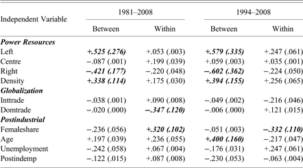
The R-squared is reported underneath each correlation coefficient in Table 1; it shows how much variation in the DV is explained by each IV. The first two data columns report results for 1981–2008, the last two for 1994–2008 when revenues declined. Regression models are not presented for the latter period alone; it is at the lower boundary of the more than 15 years that Beck recommends for accurate PCSE estimation (Reference Beck2001: 278). But the second set of correlations indicates whether the relationships examined here changed during these years of decline and stasis. Correlations are highlighted if their R-squared exceeds 10 per cent. To save space, between IVs are referred to here and in the tables with the suffix _bw, within ones with _wi.

Table 1

Bivariate Correlations of IVs with Own-Source Revenues / GDP (R-Squared in brackets)

These bivariate data indicate emphatically that power resources conditioned own-source provincial revenues very strongly after the Golden Age. The coefficients for left_bw and density_bw reveal a very positive relationship with revenues for our entire period; there is a strongly negative one for right_bw. For 1981–2008, left incumbency explains over a quarter of variation in revenues; right incumbency accounts for 18 per cent, density for 11 per cent. There is no strong impact for centre_bw. This is consistent with a PR perspective; there is no reason to expect parties in the ideological middle to shift state size in one direction or another. The last two columns suggest forcefully that these influences did not abate during the post-1994 era of fiscal retrenchment. Indeed, each correlation that is strong for the whole period strengthens during its second half; left_bw and right_bw now each account for a third or more of variation in revenues. Again consistent with PR expectations, finally, all of these strong correlations are on the path-dependent between dimension, not the short-term within one. Only for centre, where no R-squared exceeds 5 per cent, does the latter correlation once exceed the former.

The evidence is far more mixed for the globalization and postindustrial IVs. In four of six cases for the entire period the within correlation is stronger than the between one, as we expect. But only two of these explain over 10 per cent of variation for the whole period, only one for the post-1994 years. In the latter case (femealeshare_wi), moreover, the correlation reverses signs, suggesting very different relationships between IV and DV for the two halves of our study period. This evidence casts significant doubt on whether these IVs measure influences with a strong, cumulative over-time impact, as the theories reviewed earlier anticipate.

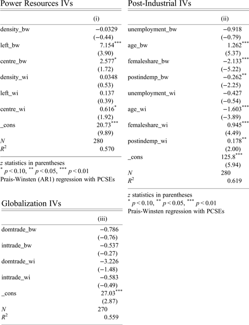
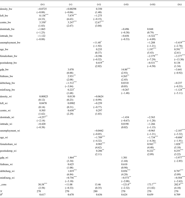
The discussion now turns to regression results. The estimation that includes only PR variables (model i of Table 2) and models (iv) and (v) in Table 3, which combine these with trade and economic IVs, strongly corroborate the bivariate evidence for left_bw. In all three cases, it is significant well above the 1 per cent level. Its coefficients in these models suggest that a province's own-source revenues would be about 7 per cent higher in a province where left parties governed throughout the 28 year period, compared to one where they never ruled. This is a very large effect; the standard deviation for the DV is 2.7, and its values range between 14 and 27 per cent of GDP. But left_bw's impact entirely disappears in model (vi), which combines political and postindustrial IVs; this result is discussed further below. The centre_bw variable is never as significant as left_bw in these cases, but it is associated with the DV in all four models. If one ignores the outlier coefficient in model (vi), moving from no centre government to centre's always being in power raises revenues in the long-term by about three percent of GDP. The density_bw variable is never significant. The between party IVs are jointly significant in the first three models (Table 4, first data column), always well above 1 per cent, but this result also disappears in model (vi). PR's impact is largely on the between dimension; the within-party IVs are never jointly significant, though centre_wi is in two of four models. With one exception, this overall pattern is very consistent with PR theory: left_bw has a much stronger impact, statistically and substantively, than centre_bw, but the latter is also significant in comparison with the right_bw reference IV. PR's effect is much greater in the long-term.

Table 2

Regressions of Own-Source Revenues / GDP on Individual IV Groups

z statistics in parentheses

^*p < 0.10, ^**p < 0.05, ^***p < 0.01

Prais-Winsten regression with PCSEs

Table 3

Regressions of Own-Source Revenues / GDP on Pairs of IV Groups

z statistics in parentheses

^*p < 0.10, ^**p < 0.05, ^***p < 0.01; Prais-Winsten Regression with PCSEs

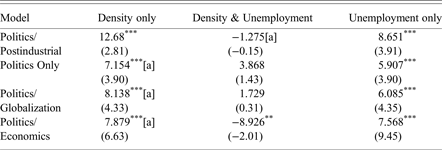
What, then, accounts for the non-significant result for left_bw in model (vi)? The left_bw variable is again significant if either unemployment_bw or density_bw is dropped from this model; its coefficients and significance levels in these cases are reported in the first row of Table 5. density_bw is very positively correlated with left_bw (+.543), and also with the DV (Table 1). unemployment_bw is very negatively correlated with left_bw (−.592), as it is with the DV. The density_bw variable is never significantly associated with the DV in a regression model when left_bw is present, despite its strong bivariate association with the DV. In density_bw's absence's unemployment_bw is negatively associated with the DV in model (vi), but only at 10 per cent (not shown). This pattern suggests that left_bw's impact, very pronounced in bivariate correlations and the first three models, nevertheless mediates the combined influence of long-term interprovincial differences in unionization and unemployment. Stronger unions foster higher own-source revenues, but this influence passes through long-term left incumbency. Conversely, where unemployment is higher in the long run, revenues are lower. This influence is also largely mediated by left incumbency; where unemployment is higher, left governments are less frequent. To test the robustness of this interpretation the first three political models (i and iv-v) each were rerun twice. The unemployment_bw variable was added in the first rerun; density_bw was dropped in the second. In all cases, as with model (vi), left_bw was not positively associated with the DV in the joint presence of the other two IVs, but was always significant above the 1 per cent level in the absence of one. These result are reported in the last three rows of Table 5. Their implications are discussed in the conclusion.

Table 4

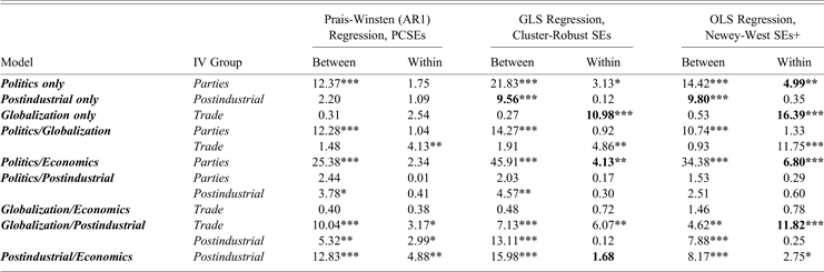
Tests of Joint Significance for IV Groups, Three Estimators

F-test or Chi-square coefficients

^*p < 0.10, ^**p < 0.05, ^***p < 0.01

+ Newey-West estimations included four lags

Table 5

Left_bw Coefficients for Alternative Configurations of Density & Unemployment IVs

t statistics in parentheses

^*p < 0.10, ^**p < 0.05, ^***p < 0.01

Coefficients marked [a] are from original models in tables 2 and 3

Results for the globalization and postindustrial IVs, in contrast, do not indicate that either group, as a whole, is strongly associated with own-source revenues. Model (iii) in Table 2, and models (iv), (vii) and (viii) in Table 3, include the trade IVs; models (ii), (vi), (viii) and (ix) contain postindustrial ones. Seven of eight coefficients for within trade IVs are negatively signed, as expected. But only domtade_wi in model (v) is significant. The trade variables are jointly significant on two of four occasions, but only at 10 per cent in one case. The ECM and differenced estimations do not modify this picture much. The inttrade variable's levels estimation is significant at 10 per cent in the former case; no other trade coefficient is significant in either model. Based on these results, we cannot be confident that greater trade, internationally or domestically, undermined provincial own sources revenues after 1980. If it did, they suggest that the impact was modest.

Within postindustrial IVs are much more likely to be significant. But the pattern is very heterogeneous, with different IVs having very distinct effects. The femaleshare_wi variable is positively associated with own-source revenues above the 1 per cent level in all four models, the most emphatic result for any IV. Increasing women's labour market participation raises revenues. Rising tertiary sector employment also contributes to higher revenues; postindemp_wi is always significantly and positively associated with the DV, at 5 per cent or higher. Yet age_wi has an equally powerful negative impact, significant in all four models, three times above 1 per cent; a rising share of elderly people suppresses revenues. In model (ix), unemployment_wi is also negatively associated with the DV. This highly mixed pattern entails that in two of these four models, (ii) and (viii), the within postindustrial IVs are not jointly significant (Table 4), suggesting that the individual IVs cancel each other out. When they are significant, it is at a much lower level than is often true for individual IVs: at 10 per cent in model (vii) and 5 per cent in model (ix). Their net impact is positive in these cases. The ECM and differenced model results corroborate that femaleshare and postindemp increase own-source revenues over time. They again indicate that unemployment lowers them. But the pattern observed for age in the multilevel estimations disappears here. Evidence about postindustrialism's impact overall is mixed, and probably contrary to trade's. If these two groups affected own-source revenues since 1980, according to these estimations, they may have offset each other. Finally, “confounding” is very evident for postindustrial IVs in models (vii), (viii) and (ix). In the first two of these, the sign for age, femaleshare and postindemp changes from the within to the between IV, and is now significant in the opposite direction. The same happens for age and femaleshare in model (ix).

In six of 24 cases joint tests from the alternative estimators disagree with PCSEs by two or more significance levels. (This would be the case, for instance, if an alternative found an IV group significant at 5 per cent when PCSEs identified no impact). These discrepancies are highlighted in the last four columns of Table 4. Four cases are especially pertinent here. The alternatives twice found the within party group significant when PCSEs did not (politics only and politics/economics models); and it was centre_wi’s coefficient, not left_wi's, that accounts for this. Yet both estimators gave much larger coefficients to the _bw joint test than the _wi one, and left_bw was much stronger in the between dimension. There is no contradiction here, then, to PR's expectation that partisanship's positive impact mostly is long term and from the left.

The alternative estimations for the trade variables raise a more substantial challenge. For the trade only and trade/postindustrial models, they both find the within trade variables much more significant. The domtrade_wi variable was (negatively) significant at 1 per cent in three of these four estimations, inttrade_wi twice (not shown). The within trade IVs were jointly associated with the DV for three of four models, at 1 or 5 per cent. These results suggest a stronger negative impact on own-source revenues than was reported above. This is consistent with globalization theory. Yet this evidence remains mixed. The correlation disappears in the trade/economics model; in the other two-variable-group estimations, z-values for the trade variables are always matched by several others.

Trade is a component of the broader phenomenon of economic globalization, the only one for which we have province-level data. The widely used KOF index measures globalization more comprehensively, but is available only for countries.Footnote ¹⁵ To see if it nevertheless helps explain provincial own-source revenues, especially during the post-1994 decline era, I compared correlations between Canadian levels for this index and the DV before and after 1994 with the same correlations for average trade levels. Mean domestic trade was already negatively correlated with own-source revenues before 1994. After 1994, the KOF correlation (−.140) is smaller than those for mean international (−.197) and interprovincial (−.375) trade. A more comprehensive globalization indicator therefore may do no better than trade data in explaining own-source revenues in this later period.