1 Introduction
The turbulent boundary layer is ubiquitous, occurring commonly in both nature and engineering applications. It is important in geophysical flows where better weather prediction models require more accurate representations of surface layer physics and in transportation where drag reduction could lower fuel costs and greenhouse gas emissions. The most important physical quantity characterizing wall-bounded turbulent boundary layers is the skin friction drag. The topic of experimental determination of skin friction drag is closely linked to a fundamental understanding of the total momentum balance in turbulent boundary layers. Much has been learned over a long history of research on these related topics and reviews of various skin friction determination techniques can be found in Winter (Reference Winter1979), Haritonidis (Reference Haritonidis1989), Klewicki et al. (Reference Klewicki, Saric, Marusic and Eaton2007) and Walker (Reference Walker2014).
The most widely used analysis techniques to determine skin friction are based on measurements of the streamwise mean velocity profile at various heights above the surface. The data are then compared to the assumed log-law equation (Clauser Reference Clauser1954) in order to estimate the friction velocity, roughness function and zero-plane displacement. The log-law equation reads
 $$\begin{eqnarray}\displaystyle U^{+}\equiv \frac{U}{u_{\unicode[STIX]{x1D70F}}}=\frac{1}{\unicode[STIX]{x1D705}}\ln \left[\frac{(y-d)u_{\unicode[STIX]{x1D70F}}}{\unicode[STIX]{x1D708}}\right]+A-\unicode[STIX]{x0394}U^{+}. & & \displaystyle\end{eqnarray}$$
In this equation
 $U$
is the mean streamwise velocity,
 $\unicode[STIX]{x1D705}$
is the Kármán constant and
 $A$
is the log-law intercept for smooth walls. The unknown scaling parameter is the friction velocity,
 $u_{\unicode[STIX]{x1D70F}}$
, and the
 $+$
superscript indicates normalization by
 $u_{\unicode[STIX]{x1D70F}}$
. When roughness is present, both
 $d$
and
 $\unicode[STIX]{x0394}U^{+}$
are non-zero and unknown as well. Here,
 $d$
is a shift in the effective origin of the log law due to the roughness, and the roughness function,
 $\unicode[STIX]{x0394}U^{+}$
, models a change in the mean flow velocity due to the roughness. Case-by-case comparisons of these parameters remain an important way to describe differences among turbulent boundary layers. However, these parameters are difficult to determine accurately based on a single mean velocity profile due to the number of unknowns and possible dependencies between them.
Clauser was the first to use (1.1) to determine these parameters by fitting mean velocity profiles to the equation. He developed a graphical log-law fitting method for determining friction velocity and roughness function known as the Clauser chart method (Clauser Reference Clauser1954). Perry & Joubert (Reference Perry and Joubert1963) extended this method for rough walls to include the shift in effective origin in what Perry & Li (Reference Perry and Li1990) later termed the modified Clauser chart method.
There are clear shortcomings to these log-law fitting approaches. Perry & Joubert (Reference Perry and Joubert1963) and Castro (Reference Castro2007) note that many different combinations of friction velocity, roughness function and effective origin can give equally good fits to experimental data. Also, Wei, Schmidt & McMurtry (Reference Wei, Schmidt and McMurtry2005) have shown that specific assumptions about the value of the Kármán constant and the fitting procedure used can often mask subtle dependencies on other variables such as the Reynolds number,
 $Re$
. Nonetheless, many researchers still use fitting procedures due to the lack of a better alternative. To address the shortcomings of the fitting procedures, many researchers measure additional quantities in an attempt to reduce the number of unknowns for fitting.
The most important unknown is the friction velocity,
 $u_{\unicode[STIX]{x1D70F}}$
, because it relates directly to the surface drag. Direct measurement of wall shear stress, which is related to friction velocity by
 $u_{\unicode[STIX]{x1D70F}}\equiv \sqrt{\unicode[STIX]{x1D70F}_{w}/\unicode[STIX]{x1D70C}}$
, is possible using a force balance among other methods. Sensitive floating element force balances have been successfully employed in many experiments such as Krogstad & Efros (Reference Krogstad and Efros2010), Baars et al. (Reference Baars, Squire, Talluru, Abbassi, Hutchins and Marusic2016) and Ferreira, Rodriguez-Lopez & Ganapathisubramani (Reference Ferreira, Rodriguez-Lopez and Ganapathisubramani2018). However, these balances are usually expensive, normally require careful surface preparation and alignment and typically only measure wall shear stress at a single downstream location in the experimental facility. These are significant challenges which limit the widespread experimental application of force balances, even at laboratories where they are available.
Friction velocity determination methods that require only fluid velocity measurements are necessary since direct, force balance measurement is not always feasible. Additionally, fluid velocity measurement methods can serve as cross-verification of direct measurement results. The traditional total shear stress method assumes that the total shear stress near the wall is composed of only two significant components: the viscous shear stress and the Reynolds shear stress. This method was in common use by the mid-1980s and is still used presently (Li, Henbest & Perry Reference Li, Henbest and Perry1986; Schultz & Flack Reference Schultz and Flack2007; Walker Reference Walker2014). However, discrepancies between expected and measured results were noted early on. Initial investigations by Li et al. (Reference Li, Henbest and Perry1986) and Raupach, Antonia & Rajagopalan (Reference Raupach, Antonia and Rajagopalan1991) concluded that discrepancies were due to measurement limitations inherent in the hot-wire equipment utilized. Later studies by Cheng & Castro (Reference Cheng and Castro2002) and Cheng et al. (Reference Cheng, Hayden, Robins and Castro2007), which compared direct measurement methods and laser Doppler velocimetry flow measurements, reasonably attributed the discrepancy to unmeasured fluid dynamic effects.
Several recent studies have attempted to quantify these previously unaccounted fluid dynamic effects including Fukagata, Iwamoto & Kasagi (Reference Fukagata, Iwamoto and Kasagi2002), Mehdi & White (Reference Mehdi and White2011), Mehdi et al. (Reference Mehdi, Johansson, White and Naughton2014) and Volino & Schultz (Reference Volino and Schultz2018). These shear stress methods attempt to quantify additional measurable shear stress terms by using the Reynolds-averaged, streamwise momentum equation for two-dimensional flows. These methods require additional fluid velocity measurements or assumptions for unknown or uncertain information. For example, Mehdi & White (Reference Mehdi and White2011) and Mehdi et al. (Reference Mehdi, Johansson, White and Naughton2014) are able to calculate friction velocity based on the measured streamwise mean velocity and Reynolds shear stress profiles. However, they find that the method is sensitive to unknown and noisy data near the wall. They overcome this limitation by assuming a shape for the total shear stress profile and by smoothing the measured data. Volino & Schultz (Reference Volino and Schultz2018) derive a transformed version of the Reynolds-averaged, streamwise momentum equation for two-dimensional flows. They are then able to calculate friction velocity based on the measured streamwise velocity and Reynolds shear stress profiles. However, multiple streamwise profile locations are required because some significant terms are affected by streamwise gradients.
The complexity of these methods, the required high and often impractical experimental accuracy and the lack of required data pose a barrier for common adoption. Left with a difficult problem, recent studies by Reynolds & Castro (Reference Reynolds and Castro2008) and Placidi & Ganapathisubramani (Reference Placidi and Ganapathisubramani2015) have concluded that traditional total shear stress methods require an evidence-based adjustment of approximately 12 % in order to match direct (force balance) wall stress measurements.
The present paper aims to develop a more complete understanding of each of the terms in the momentum equation and to approximate missing terms using well-established semi-empirical relations and non-dimensionalizations. These insights enable the development of a more comprehensive shear stress method that improves the agreement with direct wall stress measurements and circumvents the need for empirical a posteriori adjustments to the wall stress calculated with fluid velocity and shear stress profile measurements. The proposed comprehensive shear stress method requires no more data than traditional total shear stress methods and aims to describe the turbulent shear stress throughout much of the boundary layer. Increased utility with less data is accomplished by extending the Volino & Schultz (Reference Volino and Schultz2018) equation and supplementing it with semi-empirically justified assumptions about the streamwise development of a boundary layer.
It is shown that coupling this new friction velocity equation with log-law fitting provides an accurate method for determining friction velocity in nominally zero pressure gradient boundary layers. The accuracy of the method is demonstrated on several recent data sets including Cheng & Castro (Reference Cheng and Castro2002) which is often cited for demonstrating this discrepancy between traditional total shear stress methods and direct measurements. The proposed new method reasonably accounts for the discrepancy by demonstrating the effect of a small favourable pressure gradient caused by a fixed tunnel cross-section on turbulent shear stress and avoids the need for empirical adjustment of experimental data. The improved accuracy in friction velocity determination demonstrates the importance of including as many of the terms affecting the mean momentum balance as possible.
Section 2 describes the reformulated momentum balance in developing boundary layers and tests the accuracy of the proposed form using various shear stress data sets. Also, an iterative method to combine this analysis with the log-law equation for the mean velocity is described. The comprehensive shear stress method is then applied to several recent experimental data sets in § 3 to demonstrate the performance of the proposed method of analysis, leading to more accurate friction velocity determination. Results are summarized in § 4, and conclusions are presented in § 5.
2 Method
The present approach is based on two equations which can be fit to the mean streamwise velocity profile and the Reynolds shear stress profile in zero or nominally zero pressure gradients. The two equations each have dependencies on friction velocity and roughness function which allow iterative convergence to a unique result for friction velocity, roughness function and zero-plane displacement.
The first equation is an extension to the Volino & Schultz (Reference Volino and Schultz2018) equation which allows calculation of friction velocity. Section 2.1 presents the derivation of this extended Volino & Schultz equation which calculates friction velocity,
 $u_{\unicode[STIX]{x1D70F}}$
, maintains the advantages of the original method and expands its applicability by adding dispersive shear stress and allowing calculation of streamwise gradients from a single two-component profile. The second equation is the log-law equation for the mean velocity. Section 2.2 describes the fitting of the log-law equation. Roughness function and zero-plane displacement are calculated by a two-parameter fit of the overlap region of the boundary layer mean velocity profile. Section 2.3 summarizes the comprehensive shear stress method and the iterative approach combining both equations.
2.1 Rescaled mean momentum balance equation
For steady, two-dimensional flow with constant properties, the integral form of the Reynolds-averaged and spatially averaged streamwise momentum equation is
 $$\begin{eqnarray}\displaystyle & & \displaystyle \displaystyle \frac{\unicode[STIX]{x1D70F}_{w}}{\unicode[STIX]{x1D70C}}-\left(\unicode[STIX]{x1D708}\frac{\unicode[STIX]{x2202}\langle U\rangle }{\unicode[STIX]{x2202}y}-\langle \overline{u^{\prime }v^{\prime }}\rangle -\langle \tilde{u} \tilde{v}\rangle \right)+\frac{1}{\unicode[STIX]{x1D70C}}\frac{\text{d}\langle P\rangle }{\text{d}x}y\nonumber\\ \displaystyle & & \displaystyle \quad \displaystyle -\langle U\rangle \int _{0}^{y}\frac{\unicode[STIX]{x2202}\langle U\rangle }{\unicode[STIX]{x2202}x}\,\text{d}y+2\int _{0}^{y}\langle U\rangle \frac{\unicode[STIX]{x2202}\langle U\rangle }{\unicode[STIX]{x2202}x}\,\text{d}y\,+\int _{0}^{y}\frac{\unicode[STIX]{x2202}\langle \overline{u^{\prime 2}}\rangle }{\unicode[STIX]{x2202}x}\,\text{d}y=0,\end{eqnarray}$$
when integrated from the wall to any arbitrary height,
 $y$
. Here,
 $x$
and
 $y$
are the streamwise and wall-normal directions, and
 $U$
and
 $V$
are the time-averaged streamwise and wall-normal velocities, respectively. Here,
 $\unicode[STIX]{x1D70F}_{w}$
is the wall shear stress,
 $\unicode[STIX]{x1D70C}$
is the density,
 $\unicode[STIX]{x1D708}$
is the kinematic viscosity,
 $P$
is the pressure,
 $-\overline{u^{\prime }v^{\prime }}$
is the Reynolds shear stress and
 $\overline{u^{\prime 2}}$
is the streamwise Reynolds normal stress. The overbars denote time averaging, and the angle brackets denote spatial averaging. The primes denote time fluctuating components from the Reynolds decomposition,
 $u=U+u^{\prime }$
, and tildes denote spatially fluctuating components from a further spatial average decomposition,
 $U=\langle U\rangle +\tilde{u}$
.
For boundary layer profiles, spatial averaging of multiple data points at the same wall-normal distance,
 $y$
, can be advantageous. The most common context for such averaging is particle image velocimetry where time-averaged statistics from a two-dimensional vector field may be further spatially averaged into a single better converged one-dimensional profile. Examples of this approach can be found in Nakagawa & Hanratty (Reference Nakagawa and Hanratty2001), Wu & Christensen (Reference Wu and Christensen2007) and Placidi & Ganapathisubramani (Reference Placidi and Ganapathisubramani2015). Additionally, spatial averaging may be important for hot-wire or laser Doppler velocimetry measurements as well. Cheng & Castro (Reference Cheng and Castro2002) and Cheng et al. (Reference Cheng, Hayden, Robins and Castro2007) studied several urban-like roughnesses. They measured several cross-wire anemometry profiles over a single repeating unit for each surface. The spatially averaged profile was then a more representative profile which could be considered homogeneous on scales larger than the repeating unit itself for each surface.
Equation (2.1) can be used to calculate
 $\unicode[STIX]{x1D70F}_{w}$
directly as was done successfully by Brzek et al. (Reference Brzek, Cal, Johansson and Castillo2007) in a zero pressure gradient (ZPG) boundary layer. However, Volino & Schultz (Reference Volino and Schultz2018) noted that its accuracy depends largely on the ability to accurately measure the streamwise gradient terms. This is difficult given experimental constraints and uncertainties in most circumstances. To mitigate this challenge, Volino & Schultz (Reference Volino and Schultz2018) transformed the equation to wall coordinates in the wall-normal,
 $y$
-direction, only and separate the streamwise gradient terms into various groups. They use the standard definitions for non-dimensional terms
 $$\begin{eqnarray}\displaystyle \left.\begin{array}{@{}c@{}}\displaystyle y^{+}=\frac{yu_{\unicode[STIX]{x1D70F}}}{\unicode[STIX]{x1D708}},\quad U^{+}=\frac{U}{u_{\unicode[STIX]{x1D70F}}},\quad \overline{u^{\prime }v^{\prime }}^{+}=\frac{\overline{u^{\prime }v^{\prime }}}{u_{\unicode[STIX]{x1D70F}}^{2}},\quad \overline{u^{\prime 2}}^{+}=\frac{\overline{u^{\prime 2}}}{u_{\unicode[STIX]{x1D70F}}^{2}},\quad \frac{1}{\unicode[STIX]{x1D70C}}\frac{\text{d}P}{\text{d}x}=-\frac{KU_{e}^{3}}{\unicode[STIX]{x1D708}},\\[10.0pt] \displaystyle K=\frac{\unicode[STIX]{x1D708}}{U_{e}^{2}}\frac{\text{d}U_{e}}{\text{d}x}\quad \text{and}\quad \frac{c_{f}}{2}=\left(\frac{u_{\unicode[STIX]{x1D70F}}}{U_{e}}\right)^{2},\end{array}\right\} & & \displaystyle\end{eqnarray}$$
where
 $U_{e}$
is the free-stream velocity,
 $K$
is the acceleration parameter and
 $c_{f}$
is the skin friction. Equation (2.1) can be rewritten in the transformed variables as follows:
 $$\begin{eqnarray}\displaystyle -\langle \overline{u^{\prime }v^{\prime }}\rangle ^{+}-\langle \tilde{u} \tilde{v}\rangle ^{+} & = & \displaystyle 1-\underbrace{\frac{\unicode[STIX]{x2202}\langle U\rangle ^{+}}{\unicode[STIX]{x2202}y^{+}}}_{\text{I}}-\underbrace{\frac{K}{(c_{f}/2)^{3/2}}y^{+}}_{\text{II}}\nonumber\\ \displaystyle & & \displaystyle +\,\underbrace{\left[\frac{K}{\sqrt{c_{f}/2}}+\frac{\unicode[STIX]{x1D708}}{U_{e}(c_{f}/2)}\frac{\text{d}\sqrt{c_{f}/2}}{\text{d}x}\right]\int _{0}^{y^{+}}{\langle U\rangle ^{+}}^{2}\,\text{d}y^{+}}_{\text{III}}\nonumber\\ \displaystyle & & \displaystyle +\,\underbrace{\frac{\unicode[STIX]{x1D708}}{U_{e}\sqrt{c_{f}/2}}\left(2\int _{0}^{y^{+}}\langle U\rangle ^{+}\frac{\unicode[STIX]{x2202}\langle U\rangle ^{+}}{\unicode[STIX]{x2202}x}\,\text{d}y^{+}-\langle U\rangle ^{+}\int _{0}^{y^{+}}\frac{\unicode[STIX]{x2202}\langle U\rangle ^{+}}{\unicode[STIX]{x2202}x}\,\text{d}y^{+}\right)}_{\text{IV}}\nonumber\\ \displaystyle & & \displaystyle +\,\underbrace{\left[\frac{K}{\sqrt{c_{f}/2}}+\frac{\unicode[STIX]{x1D708}}{U_{e}(c_{f}/2)}\frac{\text{d}\sqrt{c_{f}/2}}{\text{d}x}\right]\left(y^{+}\langle \overline{u^{\prime 2}}\rangle ^{+}+\int _{0}^{y^{+}}\langle \overline{u^{\prime 2}}\rangle ^{+}\,\text{d}y^{+}\right)}_{\text{V}}\nonumber\\ \displaystyle & & \displaystyle +\,\underbrace{\frac{\unicode[STIX]{x1D708}}{U_{e}\sqrt{c_{f}/2}}\int _{0}^{y^{+}}\frac{\unicode[STIX]{x2202}\langle \overline{u^{\prime 2}}\rangle ^{+}}{\unicode[STIX]{x2202}x}\,\text{d}y^{+}}_{\text{VI}}.\end{eqnarray}$$
Equation (2.3) is the extended Volino & Schultz equation and differs from that of Volino & Schultz (Reference Volino and Schultz2018) in that the spatial averaging operators,
 $\langle \cdots \rangle$
, and the dispersive stress term,
 $-\langle \tilde{u} \tilde{v}\rangle ^{+}$
, are included here. The dispersive stress term arises because of the spatial averaging and becomes significant when time-averaged velocities vary significantly over the area being spatially averaged.
Terms in (2.3) are ordered according to their relative significance in the near-wall region as in Volino & Schultz (Reference Volino and Schultz2018). For turbulent smooth-wall data from Morrill-Winter et al. (Reference Morrill-Winter, Klewicki, Baidya and Marusic2015), Volino & Schultz (Reference Volino and Schultz2018) found that term I was the only significant term from the wall to
 $y/\unicode[STIX]{x1D6FF}=0.04$
, term II is zero for ZPG flow, terms I and III are the only significant terms up to
 $y/\unicode[STIX]{x1D6FF}=0.2$
and terms I, III and IV provided a good fit to data up to
 $y/\unicode[STIX]{x1D6FF}=0.4$
. In the above ranges, wall-normal distance was normalized by boundary layer thickness,
 $\unicode[STIX]{x1D6FF}$
. Terms V and VI are derived from the Reynolds normal stress term and have been found to be insignificant (Volino & Schultz Reference Volino and Schultz2018).
The goal of the derivation presented next is to extend the usefulness of (2.3) to experiments where data from only a single streamwise location are available. This requires that terms with streamwise gradients are reformulated so that they may be calculated indirectly using only the velocity profile data from a single streamwise location, rather than directly by using multiple profiles as in Volino & Schultz (Reference Volino and Schultz2018). The derivation that follows will consider only nominally ZPG boundary layers. Additionally, terms V and VI have been found to be insignificant and will subsequently be neglected (Volino & Schultz Reference Volino and Schultz2018).
2.1.1 Determining the friction velocity gradient
Term III contains the streamwise friction velocity gradient,
 $(\text{d}/\text{d}x)\sqrt{c_{f}/2}$
, or equivalently,
 $(\text{d}/\text{d}x)(u_{\unicode[STIX]{x1D70F}}/U_{e})$
. This term is of primary concern because Volino & Schultz (Reference Volino and Schultz2018) have shown that it is significant for determining
 $u_{\unicode[STIX]{x1D70F}}$
from data between approximately
 $0.04\leqslant y/\unicode[STIX]{x1D6FF}\leqslant 0.2$
. This is also the region where there is the best chance of accurately determining
 $u_{\unicode[STIX]{x1D70F}}$
from (2.3) because experimental Reynolds shear stress measurements are more accurate outside of the immediate vicinity of the wall and because experimental errors which may build up in the integrals of terms III and IV are minimized. A convenient reformulation of this term is possible through the skin friction law and the momentum integral equation (MIE) by extending work of Clauser (Reference Clauser1954), Rotta (Reference Rotta1962) and Castro (Reference Castro2007). The derivation is more easily completed using an alternate form of (1.1) (expressed with the roughness length) and the wake function
 $$\begin{eqnarray}\displaystyle U^{+}\equiv \frac{U}{u_{\unicode[STIX]{x1D70F}}}=\frac{1}{\unicode[STIX]{x1D705}}\ln \left(\frac{y}{y_{0}}\right)+\frac{\unicode[STIX]{x1D6F1}}{\unicode[STIX]{x1D705}}W\left(\frac{y}{\unicode[STIX]{x1D6FF}}\right). & & \displaystyle\end{eqnarray}$$
Roughness length,
 $y_{0}$
, is related to
 $\unicode[STIX]{x0394}U^{+}$
by
 $$\begin{eqnarray}\displaystyle \unicode[STIX]{x0394}U^{+}=A+\frac{1}{\unicode[STIX]{x1D705}}\ln \left(\frac{y_{0}u_{\unicode[STIX]{x1D70F}}}{\unicode[STIX]{x1D708}}\right). & & \displaystyle\end{eqnarray}$$
In velocity-defect form, equation (2.4) is
 $$\begin{eqnarray}\displaystyle \frac{U_{e}-U}{u_{\unicode[STIX]{x1D70F}}}=-\frac{1}{\unicode[STIX]{x1D705}}\ln \left(\frac{y}{\unicode[STIX]{x1D6FF}}\right)+\frac{\unicode[STIX]{x1D6F1}}{\unicode[STIX]{x1D705}}\left(2-W\left(\frac{y}{\unicode[STIX]{x1D6FF}}\right)\right). & & \displaystyle\end{eqnarray}$$
The addition of the wake function,
 $W(y/\unicode[STIX]{x1D6FF})$
, to model the outer flow was first proposed by Coles (Reference Coles1956). The wake function is normalized so that the wake strength parameter,
 $\unicode[STIX]{x1D6F1}$
, accurately characterizes the strength of the wake relative to other turbulent boundary layers. This paper will use the most common definition of the boundary layer thickness,
 $\unicode[STIX]{x1D6FF}$
, namely the wall-normal distance where velocity reaches 99 % of the free-stream velocity (so that
 $U(\unicode[STIX]{x1D6FF})=0.99U_{e}$
). Coles (Reference Coles1956) does not utilize this definition of
 $\unicode[STIX]{x1D6FF}$
but rather defines it based on normalizing conditions for the wake function. Therefore, Coles’
 $\unicode[STIX]{x1D6FF}$
is approximately 10 % to 30 % larger than the 99 %
 $\unicode[STIX]{x1D6FF}$
depending upon the specific wake function. Additionally, Coles (Reference Coles1956) hypothesized that
 $W(y/\unicode[STIX]{x1D6FF})$
is a universal function. This allowed him to define
 $\unicode[STIX]{x1D6F1}$
by the normalizing conditions as well. In an effort to avoid the assumption of a universal wake function in this work,
 $\unicode[STIX]{x1D6F1}$
will be defined by the wake function’s maximum departure from the extrapolated log law so that
 $$\begin{eqnarray}\displaystyle \unicode[STIX]{x1D6F1}=\frac{\unicode[STIX]{x1D705}}{2}\max \left[U^{+}(y)-\frac{1}{\unicode[STIX]{x1D705}}\ln \left(\frac{y}{y_{0}}\right)\right]. & & \displaystyle\end{eqnarray}$$
This approach also avoids the wake strength’s definition being tied to any single definition of boundary layer thickness while the maximum deviation typically still occurs very near the 99 %
 $\unicode[STIX]{x1D6FF}$
(so that
 $W_{\text{max}}(y/\unicode[STIX]{x1D6FF}\approx 1)=2$
).
Assuming that (2.4) and (2.6) accurately model a turbulent boundary layer velocity profile in an overlap region, Clauser (Reference Clauser1954) and Rotta (Reference Rotta1962) both show that a skin friction law is derived from substituting (2.4) into (2.6). The result is
 $$\begin{eqnarray}\displaystyle \frac{U_{e}}{u_{\unicode[STIX]{x1D70F}}}=\frac{1}{\unicode[STIX]{x1D705}}\ln \left(\frac{\unicode[STIX]{x1D6FF}}{y_{0}}\right)+\frac{2\unicode[STIX]{x1D6F1}}{\unicode[STIX]{x1D705}}. & & \displaystyle\end{eqnarray}$$
Equation (2.8) is the skin friction law but is not yet expressed in more customary terms with the local skin friction and momentum thickness. In order to do that, recall that
 $c_{f}/2\equiv (u_{\unicode[STIX]{x1D70F}}/U_{e})^{2}$
and shape factor,
 $H\equiv \unicode[STIX]{x1D6FF}^{\ast }/\unicode[STIX]{x1D703}$
, where
 $\unicode[STIX]{x1D6FF}^{\ast }$
is the displacement thickness and
 $\unicode[STIX]{x1D703}$
is the momentum thickness.
If the definition of displacement thickness is applied to (2.6),
 $\unicode[STIX]{x1D6FF}^{\ast }$
is related to
 $\unicode[STIX]{x1D6FF}$
by
 $$\begin{eqnarray}\displaystyle \frac{\unicode[STIX]{x1D6FF}^{\ast }}{\unicode[STIX]{x1D6FF}}\frac{U_{e}}{u_{\unicode[STIX]{x1D70F}}}=\frac{\unicode[STIX]{x1D6FF}^{\ast }}{\unicode[STIX]{x1D6FF}}\sqrt{\frac{2}{c_{f}}}=\frac{1+\unicode[STIX]{x1D6F1}\left[2-\int _{0}^{\unicode[STIX]{x1D6FF}}Wd(y/\unicode[STIX]{x1D6FF})\right]}{\unicode[STIX]{x1D705}}\approx \frac{1+\unicode[STIX]{x1D6F1}}{\unicode[STIX]{x1D705}}. & & \displaystyle\end{eqnarray}$$
Coles (Reference Coles1956) imposed
 $\int _{0}^{1}W\,\text{d}(y/\unicode[STIX]{x1D6FF})=1$
as one of the wake function normalization criteria and derived the final expression on the right with exact equivalence. Here,
 $\int _{0}^{1}W\,\text{d}(y/\unicode[STIX]{x1D6FF})=1$
is assumed (rather than imposed) for the standard definition of
 $\unicode[STIX]{x1D6FF}$
, which for ZPG boundary layer flows is of sufficient accuracy for present purposes. With these relations, the skin friction law, equation (2.8), can be rewritten as in Castro (Reference Castro2007) according to
 $$\begin{eqnarray}\displaystyle \sqrt{\frac{2}{c_{f}}}=-\frac{1}{\unicode[STIX]{x1D705}}\ln \left(\frac{1}{H}\sqrt{\frac{c_{f}}{2}}\right)+\frac{1}{\unicode[STIX]{x1D705}}\ln \left(\frac{\unicode[STIX]{x1D703}}{y_{0}}\right)+K_{\unicode[STIX]{x1D6F1}}, & & \displaystyle\end{eqnarray}$$
where
 $K_{\unicode[STIX]{x1D6F1}}=2\unicode[STIX]{x1D6F1}/\unicode[STIX]{x1D705}-(1/\unicode[STIX]{x1D705})\ln [(1+\unicode[STIX]{x1D6F1})/\unicode[STIX]{x1D705}]$
. Castro further showed that this expression can be rearranged to
 $$\begin{eqnarray}\displaystyle \frac{\unicode[STIX]{x1D703}}{y_{0}}=\frac{s-I}{s^{2}}\text{e}^{\unicode[STIX]{x1D705}(s-K_{\unicode[STIX]{x1D6F1}})}, & & \displaystyle\end{eqnarray}$$
where
 $s=\sqrt{2/c_{f}}$
and
 $I$
is Clauser’s integral parameter (defined as
 $G$
in Clauser (Reference Clauser1954)). It is defined as
 $$\begin{eqnarray}\displaystyle I=\int _{0}^{\infty }\left(\frac{U_{e}-U}{u_{\unicode[STIX]{x1D70F}}}\right)^{2}\,\text{d}y\left/\int _{0}^{\infty }\right.\frac{U_{e}-U}{u_{\unicode[STIX]{x1D70F}}}\,\text{d}y=\frac{H-1}{H}\sqrt{\frac{2}{c_{f}}}. & & \displaystyle\end{eqnarray}$$
Here,
 $I$
can be calculated from the measured velocity profile using (2.12). However, to test the validity of (2.11), it is convenient to assume a particular functional shape for the wake function,
 $W(y/\unicode[STIX]{x1D6FF})$
, so that
 $I$
can be expressed as a function of
 $\unicode[STIX]{x1D6F1}$
only. Castro (Reference Castro2007) showed that
 $I(\unicode[STIX]{x1D6F1})=(2+3.2\unicode[STIX]{x1D6F1}+1.522\unicode[STIX]{x1D6F1}^{2})/[\unicode[STIX]{x1D705}(1+\unicode[STIX]{x1D6F1})]$
for Coles’ wake function. Using this expression for
 $I$
, it is then possible to plot (2.11) together with experimental data to test its validity because
 $\sqrt{c_{f}/2}$
remains a function of only
 $\unicode[STIX]{x1D703}/y_{0}$
and
 $\unicode[STIX]{x1D6F1}$
.
Figure 1 shows
 $\sqrt{c_{f}/2}$
versus
 $\unicode[STIX]{x1D703}/y_{0}$
, as determined implicitly via (2.11) with
 $\unicode[STIX]{x1D6F1}=0.55$
and
 $\unicode[STIX]{x1D6F1}=0.70$
, plotted together with recent experimental data. For the plotted curves,
 $I(\unicode[STIX]{x1D6F1})$
is calculated using Castro’s expression for Coles’ wake function, but it can be shown that the particular choice of ZPG wake function has minimal effect on the plotted curve. The experimental data show that (2.11) models a wide variety of surfaces quite well, from smooth to various types of rough surfaces. For instance, data from Morrill-Winter et al. (Reference Morrill-Winter, Klewicki, Baidya and Marusic2015) are from smooth surfaces, Squire et al. (Reference Squire, Morrill-Winter, Hutchins, Schultz, Klewicki and Marusic2016) are from sand-grain surfaces, Placidi & Ganapathisubramani (Reference Placidi and Ganapathisubramani2015) are from LEGO® block surfaces and Castro (Reference Castro2007) are from mesh, cubes, rectangular blocks and sand-grain surfaces.
Skin friction law modelled by (2.11) with experimental data from multiple sources. Blue circles (●) indicate Castro (Reference Castro2007) mesh, cubes, rectangular blocks and sand-grain surfaces, magenta up triangles (▴) indicate Morrill-Winter et al. (Reference Morrill-Winter, Klewicki, Baidya and Marusic2015) smooth-wall surfaces, green down triangles (▾) indicate Squire et al. (Reference Squire, Morrill-Winter, Hutchins, Schultz, Klewicki and Marusic2016) P36 sandpaper surfaces and red squares (▪) indicate Placidi & Ganapathisubramani (Reference Placidi and Ganapathisubramani2015) LEGO® block surfaces.

Figure 1 also shows that
 $\unicode[STIX]{x1D6F1}=0.55$
appears to model the data more closely than
 $\unicode[STIX]{x1D6F1}=0.70$
. This is expected at lower skin frictions but interesting at higher skin frictions. Since higher skin frictions are generally those with more aggressive roughness which generally have larger wake strengths (Keirsbulck et al.
Reference Keirsbulck, Labraga, Mazouz and Tournier2002), one would expect the experimental data to match the
 $\unicode[STIX]{x1D6F1}=0.70$
curve more closely at higher skin frictions. This deviation from the expectation may be due to the assumption
 $\int _{0}^{1}W\,\text{d}(y/\unicode[STIX]{x1D6FF})=1$
which led to the approximate expression of (2.9) being used in the subsequent derivation. The authors have tried various definitions of
 $\unicode[STIX]{x1D6FF}$
to evaluate the integral explicitly; however, none of these efforts yielded a better agreement with the experimental data in figure 1. If this is true, it may be best to assume a value of
 $\unicode[STIX]{x1D6F1}=0.55$
in (2.11) regardless of the actual measured value from (2.7). However, the deviation may also be due to the small favourable pressure gradient imposed by the fixed cross-section tunnels used in both Castro (Reference Castro2007) and Placidi & Ganapathisubramani (Reference Placidi and Ganapathisubramani2015). This small favourable pressure gradient would tend to reduce the wake strength causing these data points to potentially follow a lower wake strength curve. Due to the ambiguity, the present work uses
 $\unicode[STIX]{x1D6F1}$
calculated by (2.7) rather than an assumption at each step in the solution process. There is one exception explicitly documented for comparison in figure 5.
The ultimate goal of this derivation is to calculate the friction velocity gradient,
 $(\text{d}/\text{d}x)\sqrt{c_{f}/2}$
. Now that a clear relationship between
 $\sqrt{c_{f}/2}$
and
 $\unicode[STIX]{x1D703}/y_{0}$
has been demonstrated (note that (2.11) defines an implicit equation for
 $s=\sqrt{2/c_{f}}$
as function of
 $\unicode[STIX]{x1D703}/y_{0}$
), it remains to link
 $\unicode[STIX]{x1D703}$
with
 $x$
. For ZPG boundary layers, the classical momentum integral analysis yields such a link, namely
 $c_{f}/2=\text{d}\unicode[STIX]{x1D703}/\text{d}x$
(see also Castro (Reference Castro2007)). It follows that
 $$\begin{eqnarray}\displaystyle \frac{\text{d}\sqrt{c_{f}/2}}{\text{d}x}=\frac{\displaystyle \frac{\text{d}}{\text{d}s}\sqrt{c_{f}/2}}{\text{d}x/\text{d}s}=-\frac{\text{e}^{-\unicode[STIX]{x1D705}(s-K_{\unicode[STIX]{x1D6F1}})}}{y_{0}s^{2}}\left[1+(s-I)\left(\unicode[STIX]{x1D705}-\frac{2}{s}\right)\right]^{-1}, & & \displaystyle\end{eqnarray}$$
where
 $(\text{d}/\text{d}s)\sqrt{c_{f}/2}=-1/s^{2}$
and
 $\text{d}x/\text{d}s=s^{2}\,\text{d}\unicode[STIX]{x1D703}/\text{d}s$
have been used.
Equation (2.13) shows that
 $(\text{d}/\text{d}x)\sqrt{c_{f}/2}=f(s,y_{0},\unicode[STIX]{x1D6F1},I)$
and provides a condition relating these quantities that will be used as part of an iterative process. Initially,
 $u_{\unicode[STIX]{x1D70F}}$
and
 $y_{0}$
(and therefore
 $s$
from
 $U_{e}/u_{\unicode[STIX]{x1D70F}}$
,
 $\unicode[STIX]{x1D6F1}$
from (2.7), and
 $I$
from (2.12)) may be unknown, but an initial guess of approximate values for these quantities may be obtained from the measured velocity profile and then further refined iteratively as described in § 2.3.
2.1.2 Determining the velocity gradient profile
Term IV from (2.3) contains the streamwise velocity gradient profile,
 $\unicode[STIX]{x2202}\langle U\rangle ^{+}/\unicode[STIX]{x2202}x|_{y^{+}}$
. By making evidence-based assumptions about the streamwise development of the boundary layer, it is possible to evaluate this term from a single mean velocity profile. Empirical evidence supporting the steps to follow are provided from studies such as Castro (Reference Castro2007), Sillero, Jiménez & Moser (Reference Sillero, Jiménez and Moser2013), Morrill-Winter et al. (Reference Morrill-Winter, Klewicki, Baidya and Marusic2015) and Squire et al. (Reference Squire, Morrill-Winter, Hutchins, Schultz, Klewicki and Marusic2016). Starting from (2.4) and taking a derivative with respect to
 $x$
yields
 $$\begin{eqnarray}\displaystyle \left.\frac{\unicode[STIX]{x2202}\langle U\rangle ^{+}}{\unicode[STIX]{x2202}x}\right|_{y^{+}}=\frac{1}{\unicode[STIX]{x1D705}}\frac{\unicode[STIX]{x2202}}{\unicode[STIX]{x2202}x}\left[\ln \left(\frac{y}{y_{0}}\right)\right]_{y^{+}}+\frac{W}{\unicode[STIX]{x1D705}}\frac{\unicode[STIX]{x2202}\unicode[STIX]{x1D6F1}}{\unicode[STIX]{x2202}x}+\frac{\unicode[STIX]{x1D6F1}}{\unicode[STIX]{x1D705}}\frac{\unicode[STIX]{x2202}}{\unicode[STIX]{x2202}x}\left[W\left(\frac{y}{\unicode[STIX]{x1D6FF}}\right)\right]_{y^{+}}. & & \displaystyle\end{eqnarray}$$
The first term can be neglected by recognizing that
 $y/y_{0}=y^{+}/y_{0}^{+}$
and hence that
 $(\unicode[STIX]{x2202}/\unicode[STIX]{x2202}x)[\ln (y/y_{0})]_{y^{+}}=0$
if
 $\unicode[STIX]{x2202}y_{0}^{+}/\unicode[STIX]{x2202}x=0$
. From (2.5), the latter condition is equivalent to assuming that
 $\unicode[STIX]{x0394}U^{+}$
and
 $A$
are independent of
 $x$
, which is consistent with the empirical evidence that a set of normalized profiles separated by a streamwise distance over a homogeneous surface collapses in the log-law region once the flow is fully developed. This can be seen also in figure 2(a) on both smooth- and rough-wall data sets. Thus the streamwise gradient of the logarithmic term,
 $(\unicode[STIX]{x2202}/\unicode[STIX]{x2202}x)[\ln (y/y_{0})]_{y^{+}}$
, can be neglected.
The second term in (2.14) is discussed next. Careful examination of currently available sources yielded no theory or experimental fit which allowed the magnitude of
 $\unicode[STIX]{x2202}\unicode[STIX]{x1D6F1}/\unicode[STIX]{x2202}x$
to be calculated accurately for a generic boundary layer. It is clear from Sillero et al. (Reference Sillero, Jiménez and Moser2013) that this term is positive at low Reynolds numbers and becomes negligible in fully developed smooth-wall turbulent boundary layers above about
 $Re_{\unicode[STIX]{x1D703}}\gtrsim 6000$
. It should also be negligible for any fully rough turbulent boundary layer.
The remaining term contains
 $\unicode[STIX]{x2202}W/\unicode[STIX]{x2202}x$
. The strategy for evaluating this term with a mean streamwise velocity profile from only one streamwise location is to link it with
 $\text{d}\unicode[STIX]{x1D703}/\text{d}x$
through the chain rule. Defining
 $\unicode[STIX]{x1D702}=y/\unicode[STIX]{x1D6FF}$
, the derivative becomes
 $$\begin{eqnarray}\displaystyle \frac{\unicode[STIX]{x2202}}{\unicode[STIX]{x2202}x}\left[W\left(\frac{y}{\unicode[STIX]{x1D6FF}}\right)\right]_{y^{+}}=\frac{\text{d}W}{\text{d}\unicode[STIX]{x1D702}}\frac{\unicode[STIX]{x2202}}{\unicode[STIX]{x2202}x}\left[\frac{y^{+}}{\unicode[STIX]{x1D6FF}^{+}}\right]_{y^{+}} & = & \displaystyle \frac{\text{d}W}{\text{d}\unicode[STIX]{x1D702}}\left(\frac{-y^{+}}{\unicode[STIX]{x1D6FF}^{+2}}\right)\frac{\unicode[STIX]{x2202}\unicode[STIX]{x1D6FF}^{+}}{\unicode[STIX]{x2202}x}\nonumber\\ \displaystyle & = & \displaystyle \left(-\frac{y^{+}}{\unicode[STIX]{x1D6FF}^{+2}}\right)\left(\frac{u_{\unicode[STIX]{x1D70F}}}{\unicode[STIX]{x1D708}}\frac{\text{d}\unicode[STIX]{x1D6FF}}{\text{d}\unicode[STIX]{x1D703}}\frac{\text{d}\unicode[STIX]{x1D703}}{\text{d}x}+\frac{\unicode[STIX]{x1D6FF}}{\unicode[STIX]{x1D708}}\frac{\text{d}u_{\unicode[STIX]{x1D70F}}}{\text{d}x}\right)\frac{\text{d}W}{\text{d}\unicode[STIX]{x1D702}}.\end{eqnarray}$$
The relation,
 $c_{f}/2\equiv (u_{\unicode[STIX]{x1D70F}}/U_{e})^{2}$
, can be substituted to obtain a result consistent with the terms of (2.3). Also, an additional relation is required for
 $\text{d}\unicode[STIX]{x1D6FF}/\text{d}\unicode[STIX]{x1D703}$
. An approximation of this term can be found by noting that the plots seen in figures 2(b) and 2(c) of streamwise velocity profiles in the form of
 $U/U_{e}$
versus
 $y/\unicode[STIX]{x1D6FF}$
from Morrill-Winter et al. (Reference Morrill-Winter, Klewicki, Baidya and Marusic2015) and Squire et al. (Reference Squire, Morrill-Winter, Hutchins, Schultz, Klewicki and Marusic2016) nearly collapse under this scaling. These velocity profiles are separated by a streamwise distance of approximately
 $20\unicode[STIX]{x1D6FF}$
. A
 $\unicode[STIX]{x1D6FF}$
-scale differential streamwise distance would be expected to show even better collapse. This gives evidence that the integral
 $\int _{0}^{\infty }U/U_{e}(1-U/U_{e})\,\text{d}\unicode[STIX]{x1D702}$
is approximately constant. Noting
 $$\begin{eqnarray}\displaystyle \int _{0}^{\infty }\frac{U}{U_{e}}\left(1-\frac{U}{U_{e}}\right)d\left(\frac{y}{\unicode[STIX]{x1D6FF}}\right)=\frac{1}{\unicode[STIX]{x1D6FF}}\int _{0}^{\infty }\frac{U}{U_{e}}\left(1-\frac{U}{U_{e}}\right)\text{d}y=\frac{\unicode[STIX]{x1D703}}{\unicode[STIX]{x1D6FF}}\approx C, & & \displaystyle\end{eqnarray}$$
it may be concluded that
 $\unicode[STIX]{x1D6FF}/\unicode[STIX]{x1D703}$
is approximately constant and thus equal to
 $\text{d}\unicode[STIX]{x1D6FF}/\text{d}\unicode[STIX]{x1D703}$
. The momentum thickness grows proportionally with the boundary layer thickness for a fully developed boundary layer. This is consistent with often cited derivations from Schlichting (Reference Schlichting1979) in which a
 $1/7$
power-law model was used to derive
 $\unicode[STIX]{x1D703}/\unicode[STIX]{x1D6FF}=7/72$
. The difference here is that, instead of assuming a velocity profile model, the data from the measured profile can be used to approximate the ratio. Momentum and boundary layer thickness are again assumed to grow proportionally over a differential streamwise distance, and the measured
 $\unicode[STIX]{x1D6FF}/\unicode[STIX]{x1D703}$
is substituted for
 $\text{d}\unicode[STIX]{x1D6FF}/\text{d}\unicode[STIX]{x1D703}$
.
Scaled boundary layer profiles developing over increasing fetch. Circles (●) are from Morrill-Winter et al. (Reference Morrill-Winter, Klewicki, Baidya and Marusic2015) smooth surface, and diamonds (♦) are from Squire et al. (Reference Squire, Morrill-Winter, Hutchins, Schultz, Klewicki and Marusic2016) sandpaper surface. Profile locations are magenta at
 $x=4.5~\text{m}$
, green at
 $x=7.0~\text{m}$
, red at
 $x=11.9~\text{m}$
and blue at
 $x=18.0~\text{m}$
. Black dashed line is the smooth-wall log law, and black dash-dot line is the rough-wall log law.

The above substitutions result in the final expression
 $$\begin{eqnarray}\displaystyle \left.\frac{\unicode[STIX]{x2202}\langle U\rangle ^{+}}{\unicode[STIX]{x2202}x}\right|_{y^{+}} & = & \displaystyle -\frac{\unicode[STIX]{x1D6F1}y}{\unicode[STIX]{x1D705}\unicode[STIX]{x1D6FF}}\left[\frac{1}{\unicode[STIX]{x1D703}}\frac{\text{d}\unicode[STIX]{x1D703}}{\text{d}x}+\sqrt{\frac{2}{c_{f}}}\frac{\text{d}\sqrt{c_{f}/2}}{\text{d}x}\right]\frac{\text{d}W}{\text{d}\unicode[STIX]{x1D702}}\nonumber\\ \displaystyle & = & \displaystyle -\frac{\unicode[STIX]{x1D6F1}y^{+}}{\unicode[STIX]{x1D705}}\left[\frac{1}{\unicode[STIX]{x1D703}}\frac{\text{d}\unicode[STIX]{x1D703}}{\text{d}x}+\sqrt{\frac{2}{c_{f}}}\frac{\text{d}\sqrt{c_{f}/2}}{\text{d}x}\right]\frac{\unicode[STIX]{x2202}W}{\unicode[STIX]{x2202}y^{+}}.\end{eqnarray}$$
The first term in brackets captures the effect of boundary layer growth (note that (2.15) requires that
 $W$
scales with
 $\unicode[STIX]{x1D6FF}$
), and the second term arises because the vertical length scale changes as
 $u_{\unicode[STIX]{x1D70F}}$
changes with fetch. The magnitude of these two terms can be easily compared for ZPG flows adding some insight. The bracketed part of the equation is equivalently
 $\unicode[STIX]{x1D703}^{-1}\text{d}\unicode[STIX]{x1D703}/\text{d}x+(1/2)(\text{d}\unicode[STIX]{x1D703}/\text{d}x)^{-1}\text{d}^{2}\unicode[STIX]{x1D703}/\text{d}x^{2}$
. Using the well-known scaling
 $\unicode[STIX]{x1D703}\sim x^{4/5}$
for turbulent boundary layers, the first term in the brackets is about eight times larger than the second and has an opposite sign. The changing length scale has an order of magnitude smaller effect on the derivative when compared to the boundary layer’s growth.
The ZPG MIE is
 $\text{d}\unicode[STIX]{x1D703}/\text{d}x=c_{f}/2$
and can be substituted for
 $\text{d}\unicode[STIX]{x1D703}/\text{d}x$
in (2.17). Thus, with
 $\unicode[STIX]{x2202}\langle U\rangle ^{+}/\unicode[STIX]{x2202}x|_{y^{+}}$
expressed in terms of
 $\unicode[STIX]{x1D6F1}$
,
 $\unicode[STIX]{x1D703}$
,
 $s=\sqrt{2/c_{f}}$
and
 $(\text{d}/\text{d}x)\sqrt{c_{f}/2}=f(s,y_{0},\unicode[STIX]{x1D6F1},I)$
, the integration over
 $y^{+}$
required to evaluate term IV can be performed.
2.1.3 Test on DNS data from smooth-wall turbulent boundary layers
The present analysis and approximations described in the prior sections are used to evaluate the terms of (2.3), and the resulting profiles are compared with data from direct numerical simulation (DNS) of Sillero et al. (Reference Sillero, Jiménez and Moser2013). This database provides detailed statistics for ZPG smooth-wall turbulent boundary layers from
 $Re_{\unicode[STIX]{x1D703}}$
of 4000 to 6500 in increments of 500. Figure 3 shows the terms of (2.3) calculated from the
 $Re_{\unicode[STIX]{x1D703}}=6000$
profile statistics. The study’s published
 $u_{\unicode[STIX]{x1D70F}}$
was used to normalize all values. The Reynolds shear stress,
 $-\overline{u^{\prime }v^{\prime }}^{+}$
, is the only non-zero term on the left-hand side of (2.3) since there was no spatial averaging required for this study. The left-hand side of (2.3) is plotted in the figure with black diamonds. The right-hand side terms of (2.3) which were calculated directly from multiple streamwise profiles are plotted in the figure with different dashed line styles. Profiles at
 $Re_{\unicode[STIX]{x1D703}}$
of 5500, 6000 and 6500 were used to calculate the streamwise gradients directly using a second-order accurate central difference numerical method at constant
 $y^{+}$
. The right-hand side terms of (2.3), which were calculated indirectly using the present techniques described in this paper for a single streamwise profile, are plotted with solid lines with markers. Equation (2.13) requires
 $\unicode[STIX]{x1D705}$
and
 $y_{0}$
as parameters.
 $\unicode[STIX]{x1D705}=0.41$
and
 $A=5.1$
were assumed, and
 $y_{0}=(\unicode[STIX]{x1D708}/u_{\unicode[STIX]{x1D70F}})\text{e}^{-\unicode[STIX]{x1D705}A}$
was used as appropriate for a smooth wall.
Terms of (2.3) as indicated in the legend for turbulent smooth-wall ZPG DNS of Sillero et al. (Reference Sillero, Jiménez and Moser2013) at
 $Re_{\unicode[STIX]{x1D703}}=6000$
. Black diamonds (♢) are measured Reynolds shear stress. Dashed curves utilize directly calculated streamwise gradient terms. Solid curves with markers utilize the present method for indirectly calculating streamwise gradient terms.

Figure 3 shows the terms calculated with the two methods show excellent agreement with each other and the measured Reynolds shear stress data. Other pairs of
 $\unicode[STIX]{x1D705}$
and
 $A$
found in the literature could have been selected and would have resulted in a small but observable difference in figure 3.
 $\unicode[STIX]{x1D705}=0.41$
and
 $A=5.1$
were selected because they gave the best visual fit to the log-law region velocity data (not shown). This gives good confidence that the assumptions used to derive the indirect formulas for streamwise gradient terms were sound at least when applied to these data.
2.1.4 Test on experimental data from smooth-wall turbulent boundary layers
Next, the accuracy of the proposed approximations to the various terms in the momentum balance are tested on the smooth-wall ZPG experimental data of Morrill-Winter et al. (Reference Morrill-Winter, Klewicki, Baidya and Marusic2015). The data set was acquired in the High Reynolds Number Boundary Layer Wind Tunnel (HRN-BLWT) at the University of Melbourne. The profiles shown in figure 4 are from
 $x=11.9~\text{m}$
with
 $U_{e}=15.3~\text{m}~\text{s}^{-1}$
.
Terms of (2.3) as indicated in the legend for turbulent smooth-wall ZPG flow of Morrill-Winter et al. (Reference Morrill-Winter, Klewicki, Baidya and Marusic2015) at
 $Re_{\unicode[STIX]{x1D70F}}=6080$
. Black diamonds (♢) are measured Reynolds shear stress. Dashed curves utilize directly calculated streamwise gradient terms. Solid curves with markers utilize the present method for indirectly calculating streamwise gradient terms.

Solid lines with markers show the present method.
 $\unicode[STIX]{x1D705}=0.384$
and
 $A=4.17$
provided a close visual fit to the log-law region velocity data (not shown) and are common in papers from the HRN-BLWT. Terms I and II are the same as in Volino & Schultz (Reference Volino and Schultz2018) and fit the measured Reynolds shear stress data very well through
 $y/\unicode[STIX]{x1D6FF}=0.04$
. Adding term III, the fit to the data is very good through
 $y/\unicode[STIX]{x1D6FF}=0.2$
. Adding term IV, both the direct and present methods fit the data well through
 $y/\unicode[STIX]{x1D6FF}=0.3$
. Above
 $y/\unicode[STIX]{x1D6FF}=0.3$
, the direct method slightly underestimates the shear stress while the present method shows good agreement to the measured shear stress data throughout the entire boundary layer.
2.1.5 Test on experimental data from rough-wall turbulent boundary layers
Figure 5 shows the direct and indirect methods of calculating (2.3) for data from Squire et al. (Reference Squire, Morrill-Winter, Hutchins, Schultz, Klewicki and Marusic2016) with a ZPG turbulent boundary layer developing over a P36 grit sandpaper surface in the HRN-BLWT at the University of Melbourne. The profiles shown in figure 5 are from
 $x=15~\text{m}$
with
 $U_{e}=17.4~\text{m}~\text{s}^{-1}$
. Both the direct and the present method fit the measured Reynolds shear stress data well through
 $y/\unicode[STIX]{x1D6FF}=0.2$
with terms I, II and III included. The direct method maintains a good fit through the entire boundary layer when also including term IV. The present method overestimates the Reynolds shear stress above
 $y/\unicode[STIX]{x1D6FF}=0.2$
. This seems to be due to an underestimation of the friction velocity gradient magnitude in term III by (2.13). Red open circles show the result if term III is calculated assuming
 $\unicode[STIX]{x1D6F1}=0.55$
in (2.13) rather than calculating
 $\unicode[STIX]{x1D6F1}$
from (2.7) (as was suggested for some circumstances in § 2.1.1). A better fit to the data is observed with this assumption, and both the direct and present methods yield a close fit to the measured data through the entire boundary layer.
The overall very good agreement between total shear stress profiles determined using the proposed single profile approach and measured shear stress data confirms that the approach may be used to accurately estimate the friction velocity from profiles at a single downstream position. It bears recalling that the essential assumption underlying the approach is a universal collapse of data as shown in figure 1 as well as some secondary assumptions, namely that
 $W$
scales with
 $\unicode[STIX]{x1D6FF}$
and
 $\text{d}\unicode[STIX]{x1D6FF}/\text{d}\unicode[STIX]{x1D703}=\unicode[STIX]{x1D6FF}/\unicode[STIX]{x1D703}$
and that normal turbulent stress and
 $\unicode[STIX]{x2202}\unicode[STIX]{x1D6F1}/\unicode[STIX]{x2202}x$
contributions are negligible.
Terms of (2.3) as indicated in the legend for turbulent sand-grain surface ZPG flow of Squire et al. (Reference Squire, Morrill-Winter, Hutchins, Schultz, Klewicki and Marusic2016) at
 $Re_{\unicode[STIX]{x1D70F}}=13\,140$
. Black diamonds (♢) are measured Reynolds shear stress. Dashed curves utilize directly calculated streamwise gradient terms. Solid curves with markers utilize the present method for indirectly calculating streamwise gradient terms. Red open circles (○) utilize the present method and calculate term III assuming
 $\unicode[STIX]{x1D6F1}=0.55$
in (2.13).

2.2 Determining roughness length and zero-plane displacement
Rough walls add the need to determine the roughness length,
 $y_{0}$
, and zero-plane displacement,
 $d$
. As has been done by Placidi & Ganapathisubramani (Reference Placidi and Ganapathisubramani2015) among others who have determined friction velocity independently, roughness length and zero-plane displacement can be determined by fitting the log-law equation (2.4) with measured mean streamwise velocity data in the log-law region. If a two-parameter fit of (2.4) is required, a convenient way to do this is to use a linear regression solver on a linear form of (2.4),
 $\text{e}^{\unicode[STIX]{x1D705}U/u_{\unicode[STIX]{x1D70F}}}=(1/y_{0})y-d/y_{0}$
. The left-hand side is known (or estimated if
 $u_{\unicode[STIX]{x1D70F}}$
is unknown). If
 $m$
and
 $b$
are solutions for slope and intercept respectively, then
 $y_{0}=1/m$
and
 $d=-b/m$
.
If
 $y_{0}$
or
 $d$
is known or can be reasonably assumed, then a one-parameter fit to (2.4) may yield more accurate results. For example, Squire et al. (Reference Squire, Morrill-Winter, Hutchins, Schultz, Klewicki and Marusic2016) assumed that
 $d$
was at the midpoint of the sand-grain valleys and peaks and then performed a one-parameter fit for
 $y_{0}$
.
It is also possible to use the log-law equation to determine
 $y_{0}$
for smooth-wall boundary layers and apply the present method to smooth surfaces. It should be noted that
 $y_{0}$
has no physical meaning for smooth walls. However, the relations presented prove useful in applying the present method to smooth walls. By assuming
 $d=0$
and
 $\unicode[STIX]{x0394}U^{+}=0$
and equating (1.1) and (2.4), smooth-wall
 $y_{0}$
can be calculated by the explicit formula
 $y_{0}(u_{\unicode[STIX]{x1D70F}})=(\unicode[STIX]{x1D708}/u_{\unicode[STIX]{x1D70F}})\text{e}^{-\unicode[STIX]{x1D705}A}$
. As can be seen, smooth-wall
 $y_{0}$
is not constant since it is still dependent on
 $u_{\unicode[STIX]{x1D70F}}$
.
2.3 Practical implementation: iterative method
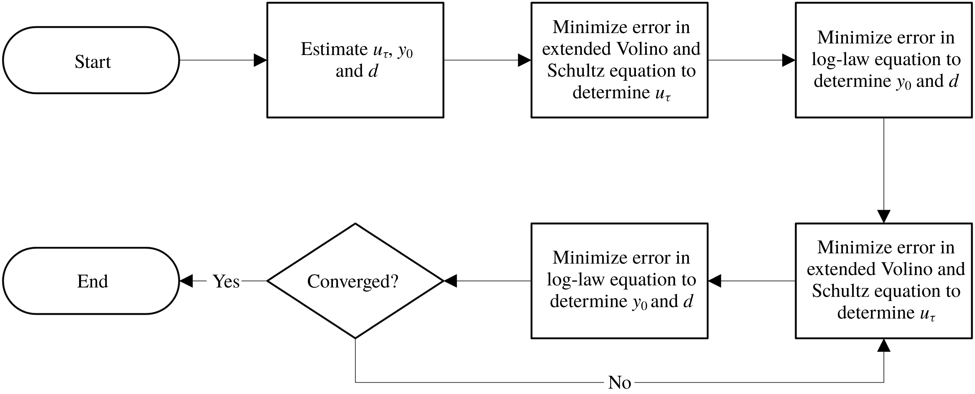
When friction velocity is initially unknown, it may be determined through (2.3) and (2.4) through an iterative method. The process is illustrated in a flowchart in figure 6. An initial estimate of the friction velocity, roughness length and zero-plane displacement is required since both equations have dependencies in all three variables. Then, (2.3) is used to determine
 $u_{\unicode[STIX]{x1D70F}}$
with the estimated
 $y_{0}$
and
 $d$
by minimizing the error in (2.3) (note that
 $u_{\unicode[STIX]{x1D70F}}$
enters in all of the terms) as explained in more detail when presenting applications below. Equation (2.3) is not highly sensitive to errors in
 $y_{0}$
and
 $d$
, so determining
 $u_{\unicode[STIX]{x1D70F}}$
with this equation first is the best way to reduce error in the initial estimate. However, since
 $u_{\unicode[STIX]{x1D70F}}$
is determined only semi-independently from (2.3), iterations are required to refine the solution. Next, equation (2.4) is used to determine
 $y_{0}$
and
 $d$
with the calculated
 $u_{\unicode[STIX]{x1D70F}}$
from the previous step. Then, solution refinement proceeds iteratively between (2.3) and (2.4) until specified stopping criteria are met. The stopping criteria for the experimental data sets shown in § 3 were three significant digits for
 $u_{\unicode[STIX]{x1D70F}}$
and
 $y_{0}$
or 10 iterations. Most data sets converged within a few iterations.


3 Applications to experimental data sets
In this section the analysis of terms in the momentum balance equation (which was presented in the prior section and led to the iterative method to determine the friction velocity based on single-location mean velocity and Reynolds shear stress profiles) is used to determine boundary layer parameters for various experimental data sets. Where required,
 $\unicode[STIX]{x1D705}$
and
 $A$
were assumed to be
 $0.384$
and
 $4.17$
, respectively, throughout § 3. The resulting friction velocities are compared to direct measurements using force balances or to prior published values.
3.1 Boundary layers over rough sand-grain surfaces
The comprehensive shear stress boundary layer analysis method was applied to the sand-grain boundary layer data from Squire et al. (Reference Squire, Morrill-Winter, Hutchins, Schultz, Klewicki and Marusic2016). This study recorded detailed fluid profile statistics with a cross-wire anemometry probe at multiple Reynolds numbers. The study also utilized a drag balance for independently measuring friction velocity directly at three of the Reynolds numbers tested. The present method is used to analyse turbulent boundary layer data with only the fluid measurements and without the friction velocity data from the force balance at the three Reynolds numbers profiled above the drag balance location. Figure 7 shows the present method’s result for the sand-grain surface with
 $Re_{\unicode[STIX]{x1D70F}}=6770$
. Figure 7(a) shows the mean streamwise velocity profile versus wall-normal distance, and figure 7(b) shows the Reynolds shear stress data versus wall-normal distance, in inner and outer scaling, respectively. The outer-scaled wall-normal distance,
 $\unicode[STIX]{x1D713}$
, is calculated by
 $$\begin{eqnarray}\displaystyle \unicode[STIX]{x1D713}=\frac{y-d}{\unicode[STIX]{x1D6FF}-d}. & & \displaystyle\end{eqnarray}$$
Evidence from Volino & Schultz (Reference Volino and Schultz2018) showed that reasonable estimates of flow below the nearest velocity data to the wall can be used to improve results. The estimated velocities only affect the integral terms in (2.3). In the following results, a cubic interpolation is used to estimate mean streamwise velocity between the nearest data point and an assumed zero velocity at
 $y=d$
. Flow below
 $y=d$
is assumed to be a negligible portion of the integrals, which is consistent with evidence from Volino & Schultz (Reference Volino and Schultz2018). This is not proposed as a universal method for interpolation but works well for better estimating the integral terms of (2.3).
Comparison of data and fits from the proposed method for mean velocity (a) and shear stress (b) profiles from Squire et al. (Reference Squire, Morrill-Winter, Hutchins, Schultz, Klewicki and Marusic2016) at
 $Re_{\unicode[STIX]{x1D70F}}=6770$
. Blue circles (●) are measured data, and red diamonds (♦) are fitted data. Fit to (2.4) performed on data between
 $0.07<\unicode[STIX]{x1D713}_{(k)}<0.15$
, and fit to (2.3) performed on data between
 $0.05<\unicode[STIX]{x1D713}_{(k)}<0.30$
. Green lines show (2.4) in (a) and (2.3) in (b). Dotted or dashed line styles show components of (2.3): brown dash-dot line is
 $1-\text{I}$
, cyan dashed line is
 $1-\text{I}-\text{II}$
and magenta dotted line is
 $1-\text{I}-\text{II}+\text{III}$
.

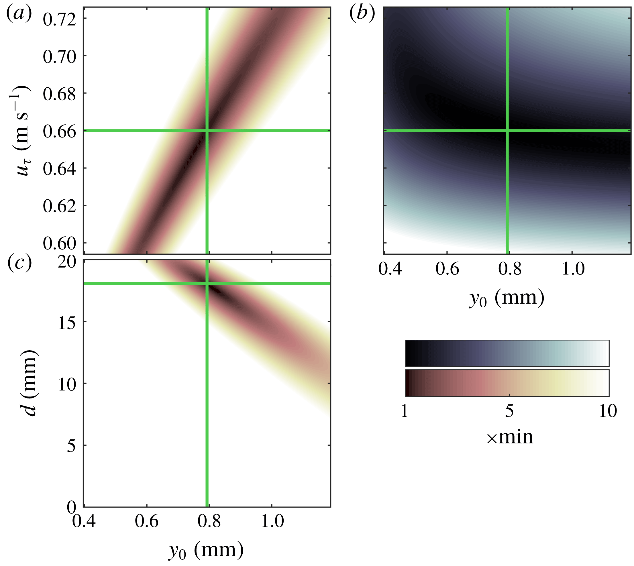
Contour plots of r.m.s. errors of fits to experimental data for boundary layer flow over sand-grain surface at
 $Re_{\unicode[STIX]{x1D70F}}=6770$
from Squire et al. (Reference Squire, Morrill-Winter, Hutchins, Schultz, Klewicki and Marusic2016). Panels (a,c) show the mean velocity r.m.s. errors between (2.4) and experimental data in the range
 $0.07<\unicode[STIX]{x1D713}_{(k)}<0.15$
calculated as shown in (3.3). Panel (b) shows the r.m.s. error between (2.3) and experimental data in the range
 $0.05<\unicode[STIX]{x1D713}_{(k)}<0.30$
calculated as shown in (3.2). The green lines show the converged values for
 $u_{\unicode[STIX]{x1D70F}}$
,
 $y_{0}$
and
 $d$
on the plots.

Having presented the results from the method as applied to the data, some details about the iterative procedure are presented next. Initial estimates for
 $u_{\unicode[STIX]{x1D70F}}$
,
 $y_{0}$
and
 $d$
may be used with (2.3) and (2.4) to start the iterative process shown in figure 6 for solving the unknowns. To illustrate the process, root mean square (r.m.s.) error plots in the variable parameter space are shown in figure 8. The r.m.s. error for (2.3) is calculated as usual according to
 $$\begin{eqnarray}\displaystyle \text{r.m.s. error}=\sqrt{\frac{1}{n}\mathop{\sum }_{k=1}^{n}[-\langle \overline{u^{\prime }v^{\prime }}\rangle _{(k)}^{+}-\langle \tilde{u} \tilde{v}\rangle _{(k)}^{+}-(1-\text{I}-\text{II}+\text{III}+\text{IV})_{(k)}]^{2}}, & & \displaystyle\end{eqnarray}$$
where the summation is over the
 $n$
experimental data points between
 $0.05<\unicode[STIX]{x1D713}_{(k)}<0.30$
. Figure 8(b) shows the r.m.s. error in the
 $u_{\unicode[STIX]{x1D70F}}{-}y_{0}$
plane and indicates that the r.m.s. error is much more sensitive to changes in
 $u_{\unicode[STIX]{x1D70F}}$
than changes in
 $y_{0}$
in the fitted region. The process of solving (2.3) for
 $u_{\unicode[STIX]{x1D70F}}$
effectively solves for the minimum on a vertical line of this plot since
 $y_{0}$
is assumed as given in this step of the process. This plot also helps illustrate that the error minimization from the comprehensive shear stress profile is well suited for solving
 $u_{\unicode[STIX]{x1D70F}}$
accurately.
Figure 8(a,c) shows r.m.s. error for (2.4) for the experimental data between
 $0.07<\unicode[STIX]{x1D713}_{(k)}<0.15$
calculated by
 $$\begin{eqnarray}\displaystyle \text{r.m.s. error}=\sqrt{\frac{1}{n}\mathop{\sum }_{k=1}^{n}\left[\frac{\langle U(y_{(k)})\rangle }{u_{\unicode[STIX]{x1D70F}}}-\frac{1}{\unicode[STIX]{x1D705}}\ln \left(\frac{y_{(k)}-d}{y_{0}}\right)\right]^{2}}. & & \displaystyle\end{eqnarray}$$
Figure 8(c) is the r.m.s. error in the
 $d-y_{0}$
plane which is the solution plane of interest for this step in the process. The range of
 $d$
on the vertical axis encompasses the total height of the sand-grain roughness from valleys to peaks. This is the total possible range for
 $d$
in accordance with the physical definition proposed by Jackson (Reference Jackson1981). The plot shows a strong dependence on
 $y_{0}$
but very weak dependence on
 $d$
in this range. For some experimental data sets including this case, a two-parameter fit of (2.4) can result in non-physical values of
 $d$
which should fall between the peaks and valleys of the roughness. Therefore, in some cases it may be more advantageous to assume a reasonable
 $d$
. For the case of figure 7 and the other two cases in table 1,
 $d$
was assumed to be the midpoint between peaks and valleys of the sand-grain surface as was assumed by Squire et al. (Reference Squire, Morrill-Winter, Hutchins, Schultz, Klewicki and Marusic2016) and Morrill-Winter et al. (Reference Morrill-Winter, Squire, Klewicki, Hutchins, Schultz and Marusic2017). Then a numerical solver was used to minimize (3.3) with
 $y_{0}$
only, which solves for the minimum error on a horizontal line of figure 8(c) rather than the absolute minimum error as a two-parameter fit would.
Iteration between solving (2.3) for
 $u_{\unicode[STIX]{x1D70F}}$
and solving (2.4) for
 $y_{0}$
converges to a unique solution because of the different sensitivities in the
 $u_{\unicode[STIX]{x1D70F}}{-}y_{0}$
plane shown in figure 8(a,b). Iteration progresses until the process converges to a unique solution. The green lines show the converged values for
 $u_{\unicode[STIX]{x1D70F}}$
,
 $y_{0}$
and
 $d$
for the case of figure 7.
Table 1 contains the three cases from Squire et al. (Reference Squire, Morrill-Winter, Hutchins, Schultz, Klewicki and Marusic2016) where fluid profiles were measured directly over the HRN-BLWT drag balance. Table 1 shows that the results from the present method of determining friction velocity agree with the direct drag balance measurements within
 $\pm 1\,\%$
. This agreement is well within the experimental uncertainties and shows the present method to be a reliable analysis technique when only fluid dynamic measurements are available at a single streamwise location.
Squire et al. (Reference Squire, Morrill-Winter, Hutchins, Schultz, Klewicki and Marusic2016) published drag balance friction velocity and the present method’s calculated friction velocity by fitting data between
 $0.05<\unicode[STIX]{x1D713}_{(k)}<0.30$
to (2.3) and fitting data between
 $0.07<\unicode[STIX]{x1D713}_{(k)}<0.15$
to (2.4).

3.2 Boundary layers over smooth walls
Next, the present method is applied to the smooth-wall fluid profile data from Morrill-Winter et al. (Reference Morrill-Winter, Klewicki, Baidya and Marusic2015). Determining
 $y_{0}$
and
 $d$
from the log-law equation, (2.4), in the flowchart of figure 6 is replaced with the explicit formula
 $y_{0}(u_{\unicode[STIX]{x1D70F}})=(\unicode[STIX]{x1D708}/u_{\unicode[STIX]{x1D70F}})\text{e}^{-\unicode[STIX]{x1D705}A}$
and with
 $d=0$
as described in § 2.2. Figure 9 shows fits of (2.3) and (2.4) for the smooth-wall ZPG flow at
 $Re_{\unicode[STIX]{x1D70F}}=1951$
.
Table 2 shows friction velocity results for a range of Reynolds numbers from the HRN-BLWT smooth-wall cases. The present method calculates
 $u_{\unicode[STIX]{x1D70F}}$
within
 $\pm 1\,\%$
of the published values from a single profile of fluid dynamic measurements for all cases analysed. While this study did not utilize a drag balance for friction velocity, Morrill-Winter et al. (Reference Morrill-Winter, Klewicki, Baidya and Marusic2015) used the composite fit method from Chauhan, Monkewitz & Nagib (Reference Chauhan, Monkewitz and Nagib2009) which has been validated extensively. The very good agreement of results in figure 9 and table 2 again show the present method to be a very accurate analysis technique and the indirect methods for calculating streamwise gradients in (2.3) to be reliable.
Comparison of data and fits from the proposed method for mean velocity (a) and shear stress (b) profiles from Morrill-Winter et al. (Reference Morrill-Winter, Klewicki, Baidya and Marusic2015) at
 $Re_{\unicode[STIX]{x1D70F}}=1951$
. Blue circles (●) are measured data, and red diamonds (♦) are fitted data. Fit to (2.4) performed on data between
 $0.07<y_{(k)}/\unicode[STIX]{x1D6FF}<0.15$
, and fit to (2.3) performed on data between
 $0.05<y_{(k)}/\unicode[STIX]{x1D6FF}<0.30$
. Green lines show (2.4) in (a) and (2.3) in (b). Dotted or dashed line styles show components of (2.3): brown dash-dot line is
 $1-\text{I}$
, cyan dashed line is
 $1-\text{I}-\text{II}$
and magenta dotted line is
 $1-\text{I}-\text{II}+\text{III}$
.

Morrill-Winter et al. (Reference Morrill-Winter, Klewicki, Baidya and Marusic2015) published friction velocities and the present method’s calculated friction velocities by fitting data between
 $0.05<y_{(k)}/\unicode[STIX]{x1D6FF}<0.30$
to (2.3) and fitting data between
 $0.07<y_{(k)}/\unicode[STIX]{x1D6FF}<0.15$
to (2.4).

3.3 Boundary layers over arrays of wall attached staggered cubes
The present method is also demonstrated for boundary layer data from Cheng & Castro (Reference Cheng and Castro2002) for flow over an array of wall attached cubes. Cross-wire anemometry profiles were recorded at multiple locations over a repeating unit for five different cases. Spatially averaged profiles from the
 $20~\text{mm}$
staggered cube array with 25 % planform surface density are shown here in figure 10 with fits from (2.3) and (2.4). Since the profiles shown are spatially averaged, the dispersive shear stress term is non-zero and included although it is small enough to be considered negligible. The r.m.s. error plots for these fits are shown in figure 11. Equation (2.4) is fit for data between
 $0<\unicode[STIX]{x1D713}_{(k)}<0.22$
which is equivalent to the published range used for this fit by Cheng & Castro (Reference Cheng and Castro2002). Equation (2.3) was fit between
 $0.15<\unicode[STIX]{x1D713}_{(k)}<0.30$
. Additionally, this test case had a single
 $20~\text{mm}$
brass cube which was instrumented with 21 pressure taps on the windward and leeward sides of the cube to directly measure pressure drag. In the fully rough regime, the pressure drag is very nearly the total surface drag. The same geometry was also tested in Cheng et al. (Reference Cheng, Hayden, Robins and Castro2007) with both the pressure-tapped cube and a floating element drag balance which will allow additional comparison for the friction velocity results.
Comparison of data and fits from the proposed method for mean velocity (a) and shear stress (b) profiles from Cheng & Castro (Reference Cheng and Castro2002) for flow over staggered
 $20~\text{mm}$
cubes. Blue circles (●) are measured data, and red diamonds (♦) are fitted data. Fit to (2.4) performed on data between
 $0<\unicode[STIX]{x1D713}_{(k)}<0.22$
, and fit to (2.3) performed on data between
 $0.15<\unicode[STIX]{x1D713}_{(k)}<0.30$
. Green lines show (2.4) in (a) and (2.3) in (b). Dotted or dashed line styles show components of (2.3): brown dash-dot line is
 $1-\text{I}$
, cyan dashed line is
 $1-\text{I}-\text{II}$
and magenta dotted line is
 $1-\text{I}-\text{II}+\text{III}$
.

Contour plots of r.m.s. errors of fits to experimental data for boundary layer flow over staggered cubes from Cheng & Castro (Reference Cheng and Castro2002). Panels (a,c) show the mean velocity r.m.s. errors between (2.4) and experimental data in the range
 $0<\unicode[STIX]{x1D713}_{(k)}<0.22$
calculated as shown in (3.3). Panel (b) shows the r.m.s. error between (2.3) and experimental data in the range
 $0.15<\unicode[STIX]{x1D713}_{(k)}<0.30$
calculated as shown in (3.2). The green lines show the converged values for
 $u_{\unicode[STIX]{x1D70F}}$
,
 $y_{0}$
and
 $d$
on the plots.
Differences between published friction velocities and the present method’s calculated friction velocity assuming ZPG. Hot-wire profiles for the present method were from Cheng & Castro (Reference Cheng and Castro2002). Published friction velocities are from Cheng et al. (Reference Cheng, Hayden, Robins and Castro2007).

As is evident from the results in table 3, the present comprehensive shear stress method does not seem any better than earlier approaches. The difference between the present method and the direct measures is still approximately
 $8\,\%{-}11\,\%$
. Additionally, even though (2.3) seems to fit the shear stress data below
 $\unicode[STIX]{x1D713}<0.5$
in figure 10(b), there are visual discrepancies in the slope particularly in the near-wall region,
 $\unicode[STIX]{x1D713}<0.25$
, where the equation should be the most accurate (due to less experimental error in the integral terms). This difference tends to lower the fitted value of friction velocity in agreement with other fluids based methods and no closer to the direct measurements.
The key problem with the results in table 3 is the discrepancy between the direct measurement methods and total shear stress methods (including the present method as applied above). In study after study, the traditional total shear stress methods seem to under-predict the friction velocity which has resulted in considerable discussion in the literature, such as in Cheng et al. (Reference Cheng, Hayden, Robins and Castro2007), Claus, Krogstad & Castro (Reference Claus, Krogstad and Castro2012) and Ferreira et al. (Reference Ferreira, Rodriguez-Lopez and Ganapathisubramani2018). The discussions persist to this date because, to the authors’ knowledge, this empirical discrepancy has not been quantified by physical equations. Additionally, studies by Reynolds & Castro (Reference Reynolds and Castro2008) and Placidi & Ganapathisubramani (Reference Placidi and Ganapathisubramani2015) both cite Cheng & Castro (Reference Cheng and Castro2002) and Cheng et al. (Reference Cheng, Hayden, Robins and Castro2007) for evidence-based corrections to the friction velocity which they determine from traditional total shear stress methods.
One of the possibilities noted by Cheng et al. (Reference Cheng, Hayden, Robins and Castro2007) and Ferreira et al. (Reference Ferreira, Rodriguez-Lopez and Ganapathisubramani2018) is that a small favourable pressure gradient (FPG) may cause this effect on the Reynolds shear stress. The University of Surrey and University of Southampton tunnels where these studies were conducted are considered nominally zero pressure gradient. However, both tunnels have a fixed cross-sectional area which imposes a small favourable pressure gradient due to boundary layer growth. From reported boundary layer growth in Cheng et al. (Reference Cheng, Hayden, Robins and Castro2007) and the tunnel dimensions, it can be estimated that the acceleration parameter was approximately
 $K=2\times 10^{-8}$
. This acceleration parameter is small (but non-zero) and in the range of values from the similarly sized fixed cross-section tunnel in Placidi & Ganapathisubramani (Reference Placidi and Ganapathisubramani2019).
Therefore, in evaluating term IV,
 $\text{d}\unicode[STIX]{x1D703}/\text{d}x$
may be replaced with the full MIE shown by
 $$\begin{eqnarray}\displaystyle \frac{\text{d}\unicode[STIX]{x1D703}}{\text{d}x}=\frac{c_{f}}{2}-\left(\frac{2\unicode[STIX]{x1D703}}{\unicode[STIX]{x1D6FF}}+\frac{\unicode[STIX]{x1D6FF}^{\ast }}{\unicode[STIX]{x1D6FF}}\right)\left(\frac{U_{e}\unicode[STIX]{x1D6FF}}{\unicode[STIX]{x1D708}}\right)K & & \displaystyle\end{eqnarray}$$
to solve
 $\unicode[STIX]{x2202}\langle U\rangle ^{+}/\unicode[STIX]{x2202}x|_{y^{+}}$
from (2.17). Also, for term III of (2.3), equation (2.13) may still be used to solve
 $(\text{d}/\text{d}x)\sqrt{c_{f}/2}$
. The evidence from Castro (Reference Castro2007) indicates that (2.13) still holds for small FPG boundary layers. Castro (Reference Castro2007) shows a plot of
 $c_{f}$
versus
 $(x-x_{0})/y_{0}$
. Equation (2.13) is derived from the curve in Castro’s plot, and most (if not all) of the experimental data on the plot are from fixed cross-section tunnels with small FPGs.
Figure 12 shows Cheng & Castro (Reference Cheng and Castro2002) cross-wire anemometry data with fits from (2.3) and (2.4) using the present method. Equation (2.3) is now calculated for a small FPG which assumes
 $K=2\times 10^{-8}$
. Equation (2.3) now agrees with the turbulent shear stress data well through
 $\unicode[STIX]{x1D713}<0.4$
. Furthermore, it matches the slope below
 $\unicode[STIX]{x1D713}<0.25$
where it had not previously. Comparing figures 10(b) and 12(b), the effect on the terms of (2.3) is readily seen. Term II, a purely pressure dependent term, was zero in figure 10 but approximately half of the total shear stress throughout the boundary layer in figure 12. Additionally, the magnitude of both terms III and IV were reduced due to the positive
 $K$
in term III and (3.4). The overall effect from the pressure gradient flattened the turbulent shear stress profile throughout the boundary layer by reducing the inertial terms and increasing the pressure-dependent terms.
Comparison of data and fits from the proposed method for mean velocity (a) and shear stress (b) profiles from Cheng & Castro (Reference Cheng and Castro2002) for flow over staggered
 $20~\text{mm}$
cubes. Blue circles (●) are measured data, and red diamonds (♦) are fitted data. Fit to (2.4) performed on data between
 $0<\unicode[STIX]{x1D713}_{(k)}<0.22$
, and fit to (2.3) performed on data between
 $0.15<\unicode[STIX]{x1D713}_{(k)}<0.30$
. Green lines show (2.4) in (a) and (2.3) in (b). Dotted or dashed line styles show components of (2.3): brown dash-dot line is
 $1-\text{I}$
, cyan dashed line is
 $1-\text{I}-\text{II}$
and magenta dotted line is
 $1-\text{I}-\text{II}+\text{III}$
. Equation (2.3) is calculated assuming a small FPG with
 $K=2\times 10^{-8}$
.

Differences between published friction velocities and the present method’s calculated friction velocity assuming small FPG with
 $K=2\times 10^{-8}$
. Hot-wire profiles for the present method were from Cheng & Castro (Reference Cheng and Castro2002). Published friction velocities are from Cheng et al. (Reference Cheng, Hayden, Robins and Castro2007).

Table 4 compares results from the present method now assuming a small favourable pressure gradient. The present result is now 7 % lower than the pressure-tapped cube and 6 % lower than the floating element drag balance. This is encouraging because the comprehensive shear stress method is now within the 10 % published uncertainty of the pressure-tapped cube measurements in Cheng et al. (Reference Cheng, Hayden, Robins and Castro2007). The floating element drag balance does not appear to have published information regarding experimental uncertainty. It may be assumed that the uncertainty is at least 3 % which would be in line with other floating element drag balances used in a similar tunnel by Placidi & Ganapathisubramani (Reference Placidi and Ganapathisubramani2015) and Ferreira et al. (Reference Ferreira, Rodriguez-Lopez and Ganapathisubramani2018). Additionally, the uncertainty in the present method is unknown especially given that
 $K$
was estimated with limited information. Given these uncertainties the present method appears to be an improvement to prior single fluid profile measurement approaches.
Comparison of data and fits from the proposed method for mean velocity (a) and shear stress (b) profiles from Placidi & Ganapathisubramani (Reference Placidi and Ganapathisubramani2015) LEGO® block geometry LP2 at
 $Re_{\unicode[STIX]{x1D70F}}=7642$
. Blue circles (●) are measured data, and red diamonds (♦) are fitted data. Some data points were removed for clarity. Fit to (2.4) performed on data between
 $0.07<\unicode[STIX]{x1D713}_{(k)}<0.15$
, and fit to (2.3) performed on data between
 $0.15<\unicode[STIX]{x1D713}_{(k)}<0.30$
. Green lines show (2.4) in (a) and (2.3) in (b). Dotted or dashed line styles show components of (2.3): brown dash-dot line is
 $1-\text{I}$
, cyan dashed line is
 $1-\text{I}-\text{II}$
and magenta dotted line is
 $1-\text{I}-\text{II}+\text{III}$
. Equation (2.3) is calculated with
 $K$
from table 5.

3.4 Boundary layers over arrays of LEGO® blocks
Placidi & Ganapathisubramani (Reference Placidi and Ganapathisubramani2015, Reference Placidi and Ganapathisubramani2018) tested 12 fully rough surfaces with different repeating patterns of LEGO® blocks. The studies were nominally zero pressure gradient and reported that
 $K<5\times 10^{-8}$
. The authors published the data set online in Placidi & Ganapathisubramani (Reference Placidi and Ganapathisubramani2019) which included calculated pressure gradients. The study published
 $u_{\unicode[STIX]{x1D70F}}$
values from direct measurement with a force balance, and
 $y_{0}$
and
 $d$
were found with a least square regression of the log-law equation using the friction velocity measured from the force balance. The drag balance in this study was based on the design documented in Krogstad & Efros (Reference Krogstad and Efros2010) and is expected to be more accurate than the one in Cheng et al. (Reference Cheng, Hayden, Robins and Castro2007).
Turbulent boundary layer data plotted in figure 13 were recorded by particle image velocimetry over the surface geometry named LP2 at
 $Re_{\unicode[STIX]{x1D70F}}=7642$
. Figure 13 shows fits to the particle image velocimetry data for (2.3) and (2.4). Placidi & Ganapathisubramani (Reference Placidi and Ganapathisubramani2019) published
 $K=4.3\times 10^{-8}$
for this case. Equation (2.4) was fitted to velocity data between
 $0.07<\unicode[STIX]{x1D713}_{(k)}<0.15$
in figure 13(a), and (2.3) was fitted to shear stress data between
 $0.15<\unicode[STIX]{x1D713}_{(k)}<0.30$
in figure 13(b).
All six surfaces from Placidi & Ganapathisubramani (Reference Placidi and Ganapathisubramani2015) with constant frontal density (LP1–LP6) were analysed with the present method assuming both a ZPG and a small FPG. In some cases, it was necessary to fix the range of possible
 $d$
to within the roughness height due to the physical interpretation of
 $d$
described in Jackson (Reference Jackson1981). Placidi & Ganapathisubramani (Reference Placidi and Ganapathisubramani2015) also noted this was necessary for some cases in their analysis. Results are included in table 5. The present method’s result was consistently lower than the drag balance measurement when a ZPG was assumed but was close to the experimental uncertainty of the drag balance for five of the six cases when the reported
 $K$
(for the small FPG) was utilized. Case LP6, which differed by
 $-18\,\%$
or
 $-17\,\%$
, remains as an outlier for which the present fluid dynamic measurements alone do not agree with the drag balance measurement.
Differences between Placidi & Ganapathisubramani (Reference Placidi and Ganapathisubramani2015) published drag balance friction velocity and the present method’s calculated friction velocities by fitting data between
 $0.15<\unicode[STIX]{x1D713}_{(k)}<0.30$
to (2.3) and fitting data between
 $0.07<\unicode[STIX]{x1D713}_{(k)}<0.15$
to (2.4). Acceleration parameters,
 $K$
, obtained from Placidi & Ganapathisubramani (Reference Placidi and Ganapathisubramani2019).

Placidi & Ganapathisubramani (Reference Placidi and Ganapathisubramani2015) reported that it was necessary to increase
 $u_{\unicode[STIX]{x1D70F}}$
determined from traditional total shear stress methods by
 $12\,\%$
in order to obtain agreement within 5 % of the drag balance results for all cases. The present method does not need a correction factor and achieves considerably better results both assuming a ZPG and small FPG. Utilizing the reported
 $K$
for the small FPG leads to results that are near the uncertainty of the study’s drag balance in a tunnel similar to the one in Cheng & Castro (Reference Cheng and Castro2002). These results give strong evidence that the small FPG explains the often cited friction velocity discrepancy from Cheng & Castro (Reference Cheng and Castro2002).
3.5 Friction velocity sensitivity
The comprehensive shear stress method assumes
 $\unicode[STIX]{x1D705}$
, the fitting range for the extended Volino & Schultz equation, (2.3), and the fitting range for the log-law equation, (2.4), when solving for
 $u_{\unicode[STIX]{x1D70F}}$
,
 $y_{0}$
and
 $d$
. A trivariate sensitivity analysis was performed on surface geometry LP2 from Placidi & Ganapathisubramani (Reference Placidi and Ganapathisubramani2015). Converged values of
 $u_{\unicode[STIX]{x1D70F}}$
,
 $y_{0}$
and
 $d$
were calculated for all 150 combinations of
 $\unicode[STIX]{x1D705}$
, fitting range to (2.3), and fitting range to (2.4) from table 6. Figure 15 shows scatter plots of the results projected onto the three planes created by
 $u_{\unicode[STIX]{x1D70F}}$
,
 $y_{0}$
, and
 $d$
. Friction velocity results show low sensitivity to the assumed parameters with
 $u_{\unicode[STIX]{x1D70F}}$
bounded within
 $\pm 2\,\%$
of the results from § 3.4.
While friction velocity showed low sensitivity, results for
 $y_{0}$
ranged from 38 % below to 5 % above the results from § 3.4. Also, results for
 $d$
included nearly the entire upper
 $1/3$
of the roughness height. The variances in
 $y_{0}$
and
 $d$
were primarily from the high sensitivity inherent in fitting the log-law equation, equation (2.4). The present method shares this limitation with other methods that rely on two-parameter fits to the log-law equation. However, the selected log-law fitting range does not greatly affect the friction velocity result.
Contour plots of r.m.s. errors of fits to experimental data for boundary layer flow from Placidi & Ganapathisubramani (Reference Placidi and Ganapathisubramani2015) LEGO® block geometry LP2. Panels (a,c) show the mean velocity r.m.s. errors between (2.4) and experimental data in the range
 $0.07<\unicode[STIX]{x1D713}_{(k)}<0.15$
calculated as shown in (3.3). Panel (b) shows the r.m.s. error between (2.3) and experimental data in the range
 $0.15<\unicode[STIX]{x1D713}_{(k)}<0.30$
calculated as shown in (3.2). The green lines show the converged values for
 $u_{\unicode[STIX]{x1D70F}}$
,
 $y_{0}$
and
 $d$
on the plots.

Scatter plots showing
 $u_{\unicode[STIX]{x1D70F}}$
,
 $y_{0}$
and
 $d$
trivariate sensitivity to assumptions of
 $\unicode[STIX]{x1D705}$
, fitting range for (2.3), and fitting range for (2.4) applied to data from Placidi & Ganapathisubramani (Reference Placidi and Ganapathisubramani2015) LEGO® block geometry LP2. The solid green lines show the converged values plotted in figure 14. The dashed green lines show
 $u_{\unicode[STIX]{x1D70F}}\pm 2\,\%$
.

Parameter variations for univariate and trivariate sensitivity analysis for Placidi & Ganapathisubramani (Reference Placidi and Ganapathisubramani2015). Bracketed parameters indicate the initial assumptions from § 3.4.

A univariate analysis was also performed for all cases with constant frontal density from Placidi & Ganapathisubramani (Reference Placidi and Ganapathisubramani2015) excluding the outlier, LP6. In each plot of figure 16, one of the three assumed parameters was allowed to vary with the values listed in table 6 while maintaining the initial assumptions from § 3.4 in the other two parameters. The varying parameter is labelled on the horizontal axis with the vertical axis showing the maximum positive and negative per cent difference to the
 $u_{\unicode[STIX]{x1D70F}}$
reported in table 5 for each case. The figure shows that each of the three assumptions individually affect the friction velocity result by less than
 $\pm 1\,\%$
.
Bar plots showing univariate sensitivity of
 $u_{\unicode[STIX]{x1D70F}}$
to assumptions of
 $\unicode[STIX]{x1D705}$
, fitting range for (2.3), and fitting range for (2.4) applied to data from Placidi & Ganapathisubramani (Reference Placidi and Ganapathisubramani2015). Per cent sensitivity bars show the maximum positive and negative per cent differences to the
 $u_{\unicode[STIX]{x1D70F}}$
reported in table 5 for each case.

4 Summary
4.1 Key assumptions
Several key assumptions were included in the derivation and application of the present method and are reviewed here. First, simplification of the integral form of the Reynolds-averaged and spatially averaged streamwise momentum equation assumed that Reynolds normal stresses were negligible and the flow was two-dimensional. Second, the derivation assumed that the skin friction law, equation (2.10), was applicable. There were several assumptions embedded in the skin friction law which were discussed in § 2.1.1, but the skin friction law was shown to have robust applicability both in § 2.1.1 and Castro (Reference Castro2007). Third, the friction velocity gradient equation, (2.13), used the ZPG MIE. However, it was noted that Castro (Reference Castro2007) applied the ZPG MIE to nominally ZPG boundary layers with good agreement. Also, results from § 3 imply that this was a valid assumption for
 $K\lesssim 5\times 10^{-8}$
. Fourth, the velocity gradient profile derivation assumed that velocity profiles would collapse in outer scaling over a streamwise distance. This condition implies that
 $\unicode[STIX]{x2202}\unicode[STIX]{x1D6F1}/\unicode[STIX]{x2202}x\approx 0$
,
 $W$
scales with
 $\unicode[STIX]{x1D6FF}$
and
 $\unicode[STIX]{x2202}\unicode[STIX]{x1D6FF}/\unicode[STIX]{x2202}\unicode[STIX]{x1D703}\approx \unicode[STIX]{x1D6FF}/\unicode[STIX]{x1D703}$
and is also sensitive to pressure gradient (and probably other parameters). However, the velocity gradient profile only appears in term IV of (2.3) which was not significant for
 $\unicode[STIX]{x1D713}<0.3$
in most cases. Thus, it can be more easily avoided by choosing an appropriate fitting range.
Friction velocities determined using different total shear stress (TSS) approaches, plotted against published friction velocities. Filled red symbols utilize the present comprehensive shear stress method. Open blue symbols utilize total shear stress points in the plateau region. Open green symbols utilize total shear stress points in the roughness sublayer and inertial sublayer (RS+IS). Open grey symbols utilize the peak total shear stress. Up triangle (▴) data are from Squire et al. (Reference Squire, Morrill-Winter, Hutchins, Schultz, Klewicki and Marusic2016). Down triangle (▾) data are from Morrill-Winter et al. (Reference Morrill-Winter, Klewicki, Baidya and Marusic2015). Right triangle (▸) data are from Placidi & Ganapathisubramani (Reference Placidi and Ganapathisubramani2015).

4.2 Results and comparisons with other methods
Figure 17 compares published measured friction velocity for rough-wall cases and the published composite fit friction velocity for smooth cases to traditional total shear stress methods and to the present method. Red points for the present method fall close to the
 $45^{\circ }$
line indicating excellent agreement with the published friction velocities. The one outlier is from surface LP6 from Placidi & Ganapathisubramani (Reference Placidi and Ganapathisubramani2015) as discussed in § 3.4. It is noted that no other method provided results within 11 % of the measured friction velocity for this case. Other approaches are shown on the figure with blue, green and grey open symbols, showing larger scatter and a downward bias. The dotted line shows the total shear stress friction velocity for which a 12 % correction would equal the drag balance friction velocity. It can be seen why it may be appropriate to utilize the 12 % empirical correction for some cases from Placidi & Ganapathisubramani (Reference Placidi and Ganapathisubramani2015) utilizing all total shear stress data from the roughness sublayer and inertial sublayer. However, other methods utilizing the plateau in the total shear stress and peak total shear stress provided results closer to the solid line. All total shear stress methods performed comparably for the smooth- and rough-wall cases from Morrill-Winter et al. (Reference Morrill-Winter, Klewicki, Baidya and Marusic2015) and Squire et al. (Reference Squire, Morrill-Winter, Hutchins, Schultz, Klewicki and Marusic2016), respectively.
Overall, no other total shear stress method performed as consistently well as the present method across all data sets considered. Besides one outlier, all cases utilizing the present method were within
 $\pm 4\,\%$
of the friction velocity measured with a drag balance.
5 Conclusions
A detailed analysis of several terms entering in the mean momentum balance of turbulent boundary layers was performed. The results were useful in formulating a new comprehensive shear stress method for determining friction velocity. The approach is based on measured profiles of mean velocity and turbulent shear stress at a single downstream location and can be used for analysing nominally zero pressure gradient turbulent boundary layers. The approach extends an equation from Volino & Schultz (Reference Volino and Schultz2018) to include spatial averaging and to calculate streamwise gradients from a single streamwise location. Two key elements are necessary to indirectly calculate streamwise gradients from a single two-component velocity profile. The first key element is the replacement of the streamwise gradient of friction velocity with an assumption of the skin friction law and momentum integral equation. The second key element is the assumption that the wake function scales with boundary layer thickness and can be connected to the streamwise gradient through the momentum integral equation. Application of the extended Volino & Schultz equation to various data sets showed the equation models turbulent shear stress data throughout the boundary layer. An iterative procedure combining fitting of the extended Volino & Schultz equation to the turbulent shear stress profile and fitting of the log-law equation to the mean velocity profile was proposed and implemented. Applications to various flows illustrated that the proposed method achieves similar friction velocity results as force balance measurements but only requires mean velocity and turbulent shear stress profiles. Results also demonstrated that even small pressure gradients, which can arise in fixed cross-section facilities, can have a significant (and often neglected) effect on turbulent shear stresses and may account for 10 % or more in friction velocity discrepancy with force balance measurements. The comprehensive shear stress method presented can account for this discrepancy in nominally zero pressure gradient facilities, leading to improved accuracy when determining friction velocity and skin friction drag in boundary layer experiments with commonly available profile data.
An interactive graphical user interface (GUI) software is available for download as part of the supplementary materials provided at http://pages.jh.edu/∼cmeneve1/datasets.html.
Acknowledgements
The authors would like to thank Dr D. Squire for providing the tabulated data published in Morrill-Winter et al. (Reference Morrill-Winter, Klewicki, Baidya and Marusic2015), Squire et al. (Reference Squire, Morrill-Winter, Hutchins, Schultz, Klewicki and Marusic2016) and Morrill-Winter et al. (Reference Morrill-Winter, Squire, Klewicki, Hutchins, Schultz and Marusic2017), and Professor I. Castro for providing tabulated data published in Cheng & Castro (Reference Cheng and Castro2002). Tabulated DNS data from Sillero et al. (Reference Sillero, Jiménez and Moser2013) were obtained from the website of the Fluid Dynamics Group of the Universidad Politécnica de Madrid. The authors would also like to thank Dr M. Placidi for providing the data published in Placidi & Ganapathisubramani (Reference Placidi and Ganapathisubramani2015, Reference Placidi and Ganapathisubramani2018, Reference Placidi and Ganapathisubramani2019) and for looking further into the experimental data to provide acceleration parameters at our request. We are also grateful to Professor R. Volino for insightful discussions, questions and recommendations that helped improve the paper. Finally, the authors gratefully acknowledge financial support from the National Defense Science and Engineering Graduate Fellowship (K.M.W.), the US Office of Naval Research (M.P.S.), and NSF grant CBET-1738918 (C.M.).