1. Introduction
Is economic growthFootnote 1 first dirty and then clean once countries become wealthier, as the environmental Kuznets curve (EKC) hypothesis proposes? Are higher emissions intensities associated with slower growth in emissions, or even reductions in emissions? How important are the time effects – changes in pollution not associated with economic growth – emphasized by Vollebergh et al. (Reference Vollebergh, Melenberg and Dijkgraaf2009)? The answers to these questions are not only important for understanding the relationship between economic growth and development theoretically, but also for projecting future business-as-usual emissions. In this paper, we present a new approach that combines the EKC model and beta convergence approaches to modeling the evolution of emissions in a single equation. This allows us to test the relative adequacy of these approaches as explanations of the evolution of emissions.
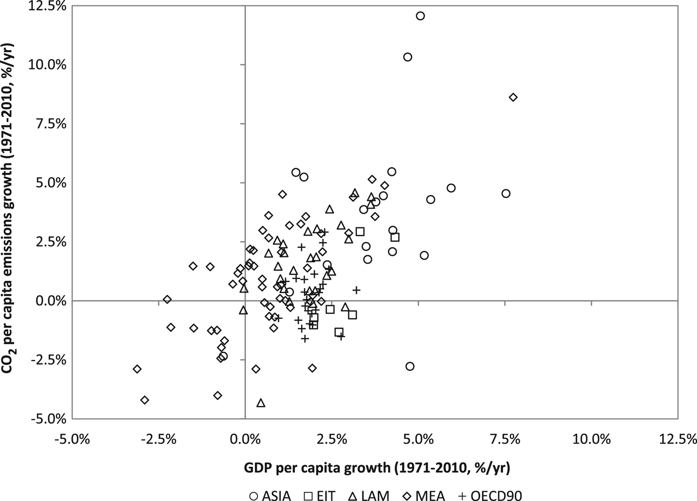
Our econometric approach is inspired by figure 1,Footnote 2 which shows a strong positive correlation between the long-run average growth rate of per capita carbon dioxide (CO2) emissions and the long-run average growth rate of GDP per capita. Fast-growing economies typically see increases in per capita CO2 emissions while slow-growing or declining economies tend to have declining per capita emissions. Figure 1 shows a fairly strong linear relationship between the rate of growth of per capita GDP and the rate of growth of per capita emissions, with the remaining variation reflecting differences in the rate of change in emissions per dollar of GDP (‘emissions intensity’). Emissions intensity declined in slightly more than half of the countries. Some rapidly growing economies, such as China, saw significant declines in emissions intensity, in many cases at a faster rate than in most developed countries.
Growth rates of per capita income and per capita carbon dioxide emissions from fossil fuel combustion and cement production

Figure 1 also shows that a number of slow-growing non-OECD countries have had declining per capita emissions, while some OECD countries have had rising per capita emissions. This suggests that a simple EKC story – that economic growth in poor countries increases per capita emissions while economic growth in rich countries reduces per capita emissions – cannot fully explain the data. The figure suggests a new and simple econometric approach: regressing the long-run average growth rate of per capita emissions on the long-run average growth rate of income per capita, and using additional variables to explain the remaining variation in emissions intensity.
In this paper, we assess the determinants of long-run per capita emissions growth rates using our new econometric approach, making two main contributions. First, our approach has important econometric advantages over the conventional panel data representation used to estimate EKC models. Secondly, our approach allows us to unify the main existing models – a simple IPAT model,Footnote 3 the EKC and the beta convergence approach – and directly test the relative explanatory power of each.
There are four econometric advantages of our long-run growth rates approach. First, we circumvent the unit root problem raised by Wagner (Reference Wagner2008), as unit roots are differenced. Secondly, by taking average growth rates over a long period of time, we filter out short-run effects and put more weight on the long-run components of variability.Footnote 4 Thirdly, we address the identification of time effects issue raised by Vollebergh et al. (Reference Vollebergh, Melenberg and Dijkgraaf2009); our model identifies the mean time effect as the mean long-run emissions growth rate when GDP growth is zero and other variables are at their sample mean. Fourthly, our approach reduces the main problem associated with the between estimator (BE) proposed by Stern (Reference Stern2010) – that omitted variables correlated with the levels of both emissions per capita and income per capita may result in biased estimates. In our new approach, the means of these variables are removed by differencing.
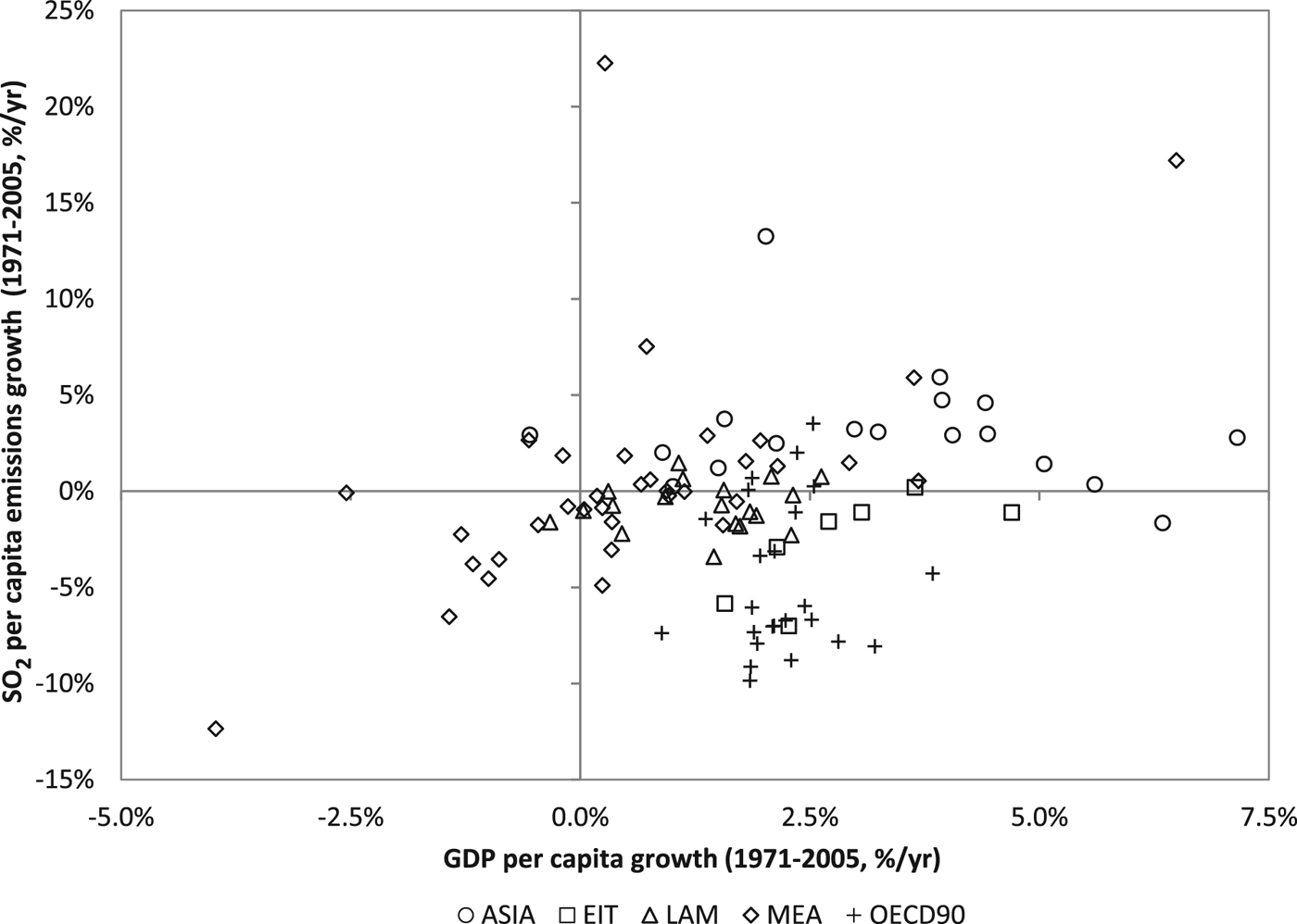
We estimate our model for CO2 emissions from fossil fuel combustion and cement production, as well as sulfur dioxide (SO2) emissions estimated by Smith et al. (Reference Smith, van Ardenne, Klimont, Andres, Volke and Arias2011). Long-run growth in SO2 emissions is again positively correlated with economic growth (figure 2), although the entire distribution of per capita emissions growth is shifted downwards, suggesting a strong negative time effect. There is a group of smaller OECD countries with very negative per capita emissions growth clustered toward the bottom of the figure.
Growth rates of per capita income and per capita sulfur dioxide emissions

Using our simple unified approach, we can reject the restrictions implied by models that exclude the initial levels of emissions and income. We can also easily reject the restrictions implied by Brock and Taylor's (Reference Brock and Taylor2010) short green Solow model, which excludes the growth rate of per capita GDP. Thus both growth and beta convergence effects are needed to explain emissions, as suggested by Ordás Criado et al. (Reference Ordás Criado, Valente and Stengos2011). For the full sample period, we do not find significant evidence in favor of the EKC hypothesis for either CO2 or SO2 emissions although the elasticity of per capita emissions growth with respect to per capita GDP growth – which we refer to as the ‘emissions–income elasticity’ – is lower in higher income countries. While we do find an in-sample income turning point for SO2 in the 1988–2005 period, this turning point is estimated imprecisely. Negative time effects are also important in explaining the reductions in per capita SO2 emissions experienced in some countries.
The outline of the paper is as follows. In section 2 we lay out prior work and in section 3 we present our research design. We then describe the overall features of the data in section 4, followed by results in section 5 and conclusions in section 6.
2. Prior research
There has been an extensive debate on the drivers of pollution emissions and other environmental impacts. Three main approaches have dominated the literature. Our method allows us to test all three in a single equation model.
Until the 1980s, mainstream environmental thought held that environmental impact increased with the scale of economic activity (i.e., aggregate GDP), although either more or less environmentally friendly technology could be chosen. This approach is represented by Ehrlich and Holdren's (Reference Ehrlich and Holdren1971) IPAT model. IPAT is an identity given by impact ≡ population * affluence * technology.Footnote 5 If affluence is taken to be income per capita, then the technology term is impact or emissions per dollar of income. If technology is independent of income per capita, then IPAT implies that the elasticity of per capita emissions with respect to per capita GDP (‘emissions–income elasticity’) is 1. We will use our long-run growth rates approach to test whether this is indeed the case.
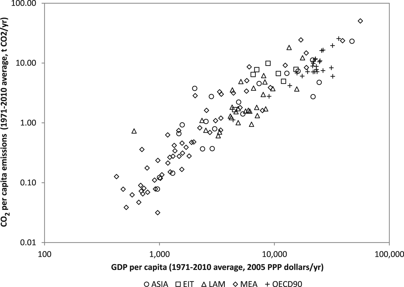
The 1980s saw the introduction of the sustainable development concept, which argued that development was not necessarily damaging to the environment and that poverty reduction was essential to protect the environment (WCED, 1987). In line with this idea, Grossman and Krueger (Reference Grossman and Krueger1991, Reference Grossman and Krueger1995) introduced the second main approach to modeling the income–emissions relationship – the EKC – which proposes that environmental impacts first increase and then decrease over the course of economic development.Footnote 6 Proponents of the EKC argue that, although economic growth at first increases environmental degradation, in the long run countries must become rich in order to clean up their environment (e.g., Beckerman, Reference Beckerman1992). The EKC was popularized by the 1992 World Development Report (World Bank, 1992), which relied on research by Shafik (Reference Shafik1994). However, this showed that per capita CO2 emissions do not seem to be an inverted U-shape function of GDP per capita, a conclusion also reached by Holtz-Eakin and Selden (Reference Holtz-Eakin and Selden1995). Figure 3 uses the same data featured in figure 1 to confirm the lack of a cross-country CO2 EKC.
Levels of per capita income and per capita carbon dioxide emissions from fossil fuel combustion and cement productio

Stern and Common (Reference Stern and Common2001) found that in a globally representative sample of countries, even for SO2 emissions, there was a monotonic relationship between per capita emissions and income per capita when time effects were included in the regression model. Recent papers using more sophisticated econometrics also find that the relationship between the levels of per capita emissions and income per capita is monotonic when the effect of the passage of time is controlled for (Wagner, Reference Wagner2008; Vollebergh et al., Reference Vollebergh, Melenberg and Dijkgraaf2009; Stern, Reference Stern2010). On the other hand, using a set of simple cross-sectional CO2 EKC regressions, Chow and Li (Reference Chow and Li2014) find a highly significant coefficient on the square of the log of GDP per capita (t=−22.9), claiming conclusive econometric evidence in favor of the CO2 EKC. However, their mean turning point is in fact at a GDP per capita level of US$378,000, so this result also supports a monotonic emissions–income trajectory.
Using Bayesian shrinkage estimators, Mazzanti and Musolesi, (Reference Mazzanti and Musolesi2013) find an in-sample turning point for per capita CO2 emissions for Northern European members of the EU but not for other developed countries. Their models do not allow for a time effect and they also removed Austria, Ireland and Norway, where emissions have not fallen, from the sample of Northern European countries. Non-parametric approaches have also been used to estimate the EKC (e.g., Carson et al., Reference Carson, Jeon and McCubbin1997; Millimet et al., Reference Millimet, List and Stengos2003; Azomahou et al., Reference Azomahou, Laisney and Nguyen-Van2006; Tsurumi and Managi, Reference Tsurumi, Managi and Managi2015), although many of these estimates also suffer from the issues raised by Wagner (Reference Wagner2008, Reference Wagner2015), Vollebergh et al. (Reference Vollebergh, Melenberg and Dijkgraaf2009) and others. These mostly do not produce radically different results from parametric estimates.
Even if the relationship between GDP per capita and per capita emissions is monotonic, an EKC-like pattern could emerge from a combination of growth and time effects (Stern, Reference Stern2004). Growth of per capita emissions in faster growing countries might outpace the efficiency improvements that come with time, so that per capita emissions would rise in fast-growing countries and decline in slow-growing countries. The fastest growing economies have been middle-income countries such as China and the Asian tiger economies that are catching up to the developed countries by adopting existing technologies.
The third main approach to the evolution of per capita emissions is to hypothesize that they are converging. There are three main approaches to testing for convergence: sigma convergence, which tests whether the dispersion of the variable in question declines over time using either just the variance or the full distribution (e.g., Ezcurra, Reference Ezcurra2007); stochastic convergence, which tests whether the time series for different countries cointegrate; and beta convergence, which tests whether the growth rate of a variable is negatively correlated to the initial level. Pettersson et al. (Reference Pettersson, Maddison, Acar and Söderholm2013) provide a review of the literature on convergence of per capita CO2 emissions.
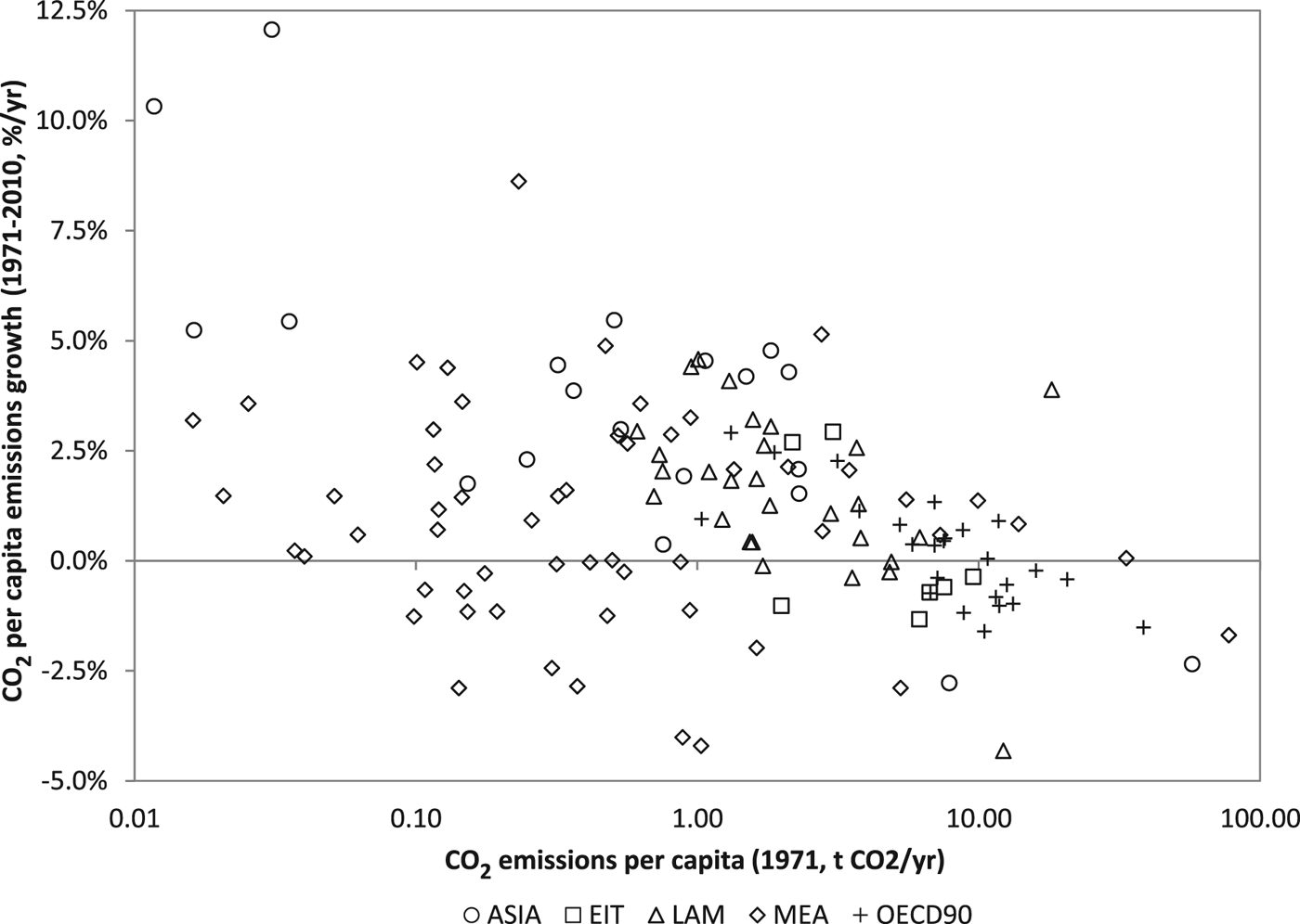
Using beta and stochastic convergence tests, Strazicich and List (Reference Strazicich and List2003) found convergence among developed economies. Using sigma convergence approaches, Aldy (Reference Aldy2006) found convergence for the developed economies but not the world as a whole. Using stochastic convergence, Westerlund and Basher (Reference Westerlund and Basher2008) reported convergence for a panel of 28 developed and developing countries over a very long period. Recent research using stochastic convergence finds evidence of club convergence rather than global convergence, however (Herrerias, Reference Herrerias2013; Pettersson et al., Reference Pettersson, Maddison, Acar and Söderholm2013). On the other hand, using the beta convergence approach, Brock and Taylor (Reference Brock and Taylor2010) found convergence among 165 developed and developing countries between 1960 and 1998. Figure 4 shows beta convergence for per capita CO2 emissions for our sample of countries. There is a clear tendency for emissions to grow in countries with a low initial level of emissions and vice versa.
Convergence in per capita carbon dioxide emissions from fossil fuel combustion and cement production

The beta convergence approach has been criticized (e.g., Quah, Reference Quah1993; Evans, Reference Evans1996; Evans and Karras, Reference Evans and Karras1996) because it is clear that dependence of the growth rate on the initial level of the variable is insufficient, though necessary (Pettersson et al., Reference Pettersson, Maddison, Acar and Söderholm2013), for actual sigma convergence. Beta convergence could also be purely due to regression to the mean (Friedman, Reference Friedman1992; Quah, Reference Quah1993). However, we find it hard to believe that, for example, the high levels of emissions intensity in formerly centrally planned economies are simply random fluctuations. In any case, economic theory – including Brock and Taylor's (Reference Brock and Taylor2010) green Solow model and Ordás Criado et al.'s (2011) model – suggests that the initial level of emissions should be a factor in explaining emissions growth. We are not, therefore, so concerned with whether countries’ emissions or emissions intensity actually converges in the sigma sense but whether the initial level of emissions or emissions intensity has an effect on future emissions growth.
Brock and Taylor's (Reference Brock and Taylor2010) theoretical green Solow model is essentially the IPAT decomposition with the addition of economic models to explain A and T (and the treatment of population as exogenous). They explain affluence or income per capita using the Solow (Reference Solow1956) growth model, in which poorer countries grow faster than rich countries. In Brock and Taylor's empirical analysis, they assume a constant rate of technological progress in pollution ‘abatement’ that is common across countries.Footnote 7 As a result, the growth rate of emissions is a function of initial emissions per capita and there is convergence in emissions per capita across countries over time. Depending on the specification chosen, this model explains 14–42 per cent of the variance in average national 1960–1998 per capita CO2 emissions growth rates.
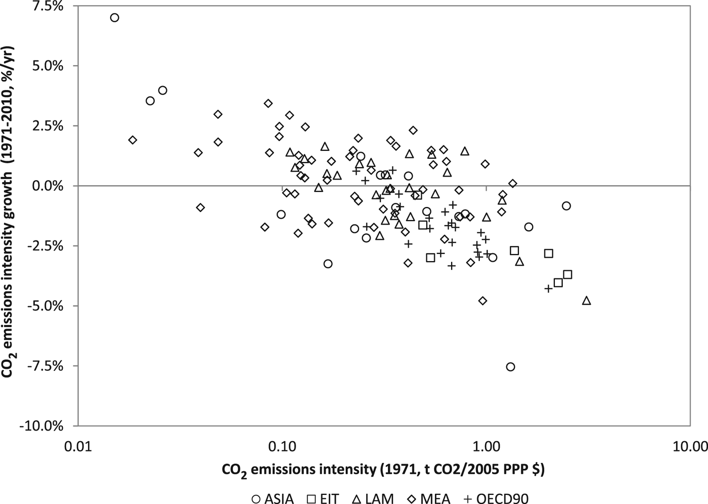
Stefanski (Reference Stefanski2013) challenges Brock and Taylor's findings, arguing that GDP growth rates have declined over time at a slower rate than emissions intensity growth rates have. Therefore, it does not make sense to argue that emissions growth has slowed mainly due to Solow-style convergence of GDP per capita growth rates. There is a strong negative relationship between countries’ initial level of emissions intensity and their subsequent emissions intensity growth rate (figure 5), which will be captured in our model.
Convergence in carbon dioxide emissions intensity

Ordás Criado et al. (Reference Ordás Criado, Valente and Stengos2011) developed a neoclassical growth model that finds that, along the optimal path, pollution growth rates are positively related to the growth rate of output and negatively related to emission levels. The origin of the latter is because utility is a function of both consumption of goods and the level of pollution, and defensive expenditures can be used to reduce pollution. Econometrically, this model reduces to a beta convergence equation with the addition of an economic growth effect. They estimate the model for a panel of 25 European countries from 1980 to 2005 using 5-year period averages. Parametric estimates for per capita SO2 emissions find that the rate of convergence is −0.021, the emissions–income elasticity is 0.653, and there are strong negative time effects, particularly in countries with initially high levels of income. For NO x the rate of convergence is −0.036 and there are again strong negative time effects, but the initial level of income has only a small and not very significant effect. Non-parametric estimates largely confirm their parametric estimates.
The Ordás Criado et al. (Reference Ordás Criado, Valente and Stengos2011) The model is a more elegant theoretical model than the green Solow model and, due to the significance of the growth and initial income terms, the model explains more of the variation in the data (in their SO2 model). As we will see in the following section, our model combines the Ordás Criado and EKC models in a single framework. However, the initial level of per capita emissions could explain the growth rate of per capita emissions for reasons besides the defensive expenditures effect, such as the diffusion of technology from low-emissions countries to high-emissions countries. Therefore, we do not interpret our results exclusively in the light of Ordás Criado et al.'s (2011) theoretical model.
3. Hypotheses, models and methods
We are agnostic about the data-generating processes for per capita GDP and emissions. It is likely, as shown by Wagner (Reference Wagner2008) and others, that both are stochastically trending (I(1)) variables, which may or may not cointegrate. Hence our adoption of the long-run growth rates representation, which should be robust for both stochastically and deterministically trending data (Chirinko et al., Reference Chirinko, Fazzari and Meyer2011). An interaction term between the economic growth rate and the initial level of income allows us to capture heterogeneity in the emissions–income elasticity. Our conceptual model is:
 $$\hat{E}_{i}=\alpha_{0}+\alpha_{1}\hat{G}_{i}+\beta^{\prime}X_{i}+\varepsilon_{i},$$
where hats indicate long-run growth rates, i.e.,
 $\hat{E}_{i}=\lpar E_{iT}-E_{i0} \rpar /T$
and
 $\hat{G}_{i}=\lpar G_{iT}-G_{i0} \rpar /T$
, where T is the final year of the time series in levels, 0 indicates the initial year, and i indexes countries.Footnote
8
E is the log of emissions per capita, and G is the log of GDP per capita. X
i
is a vector of explanatory and control variables. We deduct the sample mean from each of the continuous levels variables in this vector. α1 is an estimate of the emissions–income elasticity, which we expect to be positive, and α0 is an estimate of the mean of Ê
i
for countries with zero economic growth, the continuous levels variables at their sample means, and the dummy variables at their default value of zero. This is equivalent to the average time effect in traditional panel data EKC models. If α0<0, then in the absence of economic growth (and when the other variables are at their mean or default values), there is on average a reduction in per capita emissions over time, and vice versa.
By carefully choosing the explanatory variables, we can test hypotheses about different mechanisms that drive emissions. In particular, we propose:
 $$\hat{E}_{i}=\alpha_{0}+\alpha_{1}\hat{G}_{i}+\beta_{1}\hat{G}_{i}G_{i0}+\beta_{2}E_{i0}+\beta_{3}G_{i0}+\sum\limits_{j=4}^k {\beta_{j}X_{ji}} +\varepsilon_{i}.$$
The third term on the RHS,
 $\thinspace \hat{G}_{i}G_{i0}$
, is the interaction between the rate of economic growth and the initial level of log income per capita. This term is intended to test the EKC hypothesis that there is a level of per capita income, a ‘turning point’, so that, ceteris paribus, economic growth is associated with a decline in per capita emissions when per capita income increases above a threshold.Footnote
9
We will refer to it as the ‘EKC interaction term’.
For the EKC hypothesis to hold, β1 must be significantly less than zero. Assuming that α1>0 and β1<0, we can compute the EKC turning point where
 ${\partial \hat{E}\over \partial \hat{G}}=0$
as
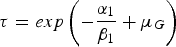 $\tau =exp\left( -{\alpha_{1}\over \beta_{1}}+\mu_{G} \right)$
, where μ
G
is the cross-country mean of initial GDP per capita that was deducted from the initial level of the GDP per capita variable prior to estimation. We use the delta method to compute the standard error of τ. If β1 is significantly less than zero but the EKC turning point is above the maximum per capita income in the sample, we can conclude that, while the emissions–income elasticity is lower for countries with higher GDP per capita, it does not fall to or below zero as would be required for an EKC downturn.
The fourth and fifth terms of (2) are the initial levels of emissions and income, included to test convergence-type theories. If β2<0, then there is beta convergence in the level of emissions per capita. If
 $\beta_{3}=-\beta_{2}$
then there is beta convergence in emissions intensity without an additional effect of the initial level of income on the emissions growth rate. The remaining X
j
are control variables, discussed below. We include these controls in each of our restricted models, although they do not appear in the original models in the literature. These control variables effectively allow the time effects to vary across countries as in Vollebergh et al. (Reference Vollebergh, Melenberg and Dijkgraaf2009).
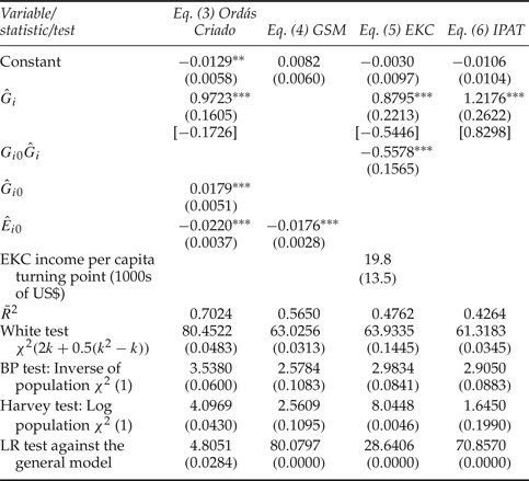
By applying restrictions to (2) we can test whether simpler specifications are adequate representations of the data. We formally test each of the exclusion restrictions, which define equations (3)–(6), using likelihood ratio (LR) tests. First, we can set β1=0, which defines the Ordás Criado et al. (Reference Ordás Criado, Valente and Stengos2011) model:
 $$\hat{E}_{i}=\alpha_{0}+\alpha_{1}\hat{G}_{i}+\beta_{2}E_{i0}+\beta_{3}G_{i0}+\sum\limits_{j=4}^k {\beta_{j}X_{ji}} +\varepsilon_{i}.$$
We would expect α1>0 and β2<0. Figure 5 shows that the correlation between the initial emissions intensity and the subsequent growth in emissions intensity is higher than that between initial emissions per capita and its subsequent growth rate illustrated in figure 4. Countries such as China that initially had high emissions intensity (and low per capita emissions) have had large decreases in emissions intensity. This suggests that it is indeed likely to be important to include the initial level of income per capita as well as the initial level of emissions per capita.
To derive the short green Solow model (Brock and Taylor, Reference Brock and Taylor2010), we set
 $\alpha_{1}=\beta_{1}=\beta_{3}=0$
:
 $$\hat{E}_{i}=\alpha_{0}+\beta_{2}E_{i0}+\sum\limits_{j=4}^k {\beta_{j}X_{ji}} +\varepsilon_{i}.$$
We would again expect β2<0. To derive a basic EKC model in growth rates without the initial per capita emissions and income terms, we set
 $\beta_{2}=\beta_{3}=0$
:
 $$\hat{E}_{i}=\alpha_{0}+\alpha_{1}\hat{G}_{i}+\beta_{1}\hat{G}_{i}G_{i0}+\sum\limits_{j=4}^k {\beta_{j}X_{ji}} +\varepsilon_{i}.$$
We would expect α1>0 and β1<0. Finally, we set
 $\beta_{1} = \beta_{2} = \beta_{3} = 0$
to define a simple IPAT-inspired growth rates model:
 $$\hat{E}_{i}=\alpha_{0}+\alpha_{1}\hat{G}_{i}+\sum\limits_{j=4}^k {\beta_{j}X_{ji}} +\varepsilon_{i}.$$
Here α1=1 for a simple IPAT model if change in ‘technology’ is independent of the GDP growth rate. If α1<1, then the rate of change in the technology term in the IPAT model is correlated with the rate of economic growth.
In the following, we discuss the additional controls. A wide variety of variables have been considered in the EKC literature. Some are genuinely exogenous or predetermined, whereas others might be seen as channels through which the development process drives emissions changes. Examples of the latter are democracy, free press, good governance and lack of corruption, which have been found to both improve economic performance and reduce environmental pressure (Pellegrini and Gerlagh, Reference Pellegrini and Gerlagh2006a, Reference Pellegrini and Gerlagh2006b). Variables such as industrial structure are also clearly driven by income growth or develop alongside GDP as part of the development process. Controlling for these could be a way to test the effect of different channels of the influence of income on emissions growth. However, we are interested in testing the overall effect of per capita income and economic growth on per capita emissions growth and so our main analysis only includes variables that are predetermined or exogenous to the development process.
The exogenous variables included in equation (2) are as follows. We include dummies for non-English legal origin, as there is evidence that legal origin is relevant for per capita emissions of SO2 (Stern, Reference Stern2012). We also include a dummy for centrally planned economies in the expectation that their reforms spurred reductions in emissions intensity. We control for the effect of climate, using country averages of temperatures over the three summer months and the three winter months, as emissions may have grown more rapidly in countries with larger cooling or heating requirements. We also include the log of the value of estimated fossil fuel endowments in 1971 (Norman, Reference Norman2009), as countries that are poor in fossil fuel endowments might exhibit faster transitions to low-emission energy sources such as nuclear power and renewables. Differences in fossil fuel endowments have been found to be an important cause of heterogeneity in emissions–income paths in prior work (Burke, Reference Burke2012, Reference Burke2013; Stern, Reference Stern2012). Finally, we include the average of the log of population density; for a given level of emissions per capita, higher population density implies higher pollution concentrations and so we would expect this variable to affect efforts to reduce SO2 emissions (ceteris paribus). Higher population density may also reduce per capita energy use and thus per capita CO2 and SO2 emissions through lower transportation costs and possibly smaller living and workspaces.
We exclusively use a linear modeling approach, where our parameter estimates attempt to capture the average effects in a possibly heterogeneous sample (Angrist and Pischke, Reference Angrist and Pischke2010). We estimate all the models using OLS with heteroskedasticity-robust standard errors. We also implement three heteroskedasticity tests. First, we use White's (Reference White1980) test of general heteroskedasticity. Secondly, because emissions per capita and income per capita are means computed over populations of various sizes, the variance of these variables should be inversely related to the size of the population, which introduces grouping-related heteroskedasticity (Maddala, Reference Maddala1977). Using the delta method, we can see that the variance of the log of these means also should be inversely related to the size of the population. We test whether this is the case, using the Breusch–Pagan test (Breusch and Pagan, Reference Breusch and Pagan1979), which involves regressing the squared residuals from each regression on the reciprocal of the mean over time of population.Footnote 10 Thirdly, it is possible that, due to measurement errors, the variance of the error term is not linearly related to the size of the population, but instead to a power of it. To test this we use the Harvey (Reference Harvey1976) test where we regress the log of the squared residuals on the log of population. We also estimate models using weighted least squares (WLS) where the error variance is assumed to be inversely proportional to population.
We assume that the explanatory variables in our regressions are exogenous. Clearly, there can be no reverse causality from growth rates to initial values. There is potentially feedback from the growth rate of emissions to the growth rate of income if either (a) local pollutants affect national economic growth, or (b) as in the case for CO2 emissions, emissions growth is tied to growth in energy use, which itself likely contributes to economic growth. Omitted variables bias may also be important as there are many variables that may be correlated with GDP or GDP growth, and which may help explain emissions growth. Finally, measurement error is a significant issue in the estimation of both GDP and emissions.Footnote 11 Usually, measurement error in GDP would be expected to bias the estimates of the regression coefficients toward zero (Hausman, Reference Hausman2001).
A common way to deal with these issues is to use instrumental variables. However, it is hard to find plausible instrumental variables (Bazzi and Clemens, Reference Bazzi and Clemens2013), especially for long-run growth rates or levels of the variables. Csereklyei and Stern (Reference Csereklyei and Stern2015) suggest that the magnitude of the bias due to reverse causality is likely to be small. The differencing we use to generate growth rates removes country-levels effects and hence one source of unexplained heterogeneity. Using long-run growth rates should reduce the effect of measurement error on the estimates (Hauk and Wacziarg, Reference Hauk and Wacziarg2009).
4. Data
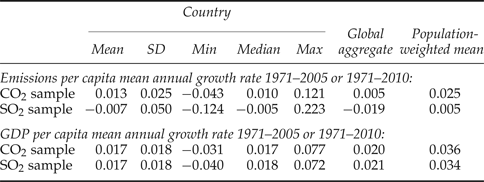
The online appendix, available at https://doi.org/10.1017/S1355770X17000109, describes the data sources in detail. Table 1 presents descriptive statistics for the growth rates of income and emissions per capita. The first five columns present statistics for the distribution of the country-level per capita income growth rates and mean (over time) per capita income levels. The sixth presents data for global-aggregate income and emissions per capita.Footnote 12 The final column provides population-weighted means of the country-level growth rates.
Descriptive statistics

Notes: Growth rates are presented in fractions rather than percentages, as that is the way the data are used in our regression analysis. The first five columns present unweighted statistics for our sample when computing the statistics for each country separately first. In the sixth column (global), we first compute the total emissions, GDP, and population for our sample of countries, and then compute the mean annual growth rate and mean per capita level of this global aggregate. In the final column we compute the growth rates using population-weighted regressions of the country-level growth rates on a constant.
Per capita CO2 emissions are rising on average across countries by more than 1 per cent per annum while per capita SO2 emissions are falling at 0.7 per cent per annum on average. Variations in the rate of change across countries are much larger for SO2 emissions than for carbon emissions, as the standard deviation of the per capita SO2 emissions growth rate is twice as large as that for per capita carbon emissions. GDP per capita has on average grown a little faster than per capita CO2 emissions, with a bit less variation across countries. There do not seem to be important differences between the distributions of the GDP per capita growth rates. Based on these simple statistics, the naïve estimates of the emissions–income elasticity would be 0.75 and −0.39 for the two data sets. As we will see, separating the total effect into time and growth effects greatly modifies the latter estimate.
The growth rates of global-aggregate per capita emissions are much lower than the unweighted country mean, while the population-weighted means are much higher. This is because, due to convergence, countries with higher initial per capita emissions saw slower growth in per capita emissions, while China and India, which have the largest populations, had rapid economic growth and rapid growth in per capita emissions.
5. Results
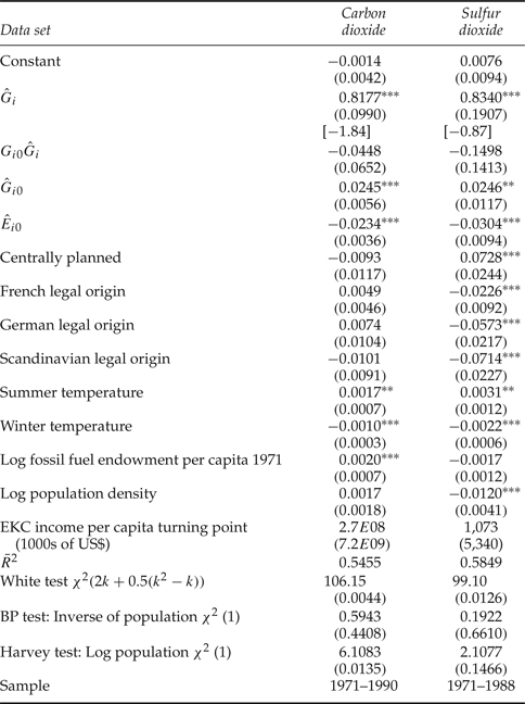
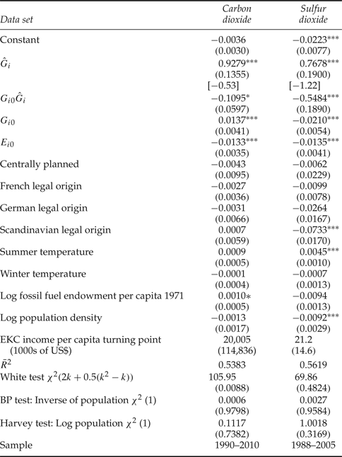
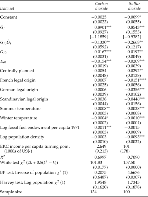
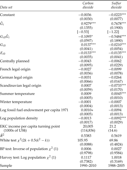
Table 2 presents the results for equation (2) for both pollutants, table 3 and 4 present the results for restricted models, and table 5–6 present results for (2) where the sample is split into two sub-periods.
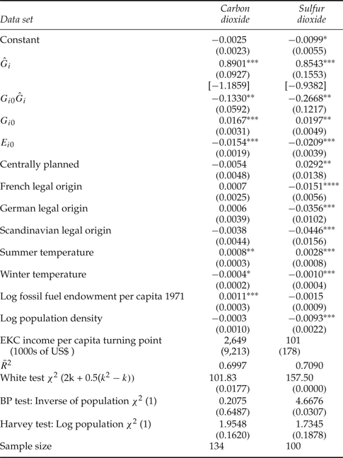
General model (equation (2))
Notes: Figures in parentheses are standard errors for the regression coefficients and the EKC turning point and p-values for White, Breusch–Pagan (BP) and Harvey test statistics. Figures in square brackets are the t-statistic for the difference between the coefficient and unity. k is the number of non-constant regressors. Significance levels of regression coefficients: *10%,
 $^{\ast\ast}{\%}$
,
 $^{\ast\ast\ast}1{\%}$
. The sample mean is subtracted from all levels variables except dummy variables so that the intercept is an estimate of the mean of Ê
i
for countries with zero economic growth, the continuous levels variables at the sample mean and the dummy variables at their default value of zero. See online appendix for further information on variable definitions.
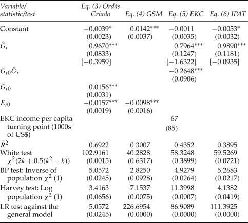
Restricted models: carbon emissions 1971–2010
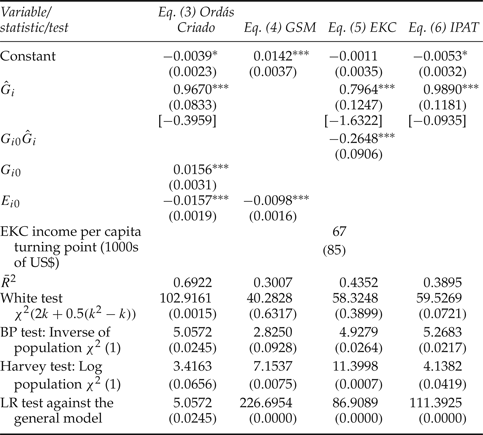
Notes: 134 data points. Control variables are also included but their coefficients are not reported. Figures in parentheses are standard errors for the regression coefficients and the EKC turning point and p-values for the White, Breusch–Pagan, Harvey and LR test statistics. Figures in square brackets are the t-statistic for the difference between the coefficient and unity. k is the number of non-constant regressors. Significance levels of regression coefficients: *10%, ***1%. The sample mean is subtracted from all continuous levels variables.
Restricted models: sulfur dioxide 1971–2005
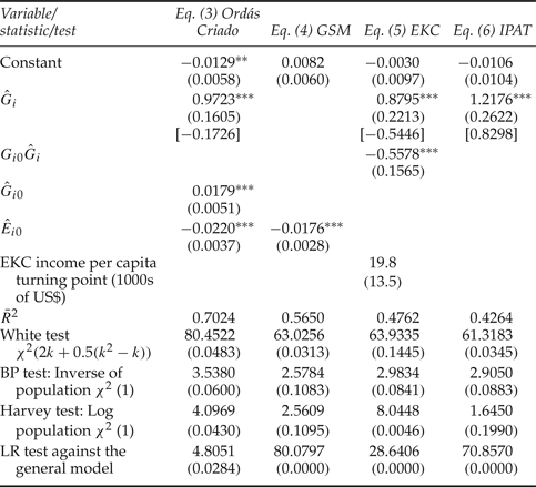
Notes: 100 data points. Control variables are also included but their coefficients are not reported. Figures in parentheses are standard errors for the regression coefficients and the EKC turning point and p-values for the White, Breusch–Pagan, Harvey and LR test statistics. Figures in square brackets are the t-statistic for the difference between the coefficient and unity. k is the number of non-constant regressors. Significance levels of regression coefficients: **5%, ***1%. The sample mean is subtracted from all continuous levels variables.
Equation (2) period 1
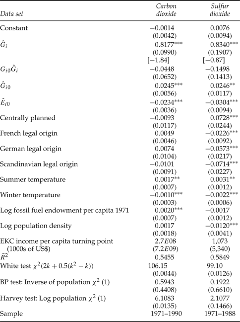
Notes: Figures in parentheses are standard errors for the regression coefficients and the EKC turning point and p-values for heteroskedasticity test statistics. Figures in square brackets are the t-statistic for the difference between the coefficient and unity. k is the number of non-constant regressors. Significance levels of regression coefficients: **5%, ***1%. The sample mean is subtracted from all continuous levels variables. See online appendix for further information on variable definitions.
Equation (2) period 2
Notes: Figures in parentheses are standard errors for the regression coefficients and the EKC turning point and p-values for heteroskedasticity test statistics. Figures in square brackets are the t-statistic for the difference between the coefficient and unity. k is the number of non-constant regressors. Significance levels of regression coefficients: *10%, ***1%. The sample mean is subtracted from all continuous levels variables. See online appendix for further information on variable definitions.
Both models in table 2 explain about 70 per cent of the variation in the data. The time effects are negative but not significant for CO2, and significantly negative (1 per cent per annum) for SO2. The emissions–income elasticity, which ranges from 0.85 to 0.93, is insignificantly different from unity for both CO2 and SO2. The coefficient of the interaction term between growth and the level of GDP per capita is negative and significantly different from zero for both. There is thus some evidence that the emissions–income elasticity is lower for countries at higher per capita income levels. This elasticity does not become negative within the observed range of GDP per capita, however, meaning that any EKC turning point is out of sample.
The coefficients of log initial GDP per capita and log initial emissions per capita are similar, but larger in absolute value for SO2. Strikingly, the annual rate of conditional convergence for per capita CO2 and SO2 is similar to the ‘iron-law’ rate of conditional convergence in GDP per capita of 2 per cent reported by Barro (Reference Barro2015). If we re-parameterize the model for initial emissions intensity rather than initial emissions per capita, then the remaining effect of initial income per capita is very small.Footnote 13 The effects of summer and winter temperature are both statistically significant and similar across the data sets with, again, a larger effect for SO2. Summer temperature has a positive effect on emissions growth, perhaps because of increasing use of air conditioning in hot countries. The coefficient is largest for per capita SO2 emissions, which are mostly produced as a result of electricity generation. Higher winter temperatures have a negative effect on per capita emissions growth, but this is smaller in absolute value than the effect of higher summer temperatures.
The coefficients of the remaining variables are very different for CO2 and SO2. Legal origin has no significant effect on per capita CO2 emissions growth, but countries with non-English legal origin saw a much more rapid decline in per capita SO2 emissions than the English legal origin countries, confirming previous findings (Stern, Reference Stern2005, Reference Stern2012). To date SO2 emissions have received more active policy attention than CO2 emissions; therefore differences in legal and regulatory regimes are more likely to have resulted in different outcomes. Formerly centrally planned status has a significantly positive effect on per capita SO2 emissions growth, ceteris paribus. As there was a rapid decline in energy intensity in these countries following liberalization, we would expect emissions to decline more rapidly in reforming economies. However, as we see in table 5, they grew much more rapidly in the centrally planned economies prior to reform and this effect dominates the full sample results.
A larger fossil fuel endowment increases the rate of growth of per capita CO2 emissions, as we would expect (Burke, Reference Burke2010, Reference Burke2012; Stern, Reference Stern2012), but does not have a significant effect on per capita SO2 emissions.Footnote 14 Population density has a strong negative effect on SO2 as expected and a smaller and insignificant effect on CO2.
Looking at the diagnostic statistics, the Breusch–Pagan test statistic for a specific theory-based heteroskedasticity structure is statistically significant at the 5 per cent level for SO2 but the Harvey test does not find that there is significant heteroskedasticity for either of these models. Population weighted WLS estimates (not reported) are, therefore, close or qualitatively similar to the OLS estimates, which means that countries with small populations that are potential outliers do not affect the results substantially. White test statistics for heteroskedasticity of an unknown form are highly significant, which justifies the use of heteroscedasticity-robust standard errors.
We also tested for the effects of some other variables that are not reported in these main results. Although energy prices are not exogenous, there is interest in their effect on the growth of emissions. In the absence of data for other fuel prices for our large international sample, we use the log of the retail price of road-sector gasoline as a proxy of country-by-country fossil fuel prices. Adding this variable to equation (2) for the CO2 data, the coefficient is −0.0099 (0.0026). The main changes in the other parameters are as follows. The coefficient on the EKC interaction term becomes insignificant. The coefficient on the fossil fuel endowment becomes much smaller and only significant at the 10 per cent level. Therefore, greater fossil fuel endowments are correlated with lower gasoline prices (Burke and Nishitateno, Reference Burke and Nishitateno2013) and the slightly lower emissions–income elasticity that was present for countries at higher initial GDP per capita levels appears to be partly related to higher fuel prices in these countries. The gasoline price has a negative but insignificant coefficient for the SO2 data set. Due to the large literature on the relationship between trade and the environment, which also inspired the first study of the EKC (Grossman and Krueger, Reference Grossman and Krueger1991), we also tested for the effect of trade openness. When added to (2) its coefficient is positive. This effect is not statistically significant at the 5 per cent level for CO2 but it is for SO2 (with a coefficient of 0.0159 (0.0047)). We also added dummies for the five regions shown in the figures. These had statistically significant effects for SO2 but generally not for CO2, and did not change the results qualitatively. We also considered the potential effects of hydroelectric power (Burke, Reference Burke2010, Reference Burke2013) by controlling for freshwater resources per capita. This variable was statistically insignificant.
Looking at tables 3 and 4, the restricted models can be rejected at the 5 per cent significance level. We thus conclude that our general specification is preferable. In both cases, the Ordás Criado et al. (Reference Ordás Criado, Valente and Stengos2011) model (3) has a much higher adjusted R-squared than the other restricted models and cannot be rejected at the 1 per cent level. Both the growth and beta convergence effects are thus important in explaining emissions. Models including convergence effects explain much more of the variation in the dependent variable than does the basic EKC model (5). The green Solow model (4) explains the least for CO2, although it is a better fit than the EKC model for SO2. The time effect for the green Solow model is positive and statistically significant for CO2, because of the elimination of the growth effect. For the EKC model, the turning points are smaller than in equation (2). For SO2 the income turning point is at US$20,000, although this estimate has a large standard error (p=0.142).
To explore whether effects varied over time, we split the sample period in half and re-estimated equation (2) for the two sub-periods 1971–1990 and 1990–2010 for CO2 and 1971–1988 and 1988–2005 for SO2 separately. Tables 5 and 6 report these results. The findings that economic growth and emissions convergence are significant drivers of emissions growth and that there is either no meaningful EKC turning point or a high EKC turning point are robust across the separate sample periods. But this sub-period analysis reveals some interesting stories. The EKC interaction term is insignificant in the first period for both pollutants and becomes more negative and highly significant for SO2 in the second period. The income turning point for SO2 also moves into the sample range (US$21,000), but remains statistically insignificant. For SO2, the time effect becomes significant and negative only in the second period. As might be expected, the coefficient for centrally planned economies is very positive and significant in the first period and becomes negative, though insignificant, in the second. Initial income has a strong negative effect for SO2 in this second period, but only Scandinavian legal origin has a significantly negative coefficient in the second period. So, after 1988 when efforts to reduce acid rain intensified (Stern, Reference Stern2005), per capita SO2 emissions began to fall everywhere in the absence of growth, particularly in high-income countries and especially in Scandinavia. The effect of winter temperatures disappears for both pollutants in the second period.
6. Discussion and conclusions
We have pursued a new long-run growth rates approach to emissions modeling that allows tests of competing explanations for emissions trajectories and nests the prior models of Ordás Criado et al. (Reference Ordás Criado, Valente and Stengos2011), Brock and Taylor, (Reference Brock and Taylor2010) and the EKC. We find that the effect of income growth on emissions is strongly positive, with a mean elasticity slightly below unity for both per capita CO2 and SO2 emissions. However, a simple per capita GDP growth rates model is not sufficient to explain changes in per capita emissions. Beta convergence effects, in particular, add considerable explanatory power for country-level emissions.
Interaction terms between income growth and the initial level of log per capita income are negative and statistically significantly for both CO2 and SO2. While this provides some evidence that the emissions–income elasticity is lower in higher income countries, any EKC per capita income turning point is well out of sample and statistically insignificant for both pollutants for the full period. We thus conclude that there is no practically important EKC in the full sample for either CO2 or SO2. For SO2, this supports conclusions first drawn by List and Gallet (Reference List and Gallet1999) and Stern and Common (Reference Stern and Common2001), although they used formulations in levels rather than growth rates. In the post-1988 period there is an in-sample turning point for SO2, but it is imprecisely estimated.
There is a strong negative time effect for SO2 ranging from −1.0 to −2.2 per cent p.a. Time effects for CO2 are not statistically significant. We find strong evidence of convergence across countries in either emissions per capita or emissions intensity. Our estimates of the green Solow model for per capita CO2 emissions have lower adjusted R-squared values than any of our models that include the growth rate of GDP. We therefore conclude that, although both are important, economic growth explains more of the variation in per capita CO2 emissions growth rates than convergence does. However, for SO2 we find the reverse: convergence has greater explanatory power than GDP growth or the EKC interaction term.
Our results provide smaller elasticities of emissions with respect to income and smaller time effects for CO2 than Stern (Reference Stern2010). This suggests that Stern's, (Reference Stern2010) results are biased by omitted variables. Perhaps this is also the case for the results of Wagner (Reference Wagner2008) and Vollebergh et al. (Reference Vollebergh, Melenberg and Dijkgraaf2009), who also use models in levels.
In summary, both growth and convergence effects are important, as proposed by Ordás Criado et al. (Reference Ordás Criado, Valente and Stengos2011). The implication is that observed cases of per capita CO2 emissions flattening in some high-income countries are not due to a natural tendency of per capita emissions to come down with time or at higher per capita income levels, but more likely are outlier countries returning to the mean, despite a robust underlying income-driven upward trend. For SO2, the data are suggestive of a more optimistic perspective, with a strong downward trend driven by technology, and per capita emissions leveling off and perhaps falling at higher per capita income levels in more recent decades. Of course, decline in per capita emissions is not a guarantee of a decline in total emissions, as the latter depends on the rate of population growth as well.
Although we find that beta convergence is important for both SO2 and CO2 per capita emissions, our analysis does not explain why. Convergence could be due to globalization leading to economic structures and the technologies used across countries becoming more similar over time, or due to countries with high emissions intensities taking policy action to improve their environments (Ordás Criado et al., Reference Ordás Criado, Valente and Stengos2011) and/or reduce their dependence on imported energy. We also found evidence on the effect of economic scarcity: countries with more abundant fossil fuel endowments have faster emissions growth. For SO2, the evidence provides more support for a policy-induced effect, visible through lower emissions in densely populated areas and strong effects of legal origin variables.
No method can address all potential issues. The fact that long-run GDP growth rates filter out non-stationary dynamics, short-run relations, time varying time-effects, and variables that might explain variation in the initial level of emissions across countries means that we cannot use our approach to assess these important issues. For example, variation in countries’ initial levels of emissions is left unexplained. This omission is shared with the panel data approach with country fixed effects. Also, we do not consider the effect of the business cycle on emissions (see Burke et al., Reference Burke, Shahiduzzaman and Stern2015). The approach we follow focuses on identifying the long-term effects of economic growth on emissions.
Supplementary material and methods
To view supplementary material for this article, please visit https://doi.org/10.1017/S1355770X17000109.