2.1 Equations of motion for turbulent channel flow

Consider the incompressible NSEs in a Cartesian coordinate system for the flow of a Newtonian fluid in the absence of external or body forces. Streamwise, wall-normal and spanwise directions will be denoted $\boldsymbol{x}=(x,y,z)$ , with corresponding (instantaneous) velocity components $\hat{\boldsymbol{U}}=({\mathcal{U}},{\mathcal{V}},{\mathcal{W}})$ and pressure ${\mathcal{P}}$ (with general spatial dependence implied but not stated explicitly for simplicity of notation). Length scales are made non-dimensional using the channel half-height, $h$ , and time scales with $u_{\unicode[STIX]{x1D70F}}/h$ , where $u_{\unicode[STIX]{x1D70F}}=\sqrt{\unicode[STIX]{x1D70F}_{w}/\unicode[STIX]{x1D70C}}$ is the friction velocity, $\unicode[STIX]{x1D70C}$ is the density and $\unicode[STIX]{x1D70F}_{w}$ is the mean wall shear stress. Then, the bulk Reynolds number, $Re_{h}=hU_{b}/\unicode[STIX]{x1D708}$ , is defined in terms of $h$ , the bulk velocity, $U_{b}$ , and the kinematic viscosity, $\unicode[STIX]{x1D708}$ , while the friction Reynolds number is $Re_{\unicode[STIX]{x1D70F}}=hu_{\unicode[STIX]{x1D70F}}/\unicode[STIX]{x1D708}$ . We denote the centreline (maximum mean) velocity by $U_{max}$ .

Employing the Reynolds decomposition, we define the (temporal) mean and fluctuating components by upper and lower case variables respectively and employ both vector and indicial notation,

The (non-dimensional) NSEs can then be written as

For mathematical simplicity, the treatment will be established for statistically stationary (steady) fully developed (one-dimensional, i.e. homogeneous in the wall-parallel directions in the mean sense) parallel flow in a channel; however, extensions to other geometries are possible for the techniques described herein, and results from pipes, and boundary layers under the quasi-parallel assumption, will also be presented.

We introduce the simplifications appropriate for wall flows that are spatially homogeneous in the $x$ and $z$ directions. Thus, the mean velocity is a function only of wall-normal distance for a given Reynolds number, and

No-slip and no-penetration boundary conditions at the walls, defined by $y=0$ and $y=2$ , and a domain that is infinitely long in the streamwise and spanwise directions are assumed.

The mean flow is governed by

As is well known, the mean equation is not closed due to the introduction of second-order statistics in an equation for a first-order term through the gradients of the Reynolds stresses, the well-known turbulence closure problem. The reader is referred to the literature on closures for the RANS equations for a direct discussion of this issue; the treatment here targets a representation of the whole flow rather than solution for only the mean velocity.

The fluctuations are governed by

2.2 Energy production, energy transfer and scale interactions

The classical energetic picture for general stationary flows in wall turbulence is of energy production at the large scales, energy transfer to smaller scales via a turbulence cascade and energy transport in physical space, with the cascade terminated via viscous dissipation at the smallest scales. The reader is referred to, e.g., Tennekes & Lumley (Reference Tennekes and Lumley1999), Pope (Reference Pope2000) and Jiménez (Reference Jiménez2012) for a more detailed description of the nonlinear scale interactions implied by this picture.

We briefly comment on the requirement for energy equilibrium, namely that total production equals total dissipation. This could equally be described as the condition for an isolated turbulent mechanism to be self-sustaining, in the sense that it could then be described as energy-neutral.

While the picture thus far is conceptually rooted in physical space and without a rigorous definition of scale, the picture of interactions between scales is mathematically simple in Fourier space. This will be exploited in the development that follows, with the caveat that the inhomogeneity in the wall-normal direction associated with the presence of a wall introduces its own complications to spectral analysis of wall turbulence.

2.3 Brief review of scaling and coherent structure in wall turbulence

Recent comprehensive treatises on the state of the art in our understanding of scaling, coherent structure and theoretical advances in wall turbulence have been given by Adrian (Reference Adrian2007), Klewicki (Reference Klewicki2010) and Smits et al. (Reference Smits, McKeon and Marusic2011), among others. Rather than duplicate works in the literature, the key concepts of relevance to this development are outlined in this section, accompanied by references for sources of more detailed information.

The differentiating feature of wall turbulence compared with most other types of turbulence is the inhomogeneity imposed by the wall. No-slip and no-penetration boundary conditions there constrain the scale and development of turbulence, and introduce a strong anisotropy into the production of turbulent kinetic energy which appears to be retained far into the cascade of energy to smaller scales. Any scaling analysis for wall turbulence will identify the importance of viscosity in meeting the wall boundary condition, an effect that is generally posited to be confined closer and closer to the wall as the Reynolds number, or the ratio of the relative importance of inertial to viscous influences, becomes higher. It should be noted that the local Reynolds number is always small near the wall.

Some of the important length scales in the flow can be identified quickly to be the viscous, or inner, length scale ( $\unicode[STIX]{x1D708}/u_{\unicode[STIX]{x1D70F}}$ ), the distance from the wall ( $yh$ ) and the outer length scale (the channel half-height, $h$ , the pipe radius, $R$ , or some measure of boundary layer thickness, $\unicode[STIX]{x1D6FF}$ ). The friction Reynolds number can be seen to be the ratio of inner to outer length scale. We define here $y^{+}=yRe_{\unicode[STIX]{x1D70F}}$ , using the superscript $+$ to denote normalization by the viscous length scale. It should be recalled that velocities have already been normalized with $u_{\unicode[STIX]{x1D70F}}$ ; use of these scales in the classical development of mean velocity scaling leads to a logarithmic dependence on distance from the wall in the so-called overlap between inner (viscous) and outer (wake) scaling.

The importance of an additional intermediate viscous (non-dimensional) length scale, namely $y_{m}=\sqrt{yy^{+}}=y^{+}/\sqrt{Re_{\unicode[STIX]{x1D70F}}}$ , has been debated for several years. See, among others, Afzal (Reference Afzal1984), Klewicki et al. (Reference Klewicki, Fife, Wei and McMurtry2007) and Klewicki (Reference Klewicki2010) for a discussion of the origin of this ‘mixed’ scaling. The scaling emerges naturally in matched asymptotic expansions (Afzal Reference Afzal1984), in the scaling of the wall-normal location of the Reynolds stress peak (Sreenivasan Reference Sreenivasan1988) and in self-similar scaling of the mean momentum balance (Klewicki et al. Reference Klewicki, Fife, Wei and McMurtry2007), and has been proposed to govern the inner limit of the log law that develops for both the mean velocity and the streamwise variance (Marusic et al. Reference Marusic, Monty, Hultmark and Smits2012) (the outer limit remains defined in outer-scaled variables).

The latter finding of a universal logarithmic region for the streamwise velocity is consistent with one of the seminal analytical results in wall turbulence, Townsend’s attached eddy hypothesis (AEH; Townsend Reference Townsend1956, Reference Townsend1961, Reference Townsend1976). As outlined in, e.g., Perry, Henbest & Chong (Reference Perry, Henbest and Chong1986), a conceptual model for coherent structures near the wall is a set of self-similar eddies that scale with distance from the wall. The tallest of these eddies contribute actively to the wall stress away from the wall, but are felt only as a large-scale ‘sloshing’, or ‘inactive motion’, by eddies closer to the wall. Analysis of the velocity field associated with such eddies leads to some seminal results, including a one-over-streamwise-wavenumber, $k_{x}^{-1}$ , scaling of the spectrum of the wall-parallel velocity fluctuations, log laws in the variances of streamwise and spanwise fluctuations as well as in the mean profile, and a region of constant variance of the wall-normal fluctuations in the same wall-normal region. Further, these outcomes appear to be relatively insensitive to the specific form of the eddies.

In terms of coherent structures, four different classes of energetic importance to wall turbulence can be identified, as catalogued by Smits et al. (Reference Smits, McKeon and Marusic2011). The near-wall cycle is commonly identified with streaks of streamwise velocity in the buffer region between the log law and the viscous sublayer, and is responsible for a peak in turbulent energy production and streamwise variance at approximately $y^{+}=15$ . Hairpin or horseshoe vortices were hypothesized (Theodorsen Reference Theodorsen1952) to dominate the near-wall and log regions, consistent with AEH ideas, and are commonly observed in experimental visualizations, at least at low and medium Reynolds numbers. Over the past two decades, the preferential relative locations of hairpin vortices, or clustering into packets, have been documented extensively. The passage of individual hairpin heads can be correlated with sweeps and ejections (contributions to net $-\overline{uv}$ arising from motion with wall-normal velocity towards and away from the wall respectively), while the clustering of ejections described as a burst seems to have its origin in the advection of a hairpin packet.

At length scales related to the outer scale, both large-scale motions (LSMs) and very-large-scale motions (VLSMs) can be identified via the streamwise spectrum in the canonical flows, (e.g. Monty et al. Reference Monty, Hutchins, Ng, Marusic and Chong2009). The LSMs, of streamwise length of the order of a couple of outer length scales, dominate the outer region, and seem to be related to bulges of turbulent activity into the more quiescent core region of internal flows, or the intermittent edge of boundary layers. The VLSMs are centred in the log region, have a footprint down to the wall and have length of order 10 times the outer length scale. The strength of the spectral signature of the VLSMs increases with increasing Reynolds number and is known to be the reason for the increasing streamwise variance near the wall and lack of inner scaling of the near-wall turbulence peak (e.g. Metzger & Klewicki Reference Metzger and Klewicki2001; Hutchins & Marusic Reference Hutchins and Marusic2007). The scale separation between the near-wall cycle and the VLSMs increases linearly with increasing Reynolds number due to the viscous scaling of the former and outer scaling of the latter.

A wide range of aspect ratios of coherent motions are observed in real turbulence; in terms of the streamwise-to-spanwise wavenumber ratio, $k_{x}/k_{z}=6{-}10$ seems to have special significance, dominating both the near-wall cycle and the VLSMs.

An important feature of the VLSMs has been elucidated over the past decade, not least in part due to the efforts of Marusic and co-workers in a series of papers identifying and characterizing the interaction of these large scales with smaller-scale turbulent activity, e.g. Mathis, Hutchins & Marusic (Reference Mathis, Hutchins and Marusic2009) and Marusic, Mathis & Hutchins (Reference Marusic, Mathis and Hutchins2010). Central to this discussion is the variation of an amplitude modulation coefficient constructed to correlate the large-scale velocity signal, $u_{L}$ , with the small-scale stress, $u_{s}^{2}$ . Here, the distinction between large and small scales is typically made using low/high-pass Fourier filters with cutoff located at wavenumber of the order of the outer scale, and the envelope, $\unicode[STIX]{x1D716}_{s}$ , of $u_{s}^{2}$ is obtained using an enveloping technique such as the Hilbert transform. Then, the amplitude modulation coefficient is defined as

where the angle brackets denote an ensemble average, typically of temporal records. Near the wall, ${\mathcal{R}}\rightarrow 1$ , and in the outer region, ${\mathcal{R}}$ takes negative values, reflecting enhanced small-scale activity near the wall within regions of high large-scale streamwise velocity and a reversing sense of activity with increasing distance from the wall. Ganapathisubramani et al. (Reference Ganapathisubramani, Hutchins, Monty, Chung and Marusic2012) have also explored related frequency modulation effects.

Jacobi & McKeon (Reference Jacobi and McKeon2013) used spectral cross-density analysis to identify that the VLSM is the major contributing scale to both $u_{L}$ and ${\mathcal{R}}$ . For a periodic signal, ${\mathcal{R}}$ can be simply interpreted as a measure of the relative phase between $u_{L}$ and $\unicode[STIX]{x1D716}_{s}$ (Chung & McKeon Reference Chung and McKeon2010), explicitly the cosine of the phase between them. A zero in ${\mathcal{R}}$ then corresponds to a $\unicode[STIX]{x03C0}/2$ difference in phase. The cosine function leaves the sense of lead or lag undetermined, but it is known from cross-correlation (Jacobi & McKeon Reference Jacobi and McKeon2013) and conditional averaging (Ganapathisubramani et al. Reference Ganapathisubramani, Hutchins, Monty, Chung and Marusic2012) that $\unicode[STIX]{x1D716}_{s}$ leads $u_{L}$ in space; given that the streamwise velocity component of the VLSM is inclined in the downstream direction, this implies that the envelope of the small scales is further inclined to the wall. Familiarity with these concepts and this phenomenology will be assumed in the following.

While turbulence is clearly a nonlinear phenomenon, recent analyses of the linear dynamics of the NSEs have given insight into the origins of fluctuations and turbulent structure. A review of key concepts is given in § 2.4. After recognizing that perturbation growth is possible in linearly stable flows (and may ultimately lead to a so-called secondary instability of the base-plus-perturbation flow), we will see that extraction of energy from the mean flow is attributable to linear mechanisms, while the nonlinearity is conservative (or passive in the controls literature) in the sense that it can only act to redistribute turbulent energy between scales, and to saturate linear amplification. The nonlinearity is important in setting the correct scales of the turbulence, but it is the linear dynamics, and specifically the coupling between wall-normal velocity and wall-normal vorticity, that control the generation and maintenance of turbulence (Kim & Lim Reference Kim and Lim2000). The role of the nonlinear terms in the NSEs, then, is essentially to ‘recycle’ the output of the linear dynamics to provide new inputs.

2.4 The picture from analysis of the linear dynamics of the NSEs

The last 20 years have seen significant research investment into the linear dynamics associated with the NSEs. In broad terms, this approach has ranged from consideration of the transient growth of disturbances that is enabled in a linearly stable flow due to the non-normality – or, strictly, lack of self-adjoint nature – of the LNSE operator (e.g. Trefethen et al. Reference Trefethen, Trefethen, Reddy and Driscoll1993), to the closed-loop representation of the NSEs as an interconnected forced linear system which will be explored in detail later.

Investigations of the linear dynamics of the turbulent NSEs originated with the quasi-laminar approach associated with a simple extension of linear instability normal mode analysis for the prediction of natural transition, as discussed in Reynolds & Hussain (Reference Reynolds and Hussain1972). Linear instability analysis of the equations of motion for turbulent flow (2.6) around the turbulent mean velocity, $U(y)$ , for small perturbations, $u_{i}$ and $p$ , is not dynamically rigorous in the sense that the turbulent mean profile is not a solution of the NSEs in the absence of the Reynolds stress gradient (but see, e.g., Sharma, Mezić & McKeon Reference Sharma, Mezić and McKeon2016a , for a formal justification). Further, the fluctuations in fully developed turbulence cannot be considered to be small. However, this approach preceded more sophisticated recent linear analyses. Reynolds & Hussain (Reference Reynolds and Hussain1972) explored improvements to the dynamical representation by including the interaction of individual fluctuation scales with the fluctuating stress field, which they term a ‘Newtonian’ eddy model with origins in the equilibrium ideas of Townsend (Reference Townsend1956). A scalar (and scale-independent) eddy viscosity, $\unicode[STIX]{x1D708}_{t}$ , is used to relate the fluctuating stress to the fluctuating strain rate, $s_{ij}$ , on a scale-by-scale basis with an individual scale denoted by $\widetilde{\cdot }$ , i.e.

and thus model the momentum transfer due to the fluctuating stresses at a given scale. In the absence of more sophisticated models, the eddy viscosity approach has been commonly used for all scales; the eddy viscosity representation proposed by Cess (Reference Cess1958) is commonly employed.

While a complete theory concerning stability of the turbulent mean profile is lacking to the best of the author’s knowledge, spectral analysis has not identified any unstable eigenmodes either with or without use of the eddy viscosity, and the profile is customarily assumed to be linearly stable. Even without unstable eigenvectors associated with the turbulent mean velocity profile, a mechanism for extraction of energy from the mean and disturbance growth exists because the linearized Navier–Stokes operator is non-normal, i.e. not self-adjoint (Trefethen & Embree Reference Trefethen and Embree2005). Further, the mechanisms of energy growth are of a three-dimensional nature, and have distinct analogy to the lift-up and Orr tilting mechanisms familiar from linear stability work, as reviewed by, e.g., Brandt (Reference Brandt2014) and Jiménez (Reference Jiménez2015). The lift-up mechanism, identified by Ellingsen & Palm (Reference Ellingsen and Palm1975) for finite amplitude streamwise-independent disturbances consisting of three velocity components, describes energy extraction from the mean due the action of a vertical fluctuation in the presence of mean shear, while Orr tilting relates to the transient energy growth associated with the tilting of initially upstream-leaning perturbations into downstream-leaning configurations by the mean shear.

As outlined by Schmid (Reference Schmid2007), analysis of the modified LNSEs can be classified relative to consideration of the homogeneous and particular solutions, representing the transient influence of initial conditions and the sustained response to external forcing respectively. For the initial condition problem, or the homogeneous solution identified above, the lack of orthogonality between (decaying) eigenvectors can lead to significant energy growth over a finite time horizon (as opposed to the infinite time horizon associated with linear instability) before the inevitable energy decay (see, for example, figure 2 of Schmid Reference Schmid2007). This phenomenon is known as transient growth. While linear stability analysis considers perturbation on a mode-by-mode basis, transient growth explicitly involves the interaction of more than one (non-orthogonal) eigenmode, and probably several for an arbitrary initial condition. The nonlinearity is assumed to kick in to saturate the process and to redistribute the energy of the disturbances between scales once the perturbation amplitudes become sufficiently large. The interested reader is referred to Schmid (Reference Schmid2007) for further background related to laminar flow, particularly with respect to mechanisms leading to the early stages of transition, and to Waleffe (Reference Waleffe1995) for a discussion of nonlinear normality versus non-normal linearity in the context of transition; our focus here is on work related to wall turbulence.

Optimal, or ‘most dangerous’, initial disturbances can be characterized which lead to the maximum gain from input to output, either globally or over a given time scale, $t$ . These optimals are defined using a suitable metric, often under an energy norm, e.g.

where $\Vert \hat{\boldsymbol{q}}(k_{x},k_{z},t)\Vert$ is the perturbation kinetic energy for the disturbance with streamwise and spanwise wavenumbers $(k_{x},k_{z})$ at a given time $t$ .

Significant amplification occurs for perturbations with $k_{x}<k_{z}$ , i.e. disturbances that are longer than they are wide, with maximum amplification obtained for very long perturbations, $k_{x}\rightarrow 0$ (Butler & Farrell Reference Butler and Farrell1993), a common result for linearized analyses. The addition of the eddy viscosity to the molecular one in the LNSE formulation appears to lead to two local maxima in $G$ for fixed (long) streamwise wavelength, associated with spanwise wavelengths of approximately $\unicode[STIX]{x1D706}_{z}=3$ and $\unicode[STIX]{x1D706}_{z}^{+}=100$ , the former experiencing the larger amplification. The optimal perturbations for both spanwise length scales consist of streamwise vortices and streaks of streamwise velocity with spacings consistent with near-wall streaks and the large structures termed ‘global structures’ by del Álamo & Jiménez (Reference del Álamo and Jiménez2006) (which seem to share characteristics with the LSMs described in § 2.3), suggesting that the linearized analysis is indeed capable of identifying structures of dynamical significance in full turbulence. This analysis has been extended to different flow configurations, including other canonical flows of relevance to this review, namely zero pressure gradient turbulent boundary layers under the quasi-parallel assumption (Cossu, Pujals & Depardon Reference Cossu, Pujals and Depardon2009) and Couette flow (Hwang & Cossu Reference Hwang and Cossu2010a ), with equivalent success.

Transient growth refers to a perturbation that ultimately decays, but sustained response can arise from the particular solution of the forced LNSEs, for which we will consider two possible input models: stochastic and harmonic forcing.

Stochastic forcing can be used as a model for intrinsic forcing with origin either internal or external to the flow. The intrinsic, or background, forcing can be posited to arise from unmodelled effects such as wall roughness, body forces, free-stream turbulence in boundary layer flows, or – of most relevance to the present development – the neglected nonlinearity in the perturbation. We will develop the conceptual picture associated with treating the nonlinearity as an unstructured forcing which is responsible for driving the linear dynamics later on, but for now note the original findings of Farrell & Ioannou (Reference Farrell and Ioannou1993), who demonstrated that small-amplitude $\unicode[STIX]{x1D6FF}$ -correlated Gaussian white-noise forcing with zero mean is capable of sustaining large perturbation variance in laminar flow. The underlying mechanism is an extraction of energy from the mean such that the variance increasingly exceeds that due to the accumulation of forcing energy as the Reynolds number is increased. The spectral distribution of energy associated with stochastic forcing can be shown to display a distinct similarity to full turbulence (Farrell & Ioannou Reference Farrell and Ioannou1998). When eddy viscosity is included in the analysis, the spanwise scale selection observed in the initial condition formulation (del Álamo & Jiménez Reference del Álamo and Jiménez2006) is also found under stochastic forcing (Hwang & Cossu Reference Hwang and Cossu2010b ). As identified by Farrell & Ioannou (Reference Farrell and Ioannou1993), the response to stochastic forcing has direct importance to modelling in that the characteristics of the input determine the space of amplified disturbances that must be spanned in order to capture the dynamics of turbulence.

Spatially distributed and temporally varying harmonic excitation can also be employed as a continuous input to the LNSEs, as either the intrinsic forcing from the neglected nonlinear terms or as an external body force field added to the right-hand side of the LNSEs. Jovanović & Bamieh (Reference Jovanović and Bamieh2005) introduced an input–output formulation of the LNSEs to assess the spatio-temporal response of channel flow to the latter case, considering external forcing with wall-normal variation, $\boldsymbol{d}(x,y,z,t)$ . Once again, the picture is of a continuous input maintaining a higher variance on output as a result of the extraction of energy from the mean flow, but with the LNSEs expressed directly in terms of a transfer function between input forcing and output (velocity/vorticity) response. Although originally formulated for laminar flow by Jovanović & Bamieh (Reference Jovanović and Bamieh2005), the concepts have been extended to a turbulent mean profile by Hwang & Cossu (Reference Hwang and Cossu2010b ) and are of particular relevance to the following.

The transfer function formulation of the LNSEs with external forcing $\boldsymbol{d}$ on the right-hand side can be written simply after taking the Fourier transform in the wall-parallel directions and in time. Denoting the Fourier transforms of $\boldsymbol{u}$ and $\boldsymbol{d}$ by $\hat{\boldsymbol{u}}$ and $\hat{\boldsymbol{d}}$ respectively, the streamwise and spanwise wavenumbers by $k_{x}$ and $k_{z}$ and the temporal frequency by $\unicode[STIX]{x1D714}$ , and introducing the spatio-temporal frequency response operator ${\mathcal{H}}(k_{x},k_{z},\unicode[STIX]{x1D714})$ as the transfer function between them,

The maximum response for a given frequency, $R(\unicode[STIX]{x1D714};k_{x},k_{z})$ , can be defined in terms of the 2-norm of the transfer function, $\Vert {\mathcal{H}}\Vert _{2}(k_{x},k_{z})$ ,

where

and $\cdot ^{\ast }$ denotes a complex conjugate.

The global maximum output response across all frequencies corresponds to the ${\mathcal{H}}_{\infty }$ norm,

where $\unicode[STIX]{x1D70E}_{max}$ is the maximum singular value associated with $\Vert {\mathcal{H}}(k_{x},k_{z},\unicode[STIX]{x1D714})\Vert$ .

The transfer function of (2.10), named the resolvent operator for a velocity field output, $\hat{\boldsymbol{u}}$ , and input, $\hat{\boldsymbol{d}}$ , can be modified to investigate component-wise transfer functions, or the influence of forcing in each direction on each component of the velocity response (Jovanović & Bamieh Reference Jovanović and Bamieh2005). In laminar flow, forcing in the cross-stream plane leads to the largest response, concentrated in the streamwise velocity component. There, the globally largest amplification occurs for streamwise-constant modes with $k_{x}=0$ , returning once again a roll/streak structure. The work of Jovanović & Bamieh (Reference Jovanović and Bamieh2005) also reveals the Reynolds number scaling of the response (not described further here).

In turbulent flow, spanwise length scales corresponding to both near-wall and global structure spacing can be identified from this analysis, consistent with the initial condition approach. The amplification of the former is independent of the Reynolds number when scaled in inner units, and that of the latter increases in amplitude with increasing Reynolds number. Further, there is evidence for geometric self-similarity of the optimal perturbations for intermediate spanwise wavenumbers (del Álamo & Jiménez Reference del Álamo and Jiménez2006; Hwang & Cossu Reference Hwang and Cossu2010b ). Interestingly, the length scales and perturbation shapes (initial and final, or input and output) arising from the initial condition problem, harmonic and stochastic forcing are essentially similar (Hwang & Cossu Reference Hwang and Cossu2010b ), underscoring the relative robustness of the NSE system and the likely dominance of perturbations of these forms in the full nonlinearly coupled system.

The remainder of this introductory section is devoted to a summary of some exact solutions of the NSEs that do not constitute the full turbulent state. The concepts are not essential to mastering the resolvent approach that is featured in the body of this article, but will be useful for understanding possible approaches to building up self-sustaining models of turbulence using this method. The first-time reader may safely skip ahead to the start of § 3.

2.5 Self-sustaining processes in wall turbulence

Self-sustenance of turbulence clearly requires retention of the nonlinearity. Besides the fully turbulent state, several nonlinear solutions that are exact in the sense that they satisfy either the full NSEs, (2.6), or specific restricted versions of the dynamical equations have been discovered in recent years. Such solutions are commonly referred to as self-sustaining processes (SSPs) in the literature. To the extent that the linear representations identify a mechanism for energy extraction and amplification relative to an assumed mean profile, one interpretation of the inclusion of the nonlinear term is that it limits the amplitudes of the linear dynamics to equilibrium values consistent with that mean velocity profile. By its very nature, a self-sustaining solution implies time independence or other symmetry in some averaged sense; we will consider here only flows with time-independent means, thus neglecting start-up transients, etc. Further, we will classify these exact solutions in terms of the nonlinear interactions that are permitted in each case.

A formal description of a streak/vortex breakdown mechanism for self-sustaining turbulence was developed by Waleffe and co-workers (e.g. Hamilton, Kim & Waleffe Reference Hamilton, Kim and Waleffe1995; Waleffe Reference Waleffe1997). In a quasi-cyclic streamwise roll/streak system, the cross-stream rolls force streamwise streaks which are unstable to a linear wave, leading to nonlinear feedback to the rolls. This picture has been explored in a range of flows, with a view to understanding the details of the interactions, including the nature of the streak instability (e.g. Schoppa & Hussain Reference Schoppa and Hussain2002) and the connection between this SSP and full turbulence. Thus, we see that the streamwise streaks and vortices that emerge from linear analysis are central to the dynamics of self-sustaining turbulence.

Jiménez & Moin (Reference Jiménez and Moin1991) defined the seminal concept of a ‘minimal unit’ of wall turbulence, or the minimum fundamental domain dimensions required for the maintenance of turbulence. This was an important advance in computation, that the essence of the near-wall turbulence cycle could be captured in a domain of limited size which explicitly excluded interaction with larger scales centred further from the wall. By systematically reducing the size of a doubly periodic channel flow direct numerical simulation (DNS) domain, it can be determined that turbulence decays for domain dimensions smaller than approximately 100 viscous units in the spanwise direction, $L_{z}^{+}\sim 100$ , in agreement with observations of streak spacing in the near-wall region of unrestricted simulations. The arguments concerning scale separation and the footprint of large structures near the wall (§ 2.3) suggest that a streamwise length scale may be harder to define and possibly not Reynolds-number-independent. However, the minimal unit representation can account for long structures through the presence of streamwise constant, $k_{x}=0$ , contributions to the minimal unit representation. The appropriate streamwise domain length appears to be at least a few hundred viscous units ( $L_{x}^{+}\sim 300$ in Jiménez & Moin Reference Jiménez and Moin1991), corresponding to the average separation of same-signed coherent vortices in the near-wall region. While no restriction is imposed in the wall-normal direction, the limitation on wall-parallel wavenumbers implied by the restricted domain essentially limits the length scales at which possible interaction with the core could occur.

Flow in the minimal unit is a representation of an SSP: no external input is required to sustain turbulence with characteristics that are in good agreement with the statistics of full (unrestricted) turbulence up to $y^{+}\sim 40$ . While the original investigation was performed at a relatively low Reynolds number ( $Re_{h}=2000{-}5000$ ) in channel flow, the near-wall cycle is understood to be quasi-universal and Reynolds-number-independent, with the implication that Reynolds-number variation of the statistics of the fluctuations near the wall has its origin in larger eddies centred further from the wall which are excluded by the $x$ and $z$ restrictions on the minimal domain.

Minimal boxes also exist further from the wall, in the logarithmic and outer scaling regions of the mean velocity. There, a streamwise streak and a vortex cluster are the dynamically important structures (Flores & Jiménez Reference Flores and Jiménez2010), and the box is wide enough to accommodate a single ejection ( $v>0$ ) and associated sweep ( $v<0$ ). In this regime, ‘minimal’ means that the box contains healthy turbulence that is self-sustaining and has the characteristics relevant to full turbulence, specifically an appropriate wall-normal extent. For healthy turbulence in these minimal boxes, the wall-normal extent scales with the box width, i.e. $y\sim L_{z}$ , and the boxes are self-similar with increasing $y$ . Smaller boxes lead to wall-normal footprints that are narrower than in real turbulence, but turbulent structures and general behaviour that are recognizably turbulent; this is in contrast to the near-wall region, where the turbulence decays if the domain is made too small. Larger boxes lead to sustained turbulence, but containing more complex turbulent structures than the minimal streak/vortex cluster unit. When the small scales are also filtered, as explored by Hwang (Reference Hwang2015) using over-damped LES to filter motions smaller than the filter length scale, the minimal box turbulence persists, and the structures can be seen to be consistent with the AEH, a useful link between one of the original scaling arguments in wall turbulence and SSPs.

2.6 Invariant solutions: restriction of the dynamics by symmetries

Great strides in developing a dynamical systems approach to the sustenance of fluctuations in the NSEs have been made over the past 25 years, as developed in Holmes, Lumley & Berkooz (Reference Holmes, Lumley and Berkooz1996). The interpretation of the nominally infinite-dimensional NSEs as a finite-dimensional dynamical system leads to a description of the coherent structure observed in transition and turbulence as the approach towards low-dimensional nonlinear invariant solutions of the NSEs. Here, ‘coherent’ denotes something – an event or phenomenon – that persists for a significant extent in both space and time. The invariant solutions can range from relatively complex strange attractors (Holmes et al. Reference Holmes, Lumley and Berkooz1996), which – at present, at least – must be extracted from data rather than by direct calculation, to the simpler forms in symmetry-restricted domains, which have been ably reviewed, for example, by Eckhardt et al. (Reference Eckhardt, Faisst, Schmiegel and Scheider2008) with regard to transition in linearly stable shear flows and Kawahara et al. (Reference Kawahara, Uhlmann and van Veen2012) for turbulent flows.

The full dynamical systems treatment has been well characterized in the review by Kawahara et al. (Reference Kawahara, Uhlmann and van Veen2012), and the details of the approach are not repeated here. However, it will be useful to review one of the types of simple solution that have been documented to date, namely the relative equilibrium states, which correspond to exact solutions in the frame of reference moving with a constant convective velocity. These are alternately called travelling wave solutions (TWSs; Gibson, Halcrow & Cvitanović Reference Gibson, Halcrow and Cvitanović2008), exact coherent states (ECSs; Waleffe Reference Waleffe2001) or, in the asymptotically high-Reynolds-number limit, vortex–wave interaction (VWI; Hall & Sherwin Reference Hall and Sherwin2010).

The first ECS solution is attributed to Nagata (Reference Nagata1990), who identified through a numerical study a non-laminar equilibrium in spatially periodic Couette flow. Waleffe (Reference Waleffe2001) subsequently formalized the description of the dynamics of the underlying SSP. Exact coherent states have been found in all of the canonical flows, in chronological order of discovery: plane Couette, channel, pipe and boundary layer flows. The reader is referred to Kawahara et al. (Reference Kawahara, Uhlmann and van Veen2012) for a review including further details of specific invariant solutions.

Exact coherent state families typically consist of so-called lower- and upper-branch solutions (also characterized in terms of streak- and vortex-dominated solutions by Kawahara et al. Reference Kawahara, Uhlmann and van Veen2012), which appear to most closely resemble laminar and turbulent flow respectively. Common features of the solutions are wavy low-speed streaks flanked by staggered quasi-streamwise vortices, a picture consistent with observations in full turbulence by, e.g., Schoppa & Hussain (Reference Schoppa and Hussain2002). At infinite Reynolds number, the mechanism for energy production is described by VWI (Hall & Smith Reference Hall and Smith1991; Hall & Sherwin Reference Hall and Sherwin2010) centred on the critical layer, the spatially varying location where the wave convection velocity, $c$ , is equal to the base velocity. The critical layer also plays an important but not completely characterized role in the dynamics of ECSs (Kawahara et al. Reference Kawahara, Uhlmann and van Veen2012; Park & Graham Reference Park and Graham2015).

While not turbulent in the formal sense, invariant solutions can be considered as tractable representations of SSPs in ‘baby turbulence’ possessing considerably less complex dynamics than the fully developed state, a feature that will be exploited later in this article. The relationships between invariant solutions and full turbulence have been explored by, e.g., Waleffe (Reference Waleffe2003) and Jiménez et al. (Reference Jiménez, Kawahara, Simens, Nagata and Shiba2005), and reviewed by Kawahara et al. (Reference Kawahara, Uhlmann and van Veen2012). Park & Graham (Reference Park and Graham2015) outline the connection between ECSs and fully turbulent simulations, observing that trajectories of a fully turbulent DNS, when expressed in the state space defined by instantaneous measures of turbulent kinetic energy (TKE), dissipation and wall shear stress, come close to several known ECS solutions.

2.7 Restricted nonlinear interactions

An alternative approach to identifying self-sustaining or exact solutions is to restrict the specific nonlinear interactions permitted. Quasi-linear models can be formulated, in which one (or more) scales beyond the mean are resolved and the remaining ‘unresolved’ scales are modelled. Formulations that admit streamwise-constant perturbations, $(k_{x},k_{z})=(0,k_{z})$ , as the resolved spatial scales have met considerable success in wall turbulence. This area has a long history (see, e.g., Farrell & Ioannou (Reference Farrell and Ioannou2014) for a detailed description), with some recent breakthroughs with regard to wall turbulence.

The streamwise-constant components of the velocity and pressure can be isolated by streamwise averaging on the domain, denoted here by $\langle \cdot \rangle _{x}$ . A streamwise-constant velocity vector, $\check{\boldsymbol{U}}(y,z,t)$ , can then be defined; this is termed the ‘mean’ flow by Farrell and co-authors, but explicitly includes fluctuations with variation in both $y$ and $z$ directions as well as the spatio-temporal mean (which is a function of $y$ only). New perturbations $\check{\boldsymbol{u}}$ relative to the streamwise-constant flow can also be defined,

and similarly for the pressure.

The governing equations for the resolved streamwise-constant flow and unresolved scales of motion have variously been called the two-dimensional three-component (2D/3C) model (e.g. Gayme et al. Reference Gayme, McKeon, Papachristodolou, Bamieh and Doyle2010), the restricted nonlinear (RNL) system (e.g. Thomas et al. Reference Thomas, Farrell, Ioannou and Gayme2015), the quasi-linear model (e.g. Marston, Chini & Tobias Reference Marston, Chini and Tobias2016) and a statistical state steady dynamics model, one example of which is the so-called stochastic structural stability theory (S3T) (e.g. Farrell & Ioannou Reference Farrell and Ioannou2014). The S3T is a ‘deterministic, autonomous, nonlinear dynamical system for evolving a second-order approximation to the statistical mean turbulent state’ (Farrell & Ioannou Reference Farrell and Ioannou2014). The RNL system represents a realizable implementation of S3T and restricts interactions that are nonlinear in the perturbations, $\check{\boldsymbol{u}}$ , to the specific interactions that lead to zero streamwise wavenumber; the streamwise-constant activity is driven using the full coupled perturbation field parameterized by a stochastic forcing. See, for example, figure 1 of Farrell et al. (Reference Farrell, Ioannou, Jiménez, Constantinou, Lozano-Duran and Nikolaidis2016) for a description of the permitted nonlinear interactions in wavenumber space in such models.

Interestingly, turbulence initialized by an external forcing can sustain itself in the presence of a limited number of streamwise-varying modes (Thomas et al. Reference Thomas, Farrell, Ioannou and Gayme2015) or when exogenous forcing is removed (Farrell et al. Reference Farrell, Ioannou, Jiménez, Constantinou, Lozano-Duran and Nikolaidis2016). The flow physics underlying such self-sustenance can be described in terms of a cooperative instability of a roll/streak structure with superimposed incoherent ‘turbulence’, in which the lift-up associated with the rolls organizes the Reynolds stress in such a way as to maintain the flow. Recently, it has been shown that roll/streak structures in RNL simulations (Farrell & Ioannou Reference Farrell and Ioannou2012) and DNS have dynamics that are formally similar (Farrell et al. Reference Farrell, Ioannou, Jiménez, Constantinou, Lozano-Duran and Nikolaidis2016), suggesting that the SSP identified from this quasi-linear approach has the potential to inform models of the mechanisms of full turbulence.

3.1 Formulation for turbulent channel flows

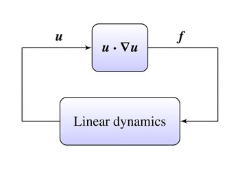
At the heart of the approach is the formulation of the NSEs in terms of a linear operator driven by nonlinear forcing (much as in the input–output analysis described in § 2.4 above, but with endogenous forcing and a closed feedback loop), as shown in the schematic in figure 1. This forcing, $\boldsymbol{f}$ , is understood to recycle the velocity output, $\boldsymbol{u}$ , into an input to the system. In what follows, the velocity and forcing will be decomposed on a scale-by-scale basis, such that a formal transfer function between them can be defined. The essence of the development then addresses three main questions: how the characteristics of this transfer function dictate which inputs experience amplification, how the equations of motion restrict the nonlinear interactions that give rise to such inputs and whether the flow is able to generate such inputs.

Figure 1.

A high-level description of the turbulence process. The lower block contains the linear dynamics of the fluctuations interacting with the mean velocity profile. After McKeon et al. (Reference McKeon, Sharma and Jacobi2013).

To progress, we consider the question of the appropriate bases for decomposition in all three spatial dimensions and in time. The analysis will be performed for a channel domain that is infinitely long in the streamwise and spanwise directions, and a flow with statistics that are homogeneous in $(x,z)$ and stationary in time as in § 2.1, such that the usual assumption of ergodicity is justified. The no-slip no-penetration wall boundary conditions are employed for the development, but we will see that variations are possible. It should be noted that the development will be given in primitive variables rather than a wall-normal velocity/vorticity formulation in order to make a straightforward comparison with experimental observations in the following sections.

The invariance of the NSEs under translation in time and in the wall-parallel directions, $x$ and $z$ , suggests that Fourier bases are not just convenient but formally appropriate in these dimensions (Sharma et al. Reference Sharma, Mezić and McKeon2016a ). Then,

with the appropriate inverse transform. Here, $\widetilde{\boldsymbol{u}}_{\boldsymbol{k}}=\widetilde{\boldsymbol{u}}_{\boldsymbol{k}}(y;k_{x},k_{z},\unicode[STIX]{x1D714})$ and $\widetilde{p}_{\boldsymbol{k}}=\widetilde{p}_{\boldsymbol{k}}(y;k_{x},k_{z},\unicode[STIX]{x1D714})$ , where $k_{x}$ and $k_{z}$ denote the streamwise and spanwise wavenumbers respectively, we will denote the wavenumber–frequency triplet by $\boldsymbol{k}=(k_{x},k_{z},\unicode[STIX]{x1D714})$ and we introduce the shorthand $\boldsymbol{k}\boldsymbol{\cdot }\boldsymbol{x}=k_{x}x+k_{z}z-\unicode[STIX]{x1D714}t$ (note the transformation of the sign of $\unicode[STIX]{x1D714}$ in the Fourier transform of (3.2) to obtain a default downstream streamwise advection for the oblique travelling wave representation for $k_{x},\unicode[STIX]{x1D714}>0$ ). The original analysis of McKeon & Sharma (Reference McKeon and Sharma2010) was formulated to consider complex frequency via a Laplace transform (and we will observe a demonstration of this configuration in § 9). At this stage of the development, we consider exclusively real $\boldsymbol{k}$ , giving rise to disturbances that are neutrally stable, i.e. with no spatial or temporal growth. The interpretation, then, is of a summation of obliquely propagating waves with a streamwise (convective) wavespeed defined by $c=\unicode[STIX]{x1D714}/k_{x}$ . It should be noted that oblique wave representations for wall turbulence have also been utilized by Landahl (Reference Landahl1967) and Sirovich, Ball & Keefe (Reference Sirovich, Ball and Keefe1990) with slightly different objectives in mind. The triple-Fourier-decomposed representation is consistent with the statistical representation of turbulence in the (customarily one- or two-dimensional) spectral domain, which will assist with direct comparisons with observations.

The general equations for the fluctuations (cf. 2.6) can be written in operator form as

with subscript $t$ denoting the derivative with respect to time. Here, we employ a compact notation, where the gradient operator $\unicode[STIX]{x1D735}=[\text{i}k_{x},\unicode[STIX]{x2202}_{y},\text{i}k_{z}]$ , the Laplacian $\unicode[STIX]{x1D6FB}^{2}=\unicode[STIX]{x2202}_{yy}-\unicode[STIX]{x1D705}^{2}$ , and $\unicode[STIX]{x2202}_{y}$ and $\unicode[STIX]{x2202}_{yy}$ denote the first and second derivatives with respect to $y$ . We define the modulus of the wavenumber vector as $\unicode[STIX]{x1D705}^{2}=k_{x}^{2}+k_{z}^{2}$ . The right-hand side of (3.4) is then the term nonlinear in the fluctuation, which we will identify directly as a forcing, $\boldsymbol{f}=-(\boldsymbol{u}\boldsymbol{\cdot }\unicode[STIX]{x1D735})\boldsymbol{u}+\overline{(\boldsymbol{u}\boldsymbol{\cdot }\unicode[STIX]{x1D735})\boldsymbol{u}}$ . Nonlinear effects have been effectively isolated in the forcing, $\boldsymbol{f}$ , and in the sustained deviation of the turbulent mean velocity, $U(y)$ , from a laminar base flow.

Fourier transforming (3.4) and (3.5), we obtain

This is essentially the LNSE representation of linear stability analysis, but with the forcing $\boldsymbol{f}_{\boldsymbol{k}}$ explicitly retained and not limited to be small. In fact, $\boldsymbol{f}_{\boldsymbol{k}}$ is constituted of the spatial gradients of the Reynolds stress at scale $\boldsymbol{k}$ ; it incorporates the convolution of all scale interactions (with the exception of the $\boldsymbol{k}=(0,0,0)$ modes, which contribute through the linear terms) that result in the given $\boldsymbol{k}$ ,

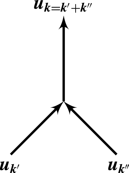
Explicitly, the integral covers the interaction of all pairs of scales $(\boldsymbol{k}^{\prime },\boldsymbol{k}^{\prime \prime })$ where $k_{x}^{\prime }+k_{x}^{\prime \prime }=k_{x}$ , $k_{z}^{\prime }+k_{z}^{\prime \prime }=k_{z}$ and $\unicode[STIX]{x1D714}^{\prime }+\unicode[STIX]{x1D714}^{\prime \prime }=\unicode[STIX]{x1D714}$ : the quadratic nature of the NSE nonlinearity leads to the well-known triadic compatibility constraint for scale interaction. The form of the nonlinear terms was given explicitly for pipe and channel flow in Sharma & McKeon (Reference Sharma and McKeon2013a ); for Cartesian coordinates and a given set of scales, $(\boldsymbol{k},\boldsymbol{k}^{\prime },\boldsymbol{k}^{\prime \prime })$ , the integrand of (3.8) can be expanded to show explicitly its relationship to the Reynolds stresses,

Now, identifying the case $\boldsymbol{k}=(0,0,0)$ as the mean flow, i.e. $\boldsymbol{u}_{0}=\boldsymbol{U}=(U,0,0)$ and $p_{0}=P$ , then

where $\boldsymbol{f}_{0}$ arises from all interactions of $\boldsymbol{k}$ with its conjugate, i.e. $\boldsymbol{k}^{\prime \prime }=-\boldsymbol{k}^{\prime }$ and

such that (2.5) is recovered, as expected.

The Reynolds decomposition performed in (2.1) and carried into this development can now be seen to be a natural step in the Fourier decomposition rather than a required linearization. Indeed, we draw a philosophical distinction between the present approach and analysis of the linearized dynamics of the NSEs. A full dynamical characterization of the connections between analysis of fluctuations about a profile that is not a solution of the NSEs and linearization remains to be fully understood, at least by this author. It should be noted also that the formulation of (3.6)–(3.7) and (3.10)–(3.11) explicitly accounts for the correct subset of all scale interactions contributing to the forcing $\boldsymbol{f}_{\boldsymbol{k}}$ without requiring the introduction of an eddy viscosity.

The equations for the fluctuations, (3.6)–(3.7), can be rearranged into a forcing–response relationship for the fluctuations, given by

where ${\mathcal{L}}_{\boldsymbol{k}}$ is the (spatial) linear Navier–Stokes operator given by

The pressure fluctuations are then recovered via the Poisson equation for pressure,

McKeon & Sharma (Reference McKeon and Sharma2010) considered a divergence-free set of basis functions that meet the wall boundary conditions (Meseguer & Trefethen Reference Meseguer and Trefethen2003) and thus precluded the necessity for direct treatment of the continuity equation. In this case, a complete transfer function relationship between velocity and intrinsic forcing (cf. (2.10) for external forcing) can be written as

Writing $\boldsymbol{f}_{\boldsymbol{k}}$ in terms of a nonlinear function of the velocity fluctuations,

$\boldsymbol{u}_{\boldsymbol{k}}$ satisfies

with the further consistency condition that the mean velocity profile incorporated in ${\mathcal{H}}_{\boldsymbol{k}}$ is correct, i.e. (3.10) holds. Equations (3.10) and (3.18) determine the velocity field, which constitutes a full solution of the NSEs.

The transfer function

can be identified as the resolvent operator. A commonly used formalism in operator theory to describe the spectral properties of an operator, the name ‘resolvent’ seems to be attributed to David Hilbert (note that the so-called ‘first resolvent identity’ is also known as ‘Hilbert’s identity’). Its history in fluid mechanics is traceable to analysis of stability and transition in shear flows (Trefethen et al. Reference Trefethen, Trefethen, Reddy and Driscoll1993; Schmid & Henningson Reference Schmid and Henningson2001; Jovanović & Bamieh Reference Jovanović and Bamieh2005), while a similar concept appears to have been first introduced for turbulent flows in the context of stochastic forcing of the LNSEs by Farrell & Ioannou (Reference Farrell and Ioannou1993). If the mean velocity profile is known, then ${\mathcal{H}}_{\boldsymbol{k}}$ can be computed for any $\boldsymbol{k}$ . It should be noted that the forcing $\boldsymbol{f}_{\boldsymbol{k}}$ can excite a response only in $\boldsymbol{u}_{\boldsymbol{k}}$ .

This analysis can be extended using the primitive variable formulation implied by (3.13) to obtain a modified resolvent formulation (Luhar, Sharma & McKeon Reference Luhar, Sharma and McKeon2014a ),

which precludes the necessity for projection of the NSEs onto a predetermined divergence-free basis. Obviously, this treatment of mass continuity leads to direct information concerning the pressure fluctuations, but it also opens the formulation to investigation of non-canonical boundary conditions (for example deforming walls or linear wall-based control laws), for which a divergence-free basis is not necessarily known a priori.

The pressure fluctuations identified by the resolvent analysis of (3.20) are related to the so-called ‘fast’ pressure or the first term on the right-hand side of (3.15), which is linear in the shear and the wall-normal velocity fluctuation; it can be shown explicitly that the ‘slow’ pressure consists of the divergence of the full forcing field, as written in (3.15), such that determination of the contribution of this term to the pressure requires solution of the full nonlinear turbulence field (Luhar et al. Reference Luhar, Sharma and McKeon2014a ).

This representation of the NSEs is exact to this point, and the novelty of the approach thus far lies in the interpretation of the mean velocity profile in the Reynolds decomposition of (2.1) and in the conceptual treatment of the nonlinearity as an intrinsic forcing, whose effects are contained in $\boldsymbol{f}_{\boldsymbol{k}}$ and $U(y)$ . The triple Fourier decomposition highlights the importance of the wall-normal location, $y_{c}$ , where $(\unicode[STIX]{x1D714}-k_{x}U)=0$ , i.e. $c=\unicode[STIX]{x1D714}/k_{x}=U(y_{c})$ and the wavespeed is equal to the local mean velocity. This location is known as the critical layer in linear stability literature; in the absence of diffusion, the resolvent is singular there (the diagonal terms in (3.19) go to zero), such that the critical layer is one potential source of high amplification of input disturbances in this formulation. The other source is the well-known coupling between the wall-normal velocity, $v$ , and the wall-normal gradient of the mean velocity, the lift-up effect described earlier.

3.2 Gain-based decomposition of the resolvent in the wall-normal direction

The basis for decomposition of the resolvent in the wall-normal direction has not yet been specified. The presence of the wall and associated inhomogeneity in $y$ mean that practical choices such as a Fourier basis or Chebyshev polynomials are not the efficient ones in terms of representing the resolvent. Thus, McKeon & Sharma (Reference McKeon and Sharma2010) selected a gain-based approach. A Schmidt decomposition for integral operators has a finite matrix equivalent in the singular value decomposition (SVD), which we use for the discretized NSEs henceforth. It should be noted that an SVD in the homogeneous directions returns Fourier modes. The essence of this technique, namely a principal component analysis, is familiar from data decomposition techniques such as proper orthogonal decomposition (POD); the approach taken here is to analyse the equations of motion, through the resolvent, rather than to analyse data.

For simplicity of explanation, we treat the resolvent formulation of (3.16) here, but note that analysis of the modified resolvent in (3.20) and the means of recovering the pressure are described in full in Luhar et al. (Reference Luhar, Sharma and McKeon2014a ).

If there are no eigenvalues of ${\mathcal{L}}_{\boldsymbol{k}}$ with zero real part, the SVD of the resolvent can be written in terms of left and right singular functions and singular values as

The singular forcing and singular velocity response (resolvent) modes, $\unicode[STIX]{x1D713}_{\boldsymbol{k},j}$ and $\unicode[STIX]{x1D719}_{\boldsymbol{k},j}$ respectively, are orthonormal, i.e.

and unique up to a complex (unitary) amplitude which corresponds to a spatio-temporal phase shift on both bases. In practice, the phases can be set with respect to a wall-normal location, such as the wall or critical layer height for a given $\boldsymbol{k}$ , for consistent interpretation of the modes. The singular values, $\unicode[STIX]{x1D70E}_{\boldsymbol{k},j}$ , are ranked,

Thus, an input $\unicode[STIX]{x1D719}_{\boldsymbol{k},j}(y)$ gives an output $\unicode[STIX]{x1D70E}_{\boldsymbol{k},j}\unicode[STIX]{x1D713}_{\boldsymbol{k},j}$ , or

and the largest amplitude output given unit forcing energy is $\unicode[STIX]{x1D70E}_{\boldsymbol{k},1}\unicode[STIX]{x1D713}_{\boldsymbol{k},1}$ in response to input $\unicode[STIX]{x1D719}_{\boldsymbol{k},1}$ . The SVD provides the optimal harmonic perturbation locally in $\boldsymbol{k}$ space rather than the more commonly sought global optimal.

More generally, any general forcing $\boldsymbol{f}_{\boldsymbol{k}}$ or velocity field $\boldsymbol{u}_{\boldsymbol{k}}$ can then be decomposed in terms of the singular functions as follows:

and

where the $\overline{\unicode[STIX]{x1D712}}_{\boldsymbol{k},j}$ are the coefficients of projection of the actual forcing onto the forcing modes. In a self-sustaining turbulent system, the forcing weights, $\overline{\unicode[STIX]{x1D712}}_{\boldsymbol{k},j}$ , are constrained to values that recycle the output velocities $\boldsymbol{u}_{\boldsymbol{k}}$ to self-consistent input forcing throughout the system. This treatment of the nonlinearity via an interconnection of otherwise linear operators is shown in figure 2, together with a summary of the key steps in the analysis.

Figure 2.

Schematic of the system representation of the resolvent formulation, after Moarref et al. (Reference Moarref, Jovanović, Sharma, Tropp and McKeon2014), reproduced with permission. Here, FT and IFT denote the Fourier transform and its inverse respectively. The blue text and arrows identify the key conceptual steps in obtaining a self-sustaining representation of turbulence.

To wrap up the mathematical foundations of this analysis, it should be noted that an interpretation in terms of the $\unicode[STIX]{x1D716}$ -pseudospectrum (Trefethen & Embree Reference Trefethen and Embree2005) of the resolvent is given in McKeon & Sharma (Reference McKeon and Sharma2010), and that the ${\mathcal{L}}_{2}$ norm of the resolvent can be shown to equal to the first singular value. We note that the SVD is formally equivalent to eigenvalue decomposition for positive semi-definite operators, a condition that is violated because of the non-normality of the resolvent. For a normal operator, an SVD would yield forcing and response functions that are complex conjugates of each other.

From consideration of (3.27), it can be seen that a large response $\boldsymbol{u}_{\boldsymbol{k}}$ to a general forcing $\boldsymbol{f}_{\boldsymbol{k}}$ can be obtained through either a large singular value, $\unicode[STIX]{x1D70E}_{\boldsymbol{k},j}$ , or a large forcing weight, $\overline{\unicode[STIX]{x1D712}}_{\boldsymbol{k},j}$ , a conceptual distinction that was discussed by Chernyshenko & Baig (Reference Chernyshenko and Baig2005). The former has a linear origin, a consequence of the mean profile, diffusion and the lift-up effect, while the latter is a nonlinear effect.

Resolvent analysis has strong connections with other modelling approaches not described herein, including rapid distortion theory, POD and dynamic mode decomposition (DMD), i.e. analysis of data rather than the equations of motion, and Koopman analysis of the equations governing nonlinear dynamical systems (Sharma et al. Reference Sharma, Mezić and McKeon2016a ). We emphasize that the retention of the true intrinsic forcing through $\boldsymbol{f}_{\boldsymbol{k}}$ under the present approach leads to an explicit representation of the dynamics in a formulation derived from the NSEs rather than empirically obtained from physical data. While the development has been given for turbulent channel flow, with a corresponding one-dimensional resolvent, the concepts can be extrapolated to a range of other non-canonical turbulent flows.

3.3 Practical implementation

Analysis of the resolvent typically proceeds with a pseudospectral discretization in the wall-normal direction on (Chebyshev) collocation points and formulation of the differential operators required. Appropriate resolution must be determined for the Reynolds number under consideration and the wall-normal footprint of $\boldsymbol{u}_{\boldsymbol{k}}$ and $\boldsymbol{f}_{\boldsymbol{k}}$ , such that the influence of high shear near the wall is fully captured in converged singular functions (see, for example, Meseguer & Trefethen Reference Meseguer and Trefethen2003, for a related study).

Formulation of the resolvent ${\mathcal{H}}_{\boldsymbol{k}}$ requires knowledge of the mean velocity profile. Progress can be made by assuming the mean profile for canonical flow as an input, as indicated in figure 2, for example using an eddy viscosity formulation or from experimental or numerical data, but (3.11) governs the fluctuation interactions driving the mean, such that a complete self-sustaining system can be formulated, as in figure 2.

The computational overhead associated with performing the SVD at a given $\boldsymbol{k}$ and Reynolds number in this implementation is extremely low. Resolvent analysis, including the results shown herein, can be performed on a laptop in MATLAB^©, using either the implicit svd or svds commands to generate the SVD (with the relative speed of these dictated by the size of the matrix) or a scheme that exploits the low-rank nature of the operator (described below) to approximate the first singular functions. The randomized approach of Halko, Martinsson & Tropp (Reference Halko, Martinsson and Tropp2011) utilizes random input and the preferential amplification associated with the rapid roll-off of singular values with increasing SVD rank to extract the most amplified inputs and outputs without the expense of the matrix inversion required by the SVD, and becomes faster and more accurate the more rapid the decay of the singular values with increasing singular mode number is. While analysis at a single $\boldsymbol{k}$ typically takes less than a second, the latter approach has been found to lead to a saving of approximately 50 % in total computational time associated with calculating velocity response modes over a wavenumber sweep compared with the basic SVD algorithm (Moarref et al. Reference Moarref, Sharma, Tropp and McKeon2013). Given the expansion of modern techniques for linear algebra, it likely that there exist additional specialized tools for these operations which are made relevant for wall turbulence by the present formulation.

3.4 Low-rank approximation of the resolvent

The resolvent has been found to be low rank for $\boldsymbol{k}$ values corresponding to known turbulence features. A limited number of preferential input directions are highly amplified, denoted by singular values that are large relative to the values for higher-order singular modes. This roll-off of the singular values with increasing singular mode order (particularly abrupt for long streamwise structures with low values of $k_{x}$ ) makes the resolvent a highly selective filter, and is a source of the apparent robustness of the structure associated with the velocity response modes which will be described in § 4.

Figure 3.

Comparison of the energy associated with the first response mode pair with $c=U(y^{+}=15)$ under broadband unit forcing in channel flow (taken from Moarref et al. Reference Moarref, Sharma, Tropp and McKeon2013, with permission), i.e. ${\mathcal{E}}(\boldsymbol{k})=(\unicode[STIX]{x1D70E}_{\boldsymbol{k},1}^{2}+\unicode[STIX]{x1D70E}_{\boldsymbol{k},2}^{2})/\sum _{j}\unicode[STIX]{x1D70E}_{\boldsymbol{k},j}^{2}$ (filled colour isocontours), with line isocontours of turbulent kinetic energy from the channel flow DNS of Hoyas & Jiménez (Reference Hoyas and Jiménez2006) at $y^{+}=15$ . Here, $\unicode[STIX]{x1D706}_{x}^{+}$ and $\unicode[STIX]{x1D706}_{z}^{+}$ are the streamwise and spanwise wavelengths normalized by the viscous length scale.

Formally, the operator can be well approximated by a highly reduced number of singular functions (see Schmid (Reference Schmid2007) or McKeon et al. (Reference McKeon, Sharma and Jacobi2013) for schematics of the input–output mapping associated with a low-rank transfer function), with the rank- $N$ approximation truncating the summations in (3.26) and (3.27) at $N$ functions,

Here, we introduce the velocity weighting,

Depending on the modelling objective, $N=1{-}10$ typically gives a good representation of experimentally observed structures and velocity spectra (see §§ 4 and 11 respectively).

Wall turbulence ‘lives’ where the resolvent operator is low rank. Figure 3, from Moarref et al. (Reference Moarref, Sharma, Tropp and McKeon2013), shows a comparison between the line isocontours of the spatial turbulent kinetic energy spectrum from the DNS of Hoyas & Jiménez (Reference Hoyas and Jiménez2006) at a wall-normal distance corresponding to the peak activity of the near-wall cycle, $y^{+}=15$ , with the (filled) isocontours of fractional energy, ${\mathcal{E}}(\boldsymbol{k})$ , of the response contained in the first two velocity response modes (consisting of a symmetric and anti-symmetric mode pair). Broadband forcing is assumed, i.e. unit amplitude excitation of all singular forcing modes, to the resolvent operators with the spatial wavelengths shown and frequency determined by matching the wavespeed, $c$ , with the mean velocity, i.e. $\unicode[STIX]{x1D714}=k_{x}U(y^{+}=15)$ , such that

The TKE isocontours overlap the region of the most low-rank behaviour, which is centred around the peak in near-wall activity. One can note the imprint of TKE from structures sitting higher above the wall and with higher convection velocity at large $(\unicode[STIX]{x1D706}_{x}^{+},\unicode[STIX]{x1D706}_{z}^{+})$ , and the lack of overlap at the highest streamwise wavelengths, where the amplification is known to be highest. We will return to this conundrum.

3.5 Turbulent field representation in terms of response functions

The oblique travelling wave interpretation of (3.3) together with the low-rank nature of the resolvent allows a novel representation of the flow in a discretized domain. Once the mean profile is known, the singular velocity response modes can be calculated offline, such that the entire field is determined (approximated) by the four-dimensional complex weighting coefficients, $\unicode[STIX]{x1D712}_{\boldsymbol{k},j}$ (or $\overline{\unicode[STIX]{x1D712}}_{\boldsymbol{k},j}$ ), with $j=1:N$ .

Figure 4 outlines this representation for the rank- $N$ representation of the resolvent (a), and for the rank-1 approximation that will be used as far as possible in the following (b,c). The minimum and maximum observed convection velocities in incompressible flow, say approximately $5u_{\unicode[STIX]{x1D70F}}$ and the outer or centreline velocity respectively, can be used to note that the low- and high-wavespeed corners of these cubes must be populated by zeros, as shown in figure 4(b,c) for the low-rank case. It should be noted that this reduces the effective stiffness of the problem by effectively eliminating streamwise-long high-frequency and streamwise-short low-frequency activity (Bourguignon et al. Reference Bourguignon, Sharma, Tropp and McKeon2014).

Figure 4.

Representation of the turbulence field in terms of cube arrays of (complex) response mode coefficients, $\unicode[STIX]{x1D712}_{\boldsymbol{k},j}$ . (a) Rank- $N$ representation. Filled circles represent non-zero coefficients. (b) Rank-1 approximation. Blue shaded areas of the cube show regions of $\boldsymbol{k}$ space that could be ignored as having streamwise wavespeed, $c$ , outside the range observed in real flows. (c) Rank-1 approximation showing sparsity in $\unicode[STIX]{x1D714}$ for a given $(k_{x},k_{z})$ . Open circles denote zero-amplitude coefficients.

For a given $(k_{x},k_{z})$ , sparsity in the frequency domain has also been documented, as sketched in figure 4(c), meaning that not all frequencies have non-negligible weights, as observed by Bourguignon et al. (Reference Bourguignon, Sharma, Tropp and McKeon2014) in the context of projecting DNS data into the $\boldsymbol{k}$ domain. This result, a particularly surprising observation in a flow that is understood to be multiscale, can be attributed to a combination of the effects of spatial discretization and wall-normal variations of the peak amplification associated with a given $\boldsymbol{k}$ , as will be discussed in § 4.

A large potential saving in terms of the storage of DNS fields through the representation of figure 4 seems possible. For a typical DNS, the storage requirement is $N_{x}\times N_{y}\times N_{z}\times N_{t}$ , where $N_{x}$ and $N_{z}$ represent the spatial resolution in the homogeneous spatial directions (the spectral resolution for spectral schemes), $N_{y}$ is set by the $y$ -discretization and $N_{t}$ is the number of temporal snapshots contributing to resolved statistics. A low-rank resolvent decomposition affords a representation of dimension $N_{x}\times N\times N_{z}\times N_{\unicode[STIX]{x1D714}}$ , where $N\ll N_{y}$ is the rank of the approximation and $N_{\unicode[STIX]{x1D714}}<N_{t}$ is the number of frequencies in the sparse representation with non-negligible coefficients. Of course, the forcing functions can be extracted from this representation by processing the response functions through (3.16).

3.6 Comparison of response modes with turbulence data – does the resolvent provide a useful basis?

Direct comparison of the mode shapes with real flows is somewhat challenging, despite the ubiquity of high-quality numerical and experimental data: three-dimensional spatio-temporally resolved fields are required in order to obtain the $y$ -coherence of modes in the triply Fourier-decomposed $(k_{x},k_{z},\unicode[STIX]{x1D714})$ domain.

Simulations give easy access to three-dimensional information; they are customarily performed with codes that are spectral in $(x,z)$ but employ time-stepping techniques in the temporal domain. Conversion of data to the frequency domain requires post-processing of fully spatially resolved fields that have been sampled in time in accordance with the Nyquist criterion and frequency resolution imposed by the highest and lowest frequencies in the flow (refer to the cubes of figure 4).

These constraints can be surmounted to some degree by the use of compressive sampling, a technique that was employed by Bourguignon et al. (Reference Bourguignon, Sharma, Tropp and McKeon2014) to decompose channel flow in the $\boldsymbol{k}$ domain, unveiling the aforementioned sparsity in frequency under the $\boldsymbol{k}$ decomposition. This was a coupled discovery: the compressive sampling approach can reduce the number of records required to capture a given frequency provided that the signal can be described as sparse in a quantifiable way; thus, it only succeeded because the (previously unidentified) sparsity was present in the formulation.

Similar challenges exist for experimental approaches. While time-resolved planar (two- or three-component) velocity fields are reasonably straightforward to obtain under appropriate flow conditions, e.g. LeHew, Guala & McKeon (Reference Lehew, Guala and McKeon2011), three-dimensional information is required to extract the wall-normal coherence. Even with the advent of tomographic particle image velocimetry (PIV), this is a particular challenge at reasonable Reynolds numbers in terms of resolution and data storage.

Conditional averaging represents an alternative means of extracting information concerning wall-normal coherence, at least for coherent structures that lead to an identifiable condition, or excursion from the mean. Another approach consists of the use of optimization to determine the rank of the resolvent approximation required to replicate the velocity spectra and thus determine the accompanying mode weights. This method, and other means to address the usefulness of the resolvent basis, will be addressed below.

3.7 Formulation for a self-sustaining system

Now, consider the requirements for a self-sustaining solution, i.e. one in which the feedback loop that generates self-consistent forcing, $\boldsymbol{f}$ , from the nonlinear interaction of the velocity field, $\boldsymbol{u}$ , is closed in the resolvent framework of figure 1. In the context of figure 2, this is possible when all (complex) amplitudes of modes, $\boldsymbol{u}_{\boldsymbol{k}}$ , are correctly determined, with regard to sustaining both the mean velocity profile that appears in ${\mathcal{H}}_{\boldsymbol{k}}$ and the fluctuations. For an unknown mean profile, this is a formulation of the turbulence closure problem, so the solution is not trivial.

A self-sustaining system can be formally described in the resolvent framework by invoking the importance of triads, sets of three wavenumber–frequency combinations that obey $\boldsymbol{k}^{\prime }+\boldsymbol{k}^{\prime \prime }=\boldsymbol{k}$ , as shown in the Feynman-type diagram of figure 5 (e.g. Farrell et al. Reference Farrell, Ioannou, Jiménez, Constantinou, Lozano-Duran and Nikolaidis2016; Marston et al. Reference Marston, Chini and Tobias2016). A detailed classification of triadic interactions in homogeneous turbulence can be found in, e.g., Waleffe (Reference Waleffe1991).

Figure 5.

Schematic of a triadically consistent quadratic nonlinear interaction, $\boldsymbol{k}^{\prime }+\boldsymbol{k}^{\prime \prime }=\boldsymbol{k}$ (after Farrell et al. Reference Farrell, Ioannou, Jiménez, Constantinou, Lozano-Duran and Nikolaidis2016; Marston et al. Reference Marston, Chini and Tobias2016); see also (3.8).

Since triadic relationships describe (the only) interactions between $\boldsymbol{k}$ pairs that lead to excitation of a third $\boldsymbol{k}$ , i.e. the driving mechanism for the sustenance of turbulence, the implied scale interactions can be directly incorporated into the resolvent formulation. Interpreting the weights $\unicode[STIX]{x1D712}_{\boldsymbol{k},j}=\unicode[STIX]{x1D70E}_{\boldsymbol{k},j}\overline{\unicode[STIX]{x1D712}}_{\boldsymbol{k},j}$ as the projection of the true turbulent velocity field onto the velocity response modes, the velocity can be written as a sum over all $\boldsymbol{k}$ and singular function order, $j$ , such that

Considering the explicit projection of the nonlinear interaction of pairs of response modes onto the appropriate forcing modes (and dropping the $y$ dependences of the forcing and response modes for efficiency) after McKeon et al. (Reference McKeon, Sharma and Jacobi2013), the forcing weight coefficients at a given $\boldsymbol{k}$ can be expressed in terms of all of the contributing (triadically consistent) nonlinear interactions,

Here, $(\cdot )_{y}$ denotes the inner product and $a,b$ index over singular modes, $j^{\prime },j^{\prime \prime }$ , for triadically consistent interactions, i.e. $\boldsymbol{k}_{j^{\prime }}^{\prime },\boldsymbol{k}_{j^{\prime \prime }}^{\prime \prime }$ , etc., with $\boldsymbol{k}^{\prime }+\boldsymbol{k}^{\prime \prime }=\boldsymbol{k}$ . The $N_{\boldsymbol{k},jab}$ are interaction coefficients representing the coupling between any three singular modes, i.e. the projection of the quadratic interaction of two response modes onto a given forcing mode. It should be noted that the $N_{\boldsymbol{k},jab}$ can be determined from knowledge only of the resolvent, i.e. without information on the relative mode weights.

A self-sustaining system must be constituted of an assembly of component modes (triads) such that

for all $\boldsymbol{k}$ and all singular values. This amounts to determining the complex amplitude for each mode in the system. Contained within the solution to this set of equations must lie the answer to why the spectrum of a real flow closes at $k_{x}>0$ despite the streamwise-constant disturbances being amplified under linear analysis. Thus, while the singular values of modes with $k_{x}=0$ are high, either the individual interaction coefficients, $N_{\boldsymbol{k},jab}$ , driving these modes must all be small, or the net $\overline{\unicode[STIX]{x1D712}_{\boldsymbol{k},j}}$ of (3.33) must be essentially zero in order to avoid response amplitudes high enough to overwhelm all other scales. It should be noted that (3.34) is complementary to the combination matrix approach used by Cheung & Zaki (Reference Cheung and Zaki2014) to characterize permitted nonlinear interactions in wavenumber space in homogeneous isotropic turbulence.

The implications of (3.32)–(3.34) for scale interactions can be itemized as a set of selection rules for permitted interactions in the general case:

1. (i) The interaction coefficient, and therefore the contribution to $\overline{\unicode[STIX]{x1D712}}_{\boldsymbol{k},j}$ , is zero for a pair of velocity response modes that are not triadically consistent with $\boldsymbol{k}$ , i.e. $N_{\boldsymbol{k},jab}=0$ for $\boldsymbol{k}^{\prime }+\boldsymbol{k}^{\prime \prime }\neq \boldsymbol{k}$ . Explicitly, only triadically consistent wavenumber/frequency pairs can drive a response at  $\boldsymbol{k}$ .

2. (ii) Similarly, there is zero contribution to $\overline{\unicode[STIX]{x1D712}}_{\boldsymbol{k},j}$ from triads including non-energetic wavenumber–frequency combinations, i.e. with $\unicode[STIX]{x1D712}_{a}$ or $\unicode[STIX]{x1D712}_{b}=0$ .

3. (iii) Spatial consistency between modes, i.e. the overlap of their footprints in physical space ( $y$ ), is a necessary condition for the inner product in (3.34) to be non-zero. Given such an overlap, the strength of the interaction is dictated by the interaction coefficients, $N_{\boldsymbol{k},jab}\neq 0$ .

4. (iv) A triadically, energetically and spatially consistent mode combination can excite a velocity response for a given $j$ through the resolvent only if there is a non-zero projection of their quadratic nonlinear interaction onto the corresponding ( $j$ th) singular forcing function, i.e. the projection does not lie in the null space of the resolvent and $(-\unicode[STIX]{x1D713}_{a}\boldsymbol{\cdot }\unicode[STIX]{x1D735}\unicode[STIX]{x1D713}_{b},\unicode[STIX]{x1D719}_{\boldsymbol{k},j})\neq 0$ .

As noted above, the mean velocity is determined by a special triad, namely the interaction of a mode with its complex conjugate, $\boldsymbol{u}_{\boldsymbol{k}^{\ast }}=\boldsymbol{u}_{-\boldsymbol{k}}$ . Since Hermitian functions by definition require that the sums of conjugate mode pairs $\boldsymbol{u}_{\boldsymbol{k}}+\boldsymbol{u}_{\boldsymbol{k}^{\ast }}$ are wholly real, only mode magnitudes rather than complex amplitudes are required to obtain the Reynolds stress gradient (  $\boldsymbol{f}_{0}$ ), whereas in general phase information is required.

The resolvent framework can be seen to offer a clean representation of the requirements for self-sustaining solutions of the NSEs, albeit a high-dimensional one without further simplification (the goal of the present treatise).

3.8 Closing the loop $($ forcing in the resolvent formulation $)$

One of the original intentions of McKeon & Sharma (Reference McKeon and Sharma2010) was to formulate the NSEs in a representation that shed light on the mechanisms sustaining canonical wall turbulence, but that could be amenable to control (and, indeed, the resolvent analysis admits modified linear boundary conditions, not described here). The approach thus far has focused on the information held within the linear resolvent operator, assuming a known mean velocity profile and unstructured forcing, and has met with some success in replicating features of wall turbulence, as we will see in § 4.

The outstanding challenge lies in determining the properties and structure of the feedback loop, which defines the interconnection between resolvents at various $\boldsymbol{k}$ values such that the system is self-sustaining, i.e. solving (3.34). While the linear analysis identifies velocity response modes that are highly amplified ( $\unicode[STIX]{x1D70E}_{\boldsymbol{k},j}\gg 0$ ), the full field is determined by the $\unicode[STIX]{x1D712}_{\boldsymbol{k},j}=\unicode[STIX]{x1D70E}_{\boldsymbol{k},j}\overline{\unicode[STIX]{x1D712}}_{\boldsymbol{k},j}$ (3.32), i.e. the products of the singular values and the forcing weights. It is not clear a priori whether the forcing should be primarily dominated by highly amplified modes that can be determined by a low-rank linear representation, or by the distribution of the weights associated with a nonlinear treatment. The resolvent formulation admits a rational hierarchy by which to approach the question without meeting it head-on.

Obviously, closure of the loop of figure 2 could be achieved using simulation or experimental data by directly determining the projection of the full turbulent velocity field onto the velocity response modes to fix the $\unicode[STIX]{x1D712}_{\boldsymbol{k},j}$ (subject to the difficulties identified above associated with requiring a representation of the data in $\boldsymbol{k}$ ). Progress can also be made, however, in an incremental fashion by reducing the complexity of the system under consideration. In the remainder of the article, we outline a pedagogical path to developing understanding of the structure of the nonlinear forcing in the resolvent framework by considering individual velocity response functions and triadic interactions. The treatment will be developed in terms of increasing complexity and fidelity, as sketched in figure 6; the distinctions drawn here represent a differentiation in terms of the amount, and complexity, of the input required to determine or approximate the $\unicode[STIX]{x1D712}_{\boldsymbol{k},j}$ , which ranges from phenomenological arguments to analysis of DNS data. The ultimate objective is to exploit what is learned from using a systems representation and the resolvent lens to interrogate the underlying structure of wall turbulence. It will be shown that by deconstructing less complex representations of turbulence, from observed structure to invariant solutions, much is learned about the turbulent ‘skeleton’ that is required to reconstruct the fully turbulent solution.

Figure 6.

Block diagram representation of the basic development of the treatment of the nonlinearity in the resolvent analysis. (a) Linear resolvent analysis via the SVD (§ 4). (b) Rank-1 approximation of the resolvent (§ 5). (c) Fixing the magnitude of one resolvent mode relative to the mean velocity profile (§ 6). (d) Fixing the weights of three resolvent modes (a triad, or turbulence kernel) relative to the mean velocity profile (§§ 7 and 8).

The remainder of this article is structured as follows, with section numbers in parentheses, followed by the topic discussed:

(§ 4) results from linear analysis of the resolvent operator;

(§ 5) rank-1 approximation of the resolvent;

(§ 6) weighting individual velocity response modes relative to the mean profile;

(§ 7) restricted triadic interactions, one at a time;

(§ 8) superposition of (limited numbers of) triads;

(§ 9) synthetic scale interactions in full turbulence;

(§ 10) approximation of invariant solutions using resolvent analysis;

(§ 11) data-driven full reconstructions of the turbulence field.

The article concludes with the outlook for direct solution in fully developed wall turbulence.

4.1 Structure of the singular functions

Most singular functions in channel flow come in pairs with symmetry or anti-symmetry around the centreline, with equal singular values. The exceptions relate to scales that have a tall footprint in the wall-normal direction such that they have non-zero amplitude on the centreline (Moarref et al. Reference Moarref, Sharma, Tropp and McKeon2013); while each mode must be symmetric or anti-symmetric about the centreline, the pairing and shared singular value of symmetric and anti-symmetric modes can be broken if the amplitude on the centreline is non-zero. Here, in general, we plot only the $y$ -symmetric functions for efficiency.

Figure 7.

Variation of the three components of the forcing functions, $\unicode[STIX]{x1D719}_{\boldsymbol{k},j}$ , with increasing $j$ for the VLSM mode from table 1, $\boldsymbol{k}=\boldsymbol{k}_{B}=(1,6,2/3U_{max})$ , $N_{y}=350$ and $Re_{\unicode[STIX]{x1D70F}}=3000$ in channel flow. Solid lines denote mode magnitudes (lower $x$ -axes) and dashed lines the phase variation (upper $x$ -axes) shown for non-negligible magnitudes only. Here, $j=1:3$ is denoted by black (a–c), red (d–f) and blue (g–i) colours respectively. Panels (a,d,g), (b,e,h) and (c,f,i) show $\widetilde{\unicode[STIX]{x1D719}}_{u\boldsymbol{k},j}$ , $\widetilde{\unicode[STIX]{x1D719}}_{v\boldsymbol{k},j}$ and $\widetilde{\unicode[STIX]{x1D719}}_{w\boldsymbol{k},j}$ respectively. The dotted line indicates $y_{c}$ , the critical layer location for this $\boldsymbol{k}$ .

Figure 8.

As figure 7, but for response modes, $\unicode[STIX]{x1D713}_{\boldsymbol{k},j}$ , with $j=1:3$ .

The singular forcing and response mode sets derived from SVD of the resolvent are each, by construction, orthonormal at a given $\boldsymbol{k}$ . That orthonormality must arise from the wall-normal coherence, which can be seen in the magnitude and phase profiles of the VLSM mode from table 1 shown in figures 7 and 8 to be manifested as increasing numbers of zero crossings in the magnitude of the wall-parallel velocities with increasing order of the singular value, $j$ . The magnitudes and phases are given by

This variation with $j$ was termed an increase in quantum number by Duggleby et al. (Reference Duggleby, Ball, Pail and Fischer2007), who identified travelling wave structures in turbulent pipe flow DNS data using POD. In physical terms, higher-order response modes contain larger wall-normal gradients and thus can be hypothesized to have a more significant contribution to the dissipation per unit amplitude than lower-order modes. Clearly, the response modes can have a large footprint in $y$ , increasing with increasing $j$ even as the amplification, $\unicode[STIX]{x1D70E}_{j}$ , decreases (§ 5), with implications for the exact interpretation of Taylor’s hypothesis in real flow. Far from the critical layer of a given mode (where the amplitude typically peaks), the mode amplitude may still be non-zero, but the local mean velocity can differ significantly from the mode convection velocity. Thus, conversion between the temporal frequency and streamwise (spatial) wavenumber domains using the local mean velocity will incur an error.

Comparing the general shapes of $\widetilde{\unicode[STIX]{x1D719}}_{\boldsymbol{k},j}$ (figure 7) and $\widetilde{\unicode[STIX]{x1D713}}_{\boldsymbol{k},j}$ (figure 8), we see that the conversion of an upstream-leaning forcing (input), the inclination associated with increasing phase with increasing distance from the wall, to a downstream-leaning velocity (response), with phase decreasing with $y$ , is consistent with Orr tilting mechanism ideas, as described in the context of turbulent flow by, e.g., Jiménez (Reference Jiménez2015).

The importance of the wavespeed, $c=\unicode[STIX]{x1D714}/k_{x}$ , relative to the local mean velocity was identified above in the context of a mechanism for large input amplification, with the critical layer also serving as a localizing influence with regard to the velocity response. In general, for sufficiently high wavespeed (see § 5 below), the wall-parallel velocities are concentrated around the critical layer, with the peak energetic activity being close to $y_{c}$ , where $U(y_{c})=c$ , while the peak wall-normal velocity (for this $\boldsymbol{k}$ ) occurs further from the wall. Dissipative/diffusive effects appearing in the resolvent through the Laplacian lead to the zero of the diagonal terms in the resolvent occurring slightly away from the critical layer itself, which is manifested in the mode profiles as a slight difference between the wall-normal locations of the peak $\unicode[STIX]{x1D713}_{u}$ amplitudes and $y_{c}$ . The peak magnitude of the spanwise velocity component of the first velocity response function occurs close to the critical layer, while the first zero crossing of the second response mode also occurs in this region.

The TKE associated with this VLSM-like $\boldsymbol{k}$ is clearly dominated by the $u$ -component, with the ratio of $[|\unicode[STIX]{x1D713}_{u\boldsymbol{k}_{1}}|:|\unicode[STIX]{x1D713}_{v\boldsymbol{k}_{1}}|:|\unicode[STIX]{x1D713}_{w\boldsymbol{k}_{1}}|]=[1:0.03:0.16]$ for the first response mode. It should be noted, however, that this ratio is constrained through the continuity equation,

and varies with the specific $\boldsymbol{k}$ under consideration.

4.2 Amplification (singular values)

Consistent with the $\unicode[STIX]{x1D716}$ -pseudospectral interpretation of the resolvent norm as the gain associated with neutral stability of the perturbed LNSE operator, which varies with frequency depending on the sensitivity of the spectrum to perturbation, the singular values for fixed spatial wavenumbers vary widely with increasing frequency (wavespeed). For the wavenumber pair corresponding to $\boldsymbol{k}_{B}$ shown in figure 9(a) in pipe flow, the maximum gain reaches a value of approximately $\unicode[STIX]{x1D70E}_{1}\sim 200$ at a wavespeed in the wake region, dropping for lower and higher frequencies. The value of $\unicode[STIX]{x1D70E}_{2}$ is on average an order of magnitude smaller than the value of $\unicode[STIX]{x1D70E}_{1}$ in the region of high amplification, and higher-order singular values are smaller still.

Figure 9.

Variation of singular values with mode order in channel flow at $Re_{\unicode[STIX]{x1D70F}}=3000$ . (a) The first five singular values, $\unicode[STIX]{x1D70E}_{\boldsymbol{k},j}$ for $j=1:5$ for a mode with fixed $(k_{x},k_{z})$ (the values associated with the VLSM mode, $\boldsymbol{k}_{B}$ , in table 1) and frequency varying to span the typically observable range of convection velocities, $0<c/U_{max}<1$ . (b) The first and second singular values at fixed $(k_{z},\unicode[STIX]{x1D714})$ and varying $k_{x}$ . Vertical lines denote the wavespeeds that can be obtained for the fixed value of $\unicode[STIX]{x1D714}$ and a particular spatial (streamwise) resolution; solid blue and dashed red lines correspond to minimum $k_{x}=a$ and $k_{x}=2a$ respectively. Red dots identify the wavespeed of $\boldsymbol{k}_{B}$ .

A continuous distribution of frequencies for fixed $(k_{x},k_{z})$ has been assumed in plotting figure 9(a); the influence of spatial discretization can be observed by investigating the variation of $\unicode[STIX]{x1D70E}_{1}$ with wavespeed for fixed $(k_{z},\unicode[STIX]{x1D714})$ , i.e. by varying $k_{x}$ (figure 9 b). Gómez Carrasco et al. (Reference Gómez Carrasco, Blackburn, Rudman, McKeon, Luhar, Moarref and Sharma2014) identified the origin of the sparsity observed in the frequency domain (sketched in figure 4) as spatial discretization; modes with large amplitude are resolved only if wavespeeds corresponding to very high gain are permitted by the streamwise discretization. In the example of figure 9(b), the better spatial resolution corresponding to the blue vertical lines means that a simulated flow could include the $k_{x}$ value with the highest gain. For a spatial resolution that is decreased by a factor of two (dashed red vertical lines), only low gain modes with this $(k_{z},\unicode[STIX]{x1D714})$ could be captured in a DNS, i.e. $\unicode[STIX]{x1D712}_{\boldsymbol{k},j}\rightarrow 0$ because $\unicode[STIX]{x1D70E}_{\boldsymbol{k},j}\rightarrow 0$ independent of $\overline{\unicode[STIX]{x1D712}}_{\boldsymbol{k},j}$ for all resolved values of $k_{x}$ at that specific $(k_{z},\unicode[STIX]{x1D714})$ .

Thus, while the sparsity in figure 4 was explained in the frequency domain, it can be seen that it is really associated with spatial discretization in a time-stepped simulation.

4.3 Self-similarity of the resolvent

An interesting question concerns the existence of self-similarity of the resolvent. Since the turbulent mean velocity profile is known to exhibit self-similar scaling in the inner, overlap and outer regions – at least under the classical scaling, but see also Afzal (Reference Afzal1984), Klewicki et al. (Reference Klewicki, Fife, Wei and McMurtry2007) and Marusic et al. (Reference Marusic, Monty, Hultmark and Smits2012) for alternative scalings as described in § 2.3 – scalings of $\boldsymbol{k}$ that force the entire resolvent into a self-similar condition can be determined (Moarref et al. Reference Moarref, Sharma, Tropp and McKeon2013). A condition for universality of the resolvent is that the singular functions, $\unicode[STIX]{x1D713}_{\boldsymbol{k},j}$ , are sufficiently localized in $y$ to be contained within a region with the appropriate scaling of the mean velocity. Modes that are not so localized likely feel the direct influence of different scalings, through the resolvent terms in $(U(y)-c)$ , $\unicode[STIX]{x2202}_{y}U$ and $\unicode[STIX]{x2202}_{yy}U$ . Fortunately, this localization appears to be met (as shown in the schematic in figure 10) and associated with critical layer dynamics.

Figure 10.

Schematic showing the localization of the normalized amplitude of the streamwise velocity component of a response mode (shown in red) around the critical layer as the wavespeed increases for fixed (unspecified) $(k_{x},k_{z})$ .

Three classes of similarity, corresponding to inner, outer and overlap scaling of the mean velocity, can be determined with respect to (3.16), including geometric self-similarity in the overlap region associated with a logarithmic mean velocity profile. Under the appropriate scalings of the mean velocity, wavespeed, streamwise and spanwise wavenumbers, the singular functions are Reynolds-number-independent.

For the inner scaling region where $U(y^{+})=f(y^{+})$ , the resolvent is self-similar for fixed $y^{+}$ when the wavenumber $\boldsymbol{k}$ takes inner scaling,

The peak response mode magnitudes increase with increasing Reynolds number to satisfy the unit energy constraint associated with the orthonormality of the SVD bases (while their widths remain constant in viscous units, they decrease in absolute terms).

In the outer region, where the mean velocity defect scales with the channel half-height and friction velocity, i.e. $U_{max}-U(y)=g(y)$ , the resolvent is self-similar for fixed $y$ and

An additional constraint arises from the scaling of the Laplacian, namely that the ratio of streamwise-to-spanwise wavelength must be large, explicitly

where Moarref et al. (Reference Moarref, Sharma, Tropp and McKeon2013) employed $\unicode[STIX]{x1D6FE}=3$ but noted that this a conservative constraint since the wall-normal derivatives are likely to dominate the wall-parallel ones for small $k_{x}$ . Thus, the results are relatively insensitive to reasonable choices of $\unicode[STIX]{x1D6FE}$ .

Figure 11.

Geometrically self-similar hierarchies in the overlap region. (a) Under the scaling identified in Moarref et al. (Reference Moarref, Sharma, Tropp and McKeon2013) in the overlap region, a vertical line corresponds to a self-similar hierarchy. Modes $m_{1}$ and $n_{1}$ belong to the same hierarchy, with the wavespeed of $n_{1}$ being $\unicode[STIX]{x1D6FF}$ larger than $m_{1}$ . Modes $m_{1},m_{2}$ and $m_{3}$ are triadically consistent, and the self-similarity means that $n_{1}$ , $n_{2}$ and $n_{3}$ also constitute a triad. (b) Hierarchies in physical space. The unscaled dimensions of the modes grow with the distance from the wall as the wavespeed increases. It should be noted that there is an additional constraint on the mode aspect ratio (4.7) which is not indicated here. Subscripts $u$ and $l$ denote the upper and lower limits of the overlap region. (From Sharma, Moarref & McKeon Reference Sharma, Moarref and McKeon2017.)

As for the mean velocity, the scaling in the overlap region must bridge the gap between the regions of solely inner or outer scaling, with the requirement that this region must grow in physical space with increasing Reynolds number. Geometric self-similarity of the resolvent occurs for a logarithmic velocity profile in this region under the scaling

where $c_{\mathit{ref}}$ is the velocity at a reference height in the overlap region. Further, self-similar hierarchies of response modes under these scalings of streamwise and spanwise wavenumber can be identified, parameterized solely by wavespeed, $c$ (figure 11). With increasing wavespeed, corresponding to moving up a vertical hierarchy line in figure 11(a), the unscaled wavelengths become longer in both $x$ and $z$ . The geometric scaling is also subject to the aspect ratio imposed by the Laplacian for the outer region (4.7). One can note the emergence of the mixed scaling discussed in § 2.3 in the streamwise wavenumber in this region, reflecting its origin in the similarity of the NSEs.

The mode shapes collapse under this scaling, as shown for the first response modes, $j=1$ , in figure 12 for the streamwise component on the hierarchies from figure 11. Given the requirement of local support of the resolvent for self-similarity, the narrowest modes, i.e. the first modes with $j=1$ , achieve the best collapse, with the extent of collapse for higher-order modes depending on their wall-normal extent relative to the region of logarithmic mean velocity scaling.

These self-similar scaling results and the associated scaling of the singular values are derived and summarized in Moarref et al. (Reference Moarref, Sharma, Tropp and McKeon2013) (tables 1 and 2), and extended to include the other velocity components and the forcing modes in Sharma et al. (Reference Sharma, Moarref and McKeon2017).

Figure 12.

Self-similar collapse of modes with $j=1$ on a hierarchy (taken from Moarref et al. Reference Moarref, Sharma, Tropp and McKeon2013, with permission). (a) Unscaled variation of the streamwise velocity amplitude on hierarchy 2 from figure 11. (b) Collapse of the mode amplitudes on hierarchies 1–3 from figure 11 under the self-similar scaling of § 4.3. Arrows show the direction of increasing $y_{c}$ , equivalent to increasing wavespeed. Dashed lines denote $\boldsymbol{k}$ values that violate the aspect ratio constraint $\unicode[STIX]{x1D6FE}>3$ .

Self-similar linear dynamics of the NSEs have been observed in previous work, e.g. Hwang & Cossu (Reference Hwang and Cossu2010b ), but seem ripe for further exploitation. See § 7 for a further development, showing that the scaling is impressed on the nonlinear forcing in the full resolvent analysis via the interaction coefficient between response modes in the quadratic nonlinearity.

5.1 First singular response modes

The spatial forms of the individual velocity components, pressure and Reynolds stress for a sample mode of the form (5.4) with $\boldsymbol{k}$ resembling the VLSM ( $\boldsymbol{k}_{B}$ from table 1) at $Re_{\unicode[STIX]{x1D70F}}=3000$ are shown in figure 13. Isosurfaces of the wall-parallel components, figure 13(a,b), are inclined in the downstream direction with an angle to the wall determined by the wavenumber and wavespeed. It should be noted in passing that the distribution of $u$ for this mode has been shown to be extremely similar to that obtained using DMD in turbulent pipe flow (Gómez Carrasco et al. Reference Gómez Carrasco, Blackburn, Rudman, McKeon, Luhar, Moarref and Sharma2014). See Sharma et al. (Reference Sharma, Mezić and McKeon2016a ) for further insight into this observation.

The wall-normal velocity and pressure, figure 13(c,d), however, show essentially zero phase variation with $y$ (only changes in sign), with the $\unicode[STIX]{x03C0}/2$ difference in phase between these two quantities prescribed by the fast-pressure definition of (3.15). Both $v$ and $p$ are tall for this VLSM mode, in that they have non-zero amplitude at higher $y$ than for $u$ and $w$ .

Figure 13.

Isocontours at half of the maximum value for each component (warm/light colours positive value, cold/dark colours negative value) of the VLSM mode, $\boldsymbol{k}_{B}$ from table 1 at $Re_{\unicode[STIX]{x1D70F}}=3000$ . Individual velocity components (5.4) and pressure (5.5): (a) $u_{\boldsymbol{k}_{B},1}^{c}(x,y,z,0)$ ; (b) $w_{\boldsymbol{k}_{B},1}^{c}(x,y,z,0)$ ; (c) $v_{\boldsymbol{k}_{B},1}^{c}(x,y,z,0)$ ; (d) $p_{\boldsymbol{k}_{B},1}^{c}(x,y,z,0)$ . (e) Reynolds stress, $-u_{\boldsymbol{k}_{B},1}^{c}v_{\boldsymbol{k}_{B},1}^{c}(x,y,z,0)$ .

The summation of positive and negative wavenumbers required to satisfy the symmetry of the flow in (5.4) leads to contributions to the Reynolds stress, $(-u_{\boldsymbol{k}_{B},1}^{c}v_{\boldsymbol{k}_{B},1}^{c})$ , at both sum ( $2\boldsymbol{k}$ ) and difference (mean, $\boldsymbol{k}=(0,0,0)$ ) wavenumbers; see figure 13(e). Thus, response modes at a single $\boldsymbol{k}$ combination (5.4) make a contribution to the mean Reynolds stress. In fact, this is the only way to do so. The mean Reynolds stress is concentrated around the critical layer, where $u_{\boldsymbol{k}}$ and $v_{\boldsymbol{k}}$ are constrained to be $-\unicode[STIX]{x03C0}$ out of phase, with an amplitude that falls rapidly to zero on moving away from $y_{c}$ (see Sharma & McKeon (Reference Sharma and McKeon2013b ), figure 11). There is a likely conceptual similarity between this high-level observation, the self-similarity of the resolvent described in the preceding section and the mean momentum balance analysis (e.g. Klewicki et al. Reference Klewicki, Fife, Wei and McMurtry2007), which reveals a self-similar hierarchy of scaling layers contributing to the mean Reynolds stress gradient in wall turbulence.

Further illustration of mode shapes at different $\boldsymbol{k}$ values can be found in the literature; there is some sensitivity to the spanwise wavenumber if that becomes significantly large or small relative to the streamwise wavenumber. Nonetheless, the repeating structure associated with these single velocity response modes in isolation is that of quasi-streamwise cross-stream rolls and streaks of streamwise velocity (see, for example, the reversal of the sense of $w$ on the spanwise flanks of streaks of streamwise velocity), consistent with observations in experiments and simulation (see McKeon et al. (Reference McKeon, Sharma and Jacobi2013), figure 8(b), for a cartoon). This structure appears to be a robust feature of the NSEs at all scales, and is related to the low-rank nature of the resolvent operator in that it is the natural structure associated with the critical layer for a three-dimensional response mode pair.

Figure 14.

Cartoon of mode characteristics observed with increasing $c$ for fixed $(k_{x},k_{z})$ values. Response modes $u_{\boldsymbol{k},j}^{c}$ , as defined in (5.4), of three scales with decreasing streamwise wavenumber, $k_{x}$ , are identified by blue, grey and red shading, and the horizontal dashed lines mark the $y$ -location of the critical layer for a given $\unicode[STIX]{x1D714}/k_{x}$ .

Different classes of response mode can be delineated, based on the wavespeed and $u$ -footprint of a given response mode relative to the wall. McKeon et al. (Reference McKeon, Sharma and Jacobi2013) identified attached, critical (or detached) and attached–critical modes in terms of the footprint of the first response modes (but note that, from § 4, the $y$ footprint grows with increasing $j$ ; see figure 8). These are sketched here in figure 14 (see also their figures 6 and 7) for three fixed $(k_{x},k_{z})$ pairs as the wavespeed, $c$ , is increased from left to right. For low wavespeed, $c$ , the attached response mode footprint reaches the wall and the critical layer, $U(y_{c})=c$ , occurs below the wall-normal location of the peak amplitude. For each spatial wavenumber, $(k_{x},k_{z})$ , there is a minimum mode thickness irrespective of wavespeed, presumably limited by viscosity and the blocking effect of the wall. As $c$ increases, the mode becomes attached and critical, with $y_{c}$ corresponding closely to the mode amplitude peak. For attached modes, the wall-normal extent of $v$ typically exceeds that of the wall-parallel components by a significant amount. The VLSM of figure 13 is an example of an attached–critical mode. For further increases in $c$ , the mode detaches from the wall, i.e. the footprint no longer reaches down to the wall and the mode peak tracks $y_{c}$ . Further, the mode thicknesses for all three velocity components become equivalent for critical modes. The interpretation of the special attached and critical status (which occurs at a single wavespeed for each wavenumber pair), then, is the fastest wavespeed for a given $(k_{x},k_{z})$ for which the mode reaches down to the wall. This status is achieved at higher wavespeeds for lower streamwise wavenumbers,  $k_{x}$ .

5.2 Connections with classical critical layer analysis

For general $\boldsymbol{k}$ , the wall-parallel velocities of the first response modes exhibit a decreasing phase with increasing distance from the wall, as shown for increasing $j$ in figure 8. For critical modes, the total variation $\unicode[STIX]{x1D6E5}[\text{arg}(\unicode[STIX]{x1D713}_{u\boldsymbol{k}})]\rightarrow -\unicode[STIX]{x03C0}$ as $y$ is increased from the wall across the extent of significant amplitude. Sharma & McKeon (Reference Sharma and McKeon2013b ) related this observation to the well-known linear stability result for which the phase jump crossing a (viscous) critical layer is known to be exactly $-\unicode[STIX]{x03C0}$ radians. The manifestation of these resolvent modes appears to be closely described, at least phenomenologically, as a three-dimensional equivalent of Kelvin’s two-dimensional ‘cats’ eyes’ (Drazin & Reid Reference Drazin and Reid2004; Sharma & McKeon Reference Sharma and McKeon2013b ).

In fact, the resolvent analysis is inherently linked to critical layer theory developed in conjunction with stability analysis of the (linearized) Orr–Sommerfeld equations (e.g. Schmid & Henningson Reference Schmid and Henningson2001). Rather than the classical eigenvalue problem of linear stability analysis leading to a single layer, the resolvent formulation reveals a representation of wall turbulence in terms of a continuum of critical layers associated with neutrally stable $\boldsymbol{k}$ values, which are interconnected through the nonlinear quadratic interactions giving rise to the forcing. These connections were explored in McKeon & Sharma (Reference McKeon and Sharma2010), who recapped the scalings of the widths of the regions where viscosity must be important, namely to meet the boundary conditions at the wall and to smooth out the singularity at the critical layer that is present in the inviscid analysis.

A phase change of $\unicode[STIX]{x1D6E5}[\text{arg}(\unicode[STIX]{x1D713}_{u\boldsymbol{k}})]\rightarrow -\unicode[STIX]{x03C0}$ as the critical layer is crossed from below is consistent with the existence of a viscous critical layer, i.e. one in which viscosity is capable of resolving what would otherwise be a singularity in the inviscid case. Given the very high amplification that is possible for critical modes (high singular values), it is reasonable to assume that the magnitude of the forcing can be of sufficiently small amplitude to neglect it, such that the rank-1 resolvent for these $\boldsymbol{k}$ values is well approximated by the Orr–Sommerfeld–Squire operator. However, the behaviour of the attached modes, which typically obtain peak amplitudes away from the critical layer, demonstrate a phase shift $|\unicode[STIX]{x1D6E5}[\text{arg}(\unicode[STIX]{x1D713}_{u\boldsymbol{k}})]|<-\unicode[STIX]{x03C0}$ and do not correspond with high singular values, implies that the treatment of nonlinear critical layers or the inclusion of additional physical complexity may be important in this region (see, e.g., Maslowe Reference Maslowe1986).

Note the conceptual questions concerning the locations of the influence of viscosity raised by the critical layer analogy: while the importance of viscosity at the wall is clear and accepted, influence at large scales even far from the wall through the critical layer is somewhat provocative relative to classical scaling arguments. While some aspects of critical layer theory in wall turbulence were explored in McKeon & Sharma (Reference McKeon and Sharma2010), it seems that both the scalings and analytical implications are ripe for further development.

5.3 Coherent vortical structure from individual velocity response modes

The three-dimensional velocity field shown in figure 13 for the VLSM mode gives an intuitive hint as to the locations of coherent vorticity associated with the first response modes. As described above, the basic structure associated with the majority of response modes is consistent with the velocities shown for the VLSM, with relative phases that lead to roll structures in the cross-stream plane (McKeon et al. Reference McKeon, Sharma and Jacobi2013). This is consistent with the streamwise-constant roll/streak ideas of § 2.4. The longer the streamwise wavelength is, the more dominant the streamwise velocity streaks are with regard to the TKE of the response mode.

As with experimental or numerical data, coherent vortical structure associated with a given response mode can be identified through measures that distinguish between the shear and rotational components of vorticity, namely the symmetric and anti-symmetric components of the velocity gradient tensor, $\unicode[STIX]{x1D735}\boldsymbol{u}$ . While any of the commonly used measures give very similar results, we use isocontours of swirling strength $\unicode[STIX]{x1D706}_{ci}$ , or the imaginary part of the complex conjugate eigenvalue pair associated with the velocity gradient tensor (see, e.g., Chakraborty, Balachandar & Adrian Reference Chakraborty, Balachandar and Adrian2005) to highlight vortical structure here.

Figure 15(a) shows an isocontour of swirl associated with the first response mode at $\boldsymbol{k}_{A}$ (table 1). The quasi-streamwise streaks and vortices identified above as robust attributes of resolvent modes are clearly present, but for this relatively short mode, the combination of streamwise gradient of $v$ and wall-normal gradient of $u$ at the top of the mode is sufficiently strong to link the two legs with opposing sense of streamwise vorticity, $\unicode[STIX]{x1D6FA}_{x}$ , through an arch, giving a periodic array of connected arched swirling structures. These arches, or vortex ‘heads’, take alternating senses, as they must in this periodic representation; the net spanwise vorticity associated with a single mode must be zero because the modes represent the fluctuations relative to the mean velocity profile, which carries the mean shear. The contours are coloured by the magnitude of the azimuthal vorticity, with red corresponding to prograde vortices, with the same sense of rotation as the traditional hairpin and the mean shear, and blue to retrograde vortices, with the opposite sense of rotation. The latter have been observed to occur infrequently alongside the predominant prograde activity (Natrajan, Wu & Christensen Reference Natrajan, Wu and Christensen2007). The isolated velocity response mode ensemble of (5.4), obtained from the NSEs, thus includes the hairpin vortex-like structures that are commonly observed in real flows. See § 6 for discussion of figure 15(b–d).

Figure 15.

Coherent vortical structure associated with individual (first) response modes in pipe flow at $Re_{\unicode[STIX]{x1D70F}}=1800$ . Here, $\unicode[STIX]{x1D703}$ and $n$ denote the azimuthal coordinate and wavenumber respectively in the cylindrical geometry. (a–c) Isocontours of swirl at 50 % of maximum value, coloured by azimuthal vorticity such that red (blue) colour denotes prograde (retrograde) rotation of the hairpin heads. (a) For the response mode with $\boldsymbol{k}_{A}$ ; (b) for the sum of the response mode $\boldsymbol{k}_{A}$ and the mean velocity profile, with a ratio of centreline velocity to mode amplitude, $|U_{max}/\unicode[STIX]{x1D712}_{\boldsymbol{k}_{A},1}|=70$ (taken from Sharma & McKeon (Reference Sharma and McKeon2013b ) with permission); (c) for the velocity response mode with $\boldsymbol{k}_{B}$ in the presence of mean shear; (d) streamlines and pressure field in the plane of the dashed line in (c) (taken from Luhar et al. (Reference Luhar, Sharma and McKeon2014a ) with permission). Green lines denote the isocontours of 35 % of maximum swirl, red lines denote 50 %; dark (light) shading denotes positive (negative) pressure fluctuation; some streamlines are left incomplete for clarity. Splat and spin in the sense of Bradshaw & Koh (Reference Bradshaw and Koh1981) are also identified.

It should be noted that an analogy can be made between the wavenumber–wavespeed representation and the conditional averaging that is often used to identify coherent structure (e.g. Dennis & Nickels Reference Dennis and Nickels2011b ), in that the present approach employs an explicit filter in $\boldsymbol{k}$ to isolate structure associated with correlated velocity, whereas the latter essentially filters on swirl to remove the uncorrelated velocity signal (Sharma & McKeon Reference Sharma and McKeon2013b ).

5.4 Summary of results from analysis of the (linear) resolvent operator

In this section and the preceding one, §§ 4 and 5, we have summarized some of the results obtained by consideration of velocity response modes at isolated values of $\boldsymbol{k}$ . Again, the mode shapes are determined by the linear resolvent operator, i.e. without completing the feedback loop through the nonlinear interaction of figure 1. These types of results have also been discussed in earlier papers; they have been summarized here with the intent of demonstrating that the resolvent approach captures features relevant to fully developed turbulence and that the rank-1 approximation leads to response modes that seem to provide, at the very least, a good estimate of the appropriate wall-normal coherence associated with particular wavelengths and wavespeeds. In what follows, we will develop the rank-1 approximation unless otherwise indicated, dropping the subscript 1 unless a higher rank of mode is required.

In order to approach a representation of the velocity field that is consistent with instantaneous realizations of turbulence and move beyond the picture associated with individual response modes, various means of determining or estimating the absolute weights, $\unicode[STIX]{x1D712}_{\boldsymbol{k}}$ (or at least the relative weights between modes), are now introduced, as a means of building towards self-sustaining turbulence. We consider next the relative magnitude of a mode with respect to the mean flow, a first foray into utilizing information that is nonlinear in origin.

6.1 Hairpin-like vortical structures

Even before fixing $|\unicode[STIX]{x1D712}_{1}|$ , the nonlinear influence of the mean velocity on the identification of coherent vortical structure can be identified analytically. For a simple composite (instantaneous) streamwise velocity field described as the sum of the mean flow and a single mode,

the wall-normal gradients of the streamwise velocity of the model field, ${\mathcal{U}}_{comp}$ , and $\boldsymbol{u}_{\boldsymbol{k}}^{c}$ vary through

Since the wall-normal gradient of $u_{\boldsymbol{k}}^{c}$ can take either sign but the mean shear is always positive, this leads to an observed bias towards spanwise vorticity with the same sense as the mean shear in shear-based diagnostics (see, e.g., Chernyshenko et al. Reference Chernyshenko, Cicca, Iollo, Smirnov, Sandham and Hu2006; McKeon, Sharma & Jacobi Reference McKeon, Sharma and Jacobi2010; Sharma & McKeon Reference Sharma and McKeon2013b , for discussions and further references).

As an illustrative example, consider the swirl associated with a two-dimensional streamwise/wall-normal velocity field $(u,v)$ ,

By consideration of the second bracket on the right-hand side, positive mean shear will lead to a reduction in the apparent magnitude of swirl in regions where $\unicode[STIX]{x2202}v/\unicode[STIX]{x2202}x>0$ . This is reflected in figure 15(b), where the turbulent mean velocity profile, with a weight of 70 times the mode weight, has been added via (6.1) to the mode considered in figure 15(a) before calculation of the swirl field. Retrograde vortices have been completely suppressed above the critical layer. Sharma & McKeon (Reference Sharma and McKeon2013b ) also noted the appearance of (weak) retrograde spanwise vorticity below the critical layer, consistent with earlier experimental observations of vortex ring structures.

The swirling strength is generally weaker for longer modes. Figure 15(c,d) shows the structure associated with $\boldsymbol{k}_{B}$ . The relationships between swirl, streamlines (in the plane of symmetry of a hairpin), pressure at the hairpin core and wall pressure arising from the mode plus mean picture can be seen to be consistent with the ‘splat–spin’ phenomenology introduced by Bradshaw & Koh (Reference Bradshaw and Koh1981) in the context of the relationship between coherent structure and pressure fluctuations in turbulent flow.

In summary, consideration of a single response mode plus the mean profile reveals that the observed frequency of retrograde vortices is a function of both $\boldsymbol{k}$ and the relative strength of the two components of (6.1). Clearly, the situation is further complicated in the presence of local velocity gradients in a superposition of scales, the expected case in fully developed turbulence, when $\hat{\boldsymbol{U}}_{comp}=\boldsymbol{U}+\sum _{\boldsymbol{k}}\boldsymbol{u}_{\boldsymbol{k}}^{c}$ .

6.2 Streaks, uniform momentum zones and corrugated critical layers

Further structure of relevance to fully developed turbulence can be determined by examination of the full velocity field associated with the sum of the mean velocity profile and a single response mode (Saxton-Fox & McKeon Reference Saxton-Fox and McKeon2016). The velocity components contributing to (6.1) for the VLSM-like mode, $\boldsymbol{k}_{B}$ from table 1, were shown in figure 13, and a streamwise/wall-normal slice through the streamwise velocity is shown in figure 16(a). By comparison with the velocity spectrum, a physically representative weight is $\unicode[STIX]{x1D712}_{\boldsymbol{k}_{B}}=2$ (see, for example, Monty et al. Reference Monty, Hutchins, Ng, Marusic and Chong2009). The location of the critical layer, $y_{c}$ , for this mode is denoted by the solid blue line in figure 16(a), and the isocontour of velocity $U(y_{c})$ is identified by a solid black line in the mean profile representation of figure 16(b), where isocontours of mean velocity are marked in steps of $\unicode[STIX]{x0394}U=2$ .

Figure 16.

Isocontours of the streamwise velocity components of (6.1) in the $z=0$ plane for $\unicode[STIX]{x1D712}_{\boldsymbol{k}_{B}}=2$ at $Re_{\unicode[STIX]{x1D70F}}=1000$ : (a) $u_{\boldsymbol{k}}^{c}(x,y,0,0)$ , (b) $U(y)$ and (c–d) ${\mathcal{U}}_{comp}(x,y,0,0)$ (zoom to the near-wall region and full channel height ranges shown for context). The solid blue and black lines in (a) and (b) mark $y_{c}$ and $U(y_{c})$ respectively. The dashed black lines in (c) and (d) denote the isosurface of streamwise velocity ${\mathcal{U}}_{comp}=c$ .

The same isocontour is identified with a dashed line in the composite velocity field of (6.1) in figure 16(c,d), i.e. ${\mathcal{U}}_{comp}=c$ . A ‘bulge’ in the isocontour is associated with negative $u_{\boldsymbol{k}}$ . Despite the periodic nature of $\boldsymbol{u}_{\boldsymbol{k}}^{c}$ , the monotonic increase of the mean velocity (and decrease of the mean shear) leads to an apparent lack of a single streamwise length scale in the $y$ -variation of the isocontour; the exact geometry of this surface is dependent on the weight $\unicode[STIX]{x1D712}_{1}$ , with increasing amplitude leading to a ramp/cliff structure followed by an isosurface that bends back on itself and is no longer single-valued at constant $y$ , both structures with direct equivalents in observations (e.g. Adrian Reference Adrian2007, figures 6, 10 and 11). The isosurface delineates features similar to those identified as uniform momentum zones (UMZs) in turbulent boundary layers by Adrian (Reference Adrian2007) and de Silva, Hutchins & Marusic (Reference de Silva, Hutchins and Marusic2016), which occur over a range of scales, and to the bulges defining the intermittent edge of the boundary layer itself.

Upward corrugation of a velocity isosurface corresponds to an elevated low-speed streak. The corrugation towards the wall is significantly smaller because of the larger shear close to the wall. As noted in the previous section, the contributions to the total shear $\unicode[STIX]{x2202}{\mathcal{U}}_{comp}/\unicode[STIX]{x2202}y$ can constructively or destructively interfere. Strong $\unicode[STIX]{x2202}u_{\boldsymbol{k}}^{c}/\unicode[STIX]{x2202}y<0$ can lead to local streaks of approximately uniform streamwise momentum while $\unicode[STIX]{x2202}u_{\boldsymbol{k}}^{c}/\unicode[STIX]{x2202}y>0$ creates strong bands of localized shear, indicated by loosely and closely packed velocity isosurfaces respectively.

The representation of (6.1) is likely to become an increasingly good conceptual model of the real flow with increasing Reynolds number, as the VLSM becomes increasingly energetically dominant relative to the rest of the turbulence. As such, further critical layer comparisons can be made. The velocity isosurface characterized by ${\mathcal{U}}_{comp}$ can be identified – at least phenomenologically – with a three-dimensional ‘corrugated’ critical layer. The implications of this idea are developed in § 8.

The model of (6.1) provides a simple origin for large-scale streaks and UMZs, suggesting that fixing the nonlinear weight for one mode, $\unicode[STIX]{x1D712}_{\boldsymbol{k}}$ , summed with the mean velocity provides a useful conceptual model by which to understand several experimentally observed phenomena. Lastly, this simple model provides one way to unify the spectral description of energetic streamwise length scales in the spectrum of the streamwise velocity and the structural model of LSM, UMZs, etc., for which the typical streamwise length scales remain something of an open question.

7.1 Interactions within individual triads

Consider first what can be learned from a simple synthetic triad satisfying (7.1). Figure 17(a,b) shows (the real part of) the individual and total one-dimensional ( $x$ ) spatial variations of a signal from a synthetic triad consisting of one long and two shorter modes, $Q=\sum _{j}q_{j}$ , with $q_{j}(x)=a_{j}\text{e}^{\text{i}k_{j}x}$ and $q_{1},q_{2}$ and $q_{3}$ similar to the streamwise variation of modes with $\boldsymbol{k}_{A},\boldsymbol{k}_{B}$ and $\boldsymbol{k}_{C}$ from table 1 at fixed $(y,z,t)$ . An apparent amplitude modulation can be observed arising – for this combination of amplitudes with the longest scale having the largest amplitude – from the beating of the shorter two modes, $q_{1}$ and $q_{3}$ , which have equal amplitudes, $a_{1}=a_{3}$ . The sum $q_{1}+q_{3}$ can be written in terms of the product of (half) the sum and difference wavenumbers, i.e.

Thus, the signal corresponding to the linear sum in (7.3), shown in figure 17(c) (black trace), consists of oscillation at the sum of wavenumber magnitudes, modulated by an envelope at the difference between wavenumber magnitudes, which is $k_{2}$ .

The quadratic nature of the nonlinearity in the NSEs means that the product of two legs of a triad is important to the forcing. This product leads to a linear superposition of sum and difference wavenumbers,

as shown in figure 17(d).

By extension from the simple synthetic triad back to resolvent modes, the velocity field arising from a triad associated with a real downstream-propagating set of three $\boldsymbol{k}$ values contains apparent amplitude modulation via (7.3) and has the potential to self-excite through (3.9) and (7.5), subject to the interaction rules laid out in § 3.7. Of course, other triadic interactions can occur in the real system, including the self-interactions, $\boldsymbol{k}^{\prime }+\boldsymbol{k}^{\prime }=2\boldsymbol{k}^{\prime }$ , etc.

7.2 The importance of relative phase

The consideration of more than one scale implies that now the relative phases between scales play a role in the output from assembling the components of a triad of resolvent modes. The spatio-temporal periodicity of the formulation ensures that all phases are observed in space at a fixed instant for any one $\boldsymbol{k}$ (equally, a single point experiences all phases of the signal over one temporal period); however, the relative phases between modes at the origin are set by the phases associated with the complex mode amplitude.

An initial phase can be defined formally with reference to $(\boldsymbol{x},y)=(x,y,z,t)$ at the origin, given the phase fixing associated with the SVD (see § 3). For example, to set zero initial phase at the critical layer, we define the magnitude and phase of an individual response mode as in (4.3), and set the phase of $\unicode[STIX]{x1D713}_{\boldsymbol{k}}(y)$ such that $\text{arg}(\unicode[STIX]{x1D713}_{\boldsymbol{k}}(y_{c}))=0$ .

The importance of the initial phase is demonstrated for the simple one-dimensional signal in figure 17(c), where the initial phase of $q_{3}$ has been adjusted in steps of $\unicode[STIX]{x03C0}/2$ . Clearly, these changes in initial phase cause changes in the spatial lag or lead of the peak of the beating signal with respect to $q_{2}$ (shown in figure 17 a), which corresponds to a change in the sense of the apparent amplitude modulation of the smaller scales by $q_{2}$ . Perhaps more importantly, extrapolating to the full system, the phase of the stresses in (3.9) relative to $\unicode[STIX]{x1D719}_{\boldsymbol{k}}$ appears in the coupling coefficients, $N_{jab}$ , and weights, $\unicode[STIX]{x1D712}_{\boldsymbol{k}}$ , in (3.33).

Further progress with a representation of a triadically consistent set of response modes of relevance to real turbulence, then, requires determination of three (complex) mode amplitudes.

7.3 A turbulence ‘kernel’

Armed with the basic insight from the previous section, how should these complex amplitudes for resolvent modes be selected, first to investigate triadic scale interactions in the resolvent framework, and second to reconstruct known features of turbulence? One approach is to exploit experimental observations, in particular the information encoded in the amplitude modulation coefficient defined in § 2.3.

Sharma & McKeon (Reference Sharma and McKeon2013b ) proposed a ‘turbulence kernel’, a template for an assembly of resolvent modes with relevance to wall turbulence. The kernel – representative sets of modes corresponding to (5.4) with the three $\boldsymbol{k}$ values outlined in table 1 – is centred around the VLSM-like mode of figure 13. The choice of $\unicode[STIX]{x1D712}_{\boldsymbol{k}_{B}}$ was data-driven, i.e. selected by reference to the premultiplied spectrum. The choices of $|\unicode[STIX]{x1D712}_{\boldsymbol{k}_{A}}|$ and $|\unicode[STIX]{x1D712}_{\boldsymbol{k}_{C}}|$ were also determined by reference to experimental observations, namely the separation of hairpin vortices in the PIV results of Dennis & Nickels (Reference Dennis and Nickels2011a ), with the amplitudes satisfying a visual agreement with the spectrum at those wavenumbers. For simplicity, all three modes were chosen to have the same critical layer, meaning that the structure associated with this kernel is non-dispersive.

Figure 18.

Three-dimensional views of the streamwise velocity field associated with turbulence kernels. (a) A single kernel with $\boldsymbol{k}$ values given in table 1. Here, $u_{\boldsymbol{k}_{B}}$ constitutes the large scale, $u_{L}$ , with positive/negative values denoted by red/blue isocontours, and the small-scale signal $u_{s}=u_{\boldsymbol{k}_{A}}+u_{\boldsymbol{k}_{C}}$ , with white/black denoting isocontours of positive/negative values. (b) Assembly of three kernels with $\boldsymbol{k}_{B}$ as a common leg. The phases of the small-scale signals associated with the two new kernels have been adjusted to be consistent with the behaviour of the amplitude modulation coefficient. (c) The same as (b), showing the spatial correlation of the small-scale signal and the three-dimensional velocity isosurface $U+u_{\boldsymbol{k}_{B}}=c_{B}$ (in green), where $c$ is the convection velocity given by $\boldsymbol{k}_{B}$ .

The arguments of $\unicode[STIX]{x1D712}_{\boldsymbol{k}_{A}}$ and $\unicode[STIX]{x1D712}_{\boldsymbol{k}_{C}}$ were justified under the following assumptions: that the location of peak VLSM energy is in the middle of the log region, that the large-scale signal associated with the amplitude modulation phenomenon in wall turbulence is dominated by the VLSM scale, that the first resolvent mode at the appropriate $\boldsymbol{k}$ is a good model for the VLSM such that the peak energy occurs at the critical layer for that response mode, and that the small-scale stress $u_{s}^{2}$ leads the large-scale $u_{L}$ signal, as defined in relation to (2.7), in space by $\unicode[STIX]{x03C0}/2$ at the critical layer. All of these assumptions have reasonable support in observations in the literature.

Assigning $u_{L}=u_{\boldsymbol{k}_{B}}$ and $u_{s}=(u_{\boldsymbol{k}_{A}}+u_{\boldsymbol{k}_{C}})$ such that

the relative phases of $u_{s}^{2}$ and $u_{L}$ can be adjusted via the phases of $\unicode[STIX]{x1D712}_{\boldsymbol{k}_{A}}$ and $\unicode[STIX]{x1D712}_{\boldsymbol{k}_{C}}$ , as in figure 17(d). It should be noted that the exact definition of the envelope in (2.7) is not required here because of the simple three-mode representation, and that the difference between the phases of $u_{s}^{2}$ and $u_{L}$ is being set to $\unicode[STIX]{x03C0}/2$ , meaning that the actual phases of $\unicode[STIX]{x1D712}_{\boldsymbol{k}_{A}}$ and $\unicode[STIX]{x1D712}_{\boldsymbol{k}_{C}}$ do not need to be fixed (but would be determined by the requirement for self-sustaining turbulence in the full system). A schematic showing the location of streamwise velocity fluctuations relative to the large scale in the kernel is shown in figure 18(a).

7.4 Statistics and structure associated with a kernel

The process of fixing the phase between the large and small scales to be consistent with the amplitude modulation phenomenon also reproduces features of a hairpin vortex packet, confirming that these phenomena are intrinsically linked. The swirl and (fast) wall-pressure fields associated with the kernel from table 1 are shown in figure 19 from the pipe flow analysis of Luhar et al. (Reference Luhar, Sharma and McKeon2014a ). The complexity of the swirl field escalates rapidly with increased numbers of modes, as should be expected for a function that is a nonlinear function of velocity (e.g. (6.3)). This figure also reveals a distinct correlation between the passage of a hairpin head and the pressure at the wall.

Figure 19.

Coherent structure associated with the turbulence kernel in pipe flow at $Re_{\unicode[STIX]{x1D70F}}=1800$ , taken from Luhar et al. (Reference Luhar, Sharma and McKeon2014a ), with permission. Isosurfaces of swirl at 50 % of the maximum for the turbulence kernel shaded by local azimuthal vorticity; red (blue) denotes prograde (retrograde) rotation of the hairpin head. The wall-pressure field is also shown, with bold (fine) contours indicating positive (negative) pressure at 30 %, 60 %, 90 % of the peak values. The line $A^{\prime }$ – $A^{\prime }$ denotes a region of positive pressure between hairpins, and the passage of hairpin heads is associated with negative wall-pressure fluctuations.

It is interesting that a three-mode model can capture both amplitude modulation and coherent structure-related phenomena so efficiently. Additionally, it is not hard to see how the presence of the wide range of $\boldsymbol{k}$ values existing in a high-Reynolds-number wall flow, which could be written in terms of many coexisting turbulence kernels with appropriate complex amplitudes to make the system self-sustaining, would complicate the swirl field towards the dense population of incomplete hairpin vortices observed in simulations and experiments.

8.1 Triads, amplitude modulation and the three-dimensional critical layer

Following the logic used in establishing the kernel from the previous section, the relative phases associated with additional kernels can also be identified by reference to the amplitude modulation behaviour observed in real flows. The small-scale streamwise stress is known to be in phase with the large-scale streamwise velocity near the wall and out of phase far from the wall, where, in our simple triad models, ‘near’ and ‘far’ correspond to stresses with wavespeed below and above the VLSM critical layer.

The velocity field associated with three sample triads is shown in figure 18(b). One is the original kernel from above, and while the other two share the same spatial wavenumbers as the kernel, the small-scale modes corresponding to $\boldsymbol{k}_{A}$ and $\boldsymbol{k}_{C}$ have frequencies that place the peak responses lower and higher in $y$ . It can be seen that this configuration can be made to conform to the phase variation implied by the amplitude modulation coefficient. Following the development of § 6, the velocity isosurface ${\mathcal{U}}_{comp}=y_{c}$ , or the three-dimensional critical layer associated with ${\mathcal{U}}_{comp}$ , can be plotted; the small-scale stress activity now tracks the three-dimensional critical layer, as shown in figure 18(c). The implications of this finding for modelling fully developed wall turbulence remain to be exploited, but it appears that data-driven assembly of (very few) resolvent response modes leads to model velocity fields with a range of characteristics that had not previously been formally related. A continuum of kernels is possible in a real flow, and must be arranged such that the flow self-sustains.

8.2 Self-similar triads

The results of § 4.3 regarding hierarchies of self-similar modes in the overlap region of the mean velocity carry over to triadic interactions. Specifically, if three modes that belong to self-similar hierarchies form a triad, then three modes on the same hierarchies but with wavespeeds each augmented by a constant value will also be triadically consistent. This was shown in schematic form in figure 11, which also shows the associated increase in physical scale with increasing wavespeed. Superposition of the velocity fields associated with self-similar triads leads to arrays of self-similar hairpin vortices, as shown in figure 20 (Sharma et al. Reference Sharma, Moarref and McKeon2017).

Figure 20.

Swirl field associated with two triads from the same self-similar hierarchies (from Sharma et al. Reference Sharma, Moarref and McKeon2017). The lower triad corresponds to mode parameters corresponding to the kernel described in § 7.3, but at $Re_{\unicode[STIX]{x1D70F}}=10^{4}$ . The upper triad sits on the same hierarchies, with parameters determined by the self-similar scalings of the resolvent described in § 4.3.

Further, the interaction coefficients, $N_{\boldsymbol{k},jab}$ , for self-similar triads can be shown to also display self-similarity (Sharma et al. Reference Sharma, Moarref and McKeon2017), leaving only the forcing weights to be determined for a complete representation of interactions in the overlap regime. Relative to figure 11, the properties of a hierarchy can be determined from evaluation at a single reference plane.

8.3 Kernels in self-sustaining solutions

A simple turbulence kernel can be considered to be an entry point to considerations of closing the loop of figure 2. An investigation of the interaction coefficients of the response modes constituting the kernel of table 1 in pipe flow shows that they are all non-zero, i.e. self-excitation of all three legs of the kernel is possible. However, the system is not self-sustaining and is obviously not closed, i.e. other triadic interactions than those in the triad itself can occur and cascade both up and down in $\boldsymbol{k}$ (consider, for example, the self-interaction leading to $2\boldsymbol{k}$ , etc.).

Nonetheless, this kernel captures elements of both statistical and structural observations in wall turbulence, and so is likely to constitute at least part of a self-sustaining mechanism in wall turbulence. In fact, it sheds some light on how to understand self-sustaining mechanisms in the full flow in the context of exact solutions that are localized in space or a consequence of restrictions or symmetries of the flow. These result in smaller lower-order systems than the full flow. The requirement for an exact solution is simply that the interaction coefficients are such that the cascade process terminates locally in space, either because the singular values die off away from the critical layer or because the interaction coefficients do through orthogonality or lack of spatial consistency (lack of overlap in $y$ ).

8.4 General rules for triads (or the connection between amplitude modulation, skewness and triadic interactions)

Utilization of what can be learned about triadic interactions for flow modelling requires the establishment of general rules governing their behaviour. As has been seen, the amplitude modulation coefficient encodes useful information about specific triad structure, but more can be extracted.

Jacobi & McKeon (Reference Jacobi and McKeon2013) introduced and characterized the direct correlation between a single isolated scale and the stress at that scale. Here, the stress represents the contributions of two legs of all triads, where the isolated scale constitutes the third leg, as opposed to the single triad of § 7. Such an expression reduces to the cosine of the relative phase between the legs of the triad (Duvvuri & McKeon Reference Duvvuri and McKeon2015), a relationship that can be extended to understanding the connection between the skewness of the streamwise velocity fluctuations and the amplitude modulation coefficient, both of which contain integrals over the direct correlation coefficients. We note that such investigations of nonlinear coherence can be made equivalently using bispectrum techniques, e.g. Baars et al. (Reference Baars, Talluru, Hutchins and Marusic2015).

These concepts were introduced in the context of the response of an experimental turbulent boundary layer to a synthetic scale introduced using dynamic roughness, which could be made sufficiently energetic to enable simple identification (see § 9 for further details). However, the concepts can be applied equally to unperturbed flows. An implication is that so-called amplitude modulation occurs at all scales, and can equally well be described as illuminating a phase relationship between scales imposed by the NSEs. While only the streamwise velocity component has been described here, it has been observed that the modulation phenomenon occurs for the other components, and even the Reynolds stress (Hutchins & Marusic Reference Hutchins and Marusic2007; Talluru et al. Reference Talluru, Baidya, Hutchins and Marusic2014).

Such information on the relative locations of small-scale activity relative to large scales can probably be used to inform subgrid-scale and wall models for LES, as well as having implications for extreme events in skin friction, heat transfer, etc., for prediction of which the relative phase of different wavenumber activity is required.

9.1 Set-up for external forcing

The resolvent formulation for spatially homogeneous internal flows can be simply extended to consider turbulent boundary layer flows, which are more easily accessible in the laboratory than long-domain internal flow configurations. First, the boundary condition corresponding to the intermittent edge of the boundary layer must be treated appropriately, and second either an assumption of locally parallel flow must be made or the resolvent operator itself must be extended to two-dimensions, i.e. $\boldsymbol{u}_{k_{2}}={\mathcal{H}}_{\boldsymbol{k}_{2}}\,\boldsymbol{f}_{\boldsymbol{k}_{2}}$ , where $\boldsymbol{k}_{2}=(k_{z},\unicode[STIX]{x1D714})$ and a basis other than the Fourier one must be selected for the streamwise direction. The latter approach has been developed subsequently by, e.g., Gómez Carrasco et al. (Reference Gómez Carrasco, Blackburn, Rudman, McKeon, Luhar, Moarref and Sharma2014), Lu & Papadakis (Reference Lu and Papadakis2014) and Beneddine et al. (Reference Beneddine, Sipp, Arnault, Dandois and Lesshafft2016), and while significantly more flexible in terms of geometries that can be considered, it is also considerably more expensive to compute than the simple one-dimensional analysis of § 3, which is capably performed without high-performance computing. Our previous work has focused on the former quasi-parallel approach for turbulent boundary layers, as explored by Jacobi & McKeon (Reference Jacobi and McKeon2011).

The most straightforward means of interacting with the resolvent is through a distributed periodic body force with a given wall-normal variation. Per Jovanović & Bamieh (Reference Jovanović and Bamieh2005), an external disturbance of this kind, $\boldsymbol{d}_{\boldsymbol{k}}$ , can be treated similarly to an intrinsic forcing, i.e. placed with $\boldsymbol{f}_{\boldsymbol{k}}$ on the right-hand side,

Implementation of such a forcing is possible in DNS (e.g. Sharma et al. Reference Sharma, Moarref, Luhar, Goldstein and McKeon2014), but very much harder in experiment (and practical actuation for control is likely to be constrained to originate from the wall).

A simpler practical implementation to consider is a spatially impulsive dynamic perturbation. This idea was explored by Hussain & Reynolds (Reference Hussain and Reynolds1970) using a vibrating ribbon; we review here the results obtained with a dynamic (time-varying) roughness, which is capable of generating a significantly stronger input relative to the local variance of the natural turbulence (Jacobi & McKeon Reference Jacobi and McKeon2011), originating from the wall. For spatially localized, or impulse, forcing in $(x,y)$ , the response will decay in $x$ or, equivalently, complex $k_{x}$ must be considered in the analysis. The development of internal layers that have responded to the changes in boundary condition associated with the smooth-to-rough and rough-to-smooth transitions and the effective mean roughness influence must also be accounted for, e.g. as characterized by Jacobi & McKeon (Reference Jacobi and McKeon2011).

9.2 Experimental configuration of dynamic roughness

The essence of this line of investigation revolves around the introduction of a disturbance (5.4) with distinct wavenumber–frequency combinations, $\boldsymbol{k}_{h}$ values, from the wall. A brief description is given of the experimental dynamic roughness configurations suggested by, e.g., Jacobi & McKeon (Reference Jacobi and McKeon2011) and Duvvuri (Reference Duvvuri2016), wherein they are described in some detail; other approaches are possible. Figure 21 outlines the set-up relevant to the experimental results described here in order to enable the reader to follow the discussion below with the experimental limitations in mind.

Figure 21.

Schematic of the dynamic roughness experimental configuration, showing the single rib roughness of Duvvuri & McKeon (Reference Duvvuri and McKeon2015) and the four ribs of Jacobi & McKeon (Reference Jacobi and McKeon2011), from Duvvuri & McKeon (Reference Duvvuri and McKeon2015), reproduced with permission. Wall-normal traverses of a single normal hot wire are reported at the three indicated locations downstream of the roughness location, $x=0$ . Here, $U_{\infty }$ is the free-stream velocity and $\unicode[STIX]{x1D6FF}$ denotes the (dimensional) boundary layer thickness.

To date, a nominally two-dimensional mechanically oscillated dynamic roughness disturbance has been employed, by Jacobi & McKeon (Reference Jacobi and McKeon2011), who considered a set of thin spanwise-constant ribs driven periodically with a single frequency in the wall-normal direction, and Duvvuri & McKeon (Reference Duvvuri and McKeon2015), who used a single rib and both one and two frequencies. The excitation of known frequencies affords the experimental simplification of phase-locking downstream measurements to the phase of the roughness actuation in order to isolate and reconstruct the linear response of the flow to the forcing. A two-dimensional disturbance eases both the experimental procedure and the interpretation in terms of excitation of a $\boldsymbol{k}_{h}$ that is not energetic in unperturbed turbulence. In this configuration, the spanwise wavenumber ( $k_{z}=0$ ) and the dimensional frequency (fixed by the actuation device) can be set a priori. Measurements that are phase-locked to the actuation input and made sufficiently downstream of the actuation to have passed any regions of local unsteady separation immediately behind the dynamic roughness identify a single energetically dominant streamwise length scale. Thus, although the streamwise wavelength is not controlled, the selective amplification inherent to the resolvent leads to the predominance of a single length scale, which is interpreted as being related to the combined separation and reattachment length associated with flow over the dynamic roughness. The amplitude of this response mode can be understood in terms of the receptivity of the turbulent mean flow to the roughness excitation and the amplification (singular values) associated with a given $\boldsymbol{k}_{h}$ ; this is out of the scope of the present discussion.

Figure 22.

Experimental excitation of an isolated scale $\boldsymbol{k}_{h}$ : premultiplied (power) spectra of the streamwise velocity fluctuations (after Duvvuri Reference Duvvuri2016). (a) Smooth wall; (b) single frequency excitation (§ 9.3). Experimental excitation of two isolated scales (§ 9.4): premultiplied (power) spectra of the streamwise velocity fluctuations. (c) Frequency domain (dashed lines denote the input, sum and difference frequencies); (d) wavenumber domain, obtained using Taylor’s hypothesis.

These experiments corresponded to a relatively low Reynolds number, $Re_{\unicode[STIX]{x1D70F}}\approx 950$ , but otherwise canonical (zero pressure gradient, smooth wall, etc.), turbulent boundary layer. A sample premultiplied spectrum of the streamwise velocity for the smooth-wall case is shown in figure 22(a); this demonstrates the significant near-wall activity and relatively weak signature of the VLSM at this Reynolds number.

9.3 Excitation of a single $\boldsymbol{k}$ : linear results

When a single frequency is introduced to the boundary layer by the dynamic roughness, the actuation interacts directly with the linear dynamics of the NSEs, and indirectly with the nonlinear term via the modification of those nonlinear interactions that have the synthetic scale as one leg of the triad. Modification of the mean velocity profile is minimized as far as possible by using small-amplitude roughness elements.

Single-frequency input does indeed excite a response that is dominated by a single frequency, as shown in figure 22(b), for $\boldsymbol{k}_{s}=(k_{x},0,\unicode[STIX]{x1D714})$ , $h_{rms}^{+}=31$ and a linear frequency of $f^{+}=2\unicode[STIX]{x03C0}\unicode[STIX]{x1D714}/Re_{\unicode[STIX]{x1D70F}}\sim 10^{-3}$ (Duvvuri & McKeon Reference Duvvuri and McKeon2015). The difference between smooth and dynamically actuated spectra is limited to a narrow band of wavelengths, obtained from the frequency spectrum transformed to a spatial wavelength using Taylor’s hypothesis. The true streamwise wavelength can be obtained by phase-locking the hot-wire signal to the actuation input and observing the variation of phase with downstream distance. Duvvuri & McKeon (Reference Duvvuri and McKeon2015) determined a long synthetic wavelength, $\unicode[STIX]{x1D706}_{x}\approx 16$ , independent of the $y$ location of the phase-locked measurements. The tilting of the spectral signature of a truly spatially constant wavelength synthetic mode across wavelengths with increasing $y$ in figure 22(b) is a consequence of the use of Taylor’s hypothesis to convert to wavelength from measurements performed in the frequency domain for a mode with a fixed convection velocity, as described in § 4.1.

The actuation leads to a small change in the mean velocity and streamwise variance profiles in the wall-normal range where the boundary layer response is non-negligible. The former effect is not significant for small roughness amplitudes, while the latter reflects the energy in the synthetic mode superposed on only weakly changed background turbulence. Other phase-locked information can be inferred or directly measured: the wall-normal component of velocity, wall pressure and wall shear stress have all been investigated (Jacobi & McKeon Reference Jacobi and McKeon2011, Reference Jacobi and McKeon2013; Rosenberg et al. Reference Rosenberg, Duvvuri, Luhar, McKeon, Barnard, Meloy and Sheplak2016), but will not be discussed here.

Jacobi & McKeon (Reference Jacobi and McKeon2011) found a reasonable agreement between the phase-locked reconstruction of a synthetic mode obtained using a higher-amplitude roughness and the resolvent output, i.e. the first velocity response mode for $\boldsymbol{k}_{h}$ , at least in the region where the flow had experienced the dynamic boundary condition (the lowest internal layer). It is possible that a higher-rank projection would improve the agreement, as would more careful treatment of the spatial development of the boundary layer (rather than invocation of the quasi-parallel assumption), spatially impulsive boundary condition change and receptivity issue.

In terms of nonlinear interactions, a close examination of figure 22(b) reveals a weak but distinguishable response at half of the forcing wavelength, i.e. at $\unicode[STIX]{x1D706}_{x}\sim 8$ . This harmonic corresponds to self-interaction in the quadratic nonlinearity, i.e. the special triad $\boldsymbol{k}_{h}+\boldsymbol{k}_{h}=2\boldsymbol{k}_{h}$ . Other nonlinear interactions with the synthetic scale in the power spectrum seem to be limited to coherent phase organization effects identified in the amplitude modulation coefficient and skewness of the streamwise velocity fluctuations with respect to the synthetic mode (Jacobi Reference Jacobi2012; Duvvuri & McKeon Reference Duvvuri and McKeon2015). Organization of the phase of the background turbulence occurs in the presence of the synthetic mode, such that the stress is in phase close to the wall with an abrupt switch to being out of phase far from the wall. The switch appears to occur in the vicinity of the critical layer for this two-dimensional mode.

Thus, the excitation of an isolated synthetic mode leads to observation of both a linear response and a nonlinear influence manifested most obviously in terms of the phase relationship between the synthetic mode and the stress at an equivalent wavenumber–frequency triplet. It should be noted that the spanwise-constant two-dimensional mode excited here is not naturally present in the turbulent boundary layer, which probably leads to some simplifications in the analysis. Work to introduce three-dimensional disturbances is under way, where the phase of the excitation relative to that of the naturally occurring activity at the same $\boldsymbol{k}$ must be controlled, and a larger influence on the mean velocity profile is likely.

9.4 Excitation of two $\boldsymbol{k}$ values: nonlinear results

Just as a single $\boldsymbol{k}$ excitation can be used to probe the linear system response, an input containing two $\boldsymbol{k}$ values can be used for direct investigation of a real quadratic nonlinear interaction. In recent work, Duvvuri & McKeon (Reference Duvvuri and McKeon2016) used the same spanwise constant set-up to excite an individual synthetic triad in the ensemble of naturally occurring triadic interactions (which can itself be altered by the presence of the synthetic modes). If two $\boldsymbol{k}$ values are directly excited, e.g. $\boldsymbol{k}^{\prime }$ and $\boldsymbol{k}^{\prime \prime }$ in figure 5, the flow must supply the third (output) leg of the triad, $\boldsymbol{k}=\boldsymbol{k}^{\prime }+\boldsymbol{k}^{\prime \prime }$ , allowing for experimental investigation of the mechanisms of scale interaction. Although the NSEs indicate that these kinds of nonlinear interaction must occur, the experiments of Duvvuri & McKeon (Reference Duvvuri and McKeon2016) seem to have provided the first experimental demonstration of the generation of a synthetic triad in a turbulent flow.

On account of the inclusion of both $\boldsymbol{k}$ and $\boldsymbol{k}^{\ast }$ in the mode combinations of (5.4), the experimental forcing leads to excitation of the sum, difference and harmonics of the inputs, as shown in the frequency domain in figure 22(c). The true spatial wavenumbers obtained by phase-locking for each of these interactions are also triadically consistent, and give rise to responses with very similar convection velocity, such that the response convects downstream in a non- or weakly dispersive fashion.

It is likely that modifications of other triads containing one of these synthetic modes as one of the legs can be identified and directly attributed to the external excitation. Duvvuri & McKeon (Reference Duvvuri and McKeon2016) also investigated the direct correlation coefficients for the $\boldsymbol{k}$ values corresponding to the directly excited synthetic modes, and the specific contributions of the synthetic mode ensemble. This seems to be a potentially rich line of investigation concerning sustaining processes, since any one triad is capable of providing excitation to all three-component $\boldsymbol{k}$ values. A complementary approach is to apply the appropriate resolvent operator to the experimentally determined forcing vector corresponding to the synthetic modes and study a low-rank model of complete triadic interactions and the permeation of the synthetic input through the network of $\boldsymbol{k}$ values via the nonlinearity, isolating the weights and interaction coefficients, $\unicode[STIX]{x1D712}_{\boldsymbol{k},j}$ , $\overline{\unicode[STIX]{x1D712}}_{\boldsymbol{k},j}$ and $N_{\boldsymbol{k},jab}$ .

9.5 Outlook for synthetic mode excitation

External forcing with controlled $\boldsymbol{k}$ content provides a capability akin to a test tube for scale interactions in wall turbulence. Individual scales can be isolated (a linear response), then the nonlinear interactions associated with the synthetic response can be observed. When coupled with the resolvent framework, a capability to make individual scales identifiable by overexcitation, track specific interactions and identify the rules governing them is obtained.

Three-dimensional turbulence kernels of the sort detailed in §§ 7 and 8, and the streak–roll SSPs of § 2 are likely to offer insight into SSPs and aid in modelling efforts targeting energy production and transfer.

10.1 Spatio-temporal representation of ECSs

Sharma et al. (Reference Sharma, Moarref, McKeon, Park, Graham and Willis2016b ) have considered a range of previously identified ECSs in pipe and channel flows through the resolvent lens of scale interaction in wavenumber–frequency space. We review here their results concerning the P4 families reported in Park & Graham (Reference Park and Graham2015) at a Reynolds number of $Re_{\unicode[STIX]{x1D70F}}=85$ and, specifically, one lower-branch and one upper-branch solution, denoted as P4-LB and P4-UB respectively. These constitute nonlinear TWSs and thus advect with a constant streamwise convection velocity, here $c=25$ and $c=14.2$ for lower- and upper-bound solutions respectively. Both P4-LB and P4-UB have reflection symmetries with respect to the midplanes of $y$ and $z$ , $\unicode[STIX]{x1D70E}_{y}$ and $\unicode[STIX]{x1D70E}_{x}$ , such that the symmetry operator $\unicode[STIX]{x1D70E}$ leads to $\unicode[STIX]{x1D70E}\boldsymbol{u}=\boldsymbol{u}$ with

The mean velocity variation of the two solutions is shown in figure 23 for comparison with the laminar profile.

Figure 23.

Mean velocity profiles for (a) P4-LB and (b) P4-UB ECS solutions (Park & Graham Reference Park and Graham2015) after Sharma et al. (Reference Sharma, Moarref, McKeon, Park, Graham and Willis2016b ). The true spatio-temporal mean velocity is shown in black and the laminar profile in blue. Increasingly dark dashed lines show the mean profile reconstructed from the Reynolds stress gradient recovered by increasing numbers of pairs of response modes $N_{p}=N/2$ , specifically $N_{p}=1,5$ . The red dot denotes the location where the mean velocity is equal to the travelling wave phase velocity, i.e. the one-dimensional critical layer.

Figure 24.

Reconstructions of the (a,c,e) P4-LB and (b,d,f) P4-UB ECS solutions of Park & Graham (Reference Park and Graham2015) in a spanwise wall-normal slice in the lower half of a turbulent channel, after Sharma et al. (Reference Sharma, Moarref, McKeon, Park, Graham and Willis2016b ). Arrows show the in-plane velocities and red/blue shading indicates fast/slow streamwise velocity relative to the mean velocity. The green dashed line denotes the location of the isosurface of velocity equal to the travelling wave phase velocity. Panels (a,b), (c,d) and (e,f) show the reconstructed projection onto one response mode pair per energetic Fourier mode $(N_{p}=1)$ , the reconstructed projection onto one response mode pair per energetic Fourier mode $(N_{p}=5)$ and the exact solution respectively.

Cross-sections of the P4-LB and P4-UB solutions in the spanwise/wall-normal plane are shown in figure 24(e,f). Both solutions display a roll/streak structure; a full characterization can be found in Park & Graham (Reference Park and Graham2015). The lower-branch solution corresponds to a relatively ‘quiescent’ laminar-like flow field, as reflected in both the fluctuation level in the domain and the limited deviation of the (spatio-temporal) mean velocity profile from the laminar profile (figure 23). By contrast, the upper-branch solution is much more energetic and further from the laminar condition by all measures.

As described in § 2.5, the fluctuation energy for these types of solution is concentrated around a critical layer, consisting of a velocity isosurface associated with the sum of the time mean and streamwise-constant ( $k_{x}=0$ ) contributions to the streamwise velocity field. Similar to the development of § 6 and in contrast to the original resolvent analysis of § 3, the wall-normal location of this layer varies in space and time, $\boldsymbol{x}$ . The location of this critical layer is denoted by the green dashed line in figure 24. The dots in figure 23 mark the location of the one-dimensional critical layer, $y_{c}$ , which appears to be similar for both lower and upper branches, $y\approx 0.45{-}0.5$ .

In terms of a wavenumber–frequency projection, spatial Fourier analysis indicates that both branches of solution are dominated by the spatial Fourier mode with $(k_{x},k_{z})=(0,4)$ , i.e. constrained by the spanwise dimension of the solution domain, as can be determined by visual examination of figure 24. In each case, only 10 spatial wavenumber pairs, $(k_{x},k_{z})$ , contain more than 1 % of the total fluctuation energy (Moarref et al. Reference Moarref, Park, Sharma, Willis, Graham and McKeon2015), a significant order reduction compared with the full turbulent solution. Further, these wavenumbers are identical for the lower- and upper-branch solutions, constrained by the domain size. The constant convection velocity for this TWS fixes the frequency for each $(k_{x},k_{z})$ pair, underscoring the limited complexity of these solutions in the triple-Fourier-transformed spatio-temporal domain.

10.2 Projection of the ECSs onto resolvent modes

The question of the appropriate mean velocity profile for use in the resolvent is an interesting one. The (spatio-temporal) means, in practice, are neither laminar nor fully turbulent for either P4 solution (figure 23). Sharma et al. (Reference Sharma, Moarref, McKeon, Park, Graham and Willis2016b ) employed the solution means and projected the P4 exact solutions onto the resulting velocity response modes in an investigation into the potential efficiency of the resolvent for modelling ECSs. Information concerning the mode weights and interactions can also be obtained from this kind of analysis, as described in what follows.

Figure 25.

Percentage capture of the fluctuations in the (a) P4-LB and (b) P4-UB ECS solutions by increasing numbers of singular velocity response modes per energetic Fourier mode, after Sharma et al. (Reference Sharma, Moarref, McKeon, Park, Graham and Willis2016b ). Black lines denote the variances of individual velocity components: ○, $u$ ; ▫, $v$ ; ♢, $w$ . Blue dashed line ( $+$ ), mean Reynolds stress, $-\overline{uv}$ ; red dash-dot line ( $\times$ ), reconstruction of the forcing, $\boldsymbol{f}=(\boldsymbol{u}\boldsymbol{\cdot }\unicode[STIX]{x1D735})\boldsymbol{u}$ .

The projection of the ECS solutions can be performed for increasing rank model of the resolvent, i.e. increasing $N$ in (3.29). A rank-2 model, using the first resolvent modes (one pair, $N_{p}=1$ ) captures the majority of the energy in both cases, 84 % for P4-LB and 59 % for the more turbulent-like P4-UB, with 92 % and 77 % captured using five resolvent mode pairs ( $N_{p}=5$ ) respectively. Similar results are obtained with regard to capture of the dissipation. The associated flow-field cross-sections are shown in figures 24(a,c,e) and 24(b,d,f), with the $N_{p}=5$ rank-10 representation clearly capturing the key features of both the in-plane and streamwise velocities.

While the capture of the streamwise fluctuations using the resolvent model is excellent, the cross-stream components are merely well captured, with slow convergence to 100 % of the component-wise energies with increasing $N_{p}$ (figure 25). The energy norm associated with the SVD is biased to the larger magnitudes of the streamwise velocity component.

The representation of the Reynolds stress is reasonable, particularly for P4-LB, where more than 80 % of $\overline{-uv}$ is captured using four mode pairs per $\boldsymbol{k}$ ( $N=8$ ). As shown by Moarref et al. (Reference Moarref, Park, Sharma, Willis, Graham and McKeon2015), this is sufficient to permit an almost perfect reconstruction of the mean velocity profile via (2.5) (figure 24 d), indicating that the $u$ – $v$ coherence is correctly captured in the low-rank representation, even if the $v$ -field is underestimated. This suggests the possibility of isolating a fully self-sustaining system in terms of the coefficient space of the active resolvent response modes, besides confirming the original objective of determining the utility of resolvent analysis in representing the velocity field associated with ECS solutions.

10.3 Representation of the nonlinear forcing

The full nonlinear forcing $\boldsymbol{f}=(\boldsymbol{u}\boldsymbol{\cdot }\unicode[STIX]{x1D735})\boldsymbol{u}$ can be calculated directly from both the Reynolds stress gradients in the exact ECS solution and the rank- $N$ resolvent approximation. Even when sufficient response mode pairs are included to provide a good representation of the velocity field, $\boldsymbol{f}$ is relatively poorly captured, as shown in figure 25. The implication, then, is that a good portion of the full forcing term is passive in the sense that it is not involved in exciting response modes through the resolvent. Mathematically, this corresponds to this part of the forcing inhabiting the null space of the resolvent operator. This decomposition and the concept of preferred ‘active’ (solenoidal) scale interactions driving the velocity field that can be identified through the resolvent have implications for modelling and are the subject of ongoing study.

10.4 Outlook and further development of resolvent analysis for invariant solutions

The response modes determined from the resolvent analysis using the mean profile associated with each solution provide an efficient basis for representing these nonlinear travelling waves. This was perhaps a surprising connection between a tool thus far utilized for analysis of the forced linear dynamics of fully turbulent flow and a nonlinear dynamical systems approach to describing coherent structure. However, in recent work, Sharma et al. (Reference Sharma, Mezić and McKeon2016a ) have elucidated the formal relationship between invariant solutions, resolvent analysis and a spatio-temporal formulation for Koopman modes in periodic domains.

The results for the ECSs are believed to be representative of other families of travelling wave invariant solutions. Sharma et al. (Reference Sharma, Moarref, McKeon, Park, Graham and Willis2016b ) speculate that the approach should be equally useful for determining periodic orbits as for travelling waves, the former consisting of only a slightly more complicated wavenumber–frequency relationship corresponding to the periodicity than a fixed convection velocity as in the case described above. The minimal unit of § 2.5 is also amenable to resolvent representation.

Returning briefly to a discussion of critical layers, it is clear that the resolvent analysis is capable of capturing aspects of the wall-normal coherence of the ECSs using a treatment with dynamics dictated by the mean one-dimensional critical layer, where $U(y_{c})=c$ . The ECS fluctuations, however, are concentrated around the three-dimensional critical layer, ${\mathcal{U}}(x,y,z,t)=c$ . See, for example, Park & Graham (Reference Park and Graham2015) figure 7(h,i) for the three-dimensional variation of the critical layer location and their figure 8(f,g) for the concentration of fluctuations around this plane for the P4 solutions, complementary to the cross-stream plane shown here in figure 24. For the ECSs, the self-sustaining physical mechanism behind this localization can be understood in terms of the vortex–wave interaction of Hall & Sherwin (Reference Hall and Sherwin2010).

As described in § 6 above, determination of the location of the three-dimensional critical layer requires nonlinear information in the form of the relative magnitude of the response modes to the mean profile. While the resolvent representations of figure 24 were obtained via an analysis that identifies the one-dimensional critical layer to be important in terms of energy extraction from the mean, they also demonstrate localization of energetic activity around an approximated three-dimensional critical layer. The representation of the underlying physics seems to be consistent, but formal analysis of the three-dimensional critical layer would require modification of the present resolvent model system.

The ECSs have a particularly structured representation in wavenumber–frequency space, perhaps even deriving from a single core triad (kernel) with a cascade to other $\boldsymbol{k}$ values via the quadratic nonlinearity. The investigation thus far has determined the $\unicode[STIX]{x1D712}_{\boldsymbol{k},j}$ . Quantitative determination of the interaction coefficients on a triad-by-triad basis is possible, and is tractable in this reduced-order system, essentially determining the $N_{jab}$ of (3.34). It seems likely that such an investigation will lead to a description of common dynamics of members of the same family of solutions.

Lastly, given such a low-order representation of an exact solution, it remains to determine what additional steps are required to elevate the resolvent analysis to a practical alternative to the current means of finding new invariant solutions, the feasibility of which was proposed by Sharma et al. (Reference Sharma, Moarref, McKeon, Park, Graham and Willis2016b ). Approaches could include informing the continuation strategy within a given family by direct consideration of the self-sustaining system implied by (3.34), exploiting the relative insensitivity of mode shapes (but not singular values) to the mean shear away from the wall, or providing rules for the search for new families via identification of self-sustaining solutions with minimally populated coefficient space, $N_{\boldsymbol{k},jab}$ or $\unicode[STIX]{x1D712}_{j}$ .

11.1 Recovering individual weights, $\unicode[STIX]{x1D712}_{\boldsymbol{k},j}$ , by direct projection

Given the low-rank nature of the resolvent, and therefore the highly directional amplification of forcing, one could reasonably enquire both as to the veracity of the rank-1 approximation and whether the details of the variation of the weights, $\unicode[STIX]{x1D712}_{\boldsymbol{k},j}$ , with $\boldsymbol{k}$ are important.

As described above, curtailing the resolvent representation at rank-1 appears to give at least qualitative representation of features of the real flow, but this is equivalent to assuming that $\unicode[STIX]{x1D70E}_{\boldsymbol{k},1}\overline{\unicode[STIX]{x1D712}}_{\boldsymbol{k},1}\gg \unicode[STIX]{x1D70E}_{\boldsymbol{k},j=2:N}\overline{\unicode[STIX]{x1D712}}_{\boldsymbol{k},j=2:N}$ , based on knowledge of only the singular values $\unicode[STIX]{x1D70E}_{\boldsymbol{k},j=1:N}$ . For a large variation in weights, $\overline{\unicode[STIX]{x1D712}}_{\boldsymbol{k},j}$ , with $j$ , more singular modes will feature in real turbulence irrespective of the singular value roll-off. The weights $\unicode[STIX]{x1D712}_{\boldsymbol{k},j}$ can, of course, be determined by direct projection of turbulent velocity field data from DNS onto resolvent modes, notwithstanding the issues of discretization in the time domain identified in § 3.6 and the current limitations on the Reynolds numbers accessible via DNS.

In earlier work, Bourguignon (Reference Bourguignon2013) analysed the pipe flow data of Wu & Moin (Reference Wu and Moin2008) at $Re_{\unicode[STIX]{x1D70F}}=685$ , and Gómez Carrasco et al. (Reference Gómez Carrasco, Blackburn, Rudman, McKeon, Luhar, Moarref and Sharma2014) considered pipe flow at $Re_{\unicode[STIX]{x1D70F}}=314$ . Direct numerical simulation data were projected onto the resolvent basis once a suitable method of obtaining frequency information was obtained, either via compressive sampling or via Fourier decomposition in time. Both studies suggest that the rank-1 approximation requires some modification over the limited ranges of frequencies investigated, but it is interesting to investigate how far this simplification can be taken without drastic failure.

11.2 Shaping the input using statistics of the output

The statistics of the streamwise velocity fluctuations can be approximated by applying unit amplitude (broadband) forcing to the rank-1 approximation of the resolvent across the range of $\boldsymbol{k}$ with non-negligible $\unicode[STIX]{x1D70E}_{\boldsymbol{k},1}$ . The results deviate from the real flow, as would be expected, but in a systematic way. Defining the streamwise energy density associated with a given response mode as

the energy density at a given height due to wavenumber pair $(k_{x},k_{z})$ can be expanded to give

Here, the limits of integration are chosen to reflect wavespeed ranges corresponding to the classical regions of inner, logarithmic and outer scaling of the mean velocity, and exploit the similarity of the resolvent outlined in § 4.3. The energy density $E_{uu}(y,k_{x},k_{z})$ can be further integrated to give the respective contributions to the one-dimensional streamwise wavenumber spectra $E_{uu}(y,\unicode[STIX]{x1D706}_{x})$ corresponding to the three-component integrals in (11.2), and again to give the variances, $E_{uu}(y)$ , as shown in figure 26 for Reynolds numbers of $Re_{\unicode[STIX]{x1D70F}}=3333$ – $30\,000$ .

Figure 26.

Rank-1 approximation of the resolvent under unit amplitude (broadband) forcing at $Re_{\unicode[STIX]{x1D70F}}=3333$ (blue), $Re_{\unicode[STIX]{x1D70F}}=10\,000$ (red) and $Re_{\unicode[STIX]{x1D70F}}=30\,000$ (black) (taken from Moarref et al. Reference Moarref, Sharma, Tropp and McKeon2013, with permission). (a–c) Isocontours of premultiplied energy density, $Re_{\unicode[STIX]{x1D70F}}^{-2}E_{uu}(y,\unicode[STIX]{x1D706}_{x})$ ; (d–f) variance, $Re_{\unicode[STIX]{x1D70F}}^{-2}E_{uu}(y)$ . Panels (a,d), (b,e) and (c,f) denote integration over wavespeeds corresponding to the inner, overlap (self-similar) and outer regions of the mean velocity profile (11.2) respectively, with appropriate length scales for self-similarity. The solid red circles indicate the known locations of the near-wall peak activity (a) and VLSM (b); the ovals in (c) denote the location of the LSM peak amplitude. The solid lines in (d–f) show the full model variance; the dashed lines show the results corresponding to each of the three regions of integration in (11.2) (with a fixed velocity interval across Reynolds numbers for e).

As implied by the singular-mode scaling, when scaled appropriately, the energy densities in the inner, overlap (self-similar) and outer regions are Reynolds-number-independent once a premultiplying factor of $Re_{\unicode[STIX]{x1D70F}}^{2}$ has been applied. Surprisingly, for such a simple representation, the (wall-normal and streamwise/spanwise spectral) locations of the inner and overlap peak energy densities show reasonable overlap with the expected values, the difference being attributable to the application of unit weights, $\overline{\unicode[STIX]{x1D712}}_{\boldsymbol{k},1}=1,\forall \boldsymbol{k}$ , and the rank-1 representation. This emphasizes the validity of the linear analysis, with nonlinear feedback predominantly setting the phase relationships between modes required for self-sustenance rather than the mode magnitudes themselves. Activity in the outer region, however, moves to longer and longer structures in the streamwise direction with increasing Reynolds number, suggesting that shaping (reduction) of the weights is required in this region.

With a shaped, rather than broadband, input, better agreement of the variance with DNS and experiments can be obtained. The Reynolds-number similarity of resolvent modes can be exploited to determine simple forms for the optimal weights as a function of wavespeed only, i.e. with similarity corresponding to the scaling regions of the mean velocity. The weight formulations determined by Moarref et al. (Reference Moarref, Sharma, Tropp and McKeon2013) using convex programming to minimize the error in local variance reflect the footprint of motions in the overlap region in the near-wall region that are known to be responsible for the increase in the near-wall peak in turbulence intensity (e.g. Hutchins & Marusic Reference Hutchins and Marusic2007), and thus take a similar form to the predictive model proposed by Marusic et al. (Reference Marusic, Mathis and Hutchins2010). Quite reasonable agreement with data at Reynolds numbers well beyond those used to determine the optimal weights is obtained.

In recent work, Zare, Jovanović & Georgiou (Reference Zare, Jovanović and Georgiou2017) have used ‘colouring’ of otherwise stochastic forcing to optimally represent the second-order statistics of turbulent channel flow. By considering the dynamical constraints imposed on the rest of the system by a (limited) assumed set of global statistics, a convex inverse problem can be formulated and solved for the globally optimal dynamical models that match the assumed flow statistics and complete the missing ones. While one obvious interpretation of this approach is as providing a ‘colour’ or filter on input stochastic forcing, this problem can also be reformulated in terms of low-rank perturbations absorbed into the LNSE operator, which are then forced by stochastic inputs. This input–output representation has obvious connections with the low-rank resolvent representation.

11.3 Optimal representation of the two-dimensional velocity power spectra

Optimization with regard to spatial (two-dimensional wavenumber) spectra from DNS can also be used to approximate the resolvent mode weights. Moarref et al. (Reference Moarref, Jovanović, Sharma, Tropp and McKeon2014) used advanced convex optimization techniques to analyse the non-convex problem associated with relaxing the rank-1 approximation while matching the power spectra of the streamwise, wall-normal, spanwise and Reynolds ( $-uv$ ) stresses. Comparing with the channel flow DNS of Hoyas & Jiménez (Reference Hoyas and Jiménez2006), a representation of the spectra using $N_{p}=12$ , i.e. 24 resolvent mode pairs per $\boldsymbol{k}$ , achieves reasonable agreement with the DNS results, as shown in figure 27. While the streamwise spectra can be matched in isolation relatively easily, the convergence of the wall-normal spectra, in particular with increasing $N$ , is slow. Since the optimization was performed with respect to power spectra, the relative phases of each mode cannot be recovered. However, the resolvent mode representation affords a three order of magnitude saving in degrees of freedom in the coefficient formulation of figure 4 relative to storing the full DNS data fields.

Figure 27.

Isocontours of premultiplied energy density, $E_{u_{i}u_{i}}(y,\unicode[STIX]{x1D706}_{x}^{+})$ (from Moarref et al. Reference Moarref, Jovanović, Sharma, Tropp and McKeon2014), reproduced with permission: (a) $E_{uu}(y,\unicode[STIX]{x1D706}_{x}^{+})$ ; (b) $E_{vv}(y,\unicode[STIX]{x1D706}_{x}^{+})$ ; (c) $E_{ww}(y,\unicode[STIX]{x1D706}_{x}^{+})$ ; (d) $E_{uv}(y,\unicode[STIX]{x1D706}_{x}^{+})$ . Solid lines show the DNS results from Hoyas & Jiménez (Reference Hoyas and Jiménez2006); dashed lines show the optimized rank-24 (12 symmetric/anti-symmetric pairs) resolvent mode representation for $0\leqslant c\leqslant U_{max}$ . Contours show 10 %–90 % of the DNS maximum value in steps of 20 %.

11.4 Direct determination of forcing from turbulent fields

An alternative approach to determining the weights is calculation of the field that forces the velocity and pressure fields when acted on by the resolvent. This requires calculation of the Reynolds stresses in the form of (3.8), either via a ‘brute force’ calculation or via optimization to determine the input to the resolvent that minimizes the difference between the output (integrated over $\boldsymbol{k}$ ) and the DNS spectra.

The latter approach identifies a difference between the full Reynolds stress field and the forcing required to sustain turbulence at a given Reynolds number (Rosenberg & McKeon Reference Rosenberg and McKeon2016). Accepting that the low-rank nature of the resolvent implies that there exist $\unicode[STIX]{x1D719}_{\boldsymbol{k},j}$ for which $\unicode[STIX]{x1D70E}_{\boldsymbol{k},j}\rightarrow 0$ , this invokes consideration of the null space of the resolvent. As for the ECSs in the preceding section, the forcing can be conceptually split into an active (solenoidal) component, which excites a velocity response through the resolvent, and a second (rotational) part, which arises because of the quadratic nonlinearity but contributes only to transfer in the traditional sense and not to the sustenance of turbulent velocity fluctuations (at least in a direct sense).

11.5 Alternative approaches

To conclude this section, it should be noted that there exist several other data-driven alternatives to the efforts outlined in this section. The scaling of the resolvent (§ 4.3) suggests that it may suffice to tabulate the weights in the inner and outer regions once and then supplement these solutions for simulations at other Reynolds numbers with results from the Reynolds-number-dependent extent of the overlap region. Further, the geometric self-similarity of the interaction coefficient in the overlap region described in § 8.3 can be exploited in terms of extrapolating scales and weights to higher Reynolds numbers.

Solution for the complex weights of each singular mode such that the system self-sustains is the ultimate goal. McKeon et al. (Reference McKeon, Sharma and Jacobi2013) identify this as taking the form of a (large) linear quadratic programming problem, which is probably not beyond the realm of solution with current technology.

The empirical resolvent mode decomposition described by Towne et al. (Reference Towne, Colonius, Jordan, Cavalieri and Bres, G2015) can be used to identify from data the forcing input in $\boldsymbol{k}$ that maximizes gain, while techniques such as POD-DEIM, in which POD is used to obtain separate bases for the linear variables and the nonlinear terms which are then linked using the discrete empirical interpolation method (e.g. Fosas de Pando, Schmid & Sipp Reference Fosas de Pando, Schmid and Sipp2015), can be used to determine an appropriate basis for nonlinear model order reduction. Formal model formulation can be considered to be nascent in the resolvent framework for wall turbulence at this time.

12.1 Scale interactions in wall turbulence

The central theme running through this article has been the importance of scale interactions in sustaining wall turbulence through the nonlinear term in the NSEs. The success of linear analyses in predicting the selection of structure that is observed in full turbulence is clear, and the extraction of energy from the mean via sustained amplified fluctuations is encoded in the amplification properties of the resolvent. However, it is the nonlinear interactions that permit energy transfer to occur between scales, and SSPs to develop and thus drive wall turbulence. With the correct weights on the correct linear contributions, the nonlinear terms provide alternately a means of saturating linear growth, a way to sustain the underlying turbulent mean velocity profile and/or the connections between scales that are required for production of TKE, transfer, transport and dissipation in turbulence as we know it. It is in this sense that the nonlinear interactions have been termed here the engine behind wall turbulence.

Philosophically, phenomenological description of the consequences of coherent structure development and instability is, at heart, a search for the self-sustaining solution at the core of full turbulence. The resolvent analysis that has been described at length should be seen as somewhat orthogonal but complementary to coherent structure-based modelling approaches in the sense that the approach taken has been to build up the treatment of the nonlinearity towards self-sustenance and identify resulting structure.

12.2 Treatment of nonlinearity in resolvent analysis

The resolvent framework provides a systems approach to understanding the interconnections in wall turbulence. Dynamics are implicit in the formulation. The original investigation of the resolvent operator was wholly linear, but set within a nonlinear analysis that had been structured in such a way as not to require immediate treatment of the nonlinearity (figure 1). Unstructured forcing was considered in place of the fluctuation nonlinearity, and the mean velocity profile was assumed. Nonlinear feedback to close the loop and obtain a sustained response, consistent with the $\unicode[STIX]{x1D716}$ -pseudospectral interpretation of the analysis, was implicit.

The approach established in this article identifies a range of possible explicit treatments of the nonlinearity within the resolvent analysis, building up to the reconstruction of fully developed self-sustaining wall turbulence. The objective is the description of closed-form solutions of the NSEs or models thereof.

Use of Fourier bases in the homogeneous or stationary direction analysis is formally correct in this approach for fully developed parallel flows. While mathematical diagnostics for coherent structure have advanced rapidly in recent years, wavenumber–frequency decomposition of the (one-dimensional) resolvent permits simple classification of the action of the nonlinearity and interpretation of the origin of various coherent structures in real flow. Much remains to be learned from the classical analyses that came out of the linear stability work in the mid-twentieth century. Classical layer ideas, and perhaps even resonant triad concepts, appear to have direct application to turbulent flows.

One main advantage in using resolvent analysis seems to be the effectiveness of the representation of the wall-normal coherence in the turbulence. In this sense, the statement of Candes & Wakin (Reference Candes and Wakin2008) (from their tutorial article on compressive sensing) seems to hold: ‘Many natural signals are sparse or compressible in the sense that they have concise representations when expressed in the proper basis.’ Singular value decomposition of the resolvent seems to reveal such a sparse representation even when nonlinear interactions are considered. The physical reason for this sparsity seems to be attributable to a continuum of critical layers in wall turbulence, as identified by McKeon & Sharma (Reference McKeon and Sharma2010). Whereas the resolvent analysis for parallel flows is constructed to admit only one-dimensional critical layers, the importance of three-dimensional critical layers becomes apparent once resolvent mode amplitudes are fixed relative to the mean velocity, equivalent to a local approximate treatment of nonlinear weightings. The three-dimensional critical layer structure appears to reflect the phase relationship between small and large scales observed in real flows, probably reflective of the sensitivity of critical layers to forcing also observed in ECSs.

By determining response mode weights one at a time with reference to experimental and numerical observations, coherent structures observed in turbulence can be approximated, ranging from individual hairpin vortices and uniform momentum zones to hairpin vortex packets, amplitude modulating very large scales and self-exciting triads. Exact coherent solutions are well captured by resolvent modes, and current work on representing full turbulence suggests that encouraging compactness is possible. While these intermediate steps require correct weighting of a subset of perturbation scales, a high-fidelity representation of the mean velocity profile requires capture of the Reynolds stress contributions from all $\boldsymbol{k}$ values. We emphasize that the present analysis does not, as yet, lead to closure of the turbulent NSEs.

12.3 Exploiting mathematical structure

Resolvent analysis reveals mathematical structure giving rise to the aforementioned sparse representation of turbulence; it is reasonable to anticipate that this structure can be exploited in future modelling developments. Even without the use of mathematical techniques optimized to exploit this structure, the resolvent analysis can be taken a long way without the need to resort to high-performance computing, with potentially disruptive implications for data storage as well as formal modelling.

Specifically, the resolvent is a low-rank operator in regions of $\boldsymbol{k}$ space where turbulence is active. Further, the resolvent response modes robustly consist of a roll–streak structure with an analogue in SSPs. This low-rank behaviour, as well as the apparent sparsity associated with spatially discretized solutions of the NSEs, is attributable to the explicit identification of critical layers in the spatio-temporal formulation of the NSEs. Along these lines, it is perhaps remarkable that the discretized system converges, when viewed in terms of the different restrictions on triadic interactions within the resolvent framework that are imposed by different spatial discretizations.

The resolvent displays at least three different types of self-similar behaviour, including geometric self-similarity in the logarithmic region of mean velocity scaling, as well as imposing self-similar behaviour on the nonlinear interaction coefficient in this region. The implication is that turbulence may be easier to ‘unravel’ at high Reynolds numbers where scale separation permits investigation of distinct types of nonlinear interactions, rather than the intertwined behaviour at lower Reynolds numbers where scaling regimes overlap in physical and wavenumber space.

Further, the ECS projection shows that the selective amplification associated with the resolvent means that it is not necessary to replicate all forcing (Reynolds stress) in order to capture the energetic activity. The preferential location of stress relative to the large scales required by the amplitude modulation statistics and reflected in the location of the three-dimensional critical layer associated with the turbulence kernel has implications for subgrid scale and wall modelling in LES.

The success of resolvent analysis applied to invariant solutions suggests that it could be used to simplify the search for new solutions, currently typically performed via continuation and shooting methods. While the mean velocity profile is an input to the resolvent, the relative insensitivity of the resolvent mode shapes (not singular values) to the exact profile away from the region of high shear near the wall, together with the low complexity in $\boldsymbol{k}$ of the solution families, suggests that at least approximate solutions should be retrievable by consideration of self-sustaining triadic interactions of resolvent modes.

12.4 (Re)interpreting the classical picture of wall turbulence through resolvent analysis

The resolvent framework of figure 2 requires a slightly different interpretation from the classical notions of energy production, transfer and transport. Under the forcing/response model, energy is extracted from the mean flow by the work of the forcing (Reynolds stress) against the mean through the action of the resolvent. Local transfer in $\boldsymbol{k}$ and transport in $y$ can be associated with the rules for triadic interactions outlined in § 3, together with the mean velocity, as well as in the usual integral sense. The nonlinearity serves to provide connectivity between $\boldsymbol{k}$ values in a broad network that is governed by critical layer behaviour.

Somewhat provocatively, the critical layer picture requires the influence of viscosity to be admitted at all distances from the wall; the requirement for viscosity to meet the no-slip boundary condition is well known, but critical layer theory also requires its influence to resolve the inviscid singularity at a (viscous, not nonlinear) critical layer.

12.5 Extension of resolvent analysis: non-canonical flows, control and connected SSPs

Only the simplest analysis has been reported here: parallel flows with canonical boundary conditions. However, the resolvent framework is also amenable to extension to consider more complex configurations.

Non-canonical flows can be studied through a formulation that relaxes the requirements for parallel flow or statistical homogeneity in the wall-parallel directions. While some of the mathematical simplification and efficiency is lost, the conceptual underpinnings translate with ease; the approach has subsequently been used with success to investigate and/or reconstruct flow in backward-facing step geometries (Beneddine et al. Reference Beneddine, Sipp, Arnault, Dandois and Lesshafft2016), the lid-driven cavity (Gómez Carrasco et al. Reference Gómez Carrasco, Blackburn, Rudman, Sharma and McKeon2016a ), jets (Towne et al. Reference Towne, Colonius, Jordan, Cavalieri and Bres, G2015; Jeun, Nichols & Jovanović Reference Jeun, Nichols and Jovanović2016), etc.

Linear modifications to the boundary conditions can be treated; for example, the modelling of static and dynamic wall perturbations (Jacobi & McKeon Reference Jacobi and McKeon2011), wall-normal velocity input at the wall (static transpiration, Gómez Carrasco et al. Reference Gómez Carrasco, Blackburn, Rudman, Sharma and McKeon2016b ) and coupled compliant surfaces (Luhar, Sharma & McKeon Reference Luhar, Sharma and McKeon2015) can all be simply accommodated. Similarly, linear control laws can be applied at the wall, e.g. the study of Luhar, Sharma & McKeon (Reference Luhar, Sharma and McKeon2014b ), which shed some light onto the influence of opposition control on a mode-by-mode basis and the degradation of its effectiveness with increasing Reynolds number.

The (admittedly lofty) goal of our studies is to utilize the structure revealed in the resolvent towards optimized modelling and control in a systems sense, with formal consideration of observability and controllability incorporated. In this sense, the resolvent approach could be used to query what input is required to obtain a given systems objective, with the implementation then an engineering design problem, rather than the result that can be obtained with an a priori actuator design. The analysis is naturally formulated to reveal Reynolds-number scaling, and is amenable to treating the influence of limited spatial resolution and bandwidth of actuation. Mostly neutral (non-growing/decaying) perturbations have been considered, but that restriction can be relaxed either approximately or formally. Thus, the analysis has the potential to fill a wide gap in current capabilities.

In addition to the ideas for future development included in the preceding summary, there is scope for making formal connections between the different models for SSPs. A useful description of an SSP is a simplified system that satisfies the NSEs under certain restrictions on the nonlinear interactions that are permitted. If no restrictions are in place, or if the overlap in forcing between SSPs in different regions of the flow is correctly treated, then the fully turbulent solution is returned. Investigation into restricted relatively low-complexity SSPs seems likely to shed light on the mechanisms that drive fully developed turbulence.

12.6 Concluding thoughts

It is encouraging – perhaps amazing – how much information about wall turbulence can be obtained by studying the linear dynamics alone. However, closure of the loop by appropriate treatment of the nonlinearity is the real, and more challenging, objective, and one that has the potential to permit a radical change in the interaction of man-made and natural objects with turbulent flow.

The resolvent analysis described herein has proved to be a useful tool to investigate the NSEs primarily because it provides an efficient basis by which to represent wall-normal coherence. Efforts thus far have been limited to informal deconstruction and reconstruction of turbulence fields, but there is an outstanding opportunity to apply formal modelling methods to exploit the structure that has been revealed from analysis of the linear mode shapes and nonlinear weights.

On reviewing the many current approaches to the study of wall turbulence, ranging from new measurements at high Reynolds number to investigations of various varieties of self-sustaining nonlinear turbulence, the overall picture seems to present encouraging progress on an old problem. Many strands of investigation remain to be connected and there is mathematical structure that remains at present unexploited. These feel like exciting times in wall turbulence; one can hope that the community is approaching closure on the closure problem.