3.1. Joyce structures and Plebański functions

Let M be a complex manifold of dimension n. A Joyce structure on M involves a system of n flows on the total space of the tangent bundle $X=T_M$ of the form

(15) $$ \begin{align} \frac{\partial}{\partial z_i} + \frac{1}{\epsilon} \cdot \frac{\partial}{\partial \theta_i}+ \sum_{p,q} \eta_{pq} \cdot \frac{\partial^2 W}{\partial \theta_i\partial \theta_p} \cdot \frac{\partial}{\partial \theta_q}. \end{align} $$

Here, $(z_1,\ldots ,z_n)$ are a canonical system of coordinates on M uniquely defined up to integral linear transformations $z_i\mapsto \sum _j a_{ij} z_j$ with $(a_{ij})_{i,j=1}^n\in \mathrm {GL}_n(\mathbb {Z})$ . These induce linear coordinates $(\theta _1,\ldots ,\theta _n)$ on the tangent spaces $T_p M$ by writing a tangent vector in the form $\sum _i \theta _i\cdot \frac {\partial }{\partial z_i}\big |_p$ , and we can then consider $(z_i,\theta _j)$ as coordinates on the total space $X=T_M$ . Finally, $(\eta _{pq})_{p,q=1}^n$ is an invertible, skew-symmetric matrix, and $\epsilon \in \mathbb {C}^*$ is an additional parameter.

The flows (15) are specified by a single function $W=W(z_i,\theta _j)$ on X called the Plebański function. This is required to satisfy Plebański’s second heavenly equations

(16) $$ \begin{align}\frac{\partial^2 W}{\partial \theta_i \partial z_j}-\frac{\partial^2 W}{\partial \theta_j \partial z_i }=\sum_{p,q} \eta_{pq} \cdot \frac{\partial^2 W}{\partial \theta_i \partial \theta_p} \cdot \frac{\partial^2 W}{\partial \theta_j \partial \theta_q},\end{align} $$

which ensures that the flows (15) are compatible for any $\epsilon \in \mathbb {C}^*$ . We also impose the following additional conditions:

(17) $$ \begin{align} \frac{\partial^2 W}{\partial \theta_j \partial \theta_k}(z_1,\ldots,z_n,\theta_1+2\pi i k_1,\ldots,\theta_n+2\pi ik_n)&=\frac{\partial^2 W}{\partial \theta_j \partial \theta_k}(z_1,\ldots,z_n,\theta_1,\ldots, \theta_n),\\[-38pt]\nonumber \end{align} $$

(18) $$ \begin{align} W(\lambda z_1,\ldots,\lambda z_n,\theta_1,\ldots, \theta_n)&=\lambda^{-1} \cdot W(z_1,\ldots,z_n,\theta_1,\ldots, \theta_n), \\[-38pt]\nonumber\end{align} $$

(19) $$ \begin{align} W(z_1,\ldots,z_n,-\theta_1,\ldots, -\theta_n)&=-W(z_1,\ldots,z_n,\theta_1,\ldots, \theta_n),\end{align} $$

where $(k_1,\ldots , k_n)\in \mathbb {Z}^n$ in (17), and $\lambda \in \mathbb {C}^*$ in (18).

Note that the flows (15) only define the Plebański function $W=W(z_i,\theta _j)$ up to the addition of functions of the form $a(z_i)+\sum _j b_j(z_i) \theta _j$ . In the two examples studied in this article, there is, in fact, a unique choice for W which satisfies the stronger version of (17)

(20) $$ \begin{align} W(z_1,\ldots,z_n,\theta_1+2\pi i k_1,\ldots,\theta_n+2\pi ik_n)=W(z_1,\ldots,z_n,\theta_1,\ldots, \theta_n),\end{align} $$

and in what follows, we will always take this choice. Note that W then descends to a function on the quotient $X^{\#}=X\, / \,(2\pi i\, \mathbb {Z})^n$ whose local coordinates are $(z_i,e^{\theta _j})$ . For each of the two examples considered in this article, we will give an explicit rational expression for W in terms of a different system of coordinates on $X^\#$ which are natural for the associated isomonodromy problem.

3.2. Restriction to the zero section

The two examples of Joyce structures appearing in this article are meromorphic, in the sense that the Plebański function W is a meromorphic function on X. It is then a subtle problem to determine the positions of the poles of W. In both examples, we will establish the nontrivial fact that W is regular along the zero section $M\subset X=T_M$ defined by setting all $\theta _i=0$ .

Once this regularity is established, it follows from (16) and (19) that there is a locally-defined function $S=S(z_i)$ on M, well-defined up to the addition of a constant, such that

(21) $$ \begin{align} \frac{\partial W}{\partial \theta_i}\bigg|_{\theta=0} =\frac{\partial S }{\partial z_i}.\end{align} $$

In both our examples (and also in the Painlevé I case), the function S has the form

(22) $$ \begin{align} S=\log\Delta^{-\frac{1}{24}}, \end{align} $$

where $\Delta $ is closely related to the discriminant of the spectral curve $y^2=Q_0(x)$ . This suggests a possible link with the Bergman tau function [Reference Korotkin49] which, in the case of a genus 1 curve, is the square of the Dedekind eta function.

Another reason that the regularity of W along the zero section is interesting is that, following [Reference Bridgeland13, Section 7], it allows us to define a flat, torsion-free connection $\nabla ^J$ on the tangent bundle $T_M$ called the linear Joyce connection. This connection is defined by the formula

(23) $$ \begin{align} \nabla^J_{\frac{\partial}{\partial z_i}}\Big(\frac{\partial}{\partial z_j}\Big)= -\sum_{p,q}\eta_{pq}\cdot\frac{\partial^3 W}{\partial \theta_i \, \partial \theta_j \, \partial \theta_p}\bigg|_{\theta=0} \cdot \frac{\partial}{\partial z_q}.\end{align} $$

We compute this connection in our two examples and express the answer by giving a system of flat coordinates on M.

3.3. Tau functions

Joyce structures arising from DT theory seem to have interesting links to non-perturbative completions of topological string partition functions. The definition of the Joyce structure tau function was introduced in [Reference Bridgeland15] in an attempt to better understand this relation. The definition depends on the choice of certain extra data and is rather experimental in nature. It is therefore of interest to compute it in our examples.

A Joyce structure on a complex manifold M defines a complex hyperkähler structure on $X=T_M$ , and associated closed holomorphic 2-forms $\Omega _\pm =\Omega _{J\pm iK}$ and $\Omega _I$ on X. For each $\epsilon \in \mathbb {C}^*$ , the combination

(24) $$ \begin{align} \Omega_\epsilon=\epsilon^{-2}\Omega_++2i\epsilon^{-1} \Omega_I+\Omega_- \end{align} $$

descends to a symplectic form on the twistor fiber $Z_\epsilon $ , which is the space of s of the flows (15). If we set $\Omega _0=\Omega _+$ and $\Omega _\infty =\Omega _-$ , this statement holds for all $\epsilon \in \mathbb {P}^1$ after appropriate rescaling.

Let us choose primitives

(25) $$ \begin{align}d\Theta_0=\Omega_0, \qquad d\Theta_{1}=\Omega_1,\qquad d\Theta_\infty=\Omega_\infty,\qquad d\Theta_I=\Omega_I.\end{align} $$

We then define the Joyce structure tau function locally on X by the relation

(26) $$ \begin{align} d\log(\tau)=\Theta_0+2i\Theta_I +\Theta_\infty-\Theta_1.\end{align} $$

This definition is of course vacuous without some procedure for defining the primitives (25). At least for $\Theta _0,\Theta _1$ , and $\Theta _I$ , there are natural choices which will be explained in Section 8.1. The choice of $\Theta _\infty $ is more mysterious, but in our two examples, this problem can be side-stepped by restricting to a natural Lagrangian submanifold of $Z_\infty $ and taking $\Theta _\infty =0$ . After doing this, we find that the Joyce structure tau function gives a particular normalization of the corresponding Painlevé tau function.

3.4. Painlevé III $_3$ case

This case is treated in detail in Section 6. The base M of the Joyce structure parameterizes quadratic differentials

(27) $$ \begin{align}Q_0(x) d x^{\otimes 2}= \frac{1}{x^2}\left(tx+H +x^{-1}\right) d x^{\otimes 2},\end{align} $$

on $\mathbb {P}^1$ which have poles at $x=0$ and $x=\infty $ of order 3, and simple zeros. The quotient space $X^\#$ parameterizes pencils of connectionsFootnote ³ of the form

(28) $$ \begin{align} \nabla_\epsilon=d- \left(\begin{array}{cc} r & 0 \\ 0 & -r \end{array} \right)\frac{d x}{x}-\frac{1}{\epsilon}\left(\begin{array}{cc} pq & 1-qx^{-1} \\ tx-q^{-1} & -pq \end{array} \right)\frac{d x}{x}, \end{align} $$

where p is defined implicitly by $p^2=Q_0(q)$ . This connection $\nabla _\epsilon $ is equivalent to an oper with apparent singularity defined by

(29) $$ \begin{align} y"(x)=Q(x)y(x), \qquad Q(x)=\epsilon^{-2}Q_0(x)+\epsilon^{-1}Q_1(x)+Q_2(x),\end{align} $$

where

(30) $$ \begin{align}Q_1(x)=-\frac{pq^2}{x^2(x-q)}+\frac{2pqr}{x^2}, \qquad Q_2(x)=\frac{3}{4(x-q)^2}-\frac{x+rq}{x^2(x-q)}+\frac{r^2}{x^2}. \end{align} $$

The canonical coordinates are given by integrals of the form

(31) $$ \begin{align}z_i=\oint_{\gamma_i}\sqrt{Q_0} \, dx, \qquad \theta_i=-\oint_{\gamma_i} \frac{Q_1}{2\sqrt{Q_0}} \, dx,\end{align} $$

where $\gamma _1$ and $\gamma _2$ are cycles on the spectral curve $\Sigma =\{(x,y): y^2=Q_0(x)\}$ .

The flows of the Joyce structure (15) are obtained by allowing $(t,H)$ to vary and insisting that $q=q(t,H)$ and $r=r(t,H)$ change in such a way that the generalized monodromy of the connection (28) is constant. By computing these flows and re-expressing them in the coordinates $(z_i,\theta _j),$ we prove the following result.

One special feature of this case is an involution

(35) $$ \begin{align} (q,p,r)\mapsto \left((qt)^{-1},-tpq^2 ,-(r+\tfrac{1}{2})\right), \end{align} $$

which preserves all objects of interest, including the Plebański function W.

3.5. Painlevé II case

This case is the subject of Section 7. The base M of the Joyce structure parameterizes quadratic differentials

(36) $$ \begin{align}Q_0(x) \, d x^{\otimes 2}=(x^4+tx^2+2H)\,d x^{\otimes 2},\end{align} $$

with a single pole of order 8 at $x=\infty $ with zero residue, and simple zeros. The quotient space $X^\#$ parameterizes pencils of connections of the form

(37) $$ \begin{align} \nabla_\epsilon=d- \left(\begin{array}{cc} r & 0 \\ -2r(x+q)-1 & -r \end{array} \right)d x-\frac{1}{\epsilon}\left(\begin{array}{cc} x^2+p-q^2 & x-q \\ (x+q)(t-2p+2q^2) & -x^2-p+q^2 \end{array} \right)d x. \end{align} $$

The connection $\nabla _\epsilon $ can again be put in the oper form (29) with

(38) $$ \begin{align} Q_1(x)=-\frac{p}{x-q} +2pr,\qquad Q_2(x)=\frac{3}{4(x-q)^2}-\frac{r}{x-q}+r^2. \end{align} $$

The canonical coordinates $(z_i,\theta _j)$ are defined by integrals of the form (31) as before, and computing the isomonodromic flows in these coordinates gives the following result.

After matching parameters, the expression appearing on the right-hand side of (41) coincides (up to a factor of 2) with the normalization of the Painlevé II tau function considered by Its et al. [Reference Its, Lisovyy and Prokhorov43].

4.1. Quadratic differentials

We begin by fixing the data of a genus $g\geq 0$ and a collection of integers $m=(m_1,\ldots ,m_l)$ with all $m_i\geq 2$ . We always assume that $l>0$ and

(42) $$ \begin{align}k:=6g-6+\sum_{i=1}^l (m_i+1)>0.\end{align} $$

We consider the moduli space $\mathrm {Quad}(g,m)$ parameterizing pairs $(C,Q_0)$ , where C is a compact, connected Riemann surface of genus g, and $Q_0=Q_0(x)\, d x^{\otimes 2}$ is a meromorphic section of $\omega _C^{\otimes 2}$ with simple zeros, and l unordered poles $x_i\in C$ with multiplicities $m_i$ . This space is a complex orbifold of dimension k. We now give a brief review of its basic properties, referring the reader to [Reference Bridgeland and Smith18, Sections 2–4] for more details.

Given a point $(C,Q_0)\in \mathrm {Quad}(g,m),$ there is a spectral curve $p\colon \Sigma \to C$ branched at the zeros and odd-order poles of $Q_0$ . Locally, it is given by writing $y^2=Q_0(x)$ . There is a covering involution $\sigma \colon \Sigma \to \Sigma $ and a canonical meromorphic 1-form $\lambda =y \,d x$ satisfying $\lambda ^{\otimes 2}=p^*(Q_0)$ 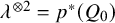. We define $\Sigma ^0\subset \Sigma $ to be the complement of the poles of $\lambda $ .

We consider the homology group $H_1(\Sigma ^0,\mathbb {Z})^-$ . The superscript signifies anti-invariance for the covering involution: we consider only classes satisfying $\sigma _*(\gamma )=-\gamma $ . A calculation shows that $H_1(\Sigma ^0,\mathbb {Z})^-\cong \mathbb {Z}^{\oplus k}$ is free of rank k. Given a basis $(\gamma _1,\ldots ,\gamma _k)\subset H_1(\Sigma ^0,\mathbb {Z})^-$ , we define

(43) $$ \begin{align}z_i=\oint_{\gamma_i} \lambda\in \mathbb{C}.\end{align} $$

As the point $(C,Q_0)\in \mathrm {Quad}(g,m)$ varies, the homology groups $H_1(\Sigma ^0,\mathbb {Z})^-$ fit together to form a local system over $\mathrm {Quad}(g,m)$ . Transporting the basis elements $\gamma _i$ to nearby points, the resulting functions $(z_1,\ldots ,z_k)$ form local coordinates on $\mathrm {Quad}(g,m)$ . In particular, the tangent space at a point of $\mathrm {Quad}(g,m)$ is naturally identified with the cohomology group $H^1(\Sigma ^0,\mathbb {C})^-$ .

The inclusion $i\colon \Sigma ^0\hookrightarrow \Sigma $ defines a natural map

(44) $$ \begin{align} i_*\colon H_1(\Sigma^0,\mathbb{Z})^-\to H_1(\Sigma,\mathbb{Z})^-\end{align} $$

whose image is a finite index subgroup $\Gamma \subset H_1(\Sigma ,\mathbb {Z})^-$ . The intersection form on $H_1(\Sigma ,\mathbb {Z})$ pulls back via $i_*$ to an integral skew-symmetric form $\langle -,-\rangle $ on $H_1(\Sigma ^0,\mathbb {Z})^-$ . The form $\langle -,-\rangle $ then induces a Poisson structure on $\mathrm {Quad}(g,m)$ satisfying

(45) $$ \begin{align}\{z_i,z_j\}=2\pi i \,\langle\gamma_i,\gamma_j\rangle.\end{align} $$

After tensoring with $\mathbb {Q}$ , the kernel of the map (44) is spanned by classes $\pm \beta _i\in H_1(\Sigma ^0,\mathbb {Z})^-$ defined up to sign by the difference of small loops around the two inverse images of an even-order pole of $Q_0$ . The residue of $Q_0$ at such a pole $x_i\in C$ is defined to be the period

(46) $$ \begin{align}\mathrm{Res}_{x_i}(Q_0)=\pm \oint_{\beta_i}\lambda\in \mathbb{C}.\end{align} $$

It is well-defined up to sign and is a Casimir for the above Poisson structure. Fixing these residues locally cuts out a symplectic leaf in $\mathrm {Quad}(g,m)$ of dimension $n=2d$ , where

(47) $$ \begin{align} d=3g-3+ \sum_{i=1}^l \, \bigg\lceil \frac{m_i}{2} \bigg\rceil.\end{align} $$

The tangent space to this leaf is identified with the cohomology group $H^1(\Sigma ,\mathbb {C})^-$ .

The base of our Joyce structure will be the particular symplectic leaf

(48) $$ \begin{align}M=M(g,m)\subset \mathrm{Quad}(g,m)\end{align} $$

obtained by requiring all residues (46) at even-order poles of $Q_0$ to be zero. Note that a pole of $Q_0$ of order 2 with zero residue is in fact a pole of order 1.

Choosing a basis $(\gamma _1,\ldots , \gamma _n)$ for the finite index subgroup $\Gamma \subset H_1(\Sigma ,\mathbb {Z})^-$ gives preferred local coordinates $(z_1,\ldots ,z_n)$ on M defined by formula (43). As in Section 3.1, there are corresponding linear coordinates $(\theta _1,\ldots ,\theta _n)$ on the tangent spaces $T_p M$ obtained by writing a tangent vector in the form $\sum _i \theta _i\cdot \frac {\partial }{\partial z_i}\big |_p$ . We can then consider $(z_i,\theta _j)$ as coordinates on the total space $X=T_M$ . We also introduce the quotient $X^{\#}=X/ (2\pi i)\, \mathbb {Z}^n$ whose local coordinates are $(z_i,e^{\theta _j})$ .

4.2. Isomonodromy flows

To define a Joyce structure on $M,$ we need a system of flows (15). We will construct these by associating to a generic point of the space $X^\#$ a family of differential equations of the form

(49) $$ \begin{align}y"(x)=Q(x,\epsilon) \cdot y(x), \qquad Q(x,\epsilon)=\epsilon^{-2}\cdot {Q_0(x)}+\epsilon^{-1}\cdot Q_1(x) + Q_2(x),\end{align} $$

depending on a parameter $\epsilon \in \mathbb {C}^*$ . In concrete terms, the $Q_i(x)$ are meromorphic functions on C, but more invariantly, $Q_1= Q_1(x) \, d x^{\otimes 2}$ is another meromorphic quadratic differential on C, and $Q_2$ represents a meromorphic projective structure [Reference Allegretti and Bridgeland3]. The required flows (15) will then be given by allowing the point $(C,Q_0)$ to move in the space M and varying the other data $Q_1,Q_2$ so that the generalized monodromy of equation (49) remains constant.

At a point $x_i\in C,$ where $Q_0$ has a pole of order $m_i$ , we will insist that $Q_1$ and $Q_2$ have poles of order at most $\lceil \tfrac {1}{2} m_i\rceil $ . We also allow $Q_1$ and $Q_2$ to have poles at exactly d other points $q_i\in C$ , with d given by (47). At these points, $Q_1$ and $Q_2$ will be required to have the leading-order behavior

(50) $$ \begin{align} Q_1(x)= -\frac{p_i}{x-q_i} + u_i + O(x-q_i), \qquad Q_2(x)=\frac{3}{4(x-q_i)^2} - \frac{r_i}{x-q_i} + v_i +O(x-q_i),\end{align} $$

with $p_i,r_i,u_i,v_i\in \mathbb {C}$ . We will then insist that, for all $\epsilon \in \mathbb {C}^*$ , equation (49) has apparent singularities at the points $x=q_i$ , that is, that the monodromy of the associated linear system is trivial as an element of $\mathrm {PGL}_2(\mathbb {C})$ . This is equivalent to the condition

(51) $$ \begin{align} \left(\epsilon^{-1} p_i+r_i\right)^2=\epsilon^{-2}Q_0(q_i) +\epsilon^{-1} u_i+v_i, \end{align} $$

for all $\epsilon \in \mathbb {C}^*$ (see, e.g., [Reference Bridgeland and Masoero17, Lemma 2.1]), and hence to the equations

(52) $$ \begin{align} p_i^2=Q_0(q_i), \qquad u_i=2p_ir_i, \qquad v_i=r_i^2.\end{align} $$

The first of these relations shows that the pair $(q_i,p_i)$ defines a point of the spectral curve $\Sigma $ .

The condition on the pole orders of $Q_1$ at the points $x_i$ , together with equation (52), ensures that the anti-invariant differential

(53) $$ \begin{align}\theta=-\frac{Q_1(x)\, dx}{2\sqrt{Q_0(x)}}\end{align} $$

on $\Sigma $ has simple poles at the points $(q_i,\pm p_i)$ with residues $\pm \tfrac {1}{2}$ , and no other poles. We will then require that if equation (49) is associated with a point of $X^\#$ with coordinates $(z_i,e^{\theta _j}),$ then

(54) $$ \begin{align} e^{\theta_j}=\exp\left(\oint_{\gamma_j} \theta\right).\end{align} $$

Note that the right-hand side of (54) is well-defined for $\gamma _i\in H_1(\Sigma ^0,\mathbb {Z})^-$ . Indeed, we can lift $\gamma _i$ to an anti-invariant cycle on the curve $\Sigma ^0$ further punctured at the points $(q_i,\pm p_i)$ . Any two ways of doing this differ by a sum of cycles of the form $\delta _i - \sigma ^*(\delta _i)$ , where $\delta _i$ is a small loop around the point $(q_i,p_i)$ . By the residue property of the differential $\theta ,$ such a change affects the integral on the right-hand side of (54) by an element of $2\pi i \mathbb {Z}$ .

It is conjectured in [Reference Bridgeland15, Section 4] that for a generic point of $X^\#$ lying over a point $(C,Q_0)\in M$ , there is a unique equation (49) satisfying the conditions discussed above and (54). In other words, with the given conditions on the poles of $Q_1$ and $Q_2$ , equation (54) determines $Q_1$ uniquely, and then generically $Q_2$ is also uniquely determined by the conditions (52) coming from the assumption that (49) has apparent singularities. It is further claimed in [Reference Bridgeland15, Section 4] that the isomonodromy flows for equation (49) give rise to a Joyce structure on M.

A general construction of these Joyce structures will be given in [Reference Zikidis59] with a different approach involving bundles with connection rather than projective structures with apparent singularities. In this article, we will construct the required Joyce structures in our two examples by direct calculation. This involves computing the isomonodromy flows for equation (49) and rewriting them in the coordinates $(z_i,\theta _j)$ given by (43) and (54).

5.1. Isomonodromic deformations with a reference connection

Consider a meromorphic flat $\mathfrak {g}$ -connection on a rank 2 trivial bundle on $\mathbb {P}^1$ of the form

(55) $$ \begin{align} \nabla_\epsilon:=d-A_0(x)d x-\frac{1}{\epsilon}\Phi(x)d x. \end{align} $$

Here, $d-A_0(x)d x$ is a reference connection, and $\Phi (x)d x$ is a Higgs field, namely, a $\mathfrak {g}$ -valued meromorphic 1-form, and $\epsilon \in \mathbb {C}^*$ . We can relate this to an oper with apparent singularities by performing a singular gauge transformation

(56) $$ \begin{align} g(x)^{-1} \big(d- A(x) d x\big) g(x) = d- \left( \begin{array}{cc}0 & 1 \\ Q(x) & 0 \end{array}\right) d x. \end{align} $$

This can be achieved by taking

(57) $$ \begin{align} g(x) = \left( \begin{array}{cc}A_{12}(x)^{\frac{1}{2}} & 0 \\ 0 & A_{12}(x)^{-\frac{1}{2}}\end{array} \right) \cdot \left( \begin{array}{cc} 1 & 0 \\ \frac{A^\prime_{12}(x)}{2A_{12}(x)}-A_{11}(x) & 1 \end{array} \right). \end{align} $$

The resulting potential is

(58) $$ \begin{align} Q(x)=-\det A(x) +A_{11}(x) \Bigg(\frac{A^\prime_{11}(x)}{A_{11}(x)}-\frac{A^\prime_{12}(x)}{A_{12}(x)}\Bigg)+\frac{3}{4}\Bigg(\frac{A^\prime_{12}(x)}{A_{12}(x)}\Bigg)^2-\frac{A^{\prime \prime}_{12}(x)}{2A_{12}(x)}, \end{align} $$

and the condition $\nabla _\epsilon \Psi =0$ for a flat section becomes the second-order ODE (49) after setting $\Psi =(y(x), y'(x))^T$ .

A meromorphic Higgs field $\Phi (x) dx$ on the Riemann sphere $C=\mathbb {P}^1$ will have the general form

(59) $$ \begin{align} \Phi(x)=-\sum_{j=0}^{d_\infty-1}\Phi_{j+2}^\infty x^j+\sum_{k=1}^n\sum_{j=1}^{d_k+1}\frac{\Phi_j^k}{(x-x_k)^j}. \end{align} $$

Let $\pm y(x)$ be the eigenvalues of $\Phi (x)$ , and $\pm \lambda =\pm y(x)d x$ the eigenvalues of $\Phi (x)d x$ . Away from the poles of $\Phi (x),$ the spectral curve $\Sigma $ is given by the condition $\det (\Phi (x)d x-\lambda \,\mathrm {id})=0$ , that is,

(60) $$ \begin{align} y^2=Q_0(x),\qquad Q_0(x):=-\det\Phi(x)=\frac{1}{2}\mathrm{tr}\Phi(x)^2. \end{align} $$

On the space of Higgs fields, there is a natural R-matrix Lie–Poisson bracket, given by the split rational classical R-matrix [Reference Reyman and Semenov-Tian-Shansky54], [Reference Reyman and Semenov-Tian-Shansky55] (see [Reference Bertola, Harnad and Hurtubise6] for more details in this context). The so-called algebro-geometric Darboux coordinates $(q_i,p_i)$ , where $i=1,\dots ,g(\Sigma )$ , provide a convenient system of coordinates to explicitly parameterize Higgs fields. For our current $\mathfrak {sl}_2$ case, these are defined by

(61) $$ \begin{align} \Phi_{12}(q_i)=0,\qquad \Phi_{11}(q_i)=p_i. \end{align} $$

We see from (60) that $(q_i,p_i)$ are points on the spectral curve $\Sigma $ , namely,

(62) $$ \begin{align} p_i^2=Q_0(q_i). \end{align} $$

We introduce a reference connection through additional parameters $r_i$ , obtained by shifting $p_i\mapsto p_i+\epsilon r_i$ in the Higgs field, analogously to the Painlevé I example in Section 2. In this way, the inhomogeneous term $g^{-1}dg$ in the gauge transformation (56) leads to a double pole of $Q(x) dx^{\otimes 2}$ at the point $x=q_i$ with residue $-p_i-\epsilon r_i$ , and the algebro-geometric Darboux coordinates coincide with the variables $q_i,\,p_i$ of Section 4.2. If we have local monodromy exponents $\mu _k$ , defined by

(63) $$ \begin{align} \mu_k:=\mathrm{Res}_{x=x_k} y(x)d x, \end{align} $$

we will also include in the reference connection parameters $s_k$ defined by shifts $\mu _k\mapsto \mu _k+\left ( s_k+\frac {1}{2}\right )$ . This shifting procedure gives a particular choice of reference connection $A_0$ and immediately gives trivial isomonodromic flows of the form

(64) $$ \begin{align} \widetilde{w}_i=\frac{\partial}{\partial p_i}-\frac{1}{\epsilon}\frac{\partial}{\partial r_i}. \end{align} $$

This problem was solved in [Reference Bertola, Harnad and Hurtubise6] for a general system for which the matrix describing the leading behavior of the Higgs field at a pole is diagonalizable with distinct eigenvalues. This genericity assumption is not satisfied in the examples corresponding to Painlevé I and III $_3$ , so that, in Section 6, we will use a slightly different set of coordinates.

We will denote the spectral invariants as $t_{j,k}$ and $H_{j,k}$ , with the $t_{j,k}$ being Casimir elements, with $k=1,\dots ,n$ indexing the poles $x_k$ , and $j=1,\dots d_k$ . The spectral invariants are given by

(65) $$ \begin{align} t_{j,k}:=-\mathrm{Res} (x-x_k)^jy(x)d x,\quad H_{j,k}:=-\mathrm{Res}_{x=x_k}\frac{y(x)d x}{j(x-x_k)^j},\\[-38pt]\nonumber \end{align} $$

(66) $$ \begin{align} t_{0,k}:=x_k,\qquad H_{0,k}:=\frac{1}{2} \mathrm{Res}_{x=x_k} \mathrm{tr} \Phi(x)^2 dx. \end{align} $$

For the case of a singular point that has been fixed at infinity,

(67) $$ \begin{align} t_{j,\infty}:=-\mathrm{Res} x^{-j}y(x)d x,\qquad H_{j,\infty}:=-\frac{1}{j}\mathrm{Res}_{x=\infty} x^{j} y(x)d x. \end{align} $$

In the usual setting of isomonodromic deformations without a reference connection, $t_{j,k}$ are isomonodromic times, whose flows are generated by the Hamiltonians $H_{j,k}$ through the R-matrix Poisson bracket. In our present context, these are all isomonodromic times: choosing as coordinates the r’s, q’s, H’s, and t’s, and regarding $p_i$ as functions of the other variables through (62), the flows $\widetilde {w}_i$ can be written as

(68) $$ \begin{align} \widetilde{w}_i=\sum_{k=1}^n\sum_{j=1}^{d_k}\frac{\partial H_{j,k}}{\partial p_i}\bigg|_{q_i}\, \frac{\partial}{\partial H_{j,k}}-\frac{1}{\epsilon}\frac{\partial}{\partial r_i}, \end{align} $$

where the subscript denotes partial derivatives with the variables $q_i$ fixed. By rescaling and taking linear combinations of the $\widetilde {w}_i$ ’s, the flows can be brought to the form $w_{j,k}=\frac {\partial }{\partial H_{j,k}}+\cdots $ . The other isomonodromic deformation equations can be obtained from the compatibility of the linear systems

(69) $$ \begin{align} \begin{cases} \partial_x \Psi(x)=A(x)\Psi(x), \\ \partial_{t_{j,k}} \Psi(x)=B_{j,k}(x)\Psi(x),\qquad j=1,\dots,d_k,\,k=1,\dots,n \end{cases} \end{align} $$

and are given by

(70) $$ \begin{align} \partial_{t_{l,k}}A-\partial_x B_{l,k}+[A,B_{l,k}]=0,\qquad \partial_{t_{l,k}}B_{j,l}-\partial_{t_{j,k}}B_{l,k}+[B_{j,l},B_{l,k}]=0, \end{align} $$

with the matrices $B_{j,k}$ themselves being fixed by the consistency conditions.

In fact, the isomonodromic equations can be obtained in a uniform manner as the compatibility of the system

(71) $$ \begin{align} \begin{cases} \partial_x \Psi(x)=A(x)\Psi(x), \\ \partial_{t_{j,k}} \Psi(x)=B_{j,k}(x)\Psi(x),& j=1,\dots,d_k,\,k=1,\dots,n, \\ \partial_{r_i}\Psi(x)=0, & i=1,\dots, g(\Sigma). \end{cases} \end{align} $$

6.1. Higgs field and quadratic differential

Take $q,t\in \mathbb {C}^*$ and $p\in \mathbb {C}$ and consider the meromorphic Higgs field $\Phi =\Phi (x) \, d x$ on the trivial rank 2 vector bundle over $\mathbb {P}^1$ defined by

(72) $$ \begin{align} \Phi(x)=\frac{1}{x^2}\left(\begin{array}{cc} 0 & -q \\ 0 & 0 \end{array} \right)+\frac{1}{x}\left(\begin{array}{cc} pq & 1 \\ -q^{-1} & -pq \end{array} \right)+ \left(\begin{array}{cc} 0 & 0 \\ t & 0 \end{array} \right). \end{align} $$

Note that $\Phi $ has double poles at $x=0$ and $x=\infty $ with nilpotent leading-order behavior. Thus, $x=0$ and $x=\infty $ are irregular singularities of the connection $d-\Phi $ of Poincaré rank $\frac {1}{2}$ .

Then matrix $\Phi (x)$ is a Lax matrix for the Painlevé III $_3$ equation (see, e.g., [Reference Gavrylenko and Lisovyy39, Section 2])

(73) $$ \begin{align} \frac{d^2q}{d t^2}=\frac{1}{q}\left(\frac{d q}{d t} \right)^2-\frac{1}{t}\frac{d q}{d t}+\frac{2q^2}{t}-\frac{2}{t^2}, \end{align} $$

in the sense that (73) describes isomonodromic deformation of the connection $d-\Phi $ .

A slight complication in this case is that the poles are branch points of the spectral curve, so that one would need to modify the connection along the lines of [Reference Gavrylenko and Lisovyy39, Section 2.1] in order for equation (65) to hold. We will circumvent this issue by introducing the parameter H simply as

(74) $$ \begin{align} H=\mathrm{Res}_{x=0} \left(\frac{x}{2} \mathrm{tr}\Phi(x)^2\,dx\right)=p^2q^2-tq-q^{-1}. \end{align} $$

Since $t\in \mathbb {C}^*$ , the spectral invariant

(75) $$ \begin{align} \frac{1}{2} \mathrm{tr}(\Phi^2)= Q_0(x) \, dx^{\otimes 2}= \frac{1}{x^2}\left(tx+H +x^{-1}\right) dx^{\otimes 2}\end{align} $$

is a meromorphic quadratic differential on $\mathbb {P}^1$ with poles of order 3 at the points $x=0$ and $x=\infty $ . Conversely, any quadratic differential on $\mathbb {P}^1$ with two poles of order 3 and no other poles can be put in the form (75) by applying an automorphism of $\mathbb {P}^1$ .

The base M of our Joyce structure will parameterize differentials of the form (75) which have simple zeros. Thus,

(76) $$ \begin{align} M=\big\{(t,H)\in \mathbb{C}^2: t(H^2-4t)\neq 0\big\}.\end{align} $$

One exceptional feature in this example is that every differential of the form (75) is preserved by a unique nontrivial automorphism of $\mathbb {P}^1$ , namely, $x\mapsto (tx)^{-1}$ . In more abstract language, the stack $\mathrm {Quad}(g,m)$ of quadratic differentials has generic stabilizer $\mathbb {Z}_2$ in this example [Reference Bridgeland and Smith18, Section 2.7].

We will construct a Joyce structure on M by considering isomonodromic flows for meromorphic connections of the form

(77) $$ \begin{align} \nabla_\epsilon= d-A_\epsilon (x)d x, \qquad A_\epsilon (x)=A_\infty(x)+\frac{1}{\epsilon}\, \Phi(x), \end{align} $$

where $A_\epsilon (x)$ is obtained from $\Phi (x)$ by the shift $p\mapsto p+\epsilon rq^{-1}$ . Explicitly,

(78) $$ \begin{align} \nabla_\epsilon=d- \left(\begin{array}{cc} r & 0 \\ 0 & -r \end{array} \right)\frac{d x}{x}-\frac{1}{\epsilon}\left(\begin{array}{cc} pq & 1-qx^{-1} \\ tx-q^{-1} & -pq \end{array} \right)\frac{d x}{x}. \end{align} $$

We view this connection as being parameterized by $\epsilon \in \mathbb {C}^*$ together with the variables $(t,H,q,r)$ , with p defined implicitly by (74).

6.2. Extended isomonodromic flows

Let us fix $\epsilon \in \mathbb {C}^*$ . If we move the point $(t,H)\in M,$ we can vary $q=q(t,H)$ and $r=r(t,H)$ in such a way that the generalized monodromy of the connection (78) is constant. The following result gives an explicit basis for the resulting two-dimensional space of isomonodromic flows.

Proposition 1. The generalized monodromy of (78) is preserved by the vector fields

(79) $$ \begin{align} w_1=t\frac{\partial}{\partial t}+\frac{2pq^2}{\epsilon }\frac{\partial}{\partial q}+2qr\frac{\partial}{\partial q}-\frac{1}{2\epsilon pq^2}(2rq^2 t-2r+q^2t)\frac{\partial}{\partial r}, \\[-38pt]\nonumber \end{align} $$

(80) $$ \begin{align} w_2=\frac{\partial}{\partial H}-\frac{1}{2\epsilon p q}\frac{\partial}{\partial r}. \end{align} $$

Proof. Let us first consider the connection $d-A_\epsilon (x) dx$ as being a function of the variables $(t,q,p,r)$ , with H determined by (74). We can describe isomonodromic deformations of this connection with parameter t as the compatibility conditions of the linear systems

(81) $$ \begin{align} \partial_x Y(x)=A_\epsilon(x)Y(x), \qquad \partial_t Y(x)=B_\epsilon(x)Y(x). \end{align} $$

The consistency condition

(82) $$ \begin{align} \partial_t A_\epsilon(x)-\partial_xB_\epsilon(x)+[A_\epsilon(x),B_\epsilon(x)]=0 \end{align} $$

requires that we take

(83) $$ \begin{align} B_\epsilon(x) =\frac{1}{\epsilon t}\left(\begin{array}{cc} pq+\epsilon r & 1 \\ 0 & -pq-\epsilon r \end{array} \right)+ \frac{x}{\epsilon}\left(\begin{array}{cc} 0 & 0 \\ 1 & 0 \end{array} \right) \end{align} $$

and gives the equations

(84) $$ \begin{align} t\frac{d q}{d t}=\frac{2pq^2}{\epsilon}+2qr, \qquad t\frac{d }{d t}(pq+\epsilon r)=\frac{1}{\epsilon}\left(q t-q^{-1} \right). \end{align} $$

Differentiating (74) then gives

(85) $$ \begin{align} \frac{dH}{dt}=\frac{2r-q^2t(2r+1)}{tq}-2pq\epsilon\, \frac{dr}{dt}. \end{align} $$

Equation (84) does not uniquely determine an isomonodromic flow because everything depends only on the combination $pq+\epsilon r$ , meaning that both $\partial _x-A_\epsilon (x)$ and $\partial _t-B_\epsilon (x) $ , and in particular the monodromy of $\nabla _\epsilon $ , are constant along the vector field

(86) $$ \begin{align} \widetilde{w_2}=\frac{\partial}{\partial r}-\frac{\epsilon}{q}\frac{\partial}{\partial p}. \end{align} $$

To fix this ambiguity, we impose that $\frac {d H}{d t}=0$ by adding a multiple of the vector field $\tilde {w}_2$ .

We now rewrite the flows in the variables $(t,H,q,r)$ , with p determined by (74). The first flow becomes

(87) $$ \begin{align} t\frac{d q}{d t}=\frac{2pq^2}{\epsilon}+2qr, \qquad t\frac{d r}{d t}=\frac{2 r-q^2 t (2 r +1)}{2 p q^2 \epsilon }, \end{align} $$

which is generated by the vector field $w_1$ . Moreover, (86) becomes

(88) $$ \begin{align} \widetilde{w_2}=\frac{\partial}{\partial r}-2\epsilon pq \frac{\partial}{\partial H}, \end{align} $$

which is equivalent to $w_2$ by a simple rescaling.

Remark 2. The combination $w_1-qtw_2$ gives the flow

(89) $$ \begin{align} t\frac{dq}{dt}=\frac{2pq^2}{\epsilon}+2qr,\qquad t\frac{dp}{dt}=-\frac{2p^2q-t+q^{-2}}{\epsilon}+\frac{r \left(-4 p^2 q^3+2 q^2 t-2\right)}{2 p q^3},\qquad t\frac{dH}{dt}=-tq. \end{align} $$

When $r=0,$ this reproduces the usual Painlevé flow defined by the Hamiltonian H and the symplectic form $tdq\wedge dp$ . In contrast to what happens in the usual treatment of Painlevé equations, however, in the presence of a reference connection, the flow in t can be normalized so that H is conserved. However, since q is unaffected by the flow $w_2$ , irrespective of how we normalize the flow, the second-order isomonodromy equation for q is still the ( $\epsilon $ -deformed) Painlevé III $_3$ equation

(90) $$ \begin{align} \frac{d^2 q}{d t^2}=\frac{1}{q}\left(\frac{d q}{d t} \right)^2-\frac{1}{t}\frac{d q}{d t}+\frac{1}{\epsilon^2}\left(\frac{2q^2}{t}-\frac{2}{t^2}\right). \end{align} $$

This phenomenon was observed in the Painlevé I example in [Reference Dunajski and Moy31, Section 6.1].

6.3. Spectral curve and its homology

Let us fix a point $(t,H)\in M$ . The spectral curve $\Sigma $ is a smooth curve of genus one which is a double cover $p\colon \Sigma \to \mathbb {P}^1$ branched over four points of $\mathbb {P}^1$ . We denote by $\sigma \colon \Sigma \to \Sigma $ the covering involution. The branch points of p include the points $0,\infty \in \mathbb {P}^1$ , and we will also write $0,\infty \in \Sigma $ for the unique points of $\Sigma $ lying over them.

The open subset $\Sigma ^0\subset \Sigma $ is the complement $\Sigma ^0=\Sigma \setminus \{0,\infty \}$ . This subset can be identified with the set of points $(x,y)\in \mathbb {C}^*\times \mathbb {C}$ satisfying

(91) $$ \begin{align} y^2=Q_0(x)=\frac{t}{x}+\frac{H}{x^2}+\frac{1}{x^3}. \end{align} $$

The projection is then $p(x,y)=x$ and the covering involution is $\sigma (x,y)=(x,-y)$ .

Lemma 1. The inclusion $i\colon \Sigma ^0\hookrightarrow \Sigma $ induces an embedding of anti-invariant homology groups

(92) $$ \begin{align}i_*\colon H_1(\Sigma^0,\mathbb{Z})^-\hookrightarrow H_1(\Sigma,\mathbb{Z})^-=H_1(\Sigma,\mathbb{Z})\end{align} $$

whose image has index 2.

In what follows, we will fix a basis $(\gamma _1,\gamma _2)$ for the group $H_1(\Sigma ^0,\mathbb {Z})^-$ . The intersection form on $H_1(\Sigma ,\mathbb {Z})$ pulls back along $i_*$ to give a skew-symmetric pairing on $H_1(\Sigma ^0,\mathbb {Z})^-$ . Since the image of $i_*$ has index 2, we can order our basis so that $\langle \gamma _1,\gamma _2\rangle =2$ .

6.4. Forms and periods

By the gauge transformation (56), we can rewrite (78) as a scalar equation of the form (49). In this case, we have $Q_0(x)$ as in (75) above, and

(93) $$ \begin{align} Q_1(x)=-\frac{pq^2}{x^2(x-q)}+\frac{2pqr}{x^2}, \qquad Q_2(x)=\frac{3}{4(x-q)^2}-\frac{x+rq}{x^2(x-q)}+\frac{r^2}{x^2}. \end{align} $$

As in Section 4, we introduce meromorphic differentials on $\Sigma $ by the expressions

(94) $$ \begin{align}\lambda = y\, d x, \qquad \theta=-\frac{Q_1(x) \, dx }{2\sqrt{Q_0(x)} }.\end{align} $$

The Seiberg–Witten differential $\lambda $ has double poles at the points $0,\infty \in \Sigma $ , and no other poles. The differential $\theta $ has simple poles at the points $(q,\pm p)$ with residues $\pm \tfrac {1}{2}$ , respectively, and no other poles. We introduce the periods

(95) $$ \begin{align}z_i=\oint_{\gamma_i} \lambda, \qquad \theta_i=\oint_{\gamma_i} \theta.\end{align} $$

Note that the expressions $\theta _i$ are only well-defined up to the addition of integer multiples of $2\pi i$ . To specify them, we must lift the cycles $\gamma _i$ to the complement $\Sigma ^*=\Sigma ^0\setminus \{(q,\pm p)\}$ . We can always do this so that the resulting elements $\gamma ^*_i\in H_1(\Sigma ^*,\mathbb {Z})$ are anti-invariant. Since $\theta $ has residues $\pm \tfrac {1}{2}$ at the points $(q,\pm p)$ , taking different lifts changes the result by a multiple of $2\pi i$ .

Let us set $s=\log (t)$ and take $(s,H)$ as local coordinates on the base M. There are corresponding linear coordinates $(\theta _s,\,\theta _H)$ on the fibers of the projection $\pi \colon X=T_M\to M$ defined by the relation

(96) $$ \begin{align} \theta_s\, \frac{\partial }{\partial s} +\theta_H\, \frac{\partial }{\partial H} =\theta_1\, \frac{\partial }{\partial z_1} +\theta_2\, \frac{\partial }{\partial z_2}. \end{align} $$

Introduce the differentials

(97) $$ \begin{align}\omega=\frac{\partial \lambda}{\partial H} =\frac{dx}{2x^2y}, \qquad \beta=\frac{\partial \lambda}{\partial s} =\frac{t\, dx}{2x y}.\end{align} $$

Then $\omega $ is a holomorphic differential on $\Sigma $ , and $\beta $ has a pole of order 2 with vanishing residue at the branch point $x = \infty $ and no other poles. We denote the corresponding periods by $\omega _{i}$ and $\beta _i$ , respectively. There is an obvious relation

(98) $$ \begin{align}dz_i=\frac{\partial z_i}{\partial s} \, ds+\frac{\partial z_i}{\partial H} \, dH=\beta_i \, ds+\omega_i \, dH,\end{align} $$

and using (96), we get

(99) $$ \begin{align}\theta_i=\beta_i\theta_s+\omega_i\theta_H.\end{align} $$

6.5. Computation of periods

In this section, we use the Riemann bilinear relations to give explicit expressions for $\theta _s$ and $\theta _H$ .

Lemma 2. There are formulas

(100) $$ \begin{align}\theta_s=\frac{1}{2} \int_{(q,-p)}^{(q,p)} \frac{dx}{2x^2y}, \qquad \theta_H= -\frac{1}{2} \int_{(q,-p)}^{(q,p)} \frac{t\, dx}{2xy}-2pqr.\end{align} $$

Proof. Note that $y=\sqrt {Q_0(x)}$ is a uniformizing parameter at the point $\infty \in \Sigma $ . We denote by $x^{1/2}$ the choice of square root near this point for which $y\simeq t^{1/2}x^{-1/2}$ . The differentials introduced above have leading-order behavior

(101) $$ \begin{align} \omega=\frac{d x}{2t^{1/2}x^{3/2}}+O\left(\frac{d x}{x^{5/2}} \right), \qquad \beta=\frac{t^{1/2} d x}{2x^{1/2}}+O\left(\frac{d x}{x^{3/2}} \right),\\[-38pt]\nonumber \end{align} $$

(102) $$ \begin{align}\qquad \theta=-\frac{pqr \, dx}{t^{1/2}x^{3/2}}+O\left(\frac{d x}{x^{5/2}} \right). \end{align} $$

The Riemann bilinear relations for meromorphic differentials (see Proposition 3.4.1 in [Reference Bertola7], a direct consequence, e.g., of equations 3.0.1 and 3.0.2 in [Reference Farkas, Kra, Farkas and Kra33]) give

(103) $$ \begin{align}\omega_1\beta_{2}-\omega_2\beta_{1} = 2\pi i \cdot \langle\gamma_1,\gamma_2\rangle\cdot \mathrm{Res}_{x=\infty}\left( \beta\int^x\omega\right). \end{align} $$

Note that although this formula is usually given in the case that the cycles $\gamma _1,\gamma _2\in H_1(\Sigma ,\mathbb {Z})$ satisfy $\langle \gamma _1,\gamma _2\rangle =1$ , the case of an arbitrary pair of linearly independent cycles follows immediately from this. Note also that the form $dx/x$ has residue $-2$ at the point $\infty \in \Sigma $ . Using $\langle \gamma _1,\gamma _2\rangle =2$ and the expressions (101), we then get

(104) $$ \begin{align}\langle\omega,\beta\rangle:=\omega_1\beta_{2}-\omega_2\beta_{1} =4\pi i.\end{align} $$

We can write similar expressions

(105) $$ \begin{align}\langle\omega,\theta\rangle :=\omega_1\theta_2-\omega_2\theta_1 = 4\pi i \sum_{x_i\in \{(q,\pm p)\}}\mathrm{Res}_{x=x_i}\left(\theta\int^x\omega\right) =2\pi i \int_{(q,-p)}^{(q,p)}\omega,\\[-38pt]\nonumber\end{align} $$

(106) $$ \begin{align} \langle\beta,\theta\rangle:=\beta_{1}\theta_2-\beta_{2}\theta_1 = 4\pi i \sum_{x_i\in\{(q,\pm p),\infty\}}\mathrm{Res}_{x=x_i}\left(\theta\int^x\beta \right)=2\pi i \int_{(q,-p)}^{(q,p)}\beta+8\pi i pqr. \end{align} $$

Using (99), we then have

(107) $$ \begin{align} 2\pi i \int_{(q,-p)}^{(q,p)}\omega= \langle\omega,\theta\rangle=\theta_s\langle\omega,\beta\rangle=4\pi i\theta_s,\\[-38pt]\nonumber \end{align} $$

(108) $$ \begin{align} 2\pi i\int_{(q,-p)}^{(q,p)}\beta+8\pi i pqr=\langle\beta,\theta\rangle=\theta_H\langle\beta,\omega\rangle=-4\pi i\theta_H, \end{align} $$

and comparing with (97) gives the result.

Recall from (45) that the Poisson structure on M is defined by the condition

(109) $$ \begin{align}\{z_1,z_2\}=2\pi i \, \langle\gamma_1,\gamma_2\rangle=4\pi i.\end{align} $$

Inverting this gives the symplectic form

(110) $$ \begin{align} \Omega_0=-\frac{1}{4\pi i} \cdot dz_1\wedge dz_2 = \frac{1}{4\pi i} (\omega_1\beta_{2}-\omega_2\beta_{1})\cdot ds\wedge dH=ds\wedge dH,\end{align} $$

where we used (98) and (104).

6.6. Abelian holonomy map

Denote by $\Xi $ the change of coordinates $(s,H,q,r)\mapsto (s,H,\theta _s,\theta _H)$ . Applying the chain rule to Lemma 2 gives

(111) $$ \begin{align} \Xi_*\left(\frac{\partial}{\partial s} \right)=\frac{\partial}{\partial s}-t\kappa_3 \frac{\partial}{\partial\theta_s}+\left( -\frac{t}{4} \int_{(q,-p)}^{(q,p)} \frac{dx}{xy}+t^2\kappa_2 -\frac{rt}{p} \right)\frac{\partial}{\partial\theta_H}, \\[-38pt]\nonumber\end{align} $$

(112) $$ \begin{align} \Xi_* \Bigg(\frac{\partial}{\partial H}\Bigg)=\frac{\partial}{\partial H}-\kappa_4 \frac{\partial}{\partial \theta_s} + \Bigg(t \kappa_3 -\frac{r}{qp}\Bigg)\frac{\partial}{\partial \theta_H},\\[-38pt]\nonumber\end{align} $$

(113) $$ \begin{align}\Xi_* \Bigg(\frac{\partial}{\partial q}\Bigg)=\frac{1}{2q^2p} \frac{\partial}{\partial \theta_s} +\frac{2r-2trq^2-tq^2}{2pq^3}\frac{\partial}{\partial \theta_H},\qquad \Xi_* \Bigg(\frac{\partial}{\partial r}\Bigg)=-2qp \frac{\partial}{\partial \theta_H},\end{align} $$

where we introduced

(114) $$ \begin{align}\kappa_i:=\frac{1}{8}\int_{(q,-p)}^{(q,p)} \frac{dx}{x^i y^3},\qquad i=2,3,4.\end{align} $$

Inverting the relations (112) and (113) gives

(115) $$ \begin{align} \Xi_*^{-1} \Bigg(\frac{\partial}{\partial \theta_s}\Bigg)={2q^2p} \frac{\partial}{\partial q} +\frac{2r-2trq^2-tq^2}{2pq^2}\frac{\partial}{\partial r},\qquad \Xi_*^{-1} \Bigg(\frac{\partial}{\partial \theta_H}\Bigg)=-\frac{1}{2qp}\frac{\partial}{\partial r}.\end{align} $$

Fix a point $(t,H)\in M$ and a basis $(\gamma _1,\gamma _2)\in H^1(\Sigma ^0,\mathbb {Z})^-$ as above.

Lemma 3. The map

(116) $$ \begin{align} \big\{(q,p)\in (\mathbb{C}^*)^2: p^2=Q_0(q)\big\}\times \big\{r\in \mathbb{C}\big\}\to \big\{(e^{\theta_1},e^{\theta_2})\big\}\in (\mathbb{C}^*)^2\end{align} $$

defined by equations (93)–(95) is an unramified double cover.

Proof. The degree 0 divisor $(q,p)-\infty $ on $\Sigma $ defines a line bundle whose local sections are meromorphic functions on $\Sigma $ with a zero at $(q,p)$ and at worst a simple pole at $\infty $ . Consider the form

(117) $$ \begin{align} \theta'=\theta+\frac{dx}{2(x-q)} \end{align} $$

on $\Sigma $ . It has a simple pole at $(q,p)$ with residue $+1$ , a simple pole at $\infty $ with residue $-1$ , and no other poles. It follows that $\partial =d-\theta '$ defines a holomorphic connection on L. Since $\theta '-\theta $ is pulled back from $\mathbb {P}^1$ , the form $\theta '$ has the same periods as $\theta $ . Thus, the monodromy of the connection $(L,\partial )$ around the cycle $\gamma _i\in H_1(\Sigma ^0,\mathbb {Z})^-$ is given by multiplication by $\exp (\theta _i)\in \mathbb {C}^*$ .

Suppose there are three points $(q_i,p_i,r_i)$ with $i=1,2,3$ in the source of (116) which are mapped to the same point. Since the cycles $\gamma _1,\gamma _2$ span an index 2 subgroup of $H_1(\Sigma ,\mathbb {Z})$ , at least two of the points (without loss of generality, corresponding to $i=1,2$ ) must correspond to line bundles with connection $(L_i,\partial _i)$ which have identical monodromy around all cycles in $H_1(\Sigma ,\mathbb {Z})$ . The abelian Riemann–Hilbert correspondence tells us that such line bundles with connection $(L_i,\nabla _i)$ are isomorphic. But it is a well-known fact (easily proved using the Riemann–Roch theorem) that the line bundles $L_i$ defined by different points $(q_i,p_i)\in \Sigma $ are all non-isomorphic. So we conclude that $(q_1,p_1)=(q_2,p_2)$ . But formulas (99) and (100) then imply that also $r_1=r_2$ . Indeed, $\omega _1,\omega _2\in \mathbb {C}^*$ do not lie on the same ray, so changing r cannot move both $\theta _i$ by an imaginary number.

The derivative of the map (116) is computed by (111) and (112) together with (99) and is everywhere invertible. Thus, (116) is a finite unramified cover of degree at most 2. Now it is easy to check that our map is invariant under the involution

(118) $$ \begin{align} (q,p,r)\mapsto \left((qt)^{-1},-tpq^2 ,-(r+\tfrac{1}{2})\right), \end{align} $$

and this involution is moreover fixed-point free. Therefore, the map is a double cover.

6.7. Isomonodromic flows in new coordinates

We now write the isomonodromic flows in coordinates $(s,H,\theta _s,\theta _H)$ .

Proposition 1. The push-forward of the isomonodromic flows along $\Xi $ can be written in the form

(119) $$ \begin{align} \Xi_*(w_1)=\frac{\partial}{\partial s}+\frac{1}{\epsilon}\frac{\partial}{\partial\theta_s}+\frac{\partial^2K}{\partial\theta_s\partial\theta_H}\frac{\partial}{\partial\theta_s}-\frac{\partial^2K}{\partial\theta_s^2}\frac{\partial}{\partial\theta_H}, \\[-38pt]\nonumber\end{align} $$

(120) $$ \begin{align} \Xi_*(w_2)=\frac{\partial}{\partial H}+\frac{1}{\epsilon}\frac{\partial}{\partial\theta_H}+\frac{\partial^2K}{\partial\theta_H^2}\frac{\partial}{\partial\theta_s}-\frac{\partial^2K}{\partial\theta_s\partial\theta_H}\frac{\partial}{\partial\theta_H}, \end{align} $$

where $K\colon X^\#\to \mathbb {C}$ is a single locally-defined function.

Proof. Formulas (79) and (80) for the isomonodromic flows and the relations (111)–(113) give

(121) $$ \begin{align} \Xi_*(w_1)=\frac{\partial}{\partial s}+\frac{1}{\epsilon}\frac{\partial}{\partial \theta_s}+b\frac{\partial}{\partial \theta_s} - a\frac{\partial}{\partial \theta_H}, \\[-38pt]\nonumber\end{align} $$

(122) $$ \begin{align} \Xi_*(w_2)=\frac{\partial}{\partial H}+\frac{1}{\epsilon}\frac{\partial}{\partial \theta_H}+c\frac{\partial}{\partial \theta_s} -b\frac{\partial}{\partial \theta_H},\end{align} $$

where we introduced

(123) $$ \begin{align} a=\frac{t}{4} \int_{(q,-p)}^{(q,p)} \frac{dx}{xy}-t^2\kappa_2+\frac{2rt}{p}+\frac{2r^2(tq^2-1)}{pq^2}, \qquad b=\frac{r}{qp}-t\kappa_3,\qquad c=-\kappa_4. \end{align} $$

Using (115), we find that

(124) $$ \begin{align} \frac{\partial b}{\partial \theta_s}=\frac{\partial a}{\partial \theta_H}, \qquad \frac{\partial c}{\partial \theta_s}=\frac{\partial b}{\partial \theta_H}. \end{align} $$

This implies the existence of a single locally-defined function K such that

(125) $$ \begin{align} \frac{\partial^2 K}{\partial \theta_s^2}=a , \qquad \frac{\partial^2 K}{\partial \theta_s \partial \theta_H}=b,\qquad \frac{\partial^2 K}{\partial \theta_H^2}=c,\end{align} $$

and the result follows.

Applying the operators (115) to the expressions (123) gives

(126) $$ \begin{align}\frac{\partial^3 K}{\partial\theta_s^3} =-\frac{3 t^2}{2 p^2}+qt +\frac{2 r t}{p^2q^2} \left(3-3 tq^2+2 p^2q^3\right)+\frac{2 r^2 }{p^2q^4}\left(-1+2Hq+10tq^2+2Htq^3 -t^2 q^4 \right), \\[-38pt]\nonumber\end{align} $$

(127) $$ \begin{align} \frac{\partial^3 K}{\partial \theta_s^2 \partial \theta_H}=-\frac{t}{p^2 q}+\frac{2r}{p^2q^3}\left(1- tq^2 \right), \qquad \frac{\partial^3 K}{\partial \theta_s \partial \theta_H^2}=-\frac{1}{2q^2p^2}, \qquad \frac{\partial^3 K}{\partial \theta_H^3}=0.\end{align} $$

6.8. Plebański function

While K is the generating function for the flows $\Xi _*(w_i)$ , it is not a simple function of our original variables $(p,q,t,r)$ . In fact, integrating the above equations, it is easy to see that K will be expressed in terms of complicated combinations of elliptic functions.

Theorem 6.1. In the coordinates $(z_1,z_2,\theta _1,\theta _2),$ the isomonodromy flows take the form

(128) $$ \begin{align} \frac{\partial}{\partial z_i}+\frac{1}{\epsilon}\cdot \frac{\partial}{\partial\theta_i}+4\pi i\cdot \frac{\partial^2 W}{\partial\theta_i\partial\theta_1}\cdot \frac{\partial}{\partial\theta_2}- 4\pi i\cdot\frac{\partial^2 W}{\partial\theta_i\partial\theta_2}\cdot \frac{\partial}{\partial\theta_1}, \end{align} $$

where the Plebański function W is given by

(129) $$ \begin{align} W=\frac{pq}{6(H^2-4t)}\big(tq+(H+6tq)r+(6H+12tq)r^2+8p^2q^2r^3\big).\end{align} $$

Proof. Let us temporarily introduce variables $u_1=H\cdot \sqrt {4\pi i}$ and $u_2=s\cdot \sqrt {4\pi i}$ . We also set $\phi _1=\theta _H\cdot \sqrt {4\pi i}$ and $\phi _2=\theta _s\cdot \sqrt {4\pi i}$ . Then, by (110), the change of variables $(z_1,z_2) \mapsto (u_1,u_2)$ is symplectic. Dividing (119) and (120) by $\sqrt {4\pi i}$ and making the trivial change from $(s,H)\mapsto (u_1,u_2)$ shows that the isomonodromy flows are spanned by the vector fields

(130) $$ \begin{align}\frac{\partial}{\partial u_i}+\frac{1}{\epsilon}\cdot \frac{\partial}{\partial\phi_i}+4\pi i\cdot \frac{\partial^2 K}{\partial\phi_i\partial\phi_1}\cdot \frac{\partial}{\partial\phi_2}- 4\pi i \cdot \frac{\partial^2 K}{\partial\phi_i\partial\phi_2}\cdot \frac{\partial}{\partial\phi_1}.\end{align} $$

Applying [Reference Bridgeland and Masoero17, Proposition 4.2] to the variable change $(z_1,z_2) \mapsto (u_1,u_2)$ then gives the flows in the form (128). Note that the resulting function W is only well-defined up to the addition of linear functions in the $\theta $ variables.

According to [Reference Bridgeland and Masoero17, Proposition 4.2], the functions K and W differ by a cubic function of the $\theta $ variables. In particular, the fourth derivatives of K and W in the $\theta $ variables necessarily coincide. Now, the fourth derivatives of K can be computed by applying the operators (115) to (126) and (127), and it is then possible to check that these coincide with the fourth derivatives of the expression $\tilde {W}$ on the right-hand side of (129. Thus, $\tilde {W}$ can differ from W by at most quartic functions of the $\theta $ variables. But the second derivatives of W in the $\theta $ variables are necessarily periodic in $\theta $ . Since $\tilde {W}$ is also periodic in $\theta ,$ it must coincide with W up to the addition of linear functions in the $\theta $ variables, which is the required statement, since W was only well-defined up to this indeterminacy.

We can directly check the properties (18)–(20) of the Plebański function. From the change of variables between the coordinates $(z_1,z_2,\theta _1,\theta _2)$ and $(t,H,q,r)$ , it is easy to see that there is an equality of vector fields on $X^\#$

(131) $$ \begin{align} E:=z_1\frac{\partial}{\partial z_1}+ z_2\frac{\partial}{\partial z_1}=4\frac{\partial}{\partial s}+2H\frac{\partial}{\partial H} -2q\frac{\partial}{\partial q}.\end{align} $$

Thus, (19) is the statement that W is homogeneous of weight $-1$ under rescaling $(t,H,q,r)$ with weights $(4,2,-2,0)$ . Note that, by (74), this also involves rescaling the implicit variable p with weight $3$ . Secondly, (100) shows that the map $(q,p)\mapsto (q,-p)$ changes the sign of $(\theta _1,\theta _2)$ . Thus, (18) corresponds to the fact that W is an odd function of the variable p. Finally, W has the periodicity property (20) because, by Lemma 3, it is a function of $(z_1,z_2,e^{\theta _1},e^{\theta _2})$ .

6.9. Plebański function near $\theta =0$

We would like to understand the behavior of the potentials W and K near the zero section $M\subset T_M$ defined by $\theta _t=\theta _H=0$ . This is not completely straightforward, because the potentials are expressed in the variables $(t,H,q,r)$ rather than $(t,H,\theta _t,\theta _H)$ . To study this limit, we will first uniformize the spectral curve $\Sigma $ defined by (91). Observe that if we introduce

(132) $$ \begin{align} X=tx+\tfrac{1}{3}H,\qquad Y=2tx^2y, \end{align} $$

then $\Sigma $ is brought into the standard Weierstrass form

(133) $$ \begin{align} Y^2=4X^3-g_2X-g_3,\qquad g_2=\frac{1}{3}\left(4H^2-12t\right),\qquad g_3=\frac{4H}{27}\left(9t-2H^2 \right). \end{align} $$

It can then be uniformized by writing

(134) $$ \begin{align} X=\wp(u),\qquad Y=\wp'(u), \end{align} $$

with $\wp (u)$ the Weierstrass $\wp $ -function. The differentials $\omega ,\,\beta $ are given by

(135) $$ \begin{align} \omega=\frac{d x}{2x^2y}=\frac{d X}{Y}=d u,\qquad \beta=\frac{t d x}{2xy}=xt\omega=\frac{1}{3}\left(3\wp(u)-H\right)du. \end{align} $$

Denote by $v\in \mathbb {C}$ a point corresponding to the point $(q,p)\in \Sigma $ , so that

(136) $$ \begin{align} q=\frac{1}{3t}\left(3\wp(v)-H \right),\qquad p=\frac{9t\wp'(v)}{2\left(3\wp(v)-H \right)^2}. \end{align} $$

Then we have

(137) $$ \begin{align} \theta_s=\frac{1}{2}\int_{(q,-p)}^{(q,p)}\omega=v, \qquad \theta_H=-\frac{1}{2}\int_{(q,-p)}^{(q,p)}\beta-2pqr=\zeta(v)+\frac{Hv}{3}-\frac{3r\wp'(v)}{3\wp(v)-H}, \end{align} $$

where $\zeta (v)$ denotes the Weierstrass $\zeta $ -function.

We recall from Section 3.2 that, assuming the Plebański function W is regular along the locus $\theta _s=\theta _H=0$ , there is a locally-defined function $S=S(t,H)$ such that

(138) $$ \begin{align} W=\left(\frac{\partial S}{\partial t}\right)\theta_t+\left(\frac{\partial S}{\partial H} \right)\theta_H+O(\theta^3) \end{align} $$

for small $\theta _t$ and $\theta _H$ . Recall also the definition (23) of the linear Joyce connection $\nabla ^J$ .

Proof. Let us introduce the function $w=(1+2r)/v$ and use $(v,w)$ as coordinates in place of $(q,r)$ . For small v and $w,$ equation (137), together with the Laurent expansions of the Weierstrass functions, gives

(140) $$ \begin{align} \theta_s=v, \qquad \theta_H=w+\frac{Hwv^2}{3}+O((v,w)^3). \end{align} $$

In particular, the locus $v=w=0$ coincides with $\theta _s=\theta _H=0$ . Equation (136) gives

(141) $$ \begin{align} q=\frac{1}{tv^2}-\frac{H}{3t}+\frac{(H^2-3t)v^2}{15t}+O(v^4), \qquad pq=-\frac{1}{v}-\frac{Hv}{3}+O(v^3),\qquad r=-\frac{1}{2}+\frac{wv}{2}. \end{align} $$

We can now substitute these formulas into the explicit expression (129 to compute the leading behavior of the Plebański function W. We find that

(142) $$ \begin{align} W=\frac{1}{12(H^2-4t)} \left(2tv-Hw\right) +O((v,w)^3), \end{align} $$

which implies (i) and (ii). For (iii), we substitute formula (141) into (126) and (127) and find that the third derivatives of K in the $\theta $ directions vanish along $\theta =0$ . As explained in the proof of [Reference Bridgeland and Masoero17, Theorem 4.5], this then implies that $(s,H)$ are flat for the linear Joyce connection.

6.10. An alternative approach: Poles of Painlevé III

Our computation of the limit $\theta \rightarrow 0$ relied heavily on the explicit uniformization of the spectral curve by elliptic functions. It amounted to approaching the $\theta =0$ locus along purely vertical directions with fixed $t,H$ . We can instead approach this locus along the two isomonodromic directions spanned by $w_1$ and $w_2$ . Noting that $v\rightarrow 0$ amounts to a double pole of q, we can then identify the locus $v=0$ with a pole of the Painlevé equation (73). Let $t_0$ be a position of such a pole. The isomonodromic system (87) implies the following behavior:

(143) $$ \begin{align} q(t)=\frac{t_0\epsilon^2}{(t-t_0)^2}+q_0+O(t-t_0),\qquad p(t)=-\frac{(t-t_0)}{\epsilon}-\frac{(t-t_0)^2}{2t_0\epsilon} +O((t-t_0)^2),\\[-38pt]\nonumber \end{align} $$

(144) $$ \begin{align} r(t)=-\frac{1}{2}+\rho(t-t_0)+O(t-t_0)^2,\qquad H(t)=p^2q^2-tq-q^{-1}=H_0+2t_0 r_0 +O(t-t_0)^3, \end{align} $$

where

(145) $$ \begin{align} H_0=-3q_0t_0+\frac{\epsilon^2}{4} , \end{align} $$

and the remaining parameters $(\rho ,q_0)$ are left undetermined by the system. We can then view $(t_0,H_0)$ as specifying a point of M which is the projection of the relevant point of the $\theta =0$ locus.

Note that only the leading-order behavior coincides with the one obtained by uniformization, as the isomonodromic flows do not preserve the spectral curve. Nonetheless, one obtains the identifications, valid in the leading order in the expansion

(146) $$ \begin{align} v\simeq \frac{t-t_0}{\epsilon t_0},\qquad w\simeq 2\epsilon t_0 \rho. \end{align} $$

As could be expected, the isomonodromic formula provides an $\epsilon $ -deformation of the one (136) coming from uniformization of the spectral curve. However, we are simply approaching the same locus from a different direction, so unsurprisingly, the end result is the same, and this leads to an alternative derivation of Theorem 6.2.

7.1. Connections

The relevant Higgs field is the Jimbo–Miwa Lax matrix for Painlevé II

(148) $$ \begin{align} \Phi(x)=x^2\left( \begin{array}{cc} 1 & 0 \\ 0 & -1 \end{array} \right)+ x\left( \begin{array}{cc} 0 & 1 \\ t-2p+2q^2 & 0 \end{array} \right) +\left( \begin{array}{cc} p-q^2 & -q \\ -2\alpha+q(t-2p+2q^2) & -p+q^2 \end{array} \right). \end{align} $$

It is a classical result [Reference Jimbo and Miwa45] that isomonodromic deformations of the flat connection $d-\Phi (x)d x$ are described by the second Painlevé equation

(149) $$ \begin{align} \frac{d^2q}{dt^2}=2q^3+qt-\alpha+\frac{1}{2}. \end{align} $$

Remark 4. The matrix

(150) $$ \begin{align} \Phi(x)= \left( \begin{array}{cc} 1 & 0 \\ 0 & -1 \end{array} \right)x^2 + \left( \begin{array}{cc} 0 & u \\ -\frac{2z}{u} & 0 \end{array} \right)x +\left( \begin{array}{cc} z+\frac{t}{2} & -u y \\ -\frac{2}{u}(\theta+yz) & -z-\frac{t}{2} \end{array} \right) \end{align} $$

of [Reference Jimbo and Miwa45] is parameterized in terms of $y,z,u,\alpha $ , and t. To obtain (148), we set $u=1$ by a diagonal gauge transformation and write our Higgs field in terms of spectral Darboux coordinates $\alpha =\theta $ , $q=y,$ and $p=z+q^2+\tfrac {1}{2} t$ .

As before, we introduce a parameter $\epsilon \in \mathbb {C}^*$ and consider connections $d-A_\epsilon (x) d x$ , where

(151) $$ \begin{align} A_\epsilon (x)=A_\infty+\frac{1}{\epsilon}\Phi(x),\qquad A_\infty=\left(\begin{array}{cc} r & 0 \\ -2s-1-2r(x+q) & -r \end{array} \right). \end{align} $$

This is obtained from (148) by shifting

(152) $$ \begin{align} p\mapsto p+\epsilon r,\qquad \alpha\mapsto\alpha+\epsilon\left(s+\frac{1}{2}\right). \end{align} $$

We then define the Hamiltonian

(153) $$ \begin{align} H=\frac{1}{2}\left(p^2-q^4-tq^2+2\alpha q\right) \end{align} $$

and view the connection (77) as being parameterized by $\epsilon \in \mathbb {C}^*$ together with the variables $(t,H, \alpha ,q,r,s)$ , with p defined implicitly by (153).

7.2. Extended isomonodromic flows

We consider isomonodromic flows obtained by varying $(t,H,\alpha )$ and insisting that the generalized monodromy of $d-A_\epsilon (x) d x$ is constant.

Proposition 2. The isomonodromy flows are generated by the vector fields

(154) $$ \begin{align} w_1=\frac{\partial}{\partial t} + \left(r+\frac{p}{\epsilon}\right)\frac{\partial}{\partial q}-\frac{1}{\epsilon}\left[s+\frac{q^2}{2p} +\frac{r}{p}(2q^3+tq-\alpha)\right]\frac{\partial}{\partial r} , \\[-38pt]\nonumber\end{align} $$

(155) $$ \begin{align} w_2=\frac{\partial}{\partial H}-\frac{1}{\epsilon p}\frac{\partial}{\partial r},\qquad w_3=\frac{\partial}{\partial \alpha}-\frac{1}{\epsilon}\frac{\partial}{\partial s}+\frac{q}{ \epsilon p} \frac{\partial}{\partial r}. \end{align} $$

Proof. We first consider the connection as a function of the variables $(t,\alpha ,q,p,r,s)$ , with H defined by (153). As before, we can describe isomonodromic deformations of $d-A_\epsilon (x)\, dx$ with parameter t as the compatibility conditions (82) of the linear systems (81). This forces

(156) $$ \begin{align}B_\epsilon(x)=\left( \begin{array}{cc} 0 & 0 \\ -r & 0 \end{array} \right)+ \frac{1}{2\epsilon}\left( \begin{array}{cc} q+x & 1 \\ -2 p+2 q^2 +t & -q-x \\ \end{array} \right) \end{align} $$

and gives the conditions

(157) $$ \begin{align} \frac{d q}{d t}=\left(\frac{p}{\epsilon}+r \right), \qquad \frac{d }{d t}(p+\epsilon r)=\frac{2q^3+tq-\alpha}{\epsilon} -s, \qquad \frac{d }{d t}(\alpha+\epsilon s)=0. \end{align} $$

The isomonodromic flow is still undetermined, due to the additional flows,

(158) $$ \begin{align} \frac{\partial}{\partial p}-\frac{1}{\epsilon }\frac{\partial}{\partial r}, \qquad \frac{\partial}{\partial \alpha}-\frac{1}{\epsilon }\frac{\partial}{\partial s}, \end{align} $$

reflecting the fact that $A_\epsilon (x)$ and $B_\epsilon (x)$ depend only on the combinations $p+\epsilon r$ and $\alpha +\epsilon s$ . We now rewrite our flows in the coordinates $(t,H,\alpha ,q,r,s)$ with p defined by (153). Taking linear combinations of (158) gives the flows

(159) $$ \begin{align} {w}_2=\frac{\partial}{\partial H}-\frac{1}{\epsilon p}\frac{\partial}{\partial r}, \qquad w_3=\frac{\partial}{\partial\alpha}-\frac{1}{\epsilon}\frac{\partial}{\partial s}+\frac{q}{ \epsilon p} \frac{\partial}{\partial r}. \end{align} $$

We can add copies of these flows to normalize (157) in such a way that $\frac {d H}{d t}=\frac {d \alpha }{d t}=0$ . This gives the system of equations

(160) $$ \begin{align} \frac{d q}{d t}=\left(r+\frac{p}{\epsilon}\right), \qquad \frac{d p}{d t}=\frac{q^2}{2p}+\left(\frac{1}{\epsilon}+\frac{r}{p} \right)(2q^3+tq-\alpha) ,\\[-38pt]\nonumber \end{align} $$

(161) $$ \begin{align} \frac{ d r}{d t}=-\frac{1}{\epsilon}\left[s+\frac{q^2}{2p}+\frac{r}{p}\left(2q^3+tq-\alpha \right) \right], \end{align} $$

generated by the flow $w_1$ .

Remark 5. As in the example from the previous section, irrespectively of how we normalize the flow in t, the resulting nonlinear second-order nonlinear ODE for q is the appropriate Painlevé equation, in this case, the $\epsilon $ -deformed Painlevé II equation with shifted monodromy parameter

(162) $$ \begin{align} \epsilon^2\frac{d^2 q}{d t^2}=2q^3+qt-(\alpha+\epsilon s). \end{align} $$

This reduces to (149) when $\epsilon =1$ and $s=-\tfrac {1}{2}$ .

7.3. Spectral curve

By the gauge transformation (56), we can rewrite (77) as a scalar equation of the form (49). In this case, $Q_0(x)$ is given by (147), and

(163) $$ \begin{align} Q_1(x)=-\frac{p}{x-q} +2pr-2s(x-q), \qquad Q_2(x)=\frac{3}{4(x-q)^2}-\frac{r}{x-q}+r^2. \end{align} $$

Let us fix the parameters $(t,H,\alpha )$ . The corresponding spectral curve $\Sigma $ is a smooth curve of genus 1 with a double cover $p\colon \Sigma \to \mathbb {P}^1$ branched over four points $x_i\in \mathbb {C}^*$ . We denote by $\infty _{\pm }$ the two inverse images of the point $x=\infty $ . The open subset $\Sigma ^0\subset \Sigma $ is then the complement $\Sigma ^0=\Sigma \setminus \{\infty _\pm \}$ and is the affine quartic curve

(164) $$ \begin{align} y^2=x^4+tx^2-2x\alpha+2H. \end{align} $$

Similar reasoning to the proof of Lemma 1 shows that the inclusion $i\colon \Sigma ^0\hookrightarrow \Sigma $ induces a short exact sequence

(165) $$ \begin{align} 0\longrightarrow \mathbb{Z}\longrightarrow H^1(\Sigma^0,\mathbb{Z})^-\stackrel{i_*}{\longrightarrow} H^1(\Sigma,\mathbb{Z})^-\longrightarrow 0,\end{align} $$

where as before $H_1(\Sigma ,\mathbb {Z})^-=H_1(\Sigma ,\mathbb {Z})$ . The kernel of $i_*$ is generated by a small anti-clockwise loop $\gamma _3$ around the point $\infty _+$ . Note that this class is anti-invariant because $\sigma ^*(\gamma _3)$ is represented by a small anti-clockwise loop around $\infty _-$ and thus is homologous to $-\gamma _3$ .

We take generators $\gamma _1,\gamma _2,\gamma _3$ for $H_1(\Sigma ^0,\mathbb {Z})^-$ such that $\gamma _1,\gamma _2$ project to generators of $H_1(\Sigma ,\mathbb {Z})\cong \mathbb {Z}^{\oplus 2}$ . With appropriate ordering of $\gamma _1,\gamma _2$ , we then have

(166) $$ \begin{align} \langle\gamma_1,\gamma_2\rangle=1, \qquad \langle\gamma_1,\gamma_3\rangle=0=\langle\gamma_2,\gamma_3\rangle. \end{align} $$

Let us introduce the meromorphic differentials

(167) $$ \begin{align}\lambda = y d x, \qquad \theta=-\frac{Q_1(x) \,dx}{2\sqrt{Q_0(x)} },\end{align} $$

and the associated periods

(168) $$ \begin{align}z_i=\oint_{\gamma_i} \lambda, \qquad \theta_i=\oint_{\gamma_i} \theta.\end{align} $$

The differential $\lambda $ has a pole of order 4 at the points $\infty _\pm $ , and we can order them so that near $\infty _\pm $ we have

(169) $$ \begin{align} \lambda=\pm\left[x^2+\frac{t}{2}-\frac{\alpha}{x}+\frac{1}{x^2}\left(H-\frac{t^2}{8} \right)+O(x^{-3}) \right]d x. \end{align} $$

In particular, $\lambda $ has residue $\alpha $ at $\infty _+$ , so that

(170) $$ \begin{align}z_3=\oint_{\gamma_3} \lambda=2\pi i \alpha.\end{align} $$

The differential $\theta $ has a simple pole at $\infty _\pm $ with residue $\mp s$ , where the leading behavior is

(171) $$ \begin{align} \theta=\mp\left[-\frac{s}{x}+ \frac{pr+qs}{x^2}+\frac{st-p}{2x^3}+ O(x^{-4}) \right]d x. \end{align} $$

It also has simple poles at the points $x=(q,\pm p)$ with residue $\pm \tfrac {1}{2}$ .

As before, defining the periods $\theta _i$ requires choosing lifts of the cycles $\gamma _i\in H_1(\Sigma ^0,\mathbb {Z})^-$ to elements $\gamma _i^*\in H_1(\Sigma ^*,\mathbb {Z})^-$ , where $\Sigma ^*=\Sigma ^0\setminus \{(q,\pm p)\}$ . Different choices affect the values of $\theta _i$ by the addition of integer multiples of $2\pi i$ . Note that lifting $\gamma _3\in H_1(\Sigma ,\mathbb {Z})^-$ in the most obvious way does not define an anti-invariant cycle on $\Sigma ^*$ . Instead, we take $\gamma _3^*\in H_1(\Sigma ^*,\mathbb {Z})^-$ to be the sum of small anti-clockwise loops around the points $\infty _+$ and $(q,p)$ .

7.4. Computation of periods

Introduce the differentials

(172) $$ \begin{align} \omega=\frac{\partial\lambda}{\partial H}=\frac{d x}{y}, \qquad \beta_t=\frac{\partial\lambda}{\partial t}=\frac{x^2\, d x}{2y}, \qquad \beta_\alpha=\frac{\partial\lambda}{\partial \alpha}=-\frac{x\, d x}{y}. \end{align} $$

Then $\omega $ is holomorphic on $\Sigma $ , with leading-order behavior at $\infty _{\pm }$ given by

(173) $$ \begin{align} \omega=\pm\left[\frac{1}{x^2}+O(x^{-3}) \right]d x. \end{align} $$

The differential $\beta _t$ has poles of order 2 at $\infty _\pm $ with zero residue, whereas $\beta _\alpha $ has simple poles at $\infty _\pm $ with residue $\pm 1$ . Differentiating (169), the expansions at $\infty _\pm $ are

(174) $$ \begin{align} \beta_t=\pm\left[\frac{1}{2}-\frac{t}{4x^2} +O(x^{-3}) \right]d x,\qquad \beta_\alpha=\pm\left[-\frac{1}{x}+O(x^{-3}) \right]d x. \end{align} $$

Since these differentials are regular on $\Sigma ^0$ , the corresponding periods $\beta _{t,i}$ , $\omega _i$ , $\beta _{\alpha ,i}$ are well-defined.

Define $\theta _t,\,\theta _H,\,\theta _\alpha $ through the relation

(175) $$ \begin{align} \theta_1\,\frac{\partial}{\partial z_1}+\theta_2\,\frac{\partial}{\partial z_2}+\theta_3\,\frac{\partial}{\partial z_3}=\theta_t\,\frac{\partial}{\partial t}+\theta_H\,\frac{\partial}{\partial H}+\theta_\alpha\,\frac{\partial}{\partial \alpha}. \end{align} $$

Using the obvious relation

(176) $$ \begin{align} dz_i=\frac{\partial z_i}{\partial t} dt + \frac{\partial z_i}{\partial H} dH +\frac{\partial z_i}{\partial \alpha} d\alpha=\beta_{t,i}\, dt+\omega_i\, dH+\beta_{\alpha,i} \, d\alpha , \end{align} $$

it follows that

(177) $$ \begin{align} \theta_i=\theta_t\beta_{t,i}+\theta_H\omega_i+\theta_\alpha\beta_{\alpha,i}. \end{align} $$

Lemma 4. There are identities

(178) $$ \begin{align} \!\!\hspace{-35pt}\theta_t=\frac{1}{2}\int_{(q,-p)}^{(q,p)}\omega-\frac{1}{2}\int_{\infty_-}^{\infty_+}\omega , \qquad \theta_\alpha =\tfrac{1}{2} -s,\\[-38pt]\nonumber\end{align} $$

(179) $$ \begin{align} \theta_H=-\frac{1}{2}\int_{(q,-p)}^{(q,p)}\beta_t-(pr+qs)-\mathrm{Res}_{x=\infty_+}\left(\frac{dx}{x}\int^x\beta_t \right). \end{align} $$

Proof. Recall that we can lift the cycles $\gamma _i\in H_1(\Sigma ^0,\mathbb {Z})^-$ to elements $\gamma _i^*\in H_1(\Sigma ^*,\mathbb {Z})^-$ . The periods $\theta _i$ are then well-defined. As above, we take $\gamma _3^*$ to be the sum of anti-clockwise cycles round the points $\infty _+$ and $(q,p)$ .

To apply the Riemann bilinear relations, we first cut the surface $\Sigma ^*$ along the cycles $\gamma _1^*,\gamma _2^*$ to obtain a simply-connected fundamental domain. We take all integrals along paths in this region. Using notation as in the proof of Lemma 2, we have

(180) $$ \begin{align} \langle\omega,\beta_t\rangle=2\pi i\sum_{x_i\in \{\infty_{\pm}\}}\mathrm{Res}_{x=x_i}\left(\beta_t\int^x\omega \right)=2\pi i,\\[-38pt]\nonumber \end{align} $$

(181) $$ \begin{align} \langle\omega,\,\beta_\alpha\rangle=2\pi i\sum_{x_i\in \{\infty_{\pm}\}}\mathrm{Res}_{x=x_i}\left(\beta_\alpha\int^x\omega \right)=2\pi i\int_{\infty_-}^{\infty_+}\omega,\\[-38pt]\nonumber\end{align} $$

(182) $$ \begin{align} \langle\beta_t,\,\beta_\alpha\rangle=2\pi i\sum_{x_i\in \{\infty_{\pm}\}}\mathrm{Res}_{x=x_i}\left(\beta_\alpha\int^x\beta_t \right) =-4\pi i\,\mathrm{Res}_{x=\infty_+}\left(\frac{dx}{x}\int^x\beta_t \right),\\[-38pt]\nonumber \end{align} $$

(183) $$ \begin{align} \langle\omega,\,\theta\rangle=2\pi i\sum_{x_i\in \{(q,\pm p),\infty_{\pm}\}}\mathrm{Res}_{x=x_i}\left(\theta\int^x\omega \right) =\pi i\int_{(q,-p)}^{(q,p)}\omega-s\langle\omega,\beta_\alpha\rangle,\\[-38pt]\nonumber \end{align} $$

(184) $$ \begin{align} \langle\beta_t,\,\theta\rangle=2\pi i\sum_{x_i\in \{(q,\pm p),\infty_{\pm}\}}\mathrm{Res}_{x=x_i}\left(\theta\int^x\beta_t \right)=\pi i\int_{(q,-p)}^{(q,p)}\beta_t+2\pi i (pr+qs)-s\langle\beta_t,\beta_\alpha\rangle. \end{align} $$

By our choice of the lift $\gamma _3^*$ , we have $\theta _3=2\pi i (\tfrac {1}{2}-s)$ . Moreover, $\omega _3=\beta _{t,3}=0$ and $\beta _{\alpha ,3}=2\pi i, $ so, from (177), we get $\theta _\alpha =\tfrac {1}{2}-s$ . Then

(185) $$ \begin{align} \pi i\int_{(q,-p)}^{(q,p)}\omega-2\pi is\int_{\infty_-}^{\infty_+}\omega =\langle\omega,\,\theta\rangle=\theta_t\langle\omega,\,\beta_t\rangle+\theta_\alpha\langle\omega,\,\beta_\alpha\rangle=2\pi i\theta_t+2\pi i\theta_\alpha\int_{\infty_-}^{\infty_+}\omega, \end{align} $$

which gives (178). Equation (179) follows in the same way.

Remark 6. Note that

(186) $$ \begin{align} \theta_t=\frac{1}{2}\int_{(q,-p)}^{(q,p)}\omega-\frac{1}{2}\int_{\infty_-}^{\infty_+}\omega=\frac{1}{2} \int_{(q,-p)}^{\infty_-}\omega+ \frac{1}{2}\int_{\infty_+}^{(q,p)}\omega=\int_{\infty_+}^{(q,p)}\omega\end{align} $$

using anti-invariance of $\omega $ . Taking a base point $(x_0,y_0)\in \Sigma ,$ we have

(187) $$ \begin{align} \begin{aligned}\mathrm{Res}_{x=\infty_{+}}\left(\frac{dx}{x}\int^{(x,y)}_{(x_0,y_0)}\beta_t \right) &= \mathrm{Res}_{x=\infty_{+}}\left(\frac{dx}{x}\int^{(x,y)}_{(x_0,y_0)}(\beta_t- \tfrac{1}{2} dx) \right)+ \mathrm{Res}_{x=\infty_{+}}\left(\frac{dx}{x}\int_{x_0}^{x} \tfrac{1}{2} dx \right)\\ &=-\int_{(x_0,y_0)}^{\infty_+} (\beta_t- \tfrac{1}{2} dx) + \tfrac{1}{2} x_0. \end{aligned} \end{align} $$

Choosing $(x_0,0)\in \Sigma $ to be a branch point, we can then use anti-invariance of $\beta _t$ to write

(188) $$ \begin{align} \begin{aligned}\theta_H&=-\int_{(x_0,0)}^{(q,p)} (\beta_t-\tfrac{1}{2} dx)-\tfrac{1}{2}(q-x_0) -(pr+qs)+\int_{(x_0,0)}^{\infty_+} (\beta_t-\tfrac{1}{2} dx) -\tfrac{1}{2} x_0 \\ &=-\int_{\infty_+}^{(q,p)} (\beta_t-\tfrac{1}{2} dx) -(pr+qs)-\frac{q}{2}.\end{aligned}\end{align} $$

7.5. Isomonodromic flows in new coordinates

Let $\Xi :\,(t,H,\alpha , q,r,s)\rightarrow (t,H,\alpha ,\theta _t,\theta _H,\theta _\alpha )$ be the change of coordinates given by the formulas of Lemma 4.

Proposition 2. The push-forward of the isomonodromic flows along $\Xi $ can be written in the form

(189) $$ \begin{align} \Xi_*(w_1)&=\frac{\partial}{\partial t}+\frac{1}{\epsilon}\frac{\partial}{\partial \theta_t}+\frac{\partial^2K}{\partial\theta_t\partial\theta_H}\frac{\partial}{\partial\theta_t}-\frac{\partial^2K}{\partial\theta_t^2}\frac{\partial}{\partial\theta_H}, \end{align} $$

(190) $$ \begin{align} \Xi_*(w_2)&=\frac{\partial}{\partial H}+\frac{1}{\epsilon}\frac{\partial}{\partial \theta_H}+\frac{\partial^2K}{\partial\theta_H^2}\frac{\partial}{\partial\theta_t}-\frac{\partial^2K}{\partial\theta_H\partial\theta_t}\frac{\partial}{\partial\theta_H}, \end{align} $$

(191) $$ \begin{align}\Xi_*(w_3)&=\frac{\partial}{\partial \alpha}+\frac{1}{\epsilon}\frac{\partial}{\partial \theta_\alpha}+\frac{\partial^2K}{\partial\theta_\alpha\partial \theta_H}\frac{\partial}{\partial\theta_t}-\frac{\partial^2K}{\partial\theta_\alpha\partial\theta_t}\frac{\partial}{\partial\theta_H}.\end{align} $$

Proof. For $i=0,\ldots , 4,$ we define

(192) $$ \begin{align} \kappa_i:=\frac{1}{4}\int_{(q,-p)}^{(q,p)}\frac{x^id x}{y^3}+\frac{1}{2}\mathrm{Res}_{\zeta=\infty_+}\left(\frac{d\zeta}{\zeta}\int^\zeta \frac{x^idx}{y^3} \right). \end{align} $$

Differentiating the change of coordinates gives

(193) $$ \begin{align} \Xi_*\left(\frac{\partial}{\partial t} \right)&=\frac{\partial}{\partial t}-\kappa_2\frac{\partial}{\partial\theta_t}+\frac{1}{2}\left(\kappa_4-\frac{rq^2}{p} \right)\frac{\partial}{\partial \theta_H}, \end{align} $$

(194) $$ \begin{align} \Xi_*\left(\frac{\partial}{\partial H} \right)&=\frac{\partial}{\partial H}-2\kappa_0\frac{\partial}{\partial\theta_t}+\left(\kappa_2-\frac{r}{p} \right)\frac{\partial}{\partial\theta_H}, \end{align} $$

(195) $$ \begin{align} \Xi_*\left(\frac{\partial}{\partial\alpha} \right)&=\frac{\partial}{\partial\alpha}+2\kappa_1\frac{\partial}{\partial\theta_t}-\left(\kappa_3-\frac{rq}{p}\right)\frac{\partial}{\partial\theta_H}, \end{align} $$

(196) $$ \begin{align} \Xi_*\left(\frac{\partial}{\partial r} \right)&=-p\frac{\partial}{\partial\theta_H},\qquad \Xi_*\left(\frac{\partial}{\partial s} \right)=-\frac{\partial}{\partial\theta_\alpha}-q\frac{\partial}{\partial\theta_H},\end{align} $$

(197) $$ \begin{align} \Xi_*\left(\frac{\partial}{\partial q} \right)&=\frac{1}{p}\frac{\partial}{\partial\theta_t}-\left(\frac{r}{p}(2q^3+tq-\alpha)+s+\frac{q^2}{2p}\right)\frac{\partial}{\partial\theta_H}. \end{align} $$

We can invert this to find

(198) $$ \begin{align} \Xi_*^{-1}\left(\frac{\partial}{\partial\theta_t} \right)=p\frac{\partial}{\partial q}-\left(\frac{r}{p}(2q^3+tq-\alpha)+s+\frac{q^2}{2p}\right)\frac{\partial}{\partial r},\\[-38pt]\nonumber \end{align} $$

(199) $$ \begin{align} \Xi_*^{-1}\left(\frac{\partial}{\partial\theta_H} \right)=-\frac{1}{p}\frac{\partial}{\partial r}, \qquad \Xi_*^{-1}\left(\frac{\partial}{\partial\theta_\alpha} \right)=-\frac{\partial}{\partial s}+\frac{q}{p}\frac{\partial}{\partial r}. \end{align} $$

The isomonodromy flows become

(200) $$ \begin{align} \Xi_*(w_1) = \frac{\partial}{\partial t}+\frac{1}{\epsilon}\frac{\partial}{\partial\theta_t}-\left(\kappa_2-\frac{r}{p} \right)\frac{\partial}{\partial\theta_t}+\left(\frac{\kappa_4}{2}-\frac{q^2r}{p}-rs-\frac{r^2}{p}(2q^3+tq-\alpha)\right)\frac{\partial}{\partial\theta_H},\\[-38pt]\nonumber \end{align} $$

(201) $$ \begin{align} \Xi_*(w_2) = \frac{\partial}{\partial H}+\frac{1}{\epsilon}\frac{\partial}{\partial\theta_H}-2\kappa_0\frac{\partial}{\partial\theta_t}+\left(\kappa_2-\frac{r}{p} \right)\frac{\partial}{\partial\theta_H},\\[-38pt]\nonumber \end{align} $$

(202) $$ \begin{align} \Xi_*(w_3)=\frac{\partial}{\partial\alpha} +\frac{1}{\epsilon}\frac{\partial}{\partial\theta_\alpha} +2\kappa_1\frac{\partial}{\partial\theta_t}-\left(\kappa_3-\frac{rq}{p}\right)\frac{\partial}{\partial\theta_H}, \end{align} $$

and arguing as in the proof of Proposition 1 gives the existence of the required function K.

The function K satisfies

(203) $$ \begin{align} \frac{\partial^3K}{\partial\theta_H^3}=0, \qquad \frac{\partial^3K}{\partial\theta_H^2\partial\theta_t}=-\frac{1}{p^2},\qquad \frac{\partial^3K}{\partial\theta_H\partial\theta_t^2}=-\frac{2r \left(2 q^3+ tq -\alpha\right)}{p^2}-\frac{q^2}{p^2}-\frac{s}{p}, \\[-38pt]\nonumber\end{align} $$

(204) $$ \begin{align} \frac{\partial^3K}{\partial\theta_t^3}&=-\frac{3 q^4}{4 p^2}+r \left(2q-\frac{3 q^2 \left(2q^3+tq-\alpha \right)}{p^2}\right)\nonumber \\ & + r^2 \left(6 q^2+t-\frac{3 \left(2q^3+tq-\alpha \right)^2}{p^2}\right) -\frac{3sq^2}{2p}-\frac{3sr\left(2q^3+tq-\alpha\right)}{p}-s^2,\\[-38pt]\nonumber \end{align} $$

(205) $$ \begin{align} \frac{\partial^3K}{\partial\theta_\alpha \partial \theta_H^2}=0, \qquad \frac{\partial^3K}{\partial\theta_\alpha \partial \theta_H \partial \theta_t}=\frac{q}{p^2}, \qquad \frac{\partial^3K}{\partial\theta_\alpha \partial \theta_t^2}=\frac{q^3}{p^2}-r+\frac{sq}{p} +\frac{2rq}{p^2} (2q^3+tq-\alpha), \\[-38pt]\nonumber\end{align} $$

(206) $$ \begin{align} \frac{\partial^3K}{\partial\theta_\alpha^2 \partial \theta_H}=0, \qquad \frac{\partial^3K}{\partial\theta_\alpha^2 \partial \theta_t}=-\frac{q^2}{p^2}. \end{align} $$

7.6. Plebański function

We explained in Section 4 that, to obtain a Joyce structure, we must restrict to the symplectic leaf (48) obtained by setting the residue $\alpha =0$ . Equivalently, by (170), this is the locus $z_3=0$ . Recall from (45) that the Poisson structure is given by

(207) $$ \begin{align}\{z_1,z_2\}=2\pi i \, \langle\gamma_1,\gamma_2\rangle=2\pi i.\end{align} $$

Inverting this gives the symplectic form

(208) $$ \begin{align} \Omega_0=-\frac{1}{2\pi i} \cdot dz_1\wedge dz_2 = \frac{1}{2\pi i} (\omega_1\beta_{t,2}-\omega_2\beta_{t,1})\cdot dt\wedge dH=dt\wedge dH,\end{align} $$

on M, where we used (176) and (180).

We must also restrict the value of $\theta _3=2\pi i \theta _\alpha $ . As discussed in Remark 1, this is a slightly subtle point. To get a Joyce structure, it is necessary to take $\theta _3\in \pi i \mathbb {Z}$ . In what follows, we shall make the choice $\theta _3=\pi i$ , which, by Lemma 4, corresponds to setting $s=0$ , so that the Painlevé equation (162) becomes the homogeneous Painlevé II equation.

Theorem 7.1. Take $\alpha =0=s$ . Then, in terms of the coordinates $(z_1,z_2,\theta _1,\theta _2),$ the isomonodromic flows take the form

(209) $$ \begin{align} \frac{\partial}{\partial z_i}+\frac{1}{\epsilon}\cdot \frac{\partial}{\partial\theta_i}+2\pi i \cdot \frac{\partial^2 W}{\partial\theta_i\partial\theta_1}\cdot \frac{\partial}{\partial\theta_2}- 2\pi i \cdot \frac{\partial^2 W}{\partial\theta_i\partial\theta_2}\cdot \frac{\partial}{\partial\theta_1}, \end{align} $$

where the Plebański function W is given by

(210) $$ \begin{align} W=\frac{p}{48H(t^2-8H)}\left(-tq - 2r(2t^2+3q^2t-12H) +12r^2q(-t^2-q^2t+4H)-8r^3p^2t\right). \end{align} $$

Proof. For a fixed point $(t,H)\in M,$ we can adapt the argument of Lemma 3 to show that the map

(211) $$ \begin{align} \big\{(q,p)\in (\mathbb{C}^*)^2: p^2=Q_0(q)\big\}\times \big\{r\in \mathbb{C}\big\}\to \big\{(e^{\theta_1},e^{\theta_2})\big\}\in (\mathbb{C}^*)^2\end{align} $$

defined by equations (177)–(179) is an open embedding. We can therefore view K as a local function of $(z_1,z_2,\theta _1,\theta _2)$ . Applying the operators (198) and (199) to (203)–(204) and to (210) shows that the fourth derivatives of K and W with respect to the theta variables coincide. We can then argue as in the proof of Theorem 6.1.

Remark 7. We can also integrate the fourth derivatives of K for arbitrary values of the variables $\alpha ,s$ . It takes the form

(212) $$ \begin{align} W= \frac{1}{\Delta}\cdot \sum_{k=0}^3\sum_{m=0}^{3-k}W_{k,m}(q)r^k s^m. \end{align} $$

The functions $W_{k,m}(q)$ are as follows:

(213) $$ \begin{align} W_{0,0}= p \left[\frac{2}{3}c_1 q +2 c_2\right],\quad W_{0,1}= q \left[4c_1q^2 +4 c_2 q +\frac{4}{3} \left(96 H^2+4 H t^2-2 t^4-27 \alpha ^2 t\right)\right],\\[-38pt]\nonumber \end{align} $$

(214) $$ \begin{align} W_{0,2}= 8p \left[c_1q -c_2\right],\quad W_{0,3}= 16 q \left[\frac{c_1}{3}q^2 -c_2 q+4 H t^2-3 \alpha ^2 t -32 H^2\right], \\[-38pt]\nonumber\end{align} $$

(215) $$ \begin{align} W_{1,0}= 4p\left[c_1q^2 +2c_2 q +\frac{1}{3} \left(-96 H^2+28 H t^2-2 t^4-45 \alpha ^2 t\right) \right],\quad W_{1,1}= 16c_1p^2,\\[-38pt]\nonumber \end{align} $$

(216) $$ \begin{align} W_{1,2}= 16p\left[c_1q^2-2c_2 q +4 H t^2-3 \alpha ^2 t-32 H^2 \right], \\[-38pt]\nonumber\end{align} $$

(217) $$ \begin{align} W_{2,0}= 8p\left(c_1 q^3+c_2 q^2+q \left(-32 H^2+12 H t^2-21t \alpha ^2-t^4\right)+\alpha \left(27 \alpha ^2-24 H t+t^3\right) \right), \\[-38pt]\nonumber\end{align} $$

(218) $$ \begin{align} W_{2,1}= 16p^2\left(c_1 q-c_2 \right),\qquad W_{3,0}= \frac{16p^3}{3}c_1, \end{align} $$

where

(219) $$ \begin{align} c_1:&=-t^3+8Ht-18\alpha^2,\quad c_2:=-\alpha(t^2+24H), \end{align} $$

(220) $$ \begin{align} \Delta:&=16 \left(-27 \alpha ^4-\alpha ^2 t \left(t^2-72 H\right)+2 H \left(t^2-8 H\right)^2\right). \end{align} $$

7.7. Behavior on the zero section via uniformization

Recall that we have set $\alpha =0=s$ . Introducing the variables

(221) $$ \begin{align} X=\frac{t}{12}+\frac{1}{2}(y+x^2), \qquad Y=\frac{tx}{2}+xy+x^3,\end{align} $$

the spectral curve (164) takes the standard Weierstrass form

(222) $$ \begin{align}Y^2=4X^3-g_2 X -g_3, \qquad g_2=\frac{1}{12}(24H+t^{2}), \qquad g_3=\frac{ t}{216}(72H -t^{2}). \end{align} $$

The inverse transformation to (221) is

(223) $$ \begin{align}x = \frac{3Y}{6X+t}, \qquad y = \frac{144X^2+48Xt+72H-5t^2}{24(6X+t)}.\end{align} $$

We can uniformize $\Sigma $ by writing $X=\wp (u)$ and $Y=\wp '(u)$ , with $\wp (u)$ the Weierstrass $\wp $ -function for the lattice spanned by the periods $\omega _i$ . Beware that the involution $u\mapsto -u$ does not correspond to $\sigma \colon (x,y)\mapsto (x,-y)$ but rather to $\sigma '\colon (x,y)\mapsto (-x,y)$ . A calculation shows that

(224) $$ \begin{align}\omega=\frac{dx}{y}=\frac{dX}{Y}=du, \qquad \beta_t=\frac{x^2\omega}{2} = \frac{X\, dX}{Y}-\frac{t\, dX}{12Y} -\frac{dx}{2}.\end{align} $$

Recall from Section 3.2 the definition of the function $S=S(t,H)$ and the linear Joyce connection.

Proof. Recall that we have set $\alpha =0=s$ . We denote by $v\in \mathbb {C}$ a point corresponding to the point $(q,p)\in \Sigma $ . Using the involution $\sigma '$ , formula (188) becomes

(226) $$ \begin{align}\theta_H=-\frac{1}{2}\int_{(-q,p)}^{(q,p)}(\beta_t-\tfrac{1}{2} dx) -pr-\frac{q}{2}=\zeta(v) +\frac{tv}{12}+\frac{q}{2}-pr.\end{align} $$

Using the expansion

(227) $$ \begin{align}\zeta(v)=\frac{1}{v}-\left(\frac{H}{30}+\frac{t^2}{720}\right)v^3 +O(v^5),\end{align} $$

and introducing a new parameter w by writing

(228) $$ \begin{align}r=\frac{v}{2} - wv^2+\frac{tv^3}{12},\end{align} $$

we then have

(229) $$ \begin{align}\theta_t=v, \qquad \theta_H=w+\frac{twv^2}{6} +O((v,w)^3).\end{align} $$

Formula (223) and the expansion of $\wp (v)=-\zeta '(v)$ give

(230) $$ \begin{align} q= -\frac{1}{v}+\frac{tv}{6}+\left(\frac{H}{5}-\frac{7t^2}{360}\right) v^3+O(v^5), \qquad p=\frac{1}{v^2}+\frac{t}{6}+\left(\frac{3H}{5}-\frac{7t^2}{120}\right) v^2 + O(v^4). \end{align} $$

Substituting these expressions and (228) into (210), we find that W is regular along the locus $\theta _t=\theta _H=0$ with leading-order behavior

(231) $$ \begin{align}W=\frac{tv}{24(8H-t^2)}\ - \frac{(12H-t^2)w}{24H(8H-t^2)} + O((v,w)^3).\end{align} $$

This gives (i) and (ii). For (iii), we substitute (229) into (203) and (204) to get

(232) $$ \begin{align}\frac{\partial^3 K}{\partial \theta_t^3}\bigg\vert_{\theta_t=\theta_H=0}=-\frac{1}{4}, \qquad \frac{\partial^3 K}{\partial \theta_t^2\theta_H}\bigg\vert_{\theta_t=\theta_H=0}=\frac{\partial^3 K}{\partial \theta_H^3}\bigg\vert_{\theta_t=\theta_H=0}=\frac{\partial^3 K}{\partial \theta_t\partial \theta_H^2}\bigg\vert_{\theta_t=\theta_H=0}=0.\end{align} $$

It follows that the linear Joyce connection $\nabla ^J$ satisfies

(233) $$ \begin{align} \nabla^J_{\frac{\partial}{\partial t}}\left(\frac{\partial}{\partial t}\right)=-\frac{1}{4}\frac{\partial}{\partial H}, \qquad \nabla^J_{\frac{\partial}{\partial H}}\left(\frac{\partial}{\partial t}\right)=0, \qquad \nabla^J_{\frac{\partial}{\partial t}}\left(\frac{\partial}{\partial H}\right)=\nabla^J_{\frac{\partial}{\partial H}}\left(\frac{\partial}{\partial H}\right)=0, \end{align} $$

and a basis of flat vector fields is therefore given by $(\partial _t+\tfrac {1}{4} t\partial _H,\partial _H)$ . The corresponding flat coordinates are $(t,H- \tfrac {1}{8}t^2)$ as claimed.

7.8. Alternative approach: Poles of Painlevé II

In the same way as for the case of Painlevé III, we can alternatively study the limit $\theta _t=\theta _H=0$ by studying the behavior of the Plebański function at a pole $t=t_0$ of the Painlevé II equation

(234) $$ \begin{align} \epsilon^2\frac{d^2q}{dt^2}=2q^3+qt-\alpha-\epsilon s. \end{align} $$

We set $s=0$ but keep $\alpha $ as a parameter for now. Choosing one of the two branches at infinity, we find the following behavior:

(235) $$ \begin{align} q=-\frac{\epsilon }{t-t_0}+\frac{t_0 (t-t_0)}{6 \epsilon }+\frac{(t-t_0)^2 }{4 \epsilon ^2}(\alpha-\epsilon)+ q_0 (t-t_0)^3+O(t-t_0)^4 \\[-38pt]\nonumber\end{align} $$

(236) $$ \begin{align} p=\frac{\epsilon ^2}{(t-t_0)^2}+\frac{t_0}{6}+O(t-t_0), \qquad r=\frac{ (t-t_0)}{2 \epsilon }+c (t-t_0)^2+O(t-t_0)^3, \end{align} $$

with the parameters $c,q_0$ left undetermined by the equations. We have

(237) $$ \begin{align} \theta_t=\frac{t-t_0}{\epsilon }+\frac{(t-t_0)^4}{12 \epsilon ^3}+O(t-t_0)^5,\qquad \theta_H=-\epsilon^2 c+\frac{(t-t_0)^2}{8 \epsilon }+O(t-t_0)^3, \end{align} $$

so that $t-t_0$ and c parameterize, at leading order, the deviations from the zero section, which is parameterized by $t_0$ and $H_0:=H\left (q(t_0),p(t_0),t_0 \right )$ . For $\alpha \ne 0$ , the function W does not vanish for $\theta =0$ . It is given by

(238) $$ \begin{align} W_0(H_0,t_0,\alpha)=\frac{\alpha\, t_0}{24H_0(8H_0-t_0^2)}. \end{align} $$

In particular, it is regular along $\theta =0$ . When $\alpha =0$ , W is associated with a Joyce structure, and

(239) $$ \begin{align} W\big|_{\alpha=s=0}\simeq \frac{t_0^2-12 H_0}{24 H_0 \left(8 H_0-t_0^2\right)}\theta_H+\frac{t_0}{24 \left(8 H_0-t_0^2\right)}\theta _t, \end{align} $$

so that, analogously to what happened in the Painlevé III and I cases, the function vanishes linearly. The generating function is $S=\log \left (H^2(8H-t^2) \right )^{-\frac {1}{48}}$ , matching with the result from uniformization.

We could do the same computation by expanding instead around $s=1/2$ , that is, $\theta _\alpha =0$ . The resulting expression would have been

(240) $$ \begin{align} W\big|_{\alpha=0,\,\theta_\alpha=0}\simeq \frac{t_0^2-24 H_0}{24 H_0 \left(8 H_0-t_0^2\right)}\theta_H+\frac{t_0}{6(8 H_0- t_0^2)}\theta _t, \end{align} $$

which has generating function $S=-\frac {1}{24}\log \left (H(8H-t^2)^2 \right )=\log \Delta ^{-\frac {1}{24}} $ .

8.1. Joyce structure tau function

We begin with a brief summary of the Joyce structure tau function, referring the reader to [Reference Bridgeland15] for further details. Given a Joyce structure on a complex manifold M, there is a complex hyperkähler structure on $X=T_M$ , and associated closed holomorphic 2-forms

(241) $$ \begin{align} \Omega_0=\Omega_J+i\Omega_K=\tfrac{1}{2} \sum_{p,q} \omega_{pq} \cdot dz_p \wedge dz_q, \qquad 2i \Omega_I=-\sum_{p,q} \omega_{pq} \cdot d \theta_p \wedge d z_q,\\[-38pt]\nonumber\end{align} $$

(242) $$ \begin{align} \Omega_\infty=\Omega_J-i\Omega_K=\tfrac{1}{2}\sum_{p,q}\omega_{pq} \cdot d\theta_p\wedge d\theta_q+\sum_{p,q} \frac{\partial^2 W}{\partial \theta_p \partial\theta_q} \cdot d \theta_p \wedge d z_q +\sum_{p,q} \frac{\partial^2 W}{\partial z_p \partial \theta_q} \cdot dz_p\wedge dz_q,\end{align} $$

where $(\omega _{pq})_{p,q=1}^n$ is the inverse matrix to $(\eta _{pq})_{p,q=1}^n$ . For each $\epsilon \in \mathbb {C}^*$ , the combination

(243) $$ \begin{align} \Omega_\epsilon=\epsilon^{-2}\Omega_0+2i\epsilon^{-1} \Omega_I+\Omega_\infty \end{align} $$

descends to the twistor fiber $Z_\epsilon $ , which is the space of leaves of the flows (15). If we define the Euler vector field on $X^\#$ by

(244) $$ \begin{align} E=\sum_i z_i \cdot \frac{\partial}{\partial z_i}, \end{align} $$

then the homogeneity property (18) gives rise to relations

(245) $$ \begin{align} d i_E(\Omega_0)=2\Omega_0,\qquad d i_E(\Omega_I)=\Omega_I, \qquad di_E(\Omega_\infty)=0. \end{align} $$

Let us choose symplectic potentials

(246) $$ \begin{align}d\Theta_0=\Omega_0, \qquad d\Theta_{1}=\Omega_1,\qquad d\Theta_\infty=\Omega_\infty,\end{align} $$

and define $\Theta _I=i_E(\Omega _I)$ , so that, by (245), we also have $d\Theta _I=\Omega _I$ . Then locally on $X,$ we can define a function $\tau $ , unique up to multiplication by a constant scalar, by writing

(247) $$ \begin{align} d\log(\tau)=\Theta_0+2i\Theta_I +\Theta_\infty-\Theta_1.\end{align} $$

This definition is of course vacuous without some procedure for defining the symplectic potentials (246) on the various twistor fibers. Although a complete solution to this problem is not yet known, a rough recipe is discussed in [Reference Bridgeland15], and it is then interesting to see how this works out in the two examples of Joyce structures constructed in this article.

8.2. Computation of $\tau $ in the examples

In the examples of Joyce structures considered in this article, there are some natural choices for the symplectic potentials (246) above. Once these are made, we can make the defining relation (247) explicit and compare the resulting Joyce structure tau function with the corresponding Painlevé tau function. The relevant choices are as follows:

1. (i) The base M can be identified with an open subset of the cotangent bundle of the one-dimensional manifold of isomonodromic times. There is then a canonical Liouville form $\lambda $ on M satisfying $d\lambda =-\Omega _0$ . Using (245), we can then take

   (248) $$ \begin{align}\Theta_0=i_E(\Omega_0)+\lambda.\end{align} $$

2. (ii) The twistor fiber $Z_\epsilon $ with $\epsilon \in \mathbb {C}^*$ admits canonical systems of logarithmic Fock–Goncharov coordinates $(x_1,x_2)$ satisfying

   (249) $$ \begin{align}\Omega_\epsilon=\omega_{12} \cdot dx_1\wedge dx_2.\end{align} $$

   Having chosen one of these coordinate systems, we can then set

   (250) $$ \begin{align}\Theta_\epsilon=\omega_{12} \cdot x_1 dx_2.\end{align} $$

3. (iii) When $\epsilon =\infty ,$ the function $r\colon X^\#\to \mathbb {C}$ is constant along the flows (15) and hence descends to a function $r\colon Z_\infty \to \mathbb {C}$ . The locus $\{r=0\}\subset Z_\infty $ is then Lagrangian for the symplectic form $\Omega _\infty $ . It follows that if we restrict $\tau $ to the subset $\{r=0\}\subset X^\#$ , then we can simply take $\Theta _\infty =0$ . Note that setting $r=0$ in (78) trivializes the $\epsilon $ -independent part of the connection $\nabla $ and thus reduces the isomonodromy flows to those normally considered in the Painlevé literature.

8.3. Painlevé III $_3$ case

In this case, we have $\eta _{12}=4\pi i$ and $\omega _{12}=-1/4\pi i$ . From (110), we have

(251) $$ \begin{align}\Omega_0=-\frac{1}{4\pi i}\, dz_1\wedge dz_2 =ds\wedge dH.\end{align} $$

Similarly, using (99), we find

(252) $$ \begin{align}2i\Omega_I=\frac{1}{4\pi i} (dz_1\wedge d\theta_2 - dz_2\wedge d\theta_1)= dH\wedge d\theta_s-ds\wedge d\theta_H,\end{align} $$

where we used the relations

(253) $$ \begin{align}\beta_1\frac{\partial \beta_2}{\partial H}-\beta_2\frac{\partial \beta_1}{\partial H} = \omega_1\frac{\partial \beta_2}{\partial s} - \omega_2\frac{\partial \beta_1}{\partial s}, \qquad \beta_1\frac{\partial \omega_2}{\partial H} - \beta_2\frac{\partial \omega_1}{\partial H} = \omega_1\frac{\partial \omega_2}{\partial s} - \omega_2\frac{\partial \omega_1}{\partial s}\end{align} $$

to cancel the additional terms. These relations in turn follow by differentiating (104) and noting that the definition of the forms $\omega $ and $\beta $ implies

(254) $$ \begin{align} \frac{\partial \omega_i}{\partial s}=\frac{\partial \beta_i}{\partial H}. \end{align} $$

Using formula (100), we now find

(255) $$ \begin{align}\begin{aligned}2i\Omega_I&=-\frac{r(tq^2-1)}{q^3p}\, dH\wedge ds +2qp\, ds\wedge dr+\frac{1}{2q^2p}\, dH\wedge dq+\frac{2r(tq^2-1)+tq^2}{2pq^3}\, ds\wedge dq \\ &=-dq\wedge dp +2qp\, ds\wedge dr +\varpi,\end{aligned} \end{align} $$

where the 2-form $\varpi $ vanishes when $r=0$ .

There is a natural cotangent bundle structure on M for which $\rho \colon M\to B$ is the projection to the Painlevé time t. The associated Liouville form is $\lambda = H ds$ . Following the recipe from Section 8.2, we get

(256) $$ \begin{align} \begin{aligned} \Theta_0 & =i_E(\Omega_0)+\lambda=4 dH-H ds, \\ 2i\Theta_I & = i_E(2i\Omega_I)=2q \, dp +3p\, dq+8qp\, dr+i_E(\varpi), \end{aligned} \end{align} $$

where we used formula (131) for the Euler vector field.

The Lagrangian in the twistor fiber $Z_\infty $ is obtained by setting $r=0$ . Denoting this locus by $Y^\#\subset X^\#$ , we get

(257) $$ \begin{align} \begin{aligned} d\log(\tau|_{Y^\#})&=\left(4 \, dH-H \, ds\right) +\left(2q \, dp +3p\,dq\right) +\frac{1}{4\pi i}\, x_1 dx_2 \\ &=- H \,d s+ p\, d q + d\left(4H+2qp\right)+\frac{1}{4\pi i}\, x_1 dx_2.\end{aligned}\end{align} $$

It follows that the restriction of the Joyce structure tau function to the locus $r=0$ can be identified with the Painlevé $\mathrm{III}_3$ tau function, since its logarithmic derivative, up to an exact form and a monodromy-dependent normalization, is the classical action differential [Reference Its and Prokhorov44]. The Joyce structure tau function can then be thought as an extension of the Painlevé tau function to an $\epsilon $ -deformed isomonodromic problem with a reference connection. As can be expected, when we restrict to the isomonodromic flows, so that everything depends on t only, we have

(258) $$ \begin{align} \partial_t\log(\tau|_{Y^\#})=H.\\[-28pt]\nonumber \end{align} $$

8.4. Painlevé II case

Recall that, to define the Joyce structure, we have set $\alpha =0=s$ . In this case, we have $\eta _{12}=2\pi i$ and $\omega _{12}=-1/2\pi i$ . From (208),

(259) $$ \begin{align}\Omega_0=-\frac{1}{2\pi i}\, dz_1\wedge dz_2 = dt\wedge dH.\end{align} $$

Similarly, we find

(260) $$ \begin{align}2i\Omega_I=\frac{1}{2\pi i} (dz_1\wedge d\theta_2 - dz_2\wedge d\theta_1)= dH\wedge d\theta_t-dt\wedge d\theta_H,\end{align} $$

where we canceled the additional terms in the same way as in the previous section.

Using Lemma 4, we now find

(261) $$ \begin{align}\begin{aligned}2i\Omega_I&=\frac{r}{p}\, dt\wedge dH +p\, dt\wedge dr+\frac{1}{p}\, dH\wedge dq+\left(\frac{r}{p}(2q^3 + tq)+\frac{q^2}{2p}\right) dt\wedge dq \\ &=r\, dt\wedge dp -dq\wedge dp+p \, dt\wedge dr.\end{aligned} \end{align} $$

The Euler vector field is

(262) $$ \begin{align}E=\frac{4H}{3}\frac{\partial}{\partial H} +\frac{2t}{3}\frac{\partial}{\partial t} +\frac{q}{3}\frac{\partial}{\partial q}-\frac{r}{3}\frac{\partial}{\partial r},\end{align} $$

and p scales with weight $\tfrac {2}{3}$ .

There is a natural cotangent bundle structure on M for which $\rho \colon M\to B$ is the projection to the Painlevé time t. The associated Liouville form is $\lambda = H dt$ . Then

(263) $$ \begin{align}&\Theta_0=i_E(\Omega_0)+\lambda=\frac{1}{3}\left(2t\, dH- H dt\right), \\[-38pt]\nonumber\end{align} $$

(264) $$ \begin{align} & 2i\Theta_I= i_E(2i\Omega_I)=\frac{1}{3}\left(-pr\, dt +2p \, dq+(2rt-q)dp+2pt\,dr\right).\end{align} $$

The Lagrangian in the twistor fiber $Z_\infty $ is obtained by setting $r=0$ . Denoting this locus by $Y^\#\subset X^\#$ , we get

(265) $$ \begin{align}\begin{aligned} d\log(\tau|_{Y^\#})&=\frac{1}{3}\left(2t\, dH- H dt \right)+\frac{1}{3}\left(2p\, dq - q\, dp\right) +\frac{1}{2\pi i}\, x_1 dx_2 \\ &=- H d t+ p d q + \frac{1}{3}\, d\left(2tH-qp\right)+\frac{1}{2\pi i}\, x_1 dx_2.\end{aligned}\end{align} $$

Again, for $r=0,$ this is the classical action differential up to an exact form and a monodromy-dependent normalization [Reference Its, Lisovyy and Prokhorov43], [Reference Its and Prokhorov44]. In particular, we obtain the same expression as [Reference Its, Lisovyy and Prokhorov43] for the homogeneous Painlevé II tau function (up to a factor of 2 due to a rescaling of the symplectic form between our conventions and theirs). When we restrict to the isomonodromic flows, we have

(266) $$ \begin{align} \partial_t\log(\tau|_{Y^\#})=H. \end{align} $$

8.5. Topological string partition functions

In this section, we briefly discuss how our work relates to the literature on isomonodromic deformations, class S theories, and topological string theory. Readers interested only in the mathematical aspects of Joyce structures and Painlevé equations may safely skip it.

Following [Reference Gamayun, Iorgov and Lisovyy36], it was soon realized [Reference Bonelli, Lisovyy, Maruyoshi, Sciarappa and Tanzini10] that expansions of Painlevé tau functions around critical points reproduce Nekrasov partition functions of corresponding four-dimensional class S theories on the self-dual Omega-background [Reference Nekrasov and Okounkov52]. This correspondence has been rigorously proven for Fuchsian systems on the Riemann sphere and on the torus [Reference Del Monte, Desiraju and Gavrylenko24], [Reference Gavrylenko and Lisovyy38], as well as for many non-Fuchsian cases, including our Painlevé III $_3$ example, via Fredholm determinant representations [Reference Cafasso, Gavrylenko and Lisovyy20], [Reference Gavrylenko, Iorgov and Lisovyy37], [Reference Gavrylenko and Lisovyy39]. In the case of Painlevé I and II, the class S partition function can only be computed recursively, but its asymptotic expansion agrees with that of the Painlevé tau function to all known orders [Reference Bonelli, Lisovyy, Maruyoshi, Sciarappa and Tanzini10]. For the homogeneous Painlevé II equation relevant to the Joyce structure of Section 7, a Fredholm determinant expression is available [Reference Desiraju26], but no explicit combinatorial expansion is known.

It was shown by explicit computation in several examples [Reference Eguchi and Kanno32], [Reference Taki57] that four-dimensional Nekrasov partition functions are degenerations of partial resummations of topological string partition functions on toric Calabi–Yau threefolds. This naturally leads to the identification of isomonodromic tau functions with nonperturbative completions of topological string partition functions. This view is supported by [Reference Bonelli, Grassi and Tanzini9], which argues that a nonperturbative topological string partition function for local $\mathbb {P}^1\times \mathbb {P}^1$ , defined through the TS/ST correspondence [Reference Grassi, Hatsuda and Marino40], coincides with the Painlevé III $_3$ tau function in an appropriate scaling limit.

This correspondence was related to moduli spaces of quadratic differentials in [Reference Coman, Longhi and Teschner22], [Reference Coman, Pomoni and Teschner23], where isomonodromic tau functions were proposed to be identified with B-model partition functions of non-compact Calabi–Yau threefolds given locally by equations of the form

(267) $$ \begin{align} uv+y^2=Q_0(x)\subset \mathbb{C}^4. \end{align} $$

Although previous computations were based either on direct matching with Nekrasov partition functions, topological vertex, or conjectural string dualities, a direct relation between the B-model topological string partition functions on (267) and Painlevé tau functions was recently established in [Reference Bonelli, Gavrylenko, Majtara and Tanzini8]. There it was shown that suitably normalized Painlevé tau functions are holomorphic and modular solutions to the holomorphic anomaly equations [Reference Bershadsky, Cecotti, Ooguri and Vafa4] characterizing B-model topological string free energies.

In our examples, we verify that an appropriate specialization of the tau functions associated with Joyce structures (as introduced in [Reference Bridgeland15]) coincides with the Painlevé II and III $_3$ tau functions. This supports the view that the tau function of a Joyce structure extends the conventional isomonodromic tau functions to cases with a nontrivial reference connection and is naturally related to a nonperturbative topological string partition function. This adds evidence to the two known cases up to now, which are the Joyce structures associated with Painlevé I and to the derived category of coherent sheaves on the resolved conifold.