


The dose of gerrymandering, with which the Democratic legislature has repaid old wrongs of the same character, has made more changes in the map of Ohio than have occurred in African geography in recent years. (New York Times, July 25, 1890, p. 5)
Because elections affect tomorrow's majority, today's politicians attempt to manipulate them so as to bias electoral outcomes in their favor. (Stewart and Weingast 1992, 225)
The translation of voter preferences into legislative seats constitutes one of the central and most important aspects of democratic politics. Because electoral institutions can determine the political balance of power within a legislature, prudent politicians actively try to shape the rules that turn votes into seats (Bawn 1993; Cox 1998). In the United States, the importance attached to electoral rules is most evident in battles over congressional district boundaries. Throughout American history, politicians—from Elbridge Gerry to Tom DeLay—have sought to mold legislative districts for both personal and partisan ends. Yet research into congressional redistricting has largely concluded that it has a minimal effect on partisan control of Congress (e.g., Butler and Cain 1991). We are thus presented with a striking puzzle. If changes in electoral districts have minimal effects, why do politicians fight so hard to shape them?
I address this question by turning to an era of redistricting that has received little attention from political scientists—the politics of congressional redistricting in the 19th century. Specifically, I examine how congressional redistricting affected elections and control of the national government between 1870 and 1900. Almost everything that is known about the causes and consequences of gerrymandering comes from research conducted on the redistricting cycles that have occurred since the court-led reapportionment revolution of the 1960s. This research typically shows that each of the subsequent rounds of redistricting produced, at best, only a minimal impact on the partisan balance of power in Congress (e.g., Glazer, Grofman, and Robbins 1987; Swain, Borrelli, and Reed 1998).
However, no consensus has emerged about why gerrymandering has had such little impact. Some scholars have argued that constraints on gerrymandering in the modern period, including court oversight, “one-person, one-vote” mandates, and demands by congressional incumbents for secure seats, have made it virtually impossible to engage in a full-blown partisan gerrymander (e.g., Glazer, Grofman, and Robbins 1987, Tufte 1973). Others contend that the partisan gains to be had from gerrymandering are limited, regardless of the institutional configuration under which redistricting takes place (e.g., Butler and Cain 1992, 8–10). By moving beyond the relatively fixed institutional and political context of modern redistricting, 19th century elections provide a unique opportunity to test these competing explanations.
Aside from a few important studies by political historians (Argersinger 1992; Griffith 1907; Kousser 1992), the analysis of 19th-century redistricting is largely uncharted territory. Nineteenth-century state politicians enjoyed broad discretion and ample opportunity to maximize political advantage through redistricting. Although some states redistricted frequently, others went long stretches without adjusting district boundaries. Ohio, for example, conducted five consecutive congressional elections with new boundaries (1878–1886). In Connecticut, by contrast, congressional district boundaries stayed the same for 70 years (1841–1912). As shown in Figure 1, from 1872 to 1896, at least one state redrew its congressional districts each year. This abundant cross-sectional and temporal variation in redistricting practices provides us with significant leverage in investigating the consequences of partisan gerrymandering, and allows us to assess the impact of redistricting in a broader context.

Percentage of House Districts Redrawn, 1870–1900
Using statewide-, county-, and ward-level electoral data from 1870 to 1900, I find that state political parties were able to use gerrymandering to bias congressional election outcomes in their favor. Significantly, these state-level activities generated important ripples in the national balance of power. Majorities in the House during this period were often razor-thin, and timely shifts in a few seats could swing partisan control of the House. In fact, on at least two occasions (the elections of 1878 and 1888), strategic mid-decade gerrymanders altered partisan control of the House. Thus, fluctuations in party control of the House resulted not only from an evenly divided partisan nation but also from the strategic manipulation of electoral districts.
These results suggest that redistricting can indeed alter partisan control of Congress, but only when the conditions are right. In particular, a highly polarized party system, and a close division between the two parties at the national level, dramatically raises the incentives and payoffs from strategic partisan gerrymanders. As such, the findings in this article have direct implications for contemporary redistricting controversies. The potential of redistricting to change the partisan balance in Congress has taken on renewed importance as some state legislatures have broken with the modern norm of redistricting only once a decade. In Texas, for instance, the Republican-controlled state legislature radically redrew congressional districts prior to the 2004 election, swinging six seats to the Republicans and solidifying Republican control of the U.S. House. Similar attempts at mid-decade gerrymanders in Colorado and Georgia have led pundits to speculate that other states might follow suit, setting off a gerrymandering arms race.1
The Republican-controlled state legislature in Colorado redrew district maps prior to the 2004 congressional election. The new map was ruled unconstitutional by the state supreme court before it could go into effect. More recently, in spring of 2005, Georgia Republicans redrew congressional districts in preparation for the 2006 elections (“New Redistricting Plans Could Open the Floodgates.” CQ Weekly February 28, 2005. p. 500).
PARTISAN BALANCE AND STRATEGIC REDISTRICTING AFTER THE CIVIL WAR
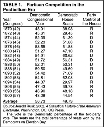
The era from Reconstruction until the realignment of 1896 was characterized by an evenly divided nation and competitive national elections. As Table 1 shows, the nationwide vote for Congress was a virtual tie. Between 1870 and 1900, the Democrats averaged 50.7% of the two-party congressional vote and a similarly razor-thin 49.73% of seats in the House. This close balance between the national parties resulted from the combination of strong Democratic states in the South (on the end of Reconstruction), strong Republican states in the Northeast, and intense competition throughout the Midwest and Border states.

This split within the national electorate was also reflected in the fragile partisan control of national political institutions. Divided government was common during this period (Stewart 1991). But as Stewart and Weingast (1992) demonstrate, the strategic admittance of pro-Republican Western territories into the Union gave the Republicans a structural advantage that allowed them to control both the Senate and presidency for most of this period. Thus, whether partisan control of the national government was unified or divided often pivoted on which party could capture the House of Representatives. Between 1870 and 1900, each party controlled the House in exactly half of the Congresses (eight times apiece). Republicans dominated the House in the years immediately after the Civil War, but their hold on this chamber soon gave way to sharp contestation. The reappearance of Democratic southern delegations beginning in the early 1870s, coupled with the party's success nationally in the 1874 midterm election, created a highly competitive two-party system in the House. With voter loyalties that were tough to change (Silbey 1991) and mobilization efforts near their maximum (Burnham 1982), parties found extra sources of advantage in the clever manipulation of congressional districts.
Compared to their modern counterparts, 19th-century parties in control of state governments were afforded a large degree of discretion in choosing both the timing and the nature of their redistricting events. Part of this redistricting activity was exogenously driven by population increases and a growing number of representatives in the House. Thus, many states were given new seats every 10 years, prompting new district arrangements. But not all of this redistricting activity was prompted by changes in population. Some states chose to redistrict even when they did not gain or lose a seat in the federal apportionment. Moreover, a number of states chose to redistrict more than once a decade.2
When a new party captured unified control of state government and the current districts were written by the newly deposed “out-party,” the likelihood of redistricting substantially increased. Otherwise, the probability of a redistricting event (absent a gain or loss in seats) was almost zero. One reason for the more frequent occurrence of mid-decade redistricting can be found in the prevalence of unified state government. Seventy-nine percent of state elections between 1870 and 1900 resulted in unified government (Burnham 1986). By comparison, between 1970 and 2002, only 49% of state elections ended with unified government (National Council of State Legislatures 2003).
The Ohio state constitution did not give the governor a veto, leaving the legislature relatively unconstrained in drawing congressional districts. At the same time, the state constitution required that a three-person commission (the governor, lieutenant governor, and state auditor) draw up the state legislative districts following narrow guidelines detailing how and when state districts should be redrawn. This prevented parties from gerrymandering the state legislature, helping contribute to that chamber's frequent alternation of party control.
In addition to deciding when to redraw district lines, state legislatures had broad discretion in determining how to draw district maps. Unlike modern state legislatures, they were not bound by the “one-person, one-vote” requirements. Although Congress occasionally added language to the decennial Apportionment Act requiring that districts contain equal numbers of people, there is little evidence that these provisions were ever enforced, much less achieved.
Once a party decided to gerrymander, its members typically pursued one of two strategies. The first was to pack supporters of the opposition into one or a few districts and distribute in-party loyalists evenly throughout the rest of the state in marginal, yet winnable, districts. A good example of this “packing” strategy comes from postreconstruction Alabama, where the majority Democrats placed every possible Black Belt (i.e., Republican) county into one district (the “Old Fourth Alabama”), preferring “to lose one district rather than run the risk of a Republican triumph by a much smaller majority in several districts” (McMillan 1978, 222).
The second strategy was to create an efficient or “dispersal” gerrymander (Cain 1985; Owen and Grofman 1988). A party that was confident in its ability to win the statewide vote for the foreseeable future could maximize its seat share by having each district mirror this favorable statewide partisan distribution (Cain; Cox and Katz 2002). By efficiently distributing its supporters in marginal but winnable districts, the controlling party could win every seat in the state. An illustration of this efficient strategy comes from Maine, where Republicans gerrymandered the state in 1884 and, for the next five elections, captured all four congressional districts despite an average district vote of only 54%.
These anecdotes suggest that state politicians recognized the payoffs in the currency of congressional delegation share from gerrymandering. The possibility that these state-level decisions might also shape the national balance of power was not lost on national party leaders. For example, the Democrats' precarious hold on the U.S. House entering the midterm elections of 1878 led the Speaker of the House, Samuel Randall (D-PA), to implore the Democratic leadership of Ohio to redraw its congressional districts. In April 1878, The New York Times (NYT) gave the following report:
Samuel J. Randall, Speaker of the House of Representatives, has written to leading Ohio Democrats that it is of the utmost importance to the Democratic Party that the Ohio Legislature should redistrict the state. Mr. Randall gives as a reason that the indications point to Republican success in carrying the next House unless some effort of this kind is made by Democrats where they have power (NYT, April 23, 1878, p. 4. col. 6).
STACKING THE STATES: PARTISAN BIAS AND ELECTORAL RESPONSIVENESS
Were state parties using redistricting to stack their state congressional delegations and possibly alter the partisan composition of the House? To answer this question, I begin by analyzing the effect of districting partisanship on the translation of votes into seats. Following standard reasoning in the redistricting literature, one can think of districting plans as affecting two elements of the vote–seat translation—partisan bias and electoral responsiveness (e.g., Gelman and King 1994; Tufte 1973). Partisan bias is defined “as the difference between the expected seat share that the Democrats would get with an average vote share of 0.5 and their “fair share” of 0.5 (half the seats for half the votes)” (Cox and Katz 1999, 820). A districting plan that packs Republican voters into a few safe districts and places Democrats in a number of marginal yet winnable districts would produce a pro-Democratic bias (i.e., they would win more than their “fair-share” of seats given their overall vote).
Responsiveness (or swing ratio) is the change in a party's aggregate seat share given a one-percent change in their vote share. For example, a responsiveness value of three (i.e., the cube law) means that a shift in the statewide vote from 50% to 51% would produce a three-percentage-point seat shift. A districting plan with a number of marginal, highly competitive districts will have a high value of responsiveness (i.e., a small swing in the statewide vote will generate a large swing in seats). A plan with numerous safe seats will have a lower level of responsiveness because it will take a large swing in the statewide vote before seats start changing hands.
If parties used redistricting to tilt electoral outcomes in their favor, then plans passed when a single-party-controlled state government should lead to high levels of both responsiveness and partisan bias. A bias in favor of the controlling party is consistent with that party skewing the districts in their favor. Although plans passed during divided state governments were rare in the 19th century, there were a few, and their dynamics differed from partisan plans. Because both parties could veto the other's schemes, bipartisan plans typically protected incumbents of both parties. We should, therefore, expect to see lower levels of bias and responsiveness under bipartisan plans (Cox and Katz 2002).
To estimate bias and responsiveness for redistricting plans passed between 1870 and 1900 I matched the precise date of each redistricting (Martis 1982) with the partisan composition of the state legislatures and governors at the time of passage (Burnham 1986). With this information, I then assigned each election, by state and year, to one of three plans: partisan Democratic, partisan Republican, and bipartisan (taking into account the various veto override provisions; Cox and Katz 2002).
Following standard practice in the electoral systems literature (e.g., Grofman 1983; Tufte 1973), I estimated the following vote–seat equation,

where sit is the proportion of seats won by the Democrats, and vit is their vote share in state i at time t.4
Beginning with the Apportionment Act of 1872, Congress allowed states to elect any newly gained seats in at-large elections if for some reason they failed to redistrict. In calculating the proportion of Democratic seats, I excluded at-large seats. Including them does not change the results.
Bias is typically calibrated to what would have happened if the vote were split 50–50. Thus the bias estimates reported in Table 2 are the result of passing λ through the following equation: exp[λ]/(exp[λ]+1) −0.5.
In this analysis, I use the statewide total Democratic vote. Using the total vote, as opposed to the average across districts, captures biases arising from both the distribution of voters and from malapportionment (Grofman, Koetzle, and Brunell 1997).
States with only one seat or states that elect their entire delegation at-large are excluded.
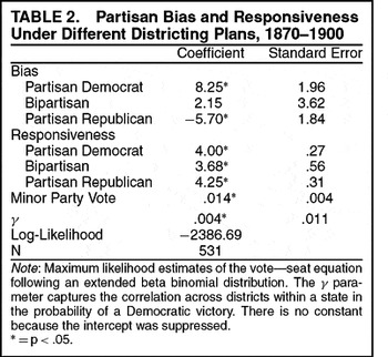
The estimates in Table 2 show that the partisanship of districting plans directly affected the translation of votes into seats. Partisan Democratic plans produced a significant bias of 8.3% (in other words, for 50% of the vote, Democrats received 58.3% of the seats). Partisan Republican plans produced a significant bias of 5.7% in favor of the GOP. Bipartisan plans, however, failed to produce significant levels of bias. Substantively, these results indicate that the partisanship of districting plans was systematically related to outcomes on Election Day. At 50% of the vote, a party could expect to win roughly between 58% and 44% of a state delegation depending on which party drew the district lines.

Both types of partisan plans produced high levels of responsiveness—4.0 and 4.25 for Democratic and Republican plans, respectively. Bipartisan plans, as expected, produced a lower level of responsiveness (3.68) than the two partisan plans. These levels are substantially higher than any found in the 20th century (Brady and Grofman 1991; Engstrom and Kernell 2005).8
The estimates in Brady and Grofman (1991) show an average swing ratio of 3.98 in the 19th century (1850 to 1900) and 2.13 in the 20th century (1900–80). Engstrom and Kernell (2005, 542) estimate an average swing ratio of 4.64 between 1840 and the 1890s (in non-Southern states). This dropped to 3.48 after widespread adoption of the Australian ballot (the analysis stops at 1940).
Efficient gerrymanders were, in part, made possible because incumbents were not in a strong position to push for safer districts. Though this was a period of emerging careerism (Price 1975), congressmen were still at the mercy of local political organizations for nomination and access to the ballot. Moreover, the importance of seniority in determining committee positions had yet to fully take root (Katz and Sala 1996).
An intriguing implication is that the frequency and partisanship of redistricting may have contributed to this era's high retirement rates and helped slow the development of congressional careerism. If parties were more willing to pursue extra seats rather than protect sitting representatives, we should find incumbents more readily retiring when their district was altered. In comparing incumbent retirement rates in redrawn and untouched districts this is precisely what we find. Between 1870 and 1900 only 54% of incumbents who had their district redrawn ran for reelection. By comparison, in untouched districts 69% of incumbents sought reelection (the difference is significant at .01).
THE PARTISAN CONSEQUENCES OF REDISTRICTING
The results in the previous section are consistent with the hypothesis that parties drew electoral maps to bias outcomes in their favor. Here we consider the intent behind redistricting plans. In the 19th century, strategic state legislators took the most recent election results, broken down by county and ward, and combined these data to forecast the partisan effects of new district lines. Because counties were the building blocks of most districts, politicians could easily aggregate county vote returns and calculate the partisan consequences of new district lines. For example, the Republican governor of Ohio, Joseph Foraker, bragged to the New York Times that the Republican gerrymander in 1886 would allow his party to capture 14 of Ohio's 21 Congressional seats (NYT, May 18, 1886, p. 1, col. 4). Foraker's dead-on predictions were based on the aggregation of the 1884 presidential vote by county into the newly drawn district lines. These simple forecasting exercises, therefore, appeared to be standard practice for those redrawing district lines. With the use of historical election results and 19th-century congressional district maps, I can do the same.
To do this, I took the two-party congressional vote by county (Clubb, Flanigan, and Zingale 1987) from the most recent election before a new redistricting and then aggregated the county results into the new district lines (Martis 1982). When district lines crossed county boundaries or multiple districts were contained within a single county (e.g., New York, Philadelphia, and Chicago), I tracked down the necessary ward- and town-level election data.9
In almost all of these cases, I used either state-legislative election returns or the presidential votes reported at the ward and town level. These sources are available on request. In some instances, I was also able to use contemporary reports from the New York Times for corroboration. The only case I was forced to exclude was the Massachusetts redistricting of 1892 because the district lines cut across too many county boundaries.
To measure the effect of partisanship on the intent of district plans, I estimated an equation where the dependent variable is the intended change in the Democratic proportion of seats (i.e., the postredistricting proportion minus the pre-redistricting proportion). The key independent variable is the partisanship of those responsible for drawing the new districts (Born 1985). This latter variable, Partisanship, is coded +1 for Democratic plans, 0 for bipartisan plans, and −1 for Republican plans. If parties reconstruct district lines to add to their congressional delegation, then this variable should be positive and significant. In addition, I also included the proportion of congressional seats Democrats held at the time of redistricting (Lag Seat%) because it is harder for a party to add seats if they already hold most, or all, of the congressional delegation (see Born). A variable indicating whether a state lost or gained seats in the federal apportionment is also included as a control. This variable is scored 1 for a gain, zero for no gain, and −1 if a state lost seats. Finally, the analysis is confined to states with more than two congressional seats.
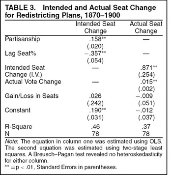
The results are presented in the first column of Table 3. The coefficient for Partisanship is indeed positive and significant (p<.01). The value of the coefficient is .158, indicating that going from a bipartisan plan to a Democratic plan increased the intended Democratic gain to 15.8% of the delegation, and going from a Republican to a Democratic plan meant a substantial switch of 31.6% of the delegation. In a state with twenty congressional seats (such as Ohio for much of this period) we would expect that going from a Republican to a Democratic redistricting plan would produce, on average, an intended swing of roughly six seats to the Democrats.

Of course, intent may not match reality on Election Day. The best laid plans of strategic mapmakers may be undone by shifting partisan tides, changing migration patterns, or merely poor calculations. To investigate the correspondence between intent and the results, I borrowed the technique used by Born (1985) in his study of modern redistricting. This technique regresses the actual change in the Democratic delegation (Actual Seat Change) on the intended seat change. In addition, the change in the Democratic vote share (Actual Vote Change) and whether a state lost or gained seats are included as controls. Because the actual shift in seats is endogenous with the intended change, a standard OLS equation would be inappropriate. Instead, two-stage least squares is employed. In the first stage, Intended Seat Change is regressed on the independent variables Partisanship, Gain/Loss in Seats, Lag Seat%, and Actual Vote Change. The predicted values for Intended Seat Change from this first stage can then be used as an instrumental variable that is plugged into the second stage equation. The coefficient of this instrumental variable will indicate to what extent the intentions of partisan mapmakers came to fruition.
The results are presented in the second column of Table 3. The positive (.871) and significant coefficient for intended vote change suggests a close correspondence between intent and Election Day outcomes.10
As a comparison, Born (1985; 312–13) estimates a coefficient of .771 for the period 1952 to 1982, and .668 when he restricts the sample to the period after the reapportionment revolution (1966–82).
Models including state and year-fixed effects produced largely similar results. Using the presidential vote, instead of the congressional vote, predicted the intended change slightly worse and the actual outcomes slightly better than the congressional vote, but also contained an occasional large miss (i.e., when the most recent presidential election was 4 years prior to the redistricting). I preferred to use the most recent electoral results possible because the politicians drawing the maps likely used them.
As the overall pattern of results indicates, 19th-century politicians were clearly adept at achieving the two necessary conditions for a successful partisan gerrymander: they systematically drew state electoral maps to bias elections in their favor, and these efforts were largely realized at election time. In the next section, I examine the degree to which these state-level decisions cumulated to influence party ratios in the House of Representatives and the overall national balance of power.
STACKING THE HOUSE
Since most of what was intended in redistricting plans came to fruition, one can take the state-by-state intended effects of redistricting for each year and simply add them together to see how many national seats can be attributed to gerrymandering. So, for each year, I took the number of seats each party gained via gerrymandering and summed them to get a net redistricting effect. These numbers can then be used to develop counterfactuals for party ratios in the House. In other words, one can compare the effects of gerrymandering with what would have happened in the absence of gerrymandering.
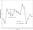
The results of this simulation are presented in Figure 2. The figure compares the simulation to the actual party ratios in the House. There are a number of instances in which the simulation differs from actual history. In 1882, for example, gerrymandering padded the Democratic majority by 14 seats. In 1890, Democratic efforts in Ohio wrested seven seats away from the Republicans. In a couple of instances, pro-Democratic gerrymanders were counteracted by pro-Republican gerrymanders. For example, in 1880, Democrats picked up two seats from gerrymandering; and Republicans, four, for a net of only two seats.

Counterfactual Composition of the U.S. House, 1870–1900
Perhaps more important are the elections of 1878 and 1888 in which gerrymandering actually helped determine party control of the House. In 1878, the nine seats Democrats picked up via Ohio's and Missouri's gerrymandering allowed Democrats to retain majority control. Without these nine seats, the Democrats would not have had a majority in the House. In addition, the Democratic capture of the House prevented the Republicans from gaining unified control of the national government. In 1888, Republicans in Pennsylvania carved 21 pro-Republican districts out of 28 total despite only having 53% of the statewide two-party vote. This was just enough to put the Republicans over the top in the U.S. House, and it also gave them unified party control of the national government. This was also the Congress in which the Republican Speaker—Thomas Brackett Reed—crafted “Reeds” rules, subsequently reshaping legislative procedure within the House (Binder 1997; Schickler 2001).
There were also some near-misses. For instance, in 1876, Democratic gerrymanders in three Southern states (Alabama, Arkansas, and Mississippi) helped solidify an otherwise tenuous Democratic majority in the House. Given Republican control of the Senate and the presidency, these gerrymanders helped provide the Democrats with an institutional bulwark to fight the Republican Reconstruction agenda.
CONCLUSION
Strategic politicians in America have always behaved as if redistricting offers a golden opportunity for partisan advantage. The image of politicians manipulating district lines for partisan gain suggests that the path to national power may run through the state legislatures (Born 1985). Yet, political science research on congressional redistricting in the 1970s, 1980s and 1990s has found, at most, only minimal national partisan consequences (e.g., Campagna and Grofman 1990; Swain, Borrelli, and Reed 1998). In this article, I have addressed this debate by taking a historical step back and examining the partisan consequences of redistricting in the late 19th century. My general finding is that between 1870 and 1900 redistricting systematically influenced state party delegations in ways that occasionally cumulated into substantial national effects.
First, I found that the partisanship of districting plans systematically affected the translation of congressional votes into legislative seats. Parties in control of the districting process were able to engineer favorable vote–seat translations, which allowed them to magnify their share of state congressional delegations. The difference between Republican- or Democratic-drawn district lines meant a difference of roughly 14% of the congressional delegation. Second, by closely examining county-, ward-, and town-level vote returns before and after redistricting, I found further evidence of the successful use of gerrymandering for partisan advantage. Third, these state-level effects, at times, produced important national-level consequences. On at least two occasions, it appears that gerrymandering helped determine party control of the House.
These results also have important implications for our understanding of the institutional development of Congress. In the conventional portrait of the 19th-century House, seats frequently turn over, little value is placed on seniority, and the tenures of MC's are brief (e.g., Katz and Sala 1996; Kernell 1977). One explanation for the tumult within the 19th-century House is the instability of many congressional districts. Elections to the House in the 19th century were noted for their competitiveness and turbulence (e.g., Brady 1988; Carson and Roberts 2005). Small shifts in the vote could easily end the career of an individual MC, produce large swings in the aggregate seat share, and even, at times, change party control of the House. Here I have identified redistricting as an important, but often overlooked, component of the explanation for the turbulence of 19th-century House elections.
The reversals in party fortunes within the House also carried with it direct implications for national policymaking. During this period, the House was often the pivotal branch that determined whether control of the federal government was unified or divided. Given the deep partisan polarization over issues such as federal policy in the South (Kousser 1992) and the tariff (Stewart 1991), control of the House was a key ingredient for parties seeking to shape the direction of federal policy. As such, gerrymandering served as a potent tool in the pursuit of state and national power.
From this perspective, it is not surprising that strategic politicians have again turned to partisan gerrymandering in the bid for national power. The relatively tight national balance between the two parties in the current period has once again raised the payoffs from the manipulation of electoral institutions. The similarities between 19th-century American politics and recent mid-decade redistricting events in Texas and Georgia indicate that congressional redistricting is not exempt from partisan politicians' efforts to stack the electoral deck in their favor.
An earlier version of this paper was presented at the 2003 Meeting of the American Political Science Association and the 2003 Meeting of the Midwestern Political Science Association. Thanks to Sam Kernell, Gary Cox, Daniel Lipinski, Nathan Monroe, Michael Crespin, Randall Strahan, Georg Vanberg, the anonymous reviewers, and seminar participants at George Washington University for helpful comments.



Comments
No Comments have been published for this article.