1. The Optimality of Meta-induction: A Solution to the Problem of Induction?

Schurz (Reference Schurz2008) developed a new account to the problem of induction that is based on the optimality of meta-induction. The account agrees with Hume’s skeptical insight that it is impossible to demonstrate a priori that induction is reliable in the sense that it is predictively more successful than random guessing. Such a demonstration is impossible without assuming that the actual world possesses a certain amount of regularity. Reichenbach (Reference Reichenbach1949, sec. 91) argued that it is at least possible to demonstrate a priori that induction is optimal, that is, is the best what we can do for the purpose of predictive success. Results in formal learning show, however, that it is not possible to demonstrate optimality at the level of object-induction, that is, of induction applied to the task of predicting events in arbitrary possible worlds (cf. Skyrms Reference Skyrms2000, sec. III.4). In contrast, what the account of meta-induction attempts to show is that induction is optimal if it is applied at the meta-level of competing prediction methods. The meta-inductive strategy tracks the success rate of all prediction methods whose predictions are accessible and predicts an optimal weighted average of the predictions of those methods that were most successful so far. Using results in the theory of regret-based online learning (Cesa-Bianchi and Lugosi 2006), Schurz (Reference Schurz2008) proved that there exists a particular weighting method, called attractivity-weighting, which grants the meta-inductivist a predictive success rate that is in the long run at least as high as that of every other prediction method that is accessible to the meta-inductivist. Since the restriction to accessible methods is crucial for the optimality theorem, Schurz and Thorn (Reference Schurz and Thorn2016) call this kind of optimality access-optimality. Remarkably, the access-optimality of meta-induction holds in all possible worlds, even in ‘chaotic’ worlds in which the event frequencies and success rates do not converge against limits but are permanently changing in irregular ways, or in ‘paranormal’ worlds that host perfect clairvoyants or demonic deceivers.

Technically the account of meta-induction is based on the notion of a prediction game:

The predictive success rate of a method P is defined by means of the following chain of definitions:

• • pred_n(P) is the prediction of player P for time n delivered at time $n-1$,

• • the deviation of the prediction pred_n from the event e_n is measured by a normalized loss function, $\mathrm{loss}\left({\mathrm{pred}}_n,e_n\right)\in \left[0,1\right]$,

• • $\mathrm{score}\left({\mathrm{pred}}_n,e_n\right){=}_{\mathrm{def}}1-\mathrm{loss}\left({\mathrm{pred}}_n,e_n\right)$ is the score obtained by prediction pred_n of event e_n,

• • ${\mathrm{abs}}_n\left(P\right){=}_{\mathrm{def}}{\sum }_{1\le i\le n}\mathrm{score}\left({\mathrm{pred}}_i\left(P\right),e_i\right)$ is the absolute success achieved by player P until time n, and

• • ${\mathrm{suc}}_n\left(P\right){=}_{\mathrm{def}}{\mathrm{abs}}_n\left(P\right)/n$ is the success rate of player P at time n.

The natural loss function is defined as $\left|{\mathrm{pred}}_n-e_n\right|$. The optimality theorem below holds for all convex loss functions, which means that the loss of a weighted average of two predictions is not greater than the weighted average of the losses of two predictions. In what follows we assume convex loss functions; they comprise a large variety of loss functions including all linear, polynomial, or exponential functions of the natural loss function.

‘Possible worlds’ are identified with prediction games. A special case are binary games whose events and predictions are elements of {0,1}. For binary games the natural loss function coincides with the zero-one loss: ${\mathrm{loss}}_{1-0}\left(\mathrm{pred},e\right)=0$ if $\mathrm{pred}=e$, and $\mathrm{otherwise}=1$.

The simplest meta-inductive strategy is called “imitate-the-best” and predicts what the currently best non-MI player predicts. It is easy to see that this meta-inductive method cannot be universally access-optimal: its success rate breaks down when it plays against non-MI methods that are deceivers, which means that they lower their success rate as soon as their predictions are imitated by the meta-inductivist (cf. Schurz Reference Schurz2008, sec. 4). A realistic example is the prediction of stock values in a ‘bubble economy’: here the prediction that a given stock will yield a high rate of return leads many investors to put their money on this stock, and by doing so they cause it to crash. Nevertheless there exists a meta-inductive strategy that is provably universally optimal. This strategy is called attractivity-weighted meta-induction (wMI) and is defined as follows:

Definition 2. The predictions of wMI (attractivity-weighted meta-induction) are defined as

${\mathrm{pred}}_{n+1}\left(\mathrm{wMI}\right){=}_{\mathrm{def}}\frac{{\sum }_{1\le i\le m}{\mathrm{at}}_n\left(P_i\right)\times {\mathrm{pred}}_{n+1}\left(P_i\right)}{{\sum }_{1\le i\le m}{\mathrm{at}}_n\left(P_i\right)},$

where

• • at_n(P_i) is the attractivity of a player P_i for wMI at a given time n, defined as ${\mathrm{at}}_n\left(P_i\right){=}_{\mathrm{def}}{\mathrm{suc}}_n\left(P_i\right)-{\mathrm{suc}}_n\left(\mathrm{wMI}\right)$, if this expression is positive; else ${\mathrm{at}}_n\left(P_i\right)=0$, and

• • if $n=1$ or the denominator is 0, wMI’s prediction is a random guess.

Attractivity at_n(P_i) is also called wMI’s regret compared to P_i (at time n), and attractivity-weighted meta-induction is a case of regret-based learning. Let “maxsuc_n” denote the non-MI-players’ maximal success rate at time n. Then the optimality theorem for wMI asserts (see Schurz Reference Schurz2008, sec. 7, theorem 4):

According to theorem 1.2 attractivity-weighted meta-induction is long-run optimal for all possible event sequences and sets of accessible prediction methods. The only proviso is that the set of accessible methods is finite, which is a realistic assumption for cognitively finite beings. In the short run, weighted meta-induction may suffer from a possible loss, compared to the leading player. This loss is caused by the fact that wMI must base her prediction of the next event on the past success rates of the candidate methods, and the hitherto most attractive methods may perform badly in the prediction of the next event. Fortunately theorem 1.1 states a worst case upper bound for this loss, $\sqrt{m/n}$, which is small if the number of competing methods, m, is small compared to the number of rounds, n, and which converges quickly to zero when n grows large.Footnote ¹

Theorem 1 applies to prediction games with real-valued as well as binary (or discrete) events. Even if the events are binary wMI’s predictions are real valued (because proper weighted averages of zeroes and ones are real valued). How can the optimality result of theorem 1 be transferred to binary games whose predictions must be binary? There are two methods by which this can be done:

1. 1. Randomization, rwMI (Cesa-Bianchi and Lugosi Reference Cesa-Bianchi and Lugosi2006, sec. 4.1): Here one assumes that rwMI predicts $e_n=1$ with a probability (P) that equals the optimal real-valued prediction of wMI; that is, $P\left({\mathrm{pred}}_n\left(\mathrm{rwMI}\right)=1\right)={\mathrm{pred}}_n\left(\mathrm{wMI}\right)$. This method is not entirely general since it presupposes that the events are probabilistically independent from rwMI’s choice of prediction.

2. 2. Collective meta-induction, cwMI (Schurz Reference Schurz2008, sec. 8): Here a collective of meta-inductivists approximates real-valued predictions by the mean value of their binary predictions. Their mean predictive success rate approximates provably the success rate of the optimal method wMI. Assuming that the cwMIs are cooperators and share their success, every individual member of the collective is predictively optimal.

Theorem 1 establishes the following a priori justification of attractivity-weighted meta-induction: in all environments it is reasonable—in addition to searching for good object-level methods—to apply the strategy wMI, as this can only improve but not worsen one’s success in the long run. Note that by itself this justification does not entail anything about the rationality of object-level induction: it may well be that we live in a world in which a method different from object-induction is predictively superior. However, the a priori justification of meta-induction gives us the following a posteriori justification of object-induction: to the extent that so far object-inductive prediction methods were more successful than all accessible noninductive (object-level) prediction methods, it is meta-inductively justified to continue favoring object-inductive prediction methods in the future.

Theorem 1 asserts the optimality but not the dominance (in the long run) of attractivity-based meta-induction. Thus, there may exists other methods, different from wMI, that are likewise long-run optimal. In fact one can prove that there are certain variants of wMI that are long-run optimal and have short-run advantages in certain environments and disadvantages in others. So wMI cannot be universally long-run dominant. Nevertheless, the following restricted dominance result for wMI follows from theorem 1:

Theorem 2 is crucial for the next sections in which we confront the optimality of meta-induction with the no free lunch theorem.

2. Radical Inductive Skepticism: The No Free Lunch Theorem

The (in)famous no free lunch (NFL) theorem is a radicalized version of Hume’s inductive skepticism for theoretical computer science.Footnote ² The theorem applies to prediction methods that can be represented as computable functions from past observations to predictions, so-called learning algorithms (thus, clairvoyance is excluded). The theorem is often expressed by the assertion that for each pair of prediction methods, the number—or in the infinite case, the probability—of possible worlds (event sequences) in which the first method outperforms the second is precisely equal to the number (or probability) of worlds in which the second method outperforms the first. We call this assertion the strong NFL theorem, because it presupposes a ‘homogeneous’ loss function:

The requirement of a homogeneous loss function is very strong: it is only satisfied if events and predictions are binary or, more generally, if they both discrete with $\mathrm{Val}={\mathrm{Val}}_{\mathrm{pred}}$ and a zero-one loss function. Under this assumption homogeneity is obvious: if the value space has k elements, then for every $\mathrm{pred}\in \mathrm{Val}$ the number of possible events $e\in \mathrm{Val}$ that lead to a loss of 1 is obviously $k-1$, and the number of events that lead to a loss of 0 is one. In contrast, in prediction games with real-valued predictions the homogeneity requirement fails. In the binary case, for example, the number of events that lead to a loss of 1 is one for the two predictions $\mathrm{pred}=1$ and $\mathrm{pred}=0$ but zero for the prediction $\mathrm{pred}=0.5$.

Homogeneous loss functions are a clear restriction of the strong NFL theorem. Real-valued predictions make sense not only for real-valued but also for binary events (e.g., by predicting their probabilities). Moreover (as explained) they can be implemented in binary games by randomization over binary predictions or by a cooperative collective of binary forecasters. There is, however, a weak version of the NFL theorem (mentioned by Wolpert Reference Wolpert1996, 1354) that applies to real-valued predictions over binary or discrete events and assumes what we call a “weakly homogeneous” loss function:

For binary events with real-valued predictions and a natural loss function, weak homogeneity is satisfied since for every prediction $\mathrm{pred}\in \left[0,1\right]$, $\mathrm{loss}\left(\mathrm{pred},1\right)+\mathrm{loss}\left(\mathrm{pred},0\right)=1-\mathrm{pred}+\mathrm{pred}=1$.

For prediction games with real-valued events, most loss functions (including all convex ones) are not even weakly homogeneous. Here “free lunches” are possible in the sense that not all prediction methods have the same expected success, relative to a state-uniform probability distribution.

In this article we focus on prediction games with discrete events and real-valued predictions, to which the weak NFL theorem applies. Wolpert (Reference Wolpert1996) proves the NFL theorems in the framework of learning algorithms that map training sets into predictions of test items. A prediction game can be considered as an iteration of the procedure of selecting the first n events as a training set and the next event as a test item, that is, the test item of the nth round is added to the training set of the next round. Because a state-uniform prior induces a state-uniform conditional distribution $P\left(e_{n+1}|\left(e_1,\dots ,e_n\right)\right)$, the NFL theorem applies straightforwardly to the (expected) scores in each round of a prediction game and thus (by the linearity of expectation values) to the (expected) score sums in the entire game.Footnote ³

Theorem 4 implies that every possible prediction method—be it an intelligent inductive one, a crazy anti-inductive one, or a stupid one that always predicts the same value—has the same expected predictive success relative to a state-uniform prior distribution. For all induction-friendly philosophical programs, including the program of meta-induction, this result seems to be devastating. How is it possible? In what follows we give a brief explanation of theorem 4 in terms that are philosophically more familiar than Wolpert’s “extended Bayesian framework.”

Wolpert’s NFL theorem is a far-reaching generalization of a straightforward result about the prediction of binary sequences. For this application the NFL theorem rests on the following fact: however a prediction function f, with ${\mathrm{pred}}_{n+1}=f\left(\left(e_1,\dots ,e_n\right)\right)\in \left\{0,1\right\}$, is defined, there are as many sequences of a given length $k>n$ extending (e₁, …, e_n) that verify f’s prediction ${\mathrm{pred}}_{n+1}$ as there are sequences that falsify it. Thus, by attaching an equal probability to every possible sequence, the expected score of each prediction function will be $1/2$. The same observation is the content of an (in)famous result in probability theory that can be found (among other works) in Carnap (Reference Carnap1950, 564–66) or Howson and Urbach (Reference Howson and Urbach1996, 64–66). The result can be expressed as follows:

3. No Free Lunch and Meta-induction—a Conflict?

We now turn to the relation between the weak NFL theorem and theorem 2 about meta-induction. The NFL theorem applies not only to object-level prediction methods but also to all meta-strategies, given that they are applied to a fixed set of independent prediction methods—for the reason that every combination of a finite number of prediction algorithms is itself a prediction algorithm. So the puzzling question arises: If the NFL theorem is true, how can it be that attractivity-weighted meta-induction, when applied to a fixed set of independent prediction algorithms, is dominant in comparison to certain other methods, as stated in theorem 2? Is this a contradiction?

Our answer to this question in regard to the long-run perspective can be summarized as follows: no, the contradiction is only apparent. It is indeed true that there exist many wMI-accessible methods whose predictive success rate is (in the long run) strictly smaller than that of wMI in some worlds (event sequences) and never greater than that of wMI in any world—let us call these methods M_inf (for “inferior”).Footnote ⁵ Nevertheless, the state-uniform expectation values of the success rates of wMI and M_inf are equal because a state-uniform distribution assigns a probability of 0 to all worlds in which wMI dominates M_inf, so these worlds do not affect the probabilistic expectation value. Put into a nutshell, for weakly homogeneous loss functions free lunches exist but receive a probability of 0 under a state-uniform prior.

Let us elaborate on this connection. The major difference between the account of meta-induction and Wolpert’s extended Bayesian account is this: while the former account is independent from any assumed prior distribution over possible event sequences, Wolpert’s result depends on a particular prior distribution, the state-uniform distribution. Wolpert seems to assume that this distribution is epistemically privileged. Reasonable doubts can be raised here because the state-uniform distribution is induction hostile. A proponent of this distribution is a priori certain that the binary event sequence she is going to predict (a) has a limiting frequency of $1/2$ and (b) is noncomputable. Fact a follows from theorem 5, and b from the fact that there are uncountably many sequences but only countably many computable ones. However, the event sequences for which an intelligent prediction method can be better than random guessing or any other ‘stupid’ method are precisely those event sequences that do not fall into the intersection of classes a or b. Let us make this point explicit: for random sequences with a limiting frequency of $1/2$, all combinations of independent methods must have the same success rate as random guessing (i.e., $1/2$). The only possibility for these sequences to be predictable is that they are computable by an internal regularity, but this possibility has probability 0, too.

In conclusion, proponents of a state-uniform prior distribution are strongly biased: they are a priori certain that the world is irregular so that induction cannot have any chance. We suppose that adherents of a more induction-friendly view, for example, Bayesians in the ordinary (not Wolpertian) sense, will regard a state-uniform prior distribution as highly “unnatural.” Instead of a state-uniform distribution, they typically prefer a uniform distribution over all possible limiting frequencies; we call such a distribution a frequency-uniform distribution. It is well known that frequency-uniform distributions are highly induction friendly: from them one can derive Laplace’s rule of induction,

$P\left(e_{n+1}=1|f_n\left(1\right)=\frac{k}{n}\right)=\frac{k+1}{n+2},$

where “f_n(1)” denotes the frequency of ones among the first n events (cf. Carnap Reference Carnap1950, 568). In computer science, Laplace’s rule has been generalized by Solomonoff (Reference Solomonoff1964, sec. 4.1), who proved that if the prior probability of a sequence is inversely proportional to its algorithmic complexity, then Laplace’s rule of induction is valid.

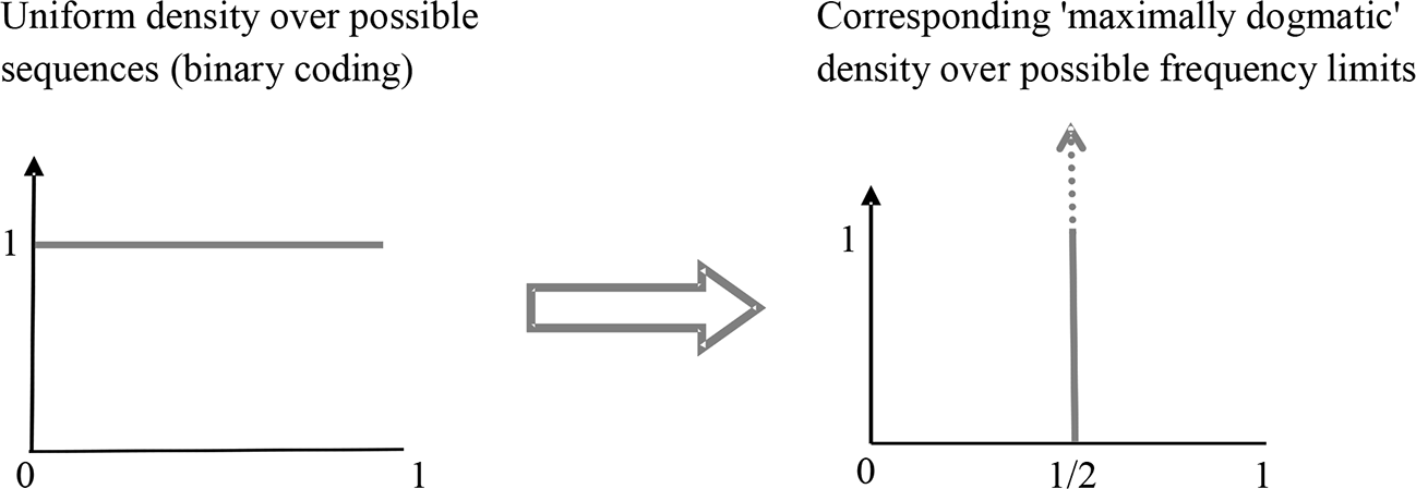
The precise relation between prior distributions over the space of possible infinite sequences and corresponding distributions over the space of possible limiting frequencies (or classes of sequences with the same frequency) is displayed in figures 1 and 2. As usual, infinite 0–1 sequences are represented as real numbers between 0 and 1 in binary representation (e.g., 0.0110…) and ordered according to their numerical size. In this way, the state-uniform distribution over possible sequences is represented as a uniform density over the interval [0,1]. Figure 1 presents the transformation of this distribution into the corresponding distribution over possible limiting frequencies, with the result that a uniform distribution over [0,1] viewed as space of sequences is transformed into a maximally dogmatic distribution (an infinite density peak) over [0,1] viewed as space of frequency limits.

Figure 1.

Transformation of a state-uniform distribution into the corresponding distribution over frequencies.

Figure 2.

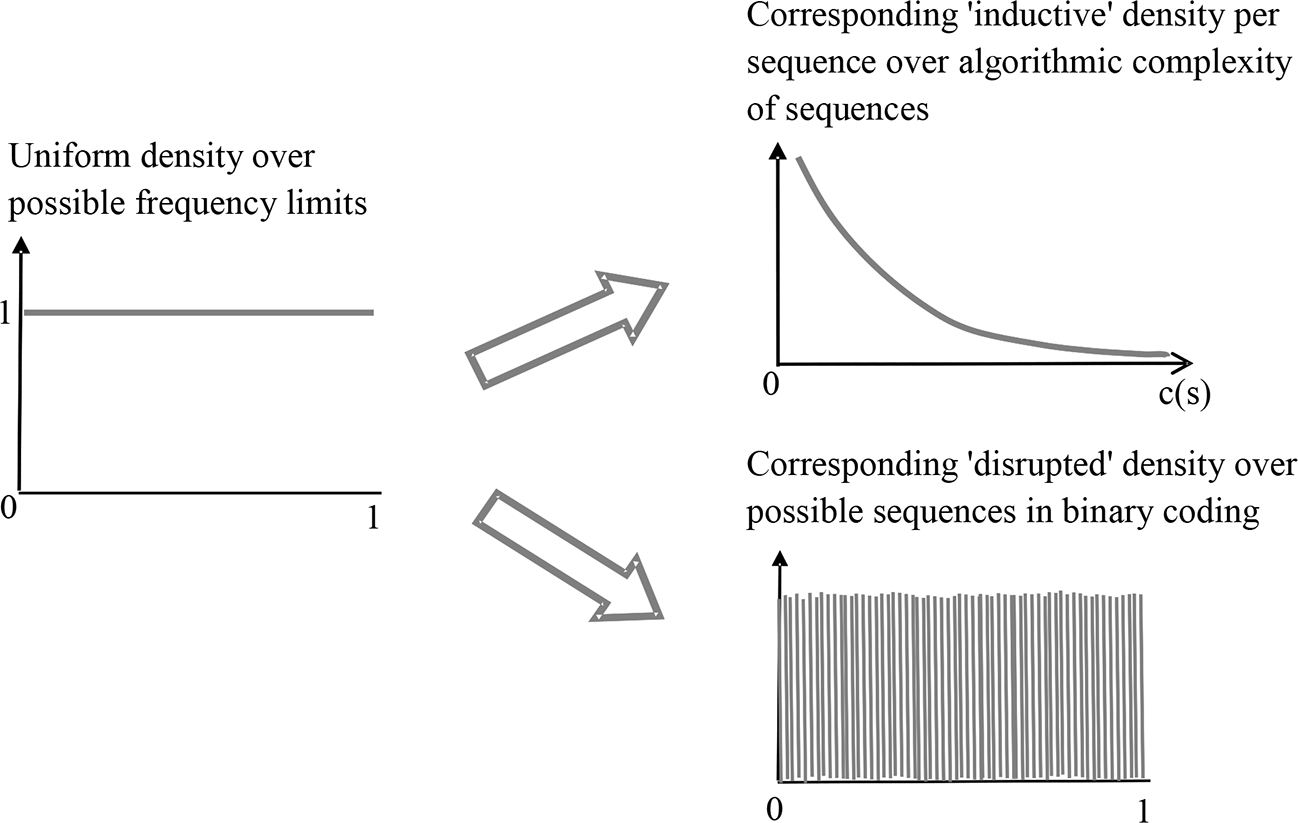
Transformation of a frequency-uniform distribution into the corresponding distribution over the algorithmic complexity of sequences (top) and over sequences in binary coding (bottom).

Figure 2 illustrates the inverse transformation. The upper part of figure 2 displays Solomonoff’s (Reference Solomonoff1964) result, which states that the frequency-uniform probability of a (finite or infinite) sequence decreases exponentially with its algorithmic complexity c(s): $P\left(s\right)~2^{-c\left(s\right)}$. Thus, sequences with lower complexity have a higher frequency-uniform probability than those with high complexity. In conclusion, a frequency-uniform distribution is strongly biased in regard to less complex (more regular) sequences. The lower part of figure 2 shows what happens to a frequency-uniform distribution over [0,1] when it is transformed into a distribution over [0,1] viewed as space of possible sequences. The resulting distribution becomes noncontinuous and disrupted: in every finite interval $I\subseteq \left[0,1\right]$ it increases infinitely often to a maximal value and falls back to a minimal value.Footnote ⁶ It follows that a state-uniform prior distribution makes Bayesian convergence results impossible because all these results presuppose a (not necessarily uniform but) continuous prior distribution over the possible frequencies (Earman Reference Earman1992, 141ff.). Thus, “outwashing of priors” is impossible for state-uniform prior distributions.

So which prior distributions are more natural, state-uniform ones or frequency-uniform ones? In our eyes, this question has no reasonable answer because all prior distributions are subjective and biased in some respect. We regard it as a great advantage of the optimality of meta-induction that it holds regardless of any assumed prior probability distribution. For a frequency-uniform prior distribution the probability of worlds in which meta-induction dominates random guessing is close to 1. For a state-uniform prior the probability of worlds in which meta-induction dominates random guessing is 0. Nevertheless, infinitely many such worlds exist, and it is precisely in these worlds that intelligent prediction methods can have a chance at all. We should certainly not exclude these induction-friendly worlds from the start by assigning a probability of 0 to them. This concludes our discussion of the relation between meta-induction and the NFL theorem within the perspective of the long run.

4. No Free Lunch and Meta-induction in the Short-Run Perspective

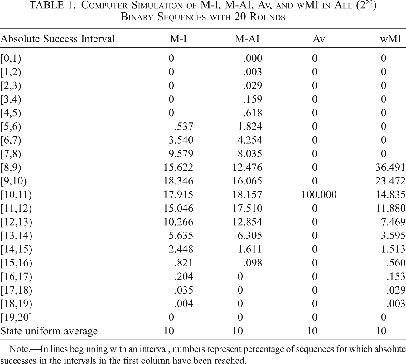
The discussion of Wolpert’s theorem within the perspective of the short run is more intricate. Recall that for finite sequences the advantage of meta-induction comes at a certain cost, which vanishes in the long run but is nonnegligible for short sequences. Table 1 presents the result of a computer simulation of all possible prediction games with a length of 20 rounds, with binary events, three independent prediction methods, and wMI.Footnote ⁷ The considered independent methods were

• • majority induction, M-I, which always predicts the event that so far has been in the majority and is 0.5 in the case of ties (i.e., ${\mathrm{pred}}_{n+1}=1/0.5/0$ if and only if $f_n\left(1\right)>/=/<0.5$, respectively),

• • majority anti-induction, M-AI, which predicts the opposite of M-I (i.e., ${\mathrm{pred}}_{n+1}=0/0.5/1$ if and only if $f_n\left(1\right)>/=/<0.5$, respectively),

• • averaging, Av, which always predicts 0.5.

Table 1 displays the frequencies of sequences for which the absolute success of a prediction method lies in a certain interval, with [0,1) being the lowest and [19,20] the highest possible success interval. In accordance with the weak NFL theorem, one sees that the average success is the same for all four methods. Nevertheless, the frequency distributions over classes of sequences in which these methods reach certain success levels is remarkably different. The averaging method predicts 0.5 always and earns a sum of scores of 10 in all possible sequences. The object-inductive method M-I reaches a high success level in more worlds than the anti-inductive method M-AI (symmetrically, M-AI attains a low success level in more worlds than M-I). In compensation, the number of worlds in which the anti-inductive method does just a little better than averaging is significantly higher than the corresponding number of worlds for the inductive method.

Table 1.

Computer Simulation of M-I, M-AI, Av, and wMI in All (2²⁰) Binary Sequences with 20 Rounds

Absolute Success Interval	M-I	M-AI	Av	wMI
[0,1)	0	.000	0	0
[1,2)	0	.003	0	0
[2,3)	0	.029	0	0
[3,4)	0	.159	0	0
[4,5)	0	.618	0	0
[5,6)	.537	1.824	0	0
[6,7)	3.540	4.254	0	0
[7,8)	9.579	8.035	0	0
[8,9)	15.622	12.476	0	36.491
[9,10)	18.346	16.065	0	23.472
[10,11)	17.915	18.157	100.000	14.835
[11,12)	15.046	17.510	0	11.880
[12,13)	10.266	12.854	0	7.469
[13,14)	5.635	6.305	0	3.595
[14,15)	2.448	1.611	0	1.513
[15,16)	.821	.098	0	.560
[16,17)	.204	0	0	.153
[17,18)	.035	0	0	.029
[18,19)	.004	0	0	.003
[19,20]	0	0	0	0
State uniform average	10	10	10	10

Note. In lines beginning with an interval, numbers represent percentage of sequences for which absolute successes in the intervals in the first column have been reached.

On the basis of these results, we obtain a justification of object-induction and of meta-induction even within the induction-hostile perspective of a state-uniform prior distribution for short-run sequences. One can reasonably argue that what counts is to reach high success in those environments that allow for high success. This is what independent inductive methods do. At the same time one should protect oneself against low successes—this is what cautious methods of the type “averaging” do. The advantage of wMI meta-induction is that it combines both—reaching high successes where it is possible (inspect the intervals [12,13)–[19,20]) and at the same time avoiding low successes (inspect the intervals [8,9) and [9,10)). Thus, wMI achieves “the best of both worlds.” This, however, goes on the cost of a certain short-run loss (inspect the intervals [10,11) and [11,12)).

5. Conclusion

In this article we confronted the optimality of meta-induction with the NFL theorem. We demonstrated that the apparent conflict between these two results disappears when one considers that the NFL theorem assumes a state-uniform prior distribution over the set of all (binary) event sequences. This distribution assigns a probability of 0 to all infinite sequences that exhibit some sort of regularity that an intelligent prediction method could exploit. Short sequences were investigated by means of a computer simulation of all possible sequences of length 20. The result shows that in spite of having an equal expected predictive success, different prediction methods differ significantly in the frequency with which they reach certain success levels. Meta-induction turns out to offer the best combination of two abilities: exploiting regular sequences and avoiding losses in irregular sequences.

We emphasize that this characterization of the advantage of meta-induction holds for the induction-hostile state-uniform prior distribution. If one switches to a frequency-uniform prior distribution, the explained advantages of object- and meta-induction get amplified. Now M-I and wMI have highest predictive success in all classes of sequences whose frequencies are in the intervals [0,0.1), …, [0.3,0.4) and [0.6,0.7), …, [0.9,1]: wMI suffers from a small loss compared to M-I in these frequency intervals. In the frequency intervals [0.4,0.5) and [0.5,0.6) the picture is reversed: here M-AI and Av are more successful than M-I; wMI suffers from a small loss compared to M-AI and Av but is more successful than M-I. Because of space limitations we abstain from presenting the details.