




No CrossRef data available.
Engineering industry controllers using neuroevolution
Published online by Cambridge University Press: 22 July 2005
Abstract
Neuroevolution, or evolving neural networks with evolution algorithms such as genetic algorithms, is becoming one of the hottest areas in hybrid systems research. One of the areas that become under research using neuroevolutions is the controllers. In this paper, we shall present two engineering controllers based on neuroevolutions techniques. One of the controllers is used to monitor the temperature and humidity in an industry. This controller is having a linear behavior. The second controller is concerned with scheduling parts in queues in an industry. The scheduling controller is having a nonlinear behavior. The results obtained by the proposed controllers based on neuroevolution are compared with results obtained by traditional methods such as neural networks with backpropagation and ordinary simulation for the controller. The results show that the neuroevolution approaches outperform the results obtained by other methods.
Information
- Type
- PRACTICUM PAPER
- Information
- Copyright
- 2005 Cambridge University Press
1. INTRODUCTION
One of the interesting increasing research areas in the current years is the combination of genetic algorithms and neural networks. One of these combinations is the neuroevolutions. Neuroevolution is the artificial evolution of neural networks using genetic algorithms. Neuroevolution has proven very high capabilities in various applications and in reinforcement learning tasks (Law & Miikkulainen, 1994; Drake & Smith, 1996; Agogino et al., 2000; Nolfi & Floreano, 2000; Conradie et al., 2002; Nolfi & Parisi, 2002; Stanley & Miikkulainen, 2002; Fan et al., 2003; Gomez, 2003; Gomez & Miikkulainen, 2003, 2004). In difficult real-world learning tasks such as controlling robots, playing games, or pursuing or evading an enemy, there are no direct targets that would specify correct actions for each situation. In such problems, optimal behavior must be learned by exploring different actions, and assigning credit for good decisions based on sparse reinforcement feedback. Comparing neuroevolution to the standard reinforcement learning, neuroevolution is often more robust against noisy and incomplete input, and allows continuous states and action naturally. Much of the research in neuroevolution is on control tasks such as pole balancing and mobile robot control (Law & Miikkulainen, 1994; Nolfi & Floreano, 2000; Nolfi & Parisi, 2002; Gomez, 2003). In most of the mobile robot experiments, robots are stable in the sense that in the absence of a control signal the robot will either stay in the current state or quickly converge to a nearby state. This makes the robot to perform most competently in the real world as long as its behavior is preserved qualitatively after transfer. This is not the case with many systems such as plants, aircraft, and rockets, which are inherently unstable. In such environments, the controller must continuously output a precise control signal to maintain system equilibrium and avoid failure. Therefore, controllers for unstable systems may be less amenable to techniques that have worked for transfer in robots. We list here some of the work done using neuroevolution concerned with control tasks. Law and Miikkulainen (1994) investigated the use of simulated robotic agents with neural network processors as part of a method to ensure grounding. Both the topology and weights of the neural networks are optimized through genetic algorithms. The experiments show that the agents evolved a wall-following control strategy and were able to transfer it to novel environment. Gomez (2003) proposed a method called enforced subpopulation (ESP) for evolving recurrent neural network controllers (Gomez, 2003; Gomez & Miikkulainen, 2004). ESP has been tested on the most difficult version of the pole-balancing problem. ESP has shown to be significantly more efficient and powerful than other methods on these tasks. Fan et al. (2003) proposed a method called rule-based ESP (RESP) for utilizing prior knowledge evolving artificial neural networks (ANNs). This methods is based on ESP. RESP used KBANN (Towell & Shavlik, 1994) to convert domain knowledge into ANN, and then evolved the ANN further with ESP. RESP outperforms the ESP (Fan et al., 2003). RESP was tested in the task of evolving a successful strategy for the predator in the prey capture task. To accomplish the task, a predator, moving through a simulated environment, must be able to apprehend a prey within a fixed number of time steps (Fan et al., 2003).
Stanley and Miikkulainen (2002) presented a method called neuroevolution of augmenting topologies (NEAT), where it outperforms the best fixed-topology methods on a challenging benchmark reinforcement learning task such as pole balancing and mobile robot control. NEAT incrementally elaborates structure in a stochastic manner from a minimal starting point. Smaller structures optimize faster, so NEAT is able to find solutions faster than other neuroevolution methods.
Agogino et al. (2000) claim that using standard neuroevolution, the network that best solves the task after choosing it among a population of networks do not handle real-time interaction very well. A method is proposed to evolve feedforward neural network online to create agents that improve their performance through real-time interaction. The proposed method is demonstrated in a game world, and it has been shown that its performance outperforms other techniques.
Conradie et al. (2002) proposed a neuroevolution control system for chemical and metallurgical industries. The control system has to maintain the process changes such as flow disturbances and sensor noise. A method called the adaptive neural swarming (ANS) is proposed. Using an existing neural network controller as a starting point, ANS modifies the network weights through particle swarm optimization. The ANS method was tested in a real-world task of controlling a simulated nonlinear bioreactor. ANS was able to adapt to process changes while simultaneously avoiding hard operating constraints.
Gomez and Miikkulainen (2003) proposed a method for evolving a network guidance system using the ESP. Based on a detailed simulation model, a controller is evolved for a finless version of the interorbital systems RSX-2 sounding rocket. The results show that the evolved active guidance controller can greatly increase the final attitude of the rocket, and that ESP can be an effective method for solving real-world, nonlinear control tasks.
Zhou and Chen (2003) presented a method to evolve fault-tolerant neural networks. The genetic algorithm is used to help improve the tolerance of feedforward neural networks against open fault. This method is efficient because the time cost for evolving is about two or three orders less than that spent in training the networks. The main advantage of the proposed algorithm is that it does not explicitly add redundancy to the network or modify the training algorithm, which makes it applicable to diverse kinds of neural networks (Stanley & Miikkulainen, 2002).
Florian (2004) evolved controllers with both fixed and variable topology networks. A fully connected spiking neural network of 125 neurons was evolved. This permitted a simple agent to alternatively push the six balls in its environment.
The rest of this paper is organized as follows. In Section 2, the research goal and the approaches to be used are explained. In Section 3, the models to be tested under the proposed system are presented. In Section 4, the experimental results are discussed. Finally, in Section 5, main contributions of this paper are summarized and several issues for future works are indicated.
2. RESEARCH GOAL AND APPROACH
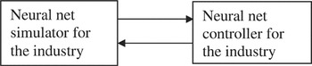
Our main goal in this research is to use the neuroevolution approach to control industries that work in real time. This paper basically shows how the neuroevolution technique can work as an industry controller to improve the whole system performance. This is done by applying an existing neuroevolution approach to be as an industrial controller and comparing the results with other well-known approaches (i.e., neural networks and simulation method). Because the ESP approach (and extensions of it) has been tested with various applications and proven its good performance, we choose it to be our approach for all sorts of problems (industrial problems) that have not been tested before with it. As noticed in the given background, most of the developed controllers are not concerned with industrial behaviors. We try in this paper to investigate and explore the ability of neuroevolutions in another application that has not been widely tested. To show our scheme performance, we apply it on two models. The first model is working as a linear function to control the temperature and humidity in an industry by increasing or decreasing its level based on the system/industry behavior (the temperature and humidity should always be moderate). The second model works as a nonlinear function to control scheduling in an industry. The industry has two queues for two machines that can manufacture different or the same parts. These two models will be explained in detail in the next section. In both the models, we have two neural networks: one to simulate the plant, and the other to control the plant. Figure 1 shows the general structure of any of the models.

The general structure to be used.
In both the models we use the following strategy:
1. First, construct a neural net to work as the industry simulator. Training of the net is done using backpropagation.
2. At random construct n number of controller neural nets. This is done by choosing random weights for each controller net. The input layer of the controller neural net consists of the input units to be controlled such as temperature or humidity. The inputs of the controller neural net is the output of the industry or the simulated neural network. The output layer of the controller neural net consists of the actions that should be as inputs for the industry (or the simulated neural net) to get the new temperature and humidity as an example.
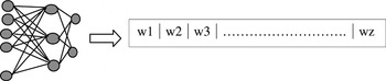
3. For each neural net used for control, its weights are coded as one chromosome as shown in Figure 2.
4. Do steps 5–6 n times.
5. For each neural net working as a controller, the system is tried for m number of times (cycle: from the simulator to the controller and vice versa) and its fitness value is computed.
6. Apply the genetic operators on the chromosomes. The applied genetic operators are
6.1. Crossover: two good chromosomes are chosen at random and two point crossover is applied. Two new nets will be produced.
6.2. Mutation: a chromosome is chosen at random in which we choose randomly a weight that is increased or decreased with a small real value.
6.3. The offspring is tried with the system for several iteration and its fitness value is computed.
6.4. Replace the obtained chromosomes (through the genetic operators) with other chromosomes that are less in fitness than them.
7. Choose the chromosome with the highest fitness value to work as a controller for the system.

The weights of the neural net represent one chromosome.
The reason behind coding the neural net in the way shown in Figure 2 is that it is the simplest way of coding and to make the easy application of genetic operators. This way of coding is the way used with ESP, which has proven good performance in various experiments. Another coding could be for each net; there are three different chromosomes: one for the input layer, the second for the hidden layer, and the last for the output layer. This makes the system implementation more complex even in genetic operators applications, but more useful than the first approach in cases where there is a good intuition (and not only randomness) about the starting weights of the neural net (for all the layers). Another way of coding could be the one used by NEAT, which has also proven a better performance than ESP in many experiments. NEAT coding is more complex than the one used in ESP. In NEAT, each genome includes a list of connection genes, each of which refers to two node genes being connected. Each connection gene specifies the in-node, the out-node, the weight of the connection, whether or not the connection gene is expressed, and innovation number, which allows finding the corresponding genes during crossover.
The genetic operators used are as those used with ESP and proven good performance. The crossover that is used is the two-point crossover (in ESP, this crossover is a one-point crossover), which, in general, will eventually give the same results as the one-point crossover or better, but the two-point crossover is used to give more opportunity to perform weight exchanges between the same layers in the two chosen nets (this is not very important in our case, but good to have it if possible). The mutation is exactly the same as used in ESP where the chosen weight is increased or decreased by a small real value.
3. THE MODELS
To observe our strategy on industries based on real-time systems, we applied it on two models. The first model is called a temperature–humidity controller, and the second model is called a scheduling controller. The first model is based on a linear function, whereas the second model is based on a nonlinear function. The two different models have been selected not only because they are different in terms of linearity, but also because they are totally different in their activities and controlling requirements, and each one of them will be compared with the results obtained by a traditional method.
3.1. Temperature–humidity controller
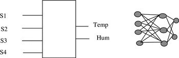
In this model we have a small unit in an industry that has four switches as inputs and two outputs that are temperature and humidity. The humidity and temperature in the industry should always be within certain range that we call moderate. The temperature and humidity values are obtained based on the input values for the switches. This problem seems to be simple in its structure; but, in fact, it is a real-life industrial controller problem that is common in various industries affected by temperature and humidity (such as stores or operations). This model is chosen for its reality and not for its simplicity. We have constructed a neural net to simulate the industry behavior. This is done using the backpropagation algorithm. Figure 3 shows the industry figure and the neural net used for simulation.

Industry of four input switches and two outputs, temperature and humidity. The neural net in the figure is a simulator for the industry.
Each switch value might be 1 or 0. Table 1 depicts the switches input values and the corresponding temperature and humidity values. Our concern is that the industry should always have a moderate temperature and moderate humidity, which is 0 < m ≤ 0.7, where m is the moderate value. Here, we have the role of the neural net controller obtained by neuroevolution. The controller should always modify the status of the switches whenever the temperature or the humidity does not cope with the industry environment. This means that the temperature and the humidity are the inputs for the controller net and the new switch values are the output values of the controller net. These output values will be the inputs for the simulator net.
The values of the switches of the industry and its corresponding temperature and humidity

The fitness function to be used for evaluating the controller net is based on the following:
- The temperature is 0 < temperature ≤ 0.7.
- The humidity is 0 < humidity ≤ 0.7.
A linear function for the system is also constructed to see the behavior of the system. These functions replace the values in Table 1. The proposed functions are as below:

and the moderate values for temperature and humidity are as below:
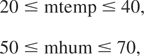
where mtemp is the moderate temperature and mhum is the moderate humidity. The value of X in the equations is the decimal value of the switch values related to either temperature or humidity. For example, if the switches s1 and s2 correspond to temperature, s3 and s4 correspond to humidity, and the values of s1 and s2 are 1 and 1, respectively, then X is 3 and the temp(X) will be 50. The fitness function used with linear functions is almost as explained for Table 1, with consideration for the range of the accepted temperature and humidity.
3.2. Scheduling controller
The idea of the industry to be considered here is taken from Drake and Smith (1996), with slight modifications to serve our purpose. In a workcenter we have two machines, m1 and m2. Each machine has its own queue, q1 and q2, for machines m1 and m2, respectively. Each queue has the part requests for manufacturing; each request can be represented by ri, which is the ith request. The workcenter can produce three types of parts, p1, p2, and p3; p1 can be produced by m1 or m2, whereas p2 can only be produced by m1; p3 can only be produced by m2; and m2 is faster than m1 by some percentage value. Figure 4 shows the workcenter.

Two machines m1 and m2 with two queues q1 and q2. For each machine there is a queue; m1 manufactures p2 parts, and m2 manufactures p3 parts, and p1 is manufactured by either m1 or m2.
Based on the current queues contents (number of requests) and the speed of each machine, the controller should decide what next part to be considered for the queues (what part type should send a request to take place in the queues). Moreover, the controller should decide what parts are chosen from the queues to be manufactured (it could be one part or two parts in parallel). The input for the simulation neural net is the next part to be allocated in the queues, which is obtained by the controller plus the queue contents. The output for the simulation neural net is the contents of the queues (in terms of the number of requests) after considering the new part and manufacturing one or two parts in parallel. The controller neural net is presented in Figure 5, and the workcenter simulator is presented in Figure 6. The decision of the controller (based on the fitness function) is based on the queue maximum size (we assume that the maximum size for both queues is the same), the speed of the machines, and the type of the part to be manufactured.

The neural net that works as a controller in the scheduling control model; q1 and q2 are the number of parts requests in each queue (queue1 and queue2). The next part type is 00, 01, 10, or 11; 00 and 11 (the parts that can be manufactured by both the machines) have the same meaning; 01 means the part can only be manufactured by m1, whereas 10 means the part can only be manufactured by m2; c1 and c2 have values 0 or 1; c1 is related to queue1; c2 is related to queue2; 1 means the queue will be reduced by 1, and this reduced part should be manufactured. This last step is called forced manufacturing for controlling purpose.

The neural net that works as a simulator for the workcenter. Its inputs are the outputs of the controller (with consideration to the number of requests in each of the queues) and its output is the new values of q1 and q2 after manufacturing and inserting a new part in one of the queues. The workcenter considers the new part in one of the queues and does a manufacturing based on the controller.
This controller model will work in a nonlinear manner because there is no direct relation between the inputs and outputs of the controller in terms of linearity. The system will eventually decide what is the proper queues movement that should be done to keep the stability of the industry. This decision is based on the fitness function. To clarify the fitness function used, we define some terms: (a) MAXQ is maximum value of queue contents; (b) cqi is the number of contents in the ith q; (c) r is the fast rate of m2 over m1; (d) np is the new part request obtained by the controller.
Following are the conditions that affect the fitness function that is used:
- (np = p1) AND (cq1 < MAXQ) AND (cq2 < MAXQ),
- (np = p2) AND (cq1 < MAXQ),
- (np = p3) AND (cq2 < MAXQ),
- (np = p1) AND (cq1 ≤ MAXQ AND cq2 ≤ MAXQ) AND (cq2 × r ≤ cq1).
4. EXPERIMENTAL RESULTS
In this section we present the results obtained by the neuroevolution schemes for controlling systems in the chosen models. We also compare the obtained results with traditional methods. In the temperature–humidity controller, we compare the obtained results with that obtained by a controller based on backpropagation neural networks. The results of the scheduling model is compared with the results obtained by a simulator proposed by Drake and Smith (1996) and used SIMAN V as a simulation language (we shall call this simulation system SA). In our system runs, we are concerned with the work of the controller to adjust the instability that might occur to the industry and how to deal with various situations.
4.1. Temperature–humidity controller
As explained in Section 3, in this model we are concerned with a controller that can always monitor the temperature and humidity of an industry based on four switches. Whenever (using the linear functions) the temperature goes below 20 or higher than 40; or the humidity goes below 50 or higher than 70, the controller should adjust the switches to bring back the industry to its stable status. Because the runs using Table 1 or the linear functions are giving almost the same impression, we shall show the results obtained using the linear functions. In this section, we shall show the obtained results from one of the several runs on the system. All the runs give the correct controller adjustments with a little variations (due to differences in weights between the nets), but still within the industry accepted ranges. The evolved controller net will decide by itself the values of the new switches that will adjust the temperature and humidity.
A snapshot for the controller work to adjust some unstable cases for the temperature and humidity is shown in Table 2. It is clear from Table 2 that whenever either the temperature or the humidity goes out of its range, the controller adjusts it (for sure by modifying the switches values). As explained in Section 3 the range of the temperature is 20–40 and the humidity is 50–70. From the table, we see that when the value 20–73 (temperature–humidity) is given, the controller will adjust it to 20–50 because of the humidity value (73 is above the accepted range). In the case of 30–69, which is itself stable because both values are within the accepted ranges, the controller still modify the values but again within the range. This is done because, in general, the controller cannot always produce the same values even if its inputs are within the accepted range, but surely it also gives values within the range.
Unstable cases of temperature and humidity and the corresponding controller adjustment

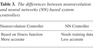
The same controller function has been implemented using neural networks based on the backpropagation algorithm. This is done to compare the obtained results and system requirements for both the approaches. Table 3 shows the main differences between the two approaches.
The differences between neuroevolution and neural networks (NN) based system controllers

One of the main differences is that in neuroevolution we do not need to prepare training examples, whereas using neural network (e.g., backpropagation) we need to get a training examples list. This is common, but the case here is that there is no fixed criteria to adjust the weights; for example, one of the training examples could have inputs 20–20 and the new switch values might give us results for the new temperature and humidity as 20–50, 30–60, 20–70, or any values within the accepted ranges for the temperature and humidity. This means for a certain input temperature and humidity, we might have various switch values. Using neuroevolution and based on the fitness function, the net itself will decide what the adjusted temperature and humidity should be, and we do not need to worry about providing training examples and how should the system will go with the improper values of temperature and humidity. This shows the advantages of using neuroevolution over neural networks.
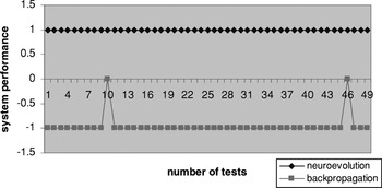
The second difference is that the results show that the controller using neuroevolution is more accurate than only using the neural networks. The accuracy with neuroevolution shows that it is 100% correct, whereas the accuracy with neural networks alone shows that it is 96%. This might be because in the net inputs we might have various output net switches (in which many are not given in the examples list). This result is expressed in Figure 7. Figure 7 shows the performance of the two controllers, neuroevolution controllers and the backpropagation-based controller. The 1 for the neuroevolution controller means that the controller gives a correct response, whereas the −1 for the backpropagation-based controller means that the controller gives a correct response. The 0 for both the controllers means that the controller gives a wrong response.

A comparison of the controller performance under neuroevolution and backpropagation.
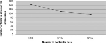
As expected, experiments show that the higher the number of the population (generated controller nets), the faster the system converges to solve all the given problems (in terms of the number of trials). Three populations of 50, 100, and 150 controller neural nets have been tested for the system. In every trial test we generate 20 arbitrary cases to be monitored by the controller. With 50 nets, the controller was able to adjust all the given cases after 143 trials, whereas with 100 and 150 nets, the controller was able to adjust all the given cases after 110 and 95 trials, respectively. Figure 8 shows that the higher the number of the population, the less the number of trials to adjust all the arbitrary states.

The higher the number of populations, the less the number of needed trials to adjust arbitrary cases (states).
4.2. Scheduling controller
In this section, we shall present the results obtained for applying the neuroevolution to the scheduling controller and compare these results with the results obtained by the simulation system proposed by Drake and Smith (1996), which we call SA. Comparing our obtained results with ordinary simulation method (such as SA) is very important because these methods are very common in control simulation. The neural network using backpropagation is not used for this problem because no examples are provided and the new part order to be considered for queuing is to be evolved based on the system performance. The behavior of this controlling model experiment is nonlinear. The developed controller is to decide what type of part order (request) should be issued based on the system behavior (depending on the queuing capacity and the time that the part request may stay in the queue). Moreover, the controller should also force and guide the system to take action in certain cases to manufacture certain parts (if things seem going smoothly, the controller will not force the system for manufacturing certain parts and the workcenter will work normally).
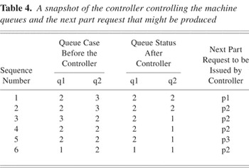
A snapshot for the controller system behavior is shown in Table 4. It is to be known that the needed variables are assigned the following values:
a. queue size: MAXQ = 3;
b. speed rate: how much m2 is faster than m1 (r = 0.5).
A snapshot of the controller controlling the machine queues and the next part request that might be produced

From Table 4 we follow a sequence of continuous steps as numbered. The first assumption is that the contents of queue1 and queue2 is 2 and 3, respectively. We shall use a q1–q2 representation, which means 2–3. The controller forces a manufacturing of one part of q2 resulting in 2–2, and proposes the next part request to be considered for queuing is of the type that can be manufactured by both the machines. The controller assigns q2 to allocate the request resulting in 2–3, then it forces the workcenter to manufacture another part from q2 and the new queues contents become 2–2. The controller also gives an order to receive a request that can be manufactured only by machine1. In step 3, we notice that we have 3–2, but the controller forces the workcenter to manufacture one by machine1 and another one by machine2, resulting in 2–1 and proposes a request that can be manufactured by only machine 1. From the results we can notice that almost every two parts manufactured using m2, one part is manufactured using m1. This is because the r chosen (the speed rate) of m2 is 0.5. It is also assumed that at the beginning of this run that there is a part in m1 and no parts in m2. It is to be noticed that the controller never proposes a part request for a full queue.
Using SA, the controller simulation was not designed to monitor the next part request for manufacturing (not as we proposed in our model), and was based on randomness. We added controlling the type of the request to expedite the process of the system and make harmony in queue-in and queue-out. Issuing part requests at random has an advantage, which may emulate the real industry, but controlling the issuing of part requests might be also useful to expedite and control the whole scheduling and management industry process. This is useful because these are decided based on each queue's size and the time needed for part manufacturing. This means that the system decides which part request it can accept based on its situation. Using randomness might issue a request that might need to wait because the corresponding queue is full. Moreover, in SA during scheduling, it checks if the queue of machine 2 contains more than the queue of machine 1, then it allocates the part request to machine 1, which is not always correct because machine 2 is faster than machine 1. Another variation is that because a neural network is used as an industry simulator, it can show the producing of manufactured two parts from the two machines at the same time, whereas using SA, it is difficult to show that. Figure 9 shows a comparison between the neuroevolution controller and the SA controller for 290 time units. After finishing the 290 time units the system using the neuroevolution controller was able to manufacture 204 parts, whereas using the SA controller, the system was able to manufacture 143 parts. This implies that the system that uses the neuroevolution controller is faster, with about 40% from that which uses the SA controller. This happened because the neuroevolution controller was also designed to control the type of part requests.

A comparison between the neuroevolution controller and the controller based on a simulation for the workcenter.
5. CONCLUSIONS
In this paper we presented an application of a neuroevolution strategy (ESP) to work as a controller for industries. The strategy has been applied on two models: a temperature–humidity controller, and a scheduling controller. In the temperature–humidity controller, the controller could very well adjust the industry switches to bring back the humidity and the temperature to their normal ranges. In the scheduling controller model, the controller could very well understand how the system should work, and significantly managed moving the part requests in and out from/to the queues based on the size of the queue and the speed of the corresponding machine. Based on the same factors, the controller could decide which part should send a request to be queued and wait for manufacturing. To evaluate the proposed scheme for the controllers, we compared the obtained results of the temperature–humidity controller using the neuroevolution with that of a controller based on neural networks, and also compared the obtained results of the scheduling controller using neuroevolution with that of a simulation of the controller developed by Drake and Smith (1996) using the SIMAN V simulation language. In both experiments, the neuroevolution approach shows better performance in terms of accuracy and goal achievement. According to our experiments and most of the previous experiments on applying neuroevolution to applications similar to ours, there is no direct clear limitation for such kind of systems. One of the important future directions could be exploring the weak points and drawbacks of such a system. To the contrary, such kinds of systems have clear advantage over the systems based only on neural networks or genetic algorithms alone. One clear thing is that the systems with a good set of examples would converge faster using backpropagation than with neuroevolution. This itself is not a limitation for the usage of neuroevolution because such approaches are basically used for cases where no examples are provided or the examples provided do not help in generalization. Some of the future directions could be applying neuroevolution approach on a real-life more complex real-time systems, or developing a system to distribute the time limit among the industry sensors to allow the controller to take the correct decision within time constraints. This could be done by making the system to decide which sensor is more important than the other based on the current industry situation (under research).
References
REFERENCES
Agogino, A.,
Stanley, K., &
Miikkulainen, R.
(2000).
Online interactive neuro-evolution.
Neural Processing Letters 11,
29–37.CrossRefGoogle Scholar
Conradie, A.,
Miikkulainen, R., &
Aldrich, C.
(2002).
Adaptive control utilizing neural swarming.
Proc. 2002 Genetic & Evolutionary Computation Conf.
(GECC-2002).
Drake, G. &
Smith, J.
(1996).
Simulation system for real-time planning, scheduling and
control.
Proc. 28th Conf. Winter Simulation, pp.
1083–1090.CrossRef
Fan, J.,
Lau, R., &
Miikkulainen, R.
(2003).
Utilizing domain knowledge in neuroevolution.
Proc. Twentieth Int. Conf. Machine Learning (ICML-03).
Florian, R.
(2004).
Evolution of Alternate Object Pushing in a Simulated Embodied Agent:
Preliminary Report.
Romania:
Center for Cognitive and Neural Studies (Coneural).
Gomez, F.
(2003).
Robust non-linear control through neuroevolution.
PhD Thesis.
University of Texas at Austin.
Gomez, F. &
Miikkulainen, R.
(2003).
Active guidance for a fitness rocket using neuroevolution.
Proc. Genetic Evolutionary Computation Conf.
(GECC-03).CrossRef
Gomez, F. &
Miikkulainen, R.
(2004).
Transfer of neuroevolved controllers in unstable domains.
Proc. Genetic Evolutionary Computation Conf. (GECCO
2004).CrossRef
Law, D. &
Miikkulainen, R.
(1994).
Grounding robotic control with genetic neural networks.
Technical Report AI-94-223. Austin, TX:
University of Texas at Austin, Department of of Computer
Sciences.
Nolfi, S. &
Floreano, D.
(2000).
Evolutionary Robotics.
Cambridge:
MIT Press.
Nolfi, S. &
Parisi, D.
(2002).
Evolution of artificial neural networks. In
Handbook of Brain Theory and Neural Networks
(Arbib, M., Ed.),
2nd ed., pp.
418–421.
Cambridge:
MIT Press.
Stanley, K. &
Miikkulainen, R.
(2002).
Efficient evolution of neural network topologies.
Proc. 2002 Congr. Evolutionary Computation
(CEC'02).CrossRef
Towell, G. &
Shavlik, J.
(1994).
Knowledge based artificial neural networks.
Artificial Intelligence 70,
119–165.CrossRefGoogle Scholar
Zhou, Z. &
Chen, S.
(2003).
Evolving fault-tolerant neural networks.
Neural Computing and Applications 11(3–4),
156–160.CrossRefGoogle Scholar
The general structure to be used.
The weights of the neural net represent one chromosome.
Industry of four input switches and two outputs, temperature and humidity. The neural net in the figure is a simulator for the industry.

The values of the switches of the industry and its corresponding temperature and humidity
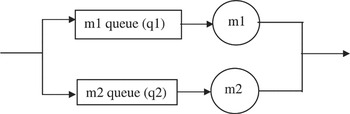
Two machines m1 and m2 with two queues q1 and q2. For each machine there is a queue; m1 manufactures p2 parts, and m2 manufactures p3 parts, and p1 is manufactured by either m1 or m2.
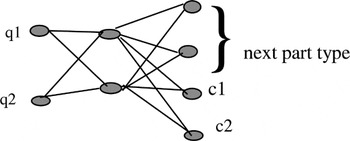
The neural net that works as a controller in the scheduling control model; q1 and q2 are the number of parts requests in each queue (queue1 and queue2). The next part type is 00, 01, 10, or 11; 00 and 11 (the parts that can be manufactured by both the machines) have the same meaning; 01 means the part can only be manufactured by m1, whereas 10 means the part can only be manufactured by m2; c1 and c2 have values 0 or 1; c1 is related to queue1; c2 is related to queue2; 1 means the queue will be reduced by 1, and this reduced part should be manufactured. This last step is called forced manufacturing for controlling purpose.
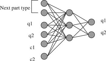
The neural net that works as a simulator for the workcenter. Its inputs are the outputs of the controller (with consideration to the number of requests in each of the queues) and its output is the new values of q1 and q2 after manufacturing and inserting a new part in one of the queues. The workcenter considers the new part in one of the queues and does a manufacturing based on the controller.
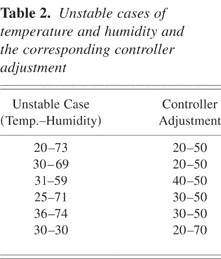
Unstable cases of temperature and humidity and the corresponding controller adjustment
The differences between neuroevolution and neural networks (NN) based system controllers
A comparison of the controller performance under neuroevolution and backpropagation.
The higher the number of populations, the less the number of needed trials to adjust arbitrary cases (states).
A snapshot of the controller controlling the machine queues and the next part request that might be produced
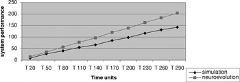
A comparison between the neuroevolution controller and the controller based on a simulation for the workcenter.
 You have
Access
- 2
- Cited by