1. INTRODUCTION
Consider the simple linear regression model

where x is the design variable taking values in (−∞,∞) and {εi} are the errors assumed to be independent and normally distributed with unknown variance σ2 > 0. For simplicity, we assume

. Our interest is point prediction of the response variable Y at a new value x0 ∈ (−∞,∞) of the design variable under the squared error loss.
Obviously, this is a simple statistical problem, even taught in introductory level statistical courses. Let

and

be the least squares estimators of α and β, respectively. Let f (x) = α + βx denote the true regression function. Then a predicted value of f (x0) is

. Under the simple linear regression model, it is the best unbiased estimator of f (x0) (under the squared error loss), and it is also a minimax estimator. Note that for a new observation Y0 at x0,

. Thus, as is well known, under the squared error loss, point prediction is equivalent to point estimation of f (x) at the given x value.
In many real applications, the linear relationship between x and Y is not obviously strong, and it is unclear whether β is zero (we note that, of course, the issue is the same if the concern is if β is equal to another constant instead of zero). The problem seems still simple, and again a solution is taught in elementary statistics courses: the familiar t-test. I imagine that this approach would be the one taken by many statisticians (if not most) in real applications (note that in reality, of course, the normality assumption has to be assessed). Some other statisticians may prefer the use of an information criterion for assessing if β = 0.
In the rather large literature on model selection, usually optimistic stories have been told. Theoretical results showed that, with a consistent model selection method, popular asymptotic properties (e.g., asymptotic normality and asymptotic efficiency) of estimators of interest are often unaffected (see, e.g., Pötscher, 1991). In contrast to such asymptotic analyses, initiated by Bancroft (1944), relatively few researchers have seriously examined finite-sample behaviors of estimators based on a selected model. In particular, when a preliminary test is used to choose a model before estimating a parameter, the resulting bias, risk, and admissibility of such an estimator were studied (see Judge and Bock, 1978; Judge and Yancey, 1986; Giles and Giles, 1993; Magnus, 1999; Magnus and Durbin, 1999; Danilov and Magnus, 2004, and references therein). The finite-sample distributions of such post-model-selection estimators have been derived also (see Leeb, 2005; Leeb and Pötscher, 2003). It was also shown that an asymptotic optimality property of the Akaike information criterion (AIC) in a nonparametric setting does not really mean that AIC is better than the Bayesian information criterion (BIC) (Kabaila, 2002). More recently, Leeb and Pötscher (2005) provided additional results and discussions on potential inappropriateness of asymptotic analysis for point and interval estimators based on model selection.
In this work, by focusing on the simple setting for a clear understanding of certain essential issues, we compare model selection methods in both theoretical and numerical investigations in the hope of complementing and strengthening the earlier realistic depictions of model selection methods and their relative performances.
2. A MOTIVATING NUMERICAL EXAMPLE
2.1. Setup
From the instructions in a typical elementary statistics textbook, when it is unclear if the slope parameter is nonzero, one should perform a hypothesis test. With the almost sacred choice of size 0.05, the familiar t-test can be used as a pre-test before estimating f.
Note that here we are dealing with two models, the simple linear model in (1) and the null model, Yi = α + εi, i = 1,2,…, n, with the same assumptions on the errors. For convenience, call them model 1 and model 0, respectively. Besides the preceding testing approach, we can use AIC or BIC to select one of them.
Let δA, δB, δT denote the procedures of estimating f (x) based on the outcome of AIC, BIC, and the testing (at the conventional size 0.05), respectively (the details will be given later in Section 3). Let Rβ(δ; x0; n) denote the mean squared error of the estimator

from an estimation procedure δ at the sample size n when the true slope parameter is β, i.e.,

. The risk does not depend on α for

based on a typical model selection method because of xn = 0, and its dependence on σ2 is suppressed because of our focus on the risk as a function of β (note that there is no need to consider different σ values: the change of the noise level simply rescales the risk plot).
Given that extensive work has been done theoretically and empirically on model selection and that our problem setting is one of the simplest possible, one may expect to see a fairly clear picture here. We start with a numerical investigation.
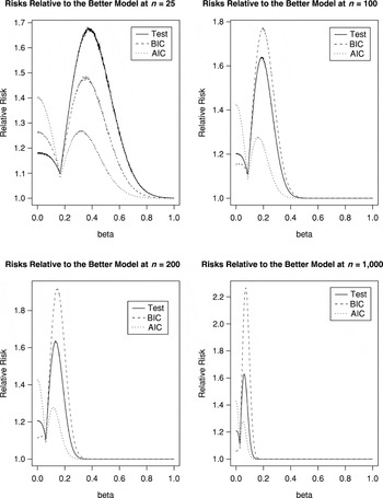
Consider an equally spaced design between [−1,1] with xn = 0 for prediction/estimation at x0 = 0.5. Figure 1 gives the risk functions of δA, δB, δT relative to the smaller of the two risks resulting from models 0 and 1 for β ≥ 0 at different sample sizes n = 25, 100, 200, and 1,000 with σ = 0.5. Note that at n = 25, δT is the least likely to select the larger model among the three methods, but when n ≥ 100, δB takes that role.

Comparing the model selection methods in risk at 4 sample sizes.
Before reading Figure 1 (we intentionally put Figure 1 on a different page), let's try to predict what we would expect to see. To that end, of course, the existing results on model selection are relevant and useful.
2.2. What Do the Most Well-Known Results Say?
In one sentence, a summary of the best known theoretical works on pointwise performance of AIC and BIC is perhaps something like “BIC is good if the true model is finite-dimensional, and AIC is good if the true model is infinite-dimensional.” This seems to be well supported. Indeed, when the true model is among the candidates, BIC is consistent in terms of selection (see, e.g., Nishii, 1984), and certain losses or risks of the estimator from BIC are asymptotically as small as they can be from the candidate models (Rissanen, 1986; Speed and Yu, 1993; Shao, 1997). When the true regression function is not in the candidate models, however, AIC has the so-called asymptotic efficiency property in estimating the regression function (see, e.g., Shibata, 1983; Li, 1987; Polyak and Tsybakov, 1991). Shao (1997) concluded that AIC and some other closely related criteria (such as Cp and delete-1 cross validation) are “useful when there is no fixed-dimensional correct model,” whereas BIC and delete-d cross validation with d/n → 1 are “useful in the case there exist fixed-dimensional correct models.”
In the debate on AIC and BIC, some researchers in favor of AIC argue strongly that there is no finite-dimensional “true model” (Burnham and Anderson, 2002). In defense of BIC, one can argue that in certain situations, some very simple models are clearly superior to nonparametric ones (imagine a simple linear regression with R2 close to 1) and then it clearly makes sense, practically speaking, to view one of the parametric models as the “true model.”
With the preceding understanding of the literature, I would have predicted the following results for the numerical experiment. (1) We expect three regions of β, β small, β large, and β in between, which correspond to BIC being better (while AIC is overfitting), AIC and BIC about the same, and AIC better (while BIC is underfitting). The first and third regions should shrink as n gets larger. (2) For this setting, from the literature, BIC should be favored in an overall sense.
Now let's examine Figure 1. Are there any surprises for you? To us, there were.
(1) Somewhat surprisingly, at n = 25, BIC loses to AIC at more β values and more severely compared to its shining moments.
(2) The worst case performance of BIC relative to AIC tends to get worse in n, even up to 1,000. In contrast, the worst case behavior of AIC relative to BIC seems to be confined.
What does the example tell us? When β is around zero, the advantage of BIC is relatively small (in risk), and the disadvantage of BIC is larger when β is larger. Thus it seems that BIC is paying a very high price for performing well at β around zero (as a result of being consistent in selection). Therefore, it seems fair to say that unless one has a strong reason to believe that β is around zero, the penalty of BIC is too large and thus is too conservative for yielding a good predictive performance. Considering the whole picture, even when n is large, the aforementioned optimality properties of BIC do not seem to reflect the reality well. The main reason, as will be seen later, is that the optimality properties are pointwise in nature and cannot be uniform in β.
For the testing approach, it also performs poorly, indicating that estimation/prediction is different from assessing if model 0 or model 1 is the true model at the size 0.05. We emphasize that the problem is not due to testing per se but is caused by the choice of significance level.
It should be pointed out that there have been a few underappreciated results in the literature on model selection that provide perspectives other than those given earlier. Indeed, the behavior that the worst case risk of BIC becomes increasingly worse compared to AIC was discovered by Foster and George (1994). Somewhat surprisingly, even though the risk inflation criterion (RIC) proposed in their paper is quite well known, as far as we know, this suboptimality of BIC has rarely been discussed. Kabaila (2002) pointed out that the pointwise asymptotic efficiency of AIC should not be interpreted as that AIC beats BIC when the sample size is large. Further concerns over misinterpretations of pointwise asymptotic results on model selection are provided in Leeb and Pötscher (2005). In particular, they emphasized that consistent model selection procedures actually do not allow one to apply the standard asymptotic distributions obtained without model selection. It is also useful to note that in real world statistical applications, practical aspects such as parsimony (see, e.g., Zhang, 1997) rather than asymptotic properties are often taken into consideration.
This paper grew out of our effort at trying to understand the properties of the model selection methods. The main points of this paper are as follows.
- For the purpose of estimation/prediction, we compare AIC and BIC from different theoretical angles to understand their differences. The theoretical results and the numerical comparisons show that the notion “BIC is good if the true model is finite-dimensional, and AIC is good if the true model is infinite-dimensional” is misleading.
- There is an unbridgeable difference between the pointwise and minimax properties of model selection. This means that no model selection method, however sophisticated, can share the essential strengths of AIC and BIC in risk.
- Large (e.g., BIC) and small (e.g., AIC) penalties in model selection are both justifiable from a weighted worst case risk point of view.
- We compare model selection and model averaging methods.
Some of the theoretical results given in this paper are not really original in the sense that similar results (under different loss functions) were given already in the literature. Our objective is to put these results and new ones into perspective, which hopefully will help the reader to understand the complex issues involved in model selection.
3. THEORETICAL COMPARISONS BETWEEN AIC AND BIC
3.1. A Brief Review of Model Selection Methods
The well-known t-test of size 0.05 is reject H0 if

where

is an unbiased estimator of σ2 and tn−2,0.025 is the cutoff point of the t distribution: P(tn−2 ≥ tn−2,0.025) = 0.025. With the outcome of the test, we can naturally make the following estimation:

Let

be the maximum likelihood estimator (MLE) of σ2 under model 1. Simple calculations show that BIC (Schwarz, 1978) selects model 1 when

Note that

is asymptotically equivalent to

. Replacing

by the estimator s in the last display (which has little effect when n is not small), we take the following slightly modified rule as BIC: select model 1 when
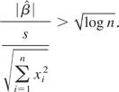
Similarly, AIC (Akaike, 1973) selects model 1 when

It is easy to see that

converges to

. Replacing

by s, we take the following modified rule as AIC: select model 1 when

Now AIC, BIC, and the testing approach all boil down to the decision of choosing model 1 when

with an being

,

, and tn−2,0.025, respectively. Thus in our context, AIC and BIC in a sense are also testing procedures: AIC has a size approaching 0.16 and BIC has a size approaching zero as n → ∞. Clearly, tn−2,0.025 approaches 1.96 as n → ∞, and when n is large, AIC is the most aggressive in terms of choosing the larger model and BIC is the most conservative, whereas the testing method is in between.
As is well known, the increasingly heavy penalty (or cutoff

in (2)) enables BIC to be consistent in terms of selecting the true model (i.e., model 0 if β = 0 and model 1 if β ≠ 0), whereas AIC and testing with a fixed size cannot avoid a nonvanishing probability of selecting the wrong model when β = 0.
In the rest of this section, we present theoretical comparisons between AIC and BIC from several different angles all under the consideration of the prediction/estimation risk at a given point x0.
3.2. A Pointwise Adaptation Result
Let

and

be two classes of functions. Consider two models:

and

Let

and

be estimators of f under models 0 and 1, respectively.
Consider a model selection rule δ. Let Aδ be the event that model 1 is selected.
Definition 1. The model selection rule δ is pointwise-risk adaptive with respect to the two estimators

and

if for all

and all x0 ∈ (−∞,∞) we have

as n → ∞.
In words, δ is pointwise-risk adaptive if for each given f in model 0 or 1, the estimator based on δ is asymptotically as good as the better one between

and

in risk. We use the term pointwise-risk to emphasize that the regression function f is fixed for the asymptotic analysis (as n → ∞).
Now in our simple context, let

and

. Note that when x0 = 0, the two estimators are actually the same.
THEOREM 1. Assume that the design is such that [sum ]xi2 is of order n as n → ∞. Then BIC is pointwise-risk adaptive with respect to

and

, but AIC is not. More generally, the model selection rule in (2) with

is pointwise-risk adaptive if and only if an → ∞.
Remarks.
- Results similar to Theorem 1 have been well known in the literature for general linear model selection, usually under the mean average squared error at the training sites. See, e.g., Nishii (1984), Shao (1997), and Leeb and Pötscher (2005). Speed and Yu (1993) give lower bounds for prediction risks and study achievability of the bounds by the familiar model selection criteria.
- AIC fails to be pointwise-risk adaptive when β = 0 because it selects (wrongly) model 1 with a nonvanishing probability no matter how large the sample size is.
- For each fixed β ≠ 0, the ratio of the risks of AIC and BIC converges to 1 as n → ∞.
- If
is not satisfied, the criterion has a nonvanishing probability of underfitting. See, e.g., Shao (1997) for a more general result on underfitting probability.

- The condition that [sum ]xi2 is of order n (i.e., [sum ]xi2/n is bounded between two positive constants) rules out highly irregular cases such as degeneration of the design points to a singleton.

Proof of Theorem 1. Consider x0 ≠ 0. For the model selection criterion with cutoff an, the corresponding estimator of f (x0) is

Let

. Then

Consider first the case β = 0, i.e., model 0 holds. Then clearly

is better than

, and their risks are σ2/n and

, respectively. For the model selection criterion to be pointwise-risk adaptive, we must have

(for x02 > 0). Because

and because β = 0,

has a standard normal distribution, we know that Pβ=0(Aδ) → 0 if and only if an → ∞. This fact is enough to rule AIC out as a pointwise-risk adaptive criterion. Because

has a standard normal distribution,

if Pβ=0(Aδ) → 0.
Now consider β ≠ 0. Without loss of generality, assume β > 0. When n is large enough,

is worse than

, and their risks are (σ2/n) + x02 β2 and

, respectively. Thus to show that the model selection criterion is pointwise-risk adaptive, we need to show that

But the quantity on the left-hand side is equal to

Note that for β ≠ 0,

converges in probability to β2 and it is not hard to show that, under the normality assumption on the errors,

holds if Pβ(Aδc) = o(n−1). Indeed,

where the last inequality follows from the Cauchy–Schwarz inequality. Together with the fact that

for some b > 0, the assertion follows. Now note that

With

, the last two probabilities are both exponentially small in n. This completes the proof of Theorem 1. █
3.3. Worst Case Performance
From Theorem 1, when β = 0, BIC beats AIC, and when β ≠ 0 AIC and BIC are asymptotically equivalent in pointwise risk as n → ∞. Together with the fact that BIC is consistent, it gives one a strong impression that BIC should be used for a parametric problem.
Obviously, there are various ways to compare the risk functions of estimation procedures. The asymptotics of Theorem 1 are done for each fixed f in the function classes. One drawback of this notion of asymptotics is that it tells very little for the specific data at hand because in general the convergence of the risk ratio in (3) is not uniform in f. An implication is that for a data set where the distinction between the two models is not clear because of small n or large noise (that is exactly where we need a good model selection rule most), it is especially uncertain whether the asymptotics are useful or not. A different notion to compare risk functions is in terms of worst case risk.
Let

be a class of regression functions. The minimax risk of estimating f (x0) is defined to be

where

is over all estimators based on the data.
Definition 2. A model selection rule δ is minimax-rate adaptive with respect to the two classes

and

if for both j = 0,1 and for all x0 ∈ (−∞,∞), we have

Theorem 2. Assume that the design is such that [sum ]xi2 is of order n as n → ∞. Then AIC is minimax-rate adaptive but BIC is not. More generally, the model selection rule δ of the form (2) is minimax-rate optimal if and only if an is bounded from above by a positive constant.
The theorem implies that in the least favorable case, AIC can only be finitely many times worse than BIC but the reverse is not true. This may be a little surprising. One may naturally think that because BIC is consistent, it will eventually select the true model. Together with its pointwise-risk adaptation property, it looks as if it should perform optimally at least in rate. Another thought may be that if I simply ignore model selection and use model 1 (the larger model), I always get the optimal rate of convergence. I probably should demand that BIC do at least as well as that.
A result similar to Theorem 2 was obtained by Foster and George (1994) in a linear regression setting assuming σ2 is known and under the average squared error at the training sites. Recently, Leeb and Pötscher (2005) derived a risk expression under a slightly different loss and obtained the same conclusion without the normality assumption on the errors.
Proof of Theorem 2. Note that the minimax rates of convergence for the two classes (i.e., linear functions and constant functions) are both n−1. With the same notations as in the proof of Theorem 1, we first show that for any an → ∞ and a fixed c > 0, we have

which is sufficient to conclude that when an → ∞, the model selection rule is minimax-rate suboptimal. Note that the left-hand side of the preceding expression is equal to

Observe that

Take

. It is easy to show that for any constant c′ > 1, P(s/σ ≥ c′ or s/σ ≤ 1/c′) converges to zero exponentially fast in n (i.e., P(s/σ ≥ c′ or s/σ ≤ 1/c′) = o(e−bn) for some b > 0; see, e.g., Yang, 1999, pp. 490–491). Note also that

and thus

. Then Pβn(Aδc) is asymptotically equivalent to

which approaches 1. Because nβn2 → ∞, we have nβn2Pβn(Aδc) → ∞. Therefore, an → ∞ implies that the worst case risk of the model selection estimator with cutoff an converges at a rate slower than n−1.
It remains to show that if an stays bounded, the resulting estimator converges at rate n−1. To that end, we need to show

Note that

, which is bounded from above. Consequently, it suffices to show that n supβ≥0 β2Pβ(Aδc) is bounded from above. Observe that

Thus

For |β| ≤ n−1/2, clearly nβ2Pβ(Aδc) is bounded from above by 2. For |β| > n−1/2, note that the two probabilities on the right-hand side in the preceding display decay exponentially fast in

. It follows easily that n supβ β2Pβ(Aδc) is indeed bounded from above. This completes the proof of Theorem 2. █
3.4. Comments on Theorems 1 and 2
Theorems 1 and 2 may seem to tell opposite stories. How do we interpret them? How do we use them to guide real applications if possible? Should one take the minimax or pointwise viewpoint?
In general, in our view, pointwise asymptotic results provide rather little guidance for real applications. For example, a theoretically elegant, universally consistent estimator in nonparametric regression with independent and identically distributed (i.i.d.) observations (i.e., it is consistent without any assumption on the common marginal distribution) may not perform well in practice even though theoretically it “works” universally. Pointwise asymptotics emphasize the positive outlook by assuming that we have a large number of observations for the current problem of interest. This is the case for some applications (think of many examples of simple linear regression in the elementary statistical textbooks) and perhaps can also be made the case sometimes when collecting more data is not a serious concern. In other situations, when one gets a larger sample size, it is usually desirable to consider more explanatory variables (which are usually available). For such a case, relevance and validity of the pointwise asymptotic analysis become less clear. It is perhaps worth pointing out that in the nonparametric world, pointwise asymptotics can be even less reliable in some sense. For example, super efficiency (i.e., the pointwise convergence rate is faster than the minimax rate) can occur at every function in an infinite-dimensional class of regression functions (see, e.g., Brown, Low, and Zhao, 1997). In any case, in a typical application where model selection is clearly a nontrivial issue, perhaps more often than not, we are not in a situation where the pointwise asymptotic behavior has already begun operating (or at least it is not evident that this is the case). To address this concern, properties such as minimaxity can be very helpful for better guiding the model selection practice.
Another comment is that whenever possible, we should try to understand/assess whether the difference in estimation/prediction that resulted from the different methods is really significant or not for the subject matter even if the statistical significance is obvious. Even though statistical significance is usually important, its practical relevance should be kept in mind in applications.
Nonuniformity of convergence of estimators based on model selection has been investigated by Leeb and Pötscher in several papers (see, e.g., Leeb and Pötscher, 2003, 2005) in different directions (such as estimating the distribution of estimators after model selection).
3.5. Can the Strengths of AIC and BIC Be Shared?
We have now seen the very distinct properties of AIC and BIC. Can we have a more sophisticated model selection method that can automatically behave like the better one of them in risk? It turns out that the contrast between pointwise and uniform convergence again shows up in answering this question. Indeed, as we show subsequently, in a pointwise sense, the strengths of AIC and BIC in risk can be combined; but once minimax rate is also sought, the picture is totally different.
3.5.1. Adaptive Pointwise Asymptotic Loss Efficiency.
One property that separates AIC and BIC is the condition under which a pointwise asymptotic loss efficiency (to be defined) holds. Shao (1997) showed that AIC (or a similar criterion) is pointwise asymptotically loss efficient when there is no fixed-dimensional correct model and BIC (or a similar criterion) is pointwise asymptotically efficient if there is a fixed-dimensional correct model. If one considers only the model selection criteria of the form

, where k is the model dimension,

is an estimator of σ2, and λn is the penalty coefficient (λn = 2 for AIC and λn = log n for BIC), then from Shao (1997), it is clear that any choice of λn cannot yield the pointwise asymptotic loss efficiency under both of the aforementioned conditions. This brings up an interesting question: Can we construct an adaptive model selection rule that does achieve the goal of pointwise asymptotic loss efficiency for both situations?
Under some conditions, we show that the answer is yes. Even though the rest of the paper focuses on the parametric case, we feel that this result is useful and interesting enough to be included here (at least in a sketchy way) for a good understanding of the model selection criteria. Again, we will not try to be general and prefer simplicity for seeing the essence more clearly.
Consider a collection of nested linear models with model index k ≥ 1, where k is simply the dimension of the model. The true model is

where xi = (xi1,…, xid) for some fixed d ≥ 1 and the errors are assumed to be independent and normally distributed with mean zero and known variance σ2 = 1. Let Mk = Mk,n denote the projection matrix of model k. Let fn = (f (x1),f (x2),…, f (xn))′ and Y = (Y1,…,Yn)′ be the vectors of the true values of the regression function at the design sites and the observations, respectively. Let

be the least squares estimator of fn based on model k. Let ∥·∥n denote the Euclidean distance on Rn.
Let δ be a model selection rule and let

be the selected model.
Definition 3. δ (or

) is said to be pointwise asymptotically loss efficient if

As mentioned already, AIC and BIC are pointwise asymptotically loss efficient for nonparametric and parametric cases, respectively, but not both (Shao, 1997). We need certain conditions to establish adaptive pointwise asymptotic loss efficiency.
When at least one of the candidate models is correct, a model selection rule is said to be strongly consistent if the selected model is eventually equal to the smallest correct model with probability one. For strong consistency of BIC for regression (under conditions on the design matrices), see Rao and Wu (1989). Related results are in Hannan and Quinn (1979), Geweke and Meese (1981), Pötscher (1989), and others.
Assumption 1. BIC is strongly consistent when at least one of the candidate models is correct.
Assumption 2. AIC is pointwise asymptotically loss efficient when none of the candidate models is correct.
Sufficient conditions for Assumption 2 are given by Shao (1997).
We now construct an adaptive model selection rule. Let

and

be the model selected by AIC and BIC, respectively, at sample size n. Let bn = max(3,[lfloor ]log log log n[rfloor ]) be an increasing sequence of integers. Let

The idea is very simple: when BIC selects the same model again and again at different sample sizes, the true model is most likely finite-dimensional, and hence BIC should be preferred.
For the strategy to work, we need some additional conditions for the nonparametric case. Let kn* = kAIC,n* be the minimizer of (1/n)∥ fn − Mk fn∥n2 + k/n over k ≥ 1. Note that kn* provides the best trade-off between the approximation error (1/n)∥ fn − Mk fn∥n2 and the estimation error k/n (recall that σ2 is assumed to be 1). We require the approximation errors to behave regularly in the following sense.
Assumption 3.
(1) If the approximation errors satisfy that for k ≥ 1,

for some constant c, then

(2) If the approximation errors satisfy that for k ≥ 1,

for some constant c, then

For interesting nonparametric regressions, it is usually the case that infk((1/n)∥ fn − Mk fn∥n2 + (k/n)) converges basically at (or around) a polynomial rate n−r for some 0 < r < 1, and then (4) is satisfied. Speed and Yu (1993) observed that when the approximation error rapidly decays at e−ek, AIC and BIC should perform the same in the sense

Note that the condition (5) is satisfied when the approximation error is ce−ek for the models. If the approximation errors behave regularly and of order O(e−ek) (including o(e−ek)), we expect it to continue to hold.
Proposition 1. For the model selection rule

,
(i) when (at least) one of the candidate models is correct, under Assumption 1,

is pointwise asymptotically loss efficient;
(ii) when none of the candidate models is correct, under Assumptions 2 and 3,

is pointwise asymptotically loss efficient.
The proposition states that under some reasonable conditions, an adaptive model selection rule can be pointwise asymptotically loss efficient for both parametric and nonparametric situations. However, because the result is in terms of pointwise asymptotic behavior, it gives an overly optimistic picture on capability of model selection when viewed from a more realistic perspective, as will be seen.
Proof of Proposition 1. To prove the result, it is sufficient to show that
(a) when at least one of the candidate models is correct,

will eventually equal to

almost surely;
(b) when the first condition of Assumption 3 holds, we have

;
(c) when the second condition of Assumption 3 holds, we have

The first one clearly holds with the strong consistency assumption on BIC. We next sketch the proof for the latter two cases.
Suppose that Assumption 3(1) holds. It suffices to show that

. Note that at the sample size bn,

. Thus it is sufficient to prove that

. Let kBIC,n* be the model that minimizes (1/n)∥ fn − Mk fn∥n2 + [k(log n − 1)/n] over k ≥ 1. Let Crit(k) = ∥Y − MkY ∥n2 + k log n be the BIC criterion value of model k (we only need to consider k ≤ n). Let en = (ε1,…, εn) and Ak = I − Mk, where I is the k × k identity matrix. Note that

where the last term ∥en∥n2 is irrelevant for model comparison because of its constant presence and independence of k. Under Assumption 3(1), for k ≤ bn, we have

for some c, and thus the remainder terms 2en′Ak fn and (k − en′Mk en) in the expression (6) are asymptotically negligible compared to ∥Ak fn∥n2. Similarly, for k = kBIC,n*, because kBIC,n* → ∞ as n → ∞ for the nonparametric case, we have that 2en′AkBIC,n* fn + (kBIC,n* − en′MkBIC,n* en) is asymptotically negligible compared to ∥AkBIC,n* fn∥n2 + kBIC,n*(log n − 1). Together with the assumption that ∥AkBIC,n* fn∥n2 + kBIC,n*(log n − 1) converges faster than n(log n)−1 for k ≤ bn and (7), we know that asymptotically Crit(k) > Crit(kBIC,n*) with increasingly high probability for k ≤ bn. Thus it is unlikely for

to be equal to

. Under the normality assumption, we have exponential probability bounds for the two remainder terms en′Ak fn and (k − en′Mk en), which can be used to easily make the preceding argument rigorous (see, e.g., the analysis in Yang, 1999, pp. 489–492).
Now we handle the remaining case when the approximation errors decay rapidly. When the approximation error is ce−ek, it can be shown that kBIC,n* satisfies that e−ekBIC,n* = o(kBIC,n*/n), and the same holds for kAIC,n*. Consequently the ratio

is asymptotically equal to the ratio of kBIC,n* and kAIC,n*, which can be easily verified to be approaching 1 as n → ∞. When the approximation errors converge faster than e−ek, we also have (1/n)∥ fn − MkBIC,n* fn∥n2 = o(kBIC,n*/n), and the same is true for AIC. Note that when the approximation error is regular, kBIC,n* is basically equivalent to kBIC,[lfloor ]n/log n[rfloor ]*. Hence the ratio in (8) converges to 1 under Assumption 3(2). One can also show that

in probability as n → ∞, and the same holds for BIC. This completes a sketched proof of the proposition. █
Remark. For the adaptive model selection rule

, it is not clear if it will eventually agree with AIC or BIC (whichever is the right one) with probability one. It is of interest to investigate if there exists any model selection rule that will eventually take AIC when none of the candidate models is correct and take BIC when at least one of the candidate models is correct.
3.5.2. No Model Selection Rule Can Be Really Adaptive between AIC and BIC.
Proposition 1 gives some hope of resolving the competition between AIC and BIC completely by sharing their strengths (it indeed succeeded in one aspect). Note that the adaptive pointwise asymptotic loss efficiency is a pointwise convergence property. How about other perspectives?
Theorem 2 shows that BIC pays a somewhat high price for being pointwise-risk adaptive in selection (or one can look at the issue from another angle: AIC pays a somewhat high price for being minimax-rate adaptive; i.e., it is not consistent in terms of selection). Naturally, one may wonder if this weakness of BIC can be overcome while maintaining its pointwise-risk adaptation property. In other words, is it possible to construct a more sophisticated model selection criterion that is both pointwise-risk adaptive and minimax-rate adaptive? If this can be done, then the debate between AIC and BIC is resolved to a large extent.
There are several attempts in the direction of combining strengths of AIC and BIC with positive results, including Barron, Yang, and Yu (1994) by applying the minimum description length criterion (MDL) (Rissanen, 1978) in a novel way to yield a penalty of AIC type or BIC type, whichever is better in risk; Hansen and Yu (1999) by taking a different application of MDL based on a pre-test; George and Foster (2000) by empirical Bayes approaches to have an adaptive penalty term; Rao and Tibshirani (1997) by adaptively choosing the penalty constant based on cross validation; Shen and Ye (2002) by using a generalized degree of freedom in the same direction of adaptively selecting the penalty constant.
Despite the positive findings, it turns out that the most essential risk properties of AIC and BIC cannot be combined. Consider the setting in Section 1.
Theorem 3. No model selection criterion can be both pointwise-risk adaptive and minimax-rate adaptive at the same time. Furthermore, for any model selection rule with the false selection probability under model 0 converging at order qn for some qn decreasing to zero, the worst case risk of the resulting estimator is at least of order (−log qn)/n.
Remark. The order (−log qn)/n is achieved by a model selection rule of the form (2) with an chosen such that the false selection probability (i.e., the probability of not selecting the true model) under β = 0 is of the specified order qn. From this angle, other model selection criteria cannot improve over those of the form (2) in terms of the worst case risk rate.
The theorem states that the main strengths of AIC and BIC in terms of risk cannot be combined. Thus pointwise-risk adaptation and minimax-rate adaptation are conflicting performance measures to some extent. The result is significant because it gives a clear answer to the fundamental question of how far adaptive model selection can really go.
In a closely related direction, Yang (2005) showed that in a linear regression setting with multiple candidate models, the consistency property of BIC and the minimax-rate adaptation property of AIC cannot be shared (note that a different loss, i.e., average squared error at the design points, is considered there). Relaxing the normality assumption, Leeb and Pötscher (2005, App. C) gave a similar result. Here in Theorem 3 the contrast is made between pointwise-risk adaptation and minimax-rate adaptation, and the result further characterizes the price one must pay in terms of the worst case performance for having the false selection probability go to zero. For a model selection rule of the form (2) with an → ∞, the worst case risk is at order an2/n. Note that fitting the larger model without any selection gives a risk of order 1/n.
Proof of Theorem 3. Consider a pointwise-risk adaptive model selection criterion δ. Let An be the event that model 1 is selected. From the proof of Theorem 2, to show that δ is not minimax-rate optimal, it suffices to show

Because δ is pointwise-risk adaptive, we have that when β = 0, for each x0 ∈ (−∞,∞),

and thus

Consequently, because the convergence holds for every x0, we must have

and

. Because under β = 0,

has a normal distribution with mean zero and variance σ2, we have Pβ=0(An) → 0 as n → ∞.
Consider a testing problem as follows. The observations are from the model

where the errors are independent and have standard normal distribution. Note that this corresponds to the case when α = 0. Consider testing H0 : β = 0 versus H1 : β > 0. If we take the rejection region An, δ becomes a testing rule with probability of type I error approaching zero. We next show, via the Neyman–Pearson lemma, that any test with the probability of type I error going to zero necessarily must have sup|β|≤c nβ2Pβ(Anc) → ∞. Let f (y1,…, yn;β) denote the joint probability density function of (Y1,…,Yn). Note that for β1 ≥ β0 ≥ 0,

Thus the family has a monotone likelihood ratio. It follows that a uniformly most powerful (UMP) test is to reject H0 when

is larger than some constant C. Let us choose the constant C = dn so that

. Let An,* denote the event of

. By the UMP property of An,*, we have for all β0 > 0, Pβ(An,*) ≥ Pβ(An). Consequently,

Now because

has normal distribution, it is easy to get

and for β > 0

Because

, we must have

(it can be easily shown that dn = o(n) for the probability of type II error to converge to zero). Then with the choice of

, we have

Because the last probability goes to 1 and ndn2/(4([sum ]xi2)2) → ∞, we have sup|β|≤c nβ2Pβ(An,*c) → ∞.
Now we prove the second part of the theorem. From the preceding discussion, we just need to show that ndn2/([sum ]xi2)2 is at least of order −log qn, where qn = Pβ=0(An). Note that

, where Φ denotes the standard normal cumulative distribution function. Let φ denote the standard normal probability density function. Because for t > 0,

(see e.g., Pollard, 2002, p. 317), it is easily shown that

is of order

. Consequently, ndn2/([sum ]xi2)2 is right at order −log qn. This completes the proof of Theorem 3. █
3.6. Subjectivity of the Choice of the Penalty in Model Selection
Note that under model 1, the least squares estimator gives

for estimating f (x). It has a constant risk

under the squared error loss. Assume that σ2 is known (or bounded from above by a known constant), so that the estimator

is in fact a minimax estimator. Because model 0 is contained in model 1, thus from a minimax point of view, this estimator cannot be improved. However, model selection comes into the picture because of the simple fact that when β is zero or small, the use of model 0 results in a much more accurate estimator/prediction. Clearly, insisting on the rigid minimax view is inappropriate because then the smaller model is always ignored. Foster and George (1994) proposed a risk inflation criterion to address this issue for linear regression. Later, George and Foster (2000) showed that different choices of the penalty (such as in AIC, BIC, and in between) can be derived from asymptotically maximizing the posterior probability under different choices of priors (allowing the priors to possibly depend on the sample size).
Here we show that different choices of the cutoff constant an in (2) are sensible depending on how one compares the risk functions of different methods. From this angle, different choices of penalty (or cutoff) are thus subjectively justifiable. We assign a prior probability on the models and weigh the worst case risks under the candidate models accordingly. Let π0 and π1 be the prior probabilities or weights on model 0 and model 1, respectively. Denote π = (π0,π1). Let

and

. For a model selection rule δ, let

be the weighted worst case risk.
We have the following natural definition to compare two model selection rules δ1 and δ2.
Definition 4. A model selection rule δ1 is said to be better than δ2 in terms of the weighted worst-case risk if R(δ1; x0; n;π) ≤ R(δ2; x0; n;π).
For each choice of π0 between 0 and 1, let a*(π) be the best choice of a that minimizes the weighted worst case risk among the class of model selection criteria given by (2). For the following result, for simplicity, we assume that σ2 is known to be 1 and assume that

. Accordingly the model selection criteria in (2) is changed to rejecting model 0 when

. Let δ{an} denote this selection rule.
Proposition 2. Let π0 > 0 and π1 > 0 and π0 + π1 = 1.
(i) If π is fixed, then AIC is better than BIC when n is large enough. In fact, for each fixed π,

for any {an} and {bn} with lim an = ∞ and lim sup bn bounded away from ∞.
(ii) For each fixed sample size, as π0 → 1, a*(π) → ∞.
From the first part of the result, giving model 0 a fixed positive prior probability is not enough for BIC to perform well from the weighted worst case risk point of view. The second part of Proposition 2 states that when model 1 is less likely to be true, the penalty should be larger for model 1, which clearly makes intuitive sense.
In the general linear regression context, it is natural to consider a class of criteria: choose the model that minimizes

where RSS is the residual sum of squares,

is an estimate of σ2, k is the dimension of the model, and λn is the penalty constant. It is called the GIC method in Rao and Wu (1989). Note that the issue of choosing λn is essentially the same as choosing an in (2) in our setting.
Clearly a choice of λn = λ > 2 is a compromise between AIC and BIC. However, under the average squared error, in terms of pointwise asymptotics, the criterion is not as good as AIC when the true model is infinite-dimensional and not as good as BIC when the true model is among the candidates (Shao, 1997, Sect. 3). Zhang (1997) in the discussion of Shao (1997) argues that any choice of λn = λ deserves consideration under a loss that weighs bias and variance differently from the squared error loss. The second part of Proposition 2 justifies a compromising criterion from our minimax point of view.
The proof of Proposition 2 is omitted.
4. AN ALTERNATIVE PENALTY CONSTANT FOR PREDICTION
In this section, we consider a simple alternative penalty constant (or cutoff) derived directly from the purpose of having a good risk function for estimation/prediction.
Recall that model 0 and model 1 have risk (σ2/n) + x02 β2 and

, respectively. Thus model 1 is better when

, i.e.,

Because β and σ are unknown, the preceding relationship cannot be directly used for choosing between model 0 and model 1. Obviously, we can try the plug-in approach of replacing the parameters by their estimates, respectively. Then a sensible model selection rule is to choose model 1 when

. This approach was studied in a more general regression framework in Toro-Vizcarrondo and Wallace (1968) and Wallace (1972) (see also Judge and Bock, 1978, pp. 53–55). Recognizing that the ratio

is a biased estimator of

, we may consider a modification when n is small. Because the numerator and the denominator are independent, the expectation is

. Observing that a multiple of s2/σ2 has a chi-square distribution, we can easily find that

. With this modification, we come to the criterion that selects model 1 when

We will denote this new selection rule δN. This criterion is even more aggressive in choosing model 1 than AIC (as n → ∞, the cutoff value

approaches 1 by Stirling's formula).
5. NUMERICAL RESULTS FOR COMPARING THE MODEL SELECTION METHODS
In this section, we present more numerical comparisons of the model selection methods.
First note that for a model selection rule of the form (2), by conditioning on s first, we have

Because

and s are independent, we have

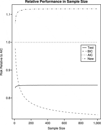
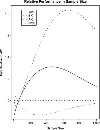
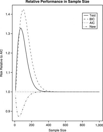
A similar expression is in Leeb and Pötscher (2005, Sect. 2.1). Thus as part of the computation of Rβ(δ; x0; n) for a model selection rule of the form (2), we can independently generate s2 (which basically has a chi-square distribution) a large number of times (we chose 2,000 in our computation) and then average the resulting values of the preceding expression. This is what we did when all the involved model selection rules are of the form (2) (Figures 1, 2, 3, and 4).

Comparing model selection methods from n = 10 to 1,000 at β = 0.

Comparing model selection methods from n = 10 to 1,000 at β = 0.2.

Comparing model selection methods from n = 10 to 1,000 at β = 0.5.
Here our interest is in knowing that, at a given value of the slope parameter β, how AIC, BIC, and the other methods compare to each other at different sample sizes. The asymptotic results in Section 3 have already told us that when n is very large, BIC is better than AIC when β = 0; and when β is nonzero, the risks of AIC and BIC are asymptotically equivalent.
Note that when n ≥ 8, BIC begins to have a cutoff an larger than AIC for model 1. In our simulation that follows, we consider sample sizes from 10 to 1,000. We choose σ = 0.5.
There are three scenarios, represented by three different values of β: β = 0,0.2,0.5. The plots of the risk functions relative to AIC are given in Figures 2, 3, and 4. When β = 0, BIC is better than AIC at all the sample sizes; when β = 0.2, in the beginning, BIC is better, but AIC becomes better with more observations; when β = 0.5, AIC is better right from the beginning. The second case (β = 0.2) indicates that if the sample size is not large enough to reasonably estimate β, it is better to pretend that it is zero. Note that even though in theory the risk ratio of AIC and BIC approaches 1 for the latter two cases, it has not quite happened when n is 1,000 for β = 0.2. This again suggests that the pointwise asymptotic optimality of BIC may not say much when the sample size is not very large (relative to β and σ2).
Regarding the new selection rule given in Section 4, it performs very well for relatively large β but poorly when β is small.
6. WHAT TO DO WHEN AIC AND BIC DISAGREE
For our simple setting, from (2), the disagreement between AIC and BIC indicates that the test statistic's value is neither large nor small (in absolute value). It is a case where the pointwise asymptotic behavior is questionable. The region of dispute for multiple model comparison becomes much more complicated. In any case, when the model selection criteria do disagree, the previous asymptotic results provide little hint on what to do. How should we address the issue?
Prior knowledge (hopefully not too subjective), if available, can be useful. For example, if historically β tends to be relatively small (or there is a good reason to believe so based on a subject matter theory) one should use BIC, and if no such information is available, it is better to use AIC for protection of the worst case performance. Note that when there are a number of explanatory variables, perhaps more often than not AIC and BIC select different models.
6.1. Combining the Models
When the model selection criteria do disagree on the data, as far as estimation/prediction is concerned, a solution to avoiding the pain of choosing the selection rules is a compromise: averaging the estimators from the models. Fortunately with an appropriate weighting of the models, the estimation accuracy can be substantially improved for such a situation.
Research has been done on general model averaging or model combining, including Bayesian approaches (for a review of the very rich works on Bayesian methods, see Hoeting, Madigan, Raftery, and Volinsky, 1999), frequentist approaches based on bootstrap or weighting via model selection criterion values (Breiman, 1996; Buckland, Burnham, and Augustin, 1997), and a method called ARM (adaptive regression by mixing) (Yang, 2001, 2003; Yuan and Yang, 2005). Magnus (2002) proposed the use of a Laplace prior for weighting estimates from different models in the problem of estimating the normal mean based on a single observation with known variance, which has a connection to a more general regression setting. In a simple case, Yang (2003) proved that model selection, no matter how sophisticated it is, is more than 25% worse than a combined estimator in an appropriate sense. Yang (2004) discusses two different directions of combining models (or general estimation procedures) with theoretical characterizations of their gains and prices they have to pay.
In general, model selection and model combining are both useful. Yuan and Yang (2005) showed that when model selection instability is high, model combining by ARM tends to do better or much better. But when model selection has little instability, model combining is not necessary, and it can even perform very poorly.
Next we give the ARM method (Yang, 2003) for our specific setting.
Step 1. Split the data into two parts Z(1) = (xi,Yi)i=1n/2 and Z(2) = (xi,Yi)i=n/2+1n.
Step 2. Estimate the parameters by the least squares method based on Z(1) for each model. Let

and

be the usual unbiased estimators of σ2 from model 0 and model 1, respectively (again based only on Z(1)).
Step 3. For each of the fitted models, assess the accuracies of the models using the remaining half of the data Z(2). Let D0 and D1 be the prediction sum of squares from model 0 and model 1, respectively.
Step 4. Compute the weight

Let W0 = 1 − W1.
Step 5. The combined estimate of f (x0) is

We consider an additional variant of ARM: it combines model 0 and model 1 as before only when AIC and BIC disagree with each other. We call it combining method 2.
6.2. Simulation and a Data Example
6.2.1. A Simulation.
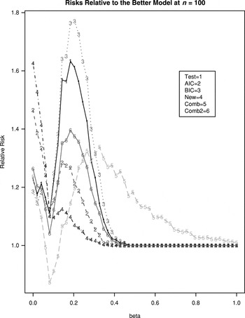
We now add the two combining methods in Section 6.1 to the list of the competing model selection methods in Section 5. The settings are kept the same. However, because we do not have simple expressions for the risks of the combined procedures, we simulate the risks of all the competitors based on 2,000 replications. Figure 5 gives the relative performance of the procedures compared to the better one of model 0 and model 1 at sample size 100. Recall that the risks of the least squares estimators from the two models are (σ2/n) + x02 β2 and

, respectively.

Comparing the selection/combining methods in β at n = 100.
From the graph, we do see performance improvement by the combining procedures when β is small (relative to the sample size). The combining procedure 1 always combines the two models and performs very well at the β values where the model selection methods differ most, yet it pays a heavy price when β is relatively large (when β is very large, it is fine). When the models are combined less aggressively by the second combining method (i.e., combining when AIC and BIC disagree), the problem of combining method 1 is substantially reduced (although it also gives up some advantage for small β). Overall, in our judgment, the combining method 2 does well.
6.2.2. A Data Example.
We demonstrate how the sample size n influences the relative performance of the model selection and model combining methods. The data set of body fat was used, which has 252 observations and 19 variables, and it was obtained from http://www.amstat.org/publications/jse/datasets/fat.txt.
Several problematic cases were removed following the comments by Johnson (1996). The new sample size is 247.
Unlike Penrose, Nelson, and Fisher (1985) and Johnson (1996), where the purpose of the analysis is to find predictive equations for the determination of body fat, our interest here is different, and we use only one predictor for simple linear regression.
The response variable is the percentage of body fat using Brozek's equation (the second variable in the data). The two individually used predictors are age and fat-free weight (original variables numbers 5 and 9). The correlation between the response and age is 0.293, and the correlation between the response and fat-free weight is −0.036. Roughly speaking, they correspond to two situations: the slope parameter is not small, and the slope parameter is very small or zero.
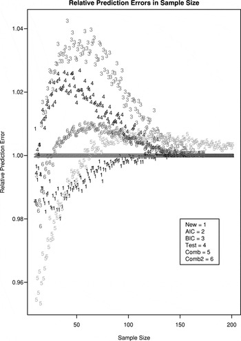
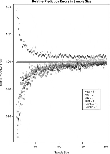
Figures 6 and 7 give the average prediction squared error of the model selection and model combining methods at sample sizes from 10 to 200. Note that at each sample size, we randomly split the whole data set with the first part of the size of the sample size and the second part used to compute the average prediction squared error. This is replicated 200 times. The performances of the methods given in the figures are all relative to the performance of AIC.

Empirical comparison of predictive performances at different sample sizes: Age as the predictor.

Empirical comparison of predictive performances at different sample sizes: Fat-free weight as the predictor.
The results are very interesting and confirm our earlier understanding. For the first case with age as the predictor, from the entire data set, we know that the slope parameter is nonzero and not very small (relatively speaking). When the sample size is around 10, BIC performs better but soon becomes worse than AIC. It continues to worsen and then comes back and eventually performs about the same compared to AIC. Note that the pointwise-risk adaptivity of BIC assures that in the preceding situation, BIC will eventually perform as well as AIC. For the second case with fat-free weight as the predictor, the slope parameter is very small (relative to the sample sizes), and we expect BIC to be better. That is indeed the case. As the sample size increases, their difference become smaller in the ratio. From Figure 7, at the end, AIC and BIC perform quite similarly. From the earlier theory, if the slope parameter is really zero, then the gap between AIC and BIC will never be closed. On the other hand, if we had a sample size of 10,000 (say) instead of 247, the observed correlation of −0.036 is no longer negligible, and we would see that AIC and BIC cross position with AIC being better as the sample size increases and then eventually the performance ratio going to 1. It is worth pointing out that comparing the two figures, we see that for a much wider range in case 1, BIC is significantly worse than AIC.
The test approach is between AIC and BIC, performing better than BIC in case 1 but worse for case 2. Overall, it seems that the testing approach is better than BIC.
The new selection rule goes opposite to the testing approach and BIC.
Finally, but not least, the two combining procedures work both very well, except for the first combining procedure with large sample sizes, where the model selection procedures have little difficulty finding the better model. The approach of combining the models when AIC and BIC disagree is perhaps the overall winner among the competitors.
In our view, when there is little prior experience on the slope parameter, combining the models is a good approach for prediction when model selection methods give different answers.
7. CONCLUDING REMARKS
In this work, with both theoretical examinations and numerical demonstrations, it is seen that the popular notion of preferring BIC for parametric regression is misleading. The pointwise asymptotic optimality properties of BIC (or any other consistent model selection method) are often interpreted overly optimistically in the current statistical literature. From the numerical results, it is also clear that the method of testing a hypothesis (at a conventional significance level) first and then making a prediction/estimation should not be the one students learn implicitly or explicitly from our future statistics textbooks. Although adaptive model selection with a data dependent penalty can be very helpful to reduce risk, it simply cannot integrate the pointwise optimality property of BIC and the minimax-rate optimality of AIC.
When model selection rules give very different answers, model combining is a better alternative approach for estimation/prediction. With proper weighting, the large variability of the estimator from model selection can be substantially reduced. Numerical results in this work show that combining the models when AIC and BIC disagree gives improved overall performance.
In real applications, it is often desirable to try different kinds of models. When a large number of models are in competition, however, model selection bias can be severe. For results dealing with this issue, see Barron and Cover (1991), Yang and Barron (1998), Yang (1999), Barron, Birgé, and Massart (1999), and Birgé and Massart (2001).