Tett, Hundley, and Christiansen (Reference Tett, Hundley and Christiansen2017) raise an important issue related to meta-analysis and our frequent overinterpretation of point estimates to the diminishment of variability of the estimate. We view this as analogous to the situation in which weather forecasters communicate the likely track of hurricanes. Such predictions involve point estimates of where the center of the storm is likely to be at some future time. These point estimates can be connected to identify the most likely path of the storm. In addition to these point estimates, however, forecasters caution that we should also attend to the “cone of uncertainty.” That is, we should not focus exclusively on the point estimate to the exclusion of the errors of prediction.
In this commentary, we extend Tett et al.’s (Reference Tett, Hundley and Christiansen2017) argument by identifying an additional source of variability in meta-analysis: uncertainty with respect to SDρ
. Greater attention to the between-study variance of effect sizes brings with it a need to consider the precision of our estimates of SDρ
. Although it is common, if not obligatory, to consider sampling error in estimates of the mean effect size, researchers frequently overlook the degree of uncertainty in our statistics when evaluating between-study heterogeneity. We build confidence intervals and credibility intervals around the mean correlation, but we give little thought to our uncertainty regarding the endpoints of the intervals (Evangelou, Ioannidis, & Patsopoulos, Reference Evangelou, Ioannidis and Patsopoulos2007).
Precision of SDρ
Estimates
Two approaches exist for evaluating sampling error in between-study heterogeneity statistics. First, we can test the between-study variance for statistical significance, using Hedges Q-test (Hedges & Olkin, Reference Hedges and Olkin1985). As a significance test, this approach indicates that SDρ
is greater than zero (if significant) or that we cannot rule out zero variance as a possibility (if nonsignificant). Unfortunately, neither of these conclusions is entirely satisfactory. If significant, we still do not know how much faith to place in our estimate of SDρ
. If nonsignificant, the result is inherently ambiguous in situations with small K, because the test tends to have lower power unless the number of studies is large (Hedges & Vevea, Reference Hedges and Vevea1998).
The second approach is to build a confidence interval around the variance estimate. Confidence intervals are generally favored over significance tests because (a) statistical significance can be inferred when the confidence interval does not include zero, and (b) confidence intervals appropriately present heterogeneity as ranging on a continuum rather than simply being present or absent (i.e., dichotomous thinking; Cumming & Fidler, Reference Cumming and Fidler2009). Several methods for constructing confidence intervals on between-study variance have been developed (Borenstein, Hedges, Higgins, & Rothstein, Reference Borenstein, Hedges, Higgins and Rothstein2009; Brannick & Hall, Reference Brannick, Hall and Brannick2003; Viechtbauer, Reference Viechtbauer2005, Reference Viechtbauer2007). These methods build a confidence interval around the between-study variance rather than SDρ
; however, the square root of the resulting endpoints can be used to represent an interval around SDρ
(Borenstein et al., Reference Borenstein, Hedges, Higgins and Rothstein2009). Confidence intervals can also be constructed around the I
2 statistic (Higgins & Thompson, Reference Higgins and Thompson2002), which quantifies the degree of heterogeneity as the proportion of between-study variance to total variance. Pragmatically, the R package metafor (Viechtbauer, Reference Viechtbauer2010) provides confidence intervals around VARρ
, SDρ
, and I
2.
In many situations, examining confidence intervals around SDρ
is likely to reveal substantial uncertainty in the degree of between-study variance. Credibility intervals can be quite large, even when the true SDρ
equals zero (Oswald & Johnson, Reference Oswald and Johnson1998). This is particularly true when examining moderator subgroups, which often rely on a fairly small number of studies.
To illustrate, Morris, Daisley, Wheeler, and Boyer (Reference Morris, Daisley, Wheeler and Boyer2015) reported a random-effects meta-analysis on the validity of individual psychological assessments, with an average uncorrected validity of .27 predicting job performance ratings. SDρ
was estimated at .12, indicating substantial variability across studies (i.e., an 80% credibility interval of .12 to .42). Using metafor, the current authors estimated a 95% confidence interval for SDρ
ranging from .078 to .192. Further, the confidence interval on the I
2 statistic indicated that between 41% and 81% of the observed variance was due to true between-study differences.
The impact of the uncertainty in the SDρ
estimate can be seen by constructing alternate credibility intervals using the endpoints of the SDρ
confidence interval. At the lower end (SDρ
= .078), the 80% credibility interval would be .27 ± 1.28 * .078, ranging from .17 to .37, and suggests relatively minor differences in validity between studies. Using the upper bound estimate, however, resulted in an 80% credibility interval (.27 ± 1.28 * .192) that ranged from .02 to .52, implying strikingly different levels of validity across different settings.
So, what can we conclude from these results? Validity is not homogenous, and there is some degree of situation specificity present in these data. However, the extent of this variability is quite uncertain. We simply do not have enough data with 37 samples to accurately estimate the likely range of validities.
Effects of K on the Precision of SDρ
In their focal article, Tett et al. (Reference Tett, Hundley and Christiansen2017) draw attention to the paradoxical association between increased situational specificity and the corresponding decrease in certainty around estimates of ρ and VARρ
(i.e., SD
2
ρ) as a function of K. It is similarly important to recognize how K influences the precision of confidence intervals around our estimates of heterogeneity.
As noted, there are several methods for constructing confidence intervals around SDρ
(see Viechtbauer, Reference Viechtbauer2007). For ease of demonstration, we focus on the Wald-type confidence interval, for which the role of K is most transparent. First, we estimate the sampling variance of SD
2
ρ,
where SD
2
ρ is the between-studies variance estimate, and σ2
j
is the within-study variance estimate. Once this estimate is obtained, a confidence interval for SD
2
ρ can be constructed as:
A 95% confidence interval for SDρ
is then obtained by calculating the square root of the upper and lower confidence limits for SD
2
ρ. Typically, lower confidence limits that fall below zero are truncated to zero (Viechtbauer, Reference Viechtbauer2007).
To see the effect of K, assume that the within-study variance is constant such that σ2
j
= σ
e
2. Once we make this substitution, Equation (1) simplifies to:
Thus, for given values of SDρ
and σ2
e
, as K decreases, the width of the confidence interval around SDρ
increases.
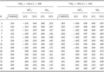
Table 1 presents a brief demonstration of the effects of K on the confidence interval for SDρ
for two levels of heterogeneity. On the left, we present the results for the estimates of SDρ
and the average estimate of σ2
j
(referred to below as σ2
e
) obtained from Morris et al. (Reference Morris, Daisley, Wheeler and Boyer2015). The degree of heterogeneity in the Morris et al. study is fairly large, and as Tett et al. note, the magnitude of SDρ
is likely to decrease as the analysis focuses on more specific situations (i.e., moderator subgroups). Therefore, on the right side of Table 1, we present the findings for smaller estimates of SDρ
and σ2
e
, representing likely values for more narrowly focused situations (Tett et al., Reference Tett, Hundley and Christiansen2017). As shown in Table 1, for a given level of SDρ
and σ2
e
, the width of the confidence interval decreases as K increases. Notice, however, that this pattern is stronger for the larger estimates of SDρ
and σ2
e
. As such, the influence of K on the confidence interval for SDρ
is stronger where there is greater heterogeneity around the effects.
Table 1.
Effect of K on 95% Confidence Intervals for SDρ
Recommendations
Our primary motivation in offering this commentary is to reify the point made by Tett et al. (Reference Tett, Hundley and Christiansen2017) regarding the need for greater attention to the variability of our estimates. In the context of meta-analysis, we recommend that researchers report confidence intervals around SDρ
and incorporate this into their discussion of results. More broadly, we encourage researchers to comprehensively and accurately report and interpret the degree of (un)certainty in results across all analyses.




 You have
Access
Tett, Hundley, and Christiansen (Reference Tett, Hundley and Christiansen2017) raise an important issue related to meta-analysis and our frequent overinterpretation of point estimates to the diminishment of variability of the estimate. We view this as analogous to the situation in which weather forecasters communicate the likely track of hurricanes. Such predictions involve point estimates of where the center of the storm is likely to be at some future time. These point estimates can be connected to identify the most likely path of the storm. In addition to these point estimates, however, forecasters caution that we should also attend to the “cone of uncertainty.” That is, we should not focus exclusively on the point estimate to the exclusion of the errors of prediction.
In this commentary, we extend Tett et al.’s (Reference Tett, Hundley and Christiansen2017) argument by identifying an additional source of variability in meta-analysis: uncertainty with respect to SDρ . Greater attention to the between-study variance of effect sizes brings with it a need to consider the precision of our estimates of SDρ . Although it is common, if not obligatory, to consider sampling error in estimates of the mean effect size, researchers frequently overlook the degree of uncertainty in our statistics when evaluating between-study heterogeneity. We build confidence intervals and credibility intervals around the mean correlation, but we give little thought to our uncertainty regarding the endpoints of the intervals (Evangelou, Ioannidis, & Patsopoulos, Reference Evangelou, Ioannidis and Patsopoulos2007).
Precision of SDρ Estimates
Two approaches exist for evaluating sampling error in between-study heterogeneity statistics. First, we can test the between-study variance for statistical significance, using Hedges Q-test (Hedges & Olkin, Reference Hedges and Olkin1985). As a significance test, this approach indicates that SDρ is greater than zero (if significant) or that we cannot rule out zero variance as a possibility (if nonsignificant). Unfortunately, neither of these conclusions is entirely satisfactory. If significant, we still do not know how much faith to place in our estimate of SDρ . If nonsignificant, the result is inherently ambiguous in situations with small K, because the test tends to have lower power unless the number of studies is large (Hedges & Vevea, Reference Hedges and Vevea1998).
The second approach is to build a confidence interval around the variance estimate. Confidence intervals are generally favored over significance tests because (a) statistical significance can be inferred when the confidence interval does not include zero, and (b) confidence intervals appropriately present heterogeneity as ranging on a continuum rather than simply being present or absent (i.e., dichotomous thinking; Cumming & Fidler, Reference Cumming and Fidler2009). Several methods for constructing confidence intervals on between-study variance have been developed (Borenstein, Hedges, Higgins, & Rothstein, Reference Borenstein, Hedges, Higgins and Rothstein2009; Brannick & Hall, Reference Brannick, Hall and Brannick2003; Viechtbauer, Reference Viechtbauer2005, Reference Viechtbauer2007). These methods build a confidence interval around the between-study variance rather than SDρ ; however, the square root of the resulting endpoints can be used to represent an interval around SDρ (Borenstein et al., Reference Borenstein, Hedges, Higgins and Rothstein2009). Confidence intervals can also be constructed around the I 2 statistic (Higgins & Thompson, Reference Higgins and Thompson2002), which quantifies the degree of heterogeneity as the proportion of between-study variance to total variance. Pragmatically, the R package metafor (Viechtbauer, Reference Viechtbauer2010) provides confidence intervals around VARρ , SDρ , and I 2.
In many situations, examining confidence intervals around SDρ is likely to reveal substantial uncertainty in the degree of between-study variance. Credibility intervals can be quite large, even when the true SDρ equals zero (Oswald & Johnson, Reference Oswald and Johnson1998). This is particularly true when examining moderator subgroups, which often rely on a fairly small number of studies.
To illustrate, Morris, Daisley, Wheeler, and Boyer (Reference Morris, Daisley, Wheeler and Boyer2015) reported a random-effects meta-analysis on the validity of individual psychological assessments, with an average uncorrected validity of .27 predicting job performance ratings. SDρ was estimated at .12, indicating substantial variability across studies (i.e., an 80% credibility interval of .12 to .42). Using metafor, the current authors estimated a 95% confidence interval for SDρ ranging from .078 to .192. Further, the confidence interval on the I 2 statistic indicated that between 41% and 81% of the observed variance was due to true between-study differences.
The impact of the uncertainty in the SDρ estimate can be seen by constructing alternate credibility intervals using the endpoints of the SDρ confidence interval. At the lower end (SDρ = .078), the 80% credibility interval would be .27 ± 1.28 * .078, ranging from .17 to .37, and suggests relatively minor differences in validity between studies. Using the upper bound estimate, however, resulted in an 80% credibility interval (.27 ± 1.28 * .192) that ranged from .02 to .52, implying strikingly different levels of validity across different settings.
So, what can we conclude from these results? Validity is not homogenous, and there is some degree of situation specificity present in these data. However, the extent of this variability is quite uncertain. We simply do not have enough data with 37 samples to accurately estimate the likely range of validities.
Effects of K on the Precision of SDρ
In their focal article, Tett et al. (Reference Tett, Hundley and Christiansen2017) draw attention to the paradoxical association between increased situational specificity and the corresponding decrease in certainty around estimates of ρ and VARρ (i.e., SD 2 ρ) as a function of K. It is similarly important to recognize how K influences the precision of confidence intervals around our estimates of heterogeneity.
As noted, there are several methods for constructing confidence intervals around SDρ (see Viechtbauer, Reference Viechtbauer2007). For ease of demonstration, we focus on the Wald-type confidence interval, for which the role of K is most transparent. First, we estimate the sampling variance of SD 2 ρ,
where SD 2 ρ is the between-studies variance estimate, and σ2 j is the within-study variance estimate. Once this estimate is obtained, a confidence interval for SD 2 ρ can be constructed as:
A 95% confidence interval for SDρ is then obtained by calculating the square root of the upper and lower confidence limits for SD 2 ρ. Typically, lower confidence limits that fall below zero are truncated to zero (Viechtbauer, Reference Viechtbauer2007).
To see the effect of K, assume that the within-study variance is constant such that σ2 j = σ e 2. Once we make this substitution, Equation (1) simplifies to:
Thus, for given values of SDρ and σ2 e , as K decreases, the width of the confidence interval around SDρ increases.
Table 1 presents a brief demonstration of the effects of K on the confidence interval for SDρ for two levels of heterogeneity. On the left, we present the results for the estimates of SDρ and the average estimate of σ2 j (referred to below as σ2 e ) obtained from Morris et al. (Reference Morris, Daisley, Wheeler and Boyer2015). The degree of heterogeneity in the Morris et al. study is fairly large, and as Tett et al. note, the magnitude of SDρ is likely to decrease as the analysis focuses on more specific situations (i.e., moderator subgroups). Therefore, on the right side of Table 1, we present the findings for smaller estimates of SDρ and σ2 e , representing likely values for more narrowly focused situations (Tett et al., Reference Tett, Hundley and Christiansen2017). As shown in Table 1, for a given level of SDρ and σ2 e , the width of the confidence interval decreases as K increases. Notice, however, that this pattern is stronger for the larger estimates of SDρ and σ2 e . As such, the influence of K on the confidence interval for SDρ is stronger where there is greater heterogeneity around the effects.
Effect of K on 95% Confidence Intervals for SDρ
Note. LCL = lower 95% confidence limit, UCL = upper 95% confidence limit. aValues from Morris et al. (Reference Morris, Daisley, Wheeler and Boyer2015). bLikely values for more narrow situations, as represented in Tett et al. (Reference Tett, Hundley and Christiansen2017).
Recommendations
Our primary motivation in offering this commentary is to reify the point made by Tett et al. (Reference Tett, Hundley and Christiansen2017) regarding the need for greater attention to the variability of our estimates. In the context of meta-analysis, we recommend that researchers report confidence intervals around SDρ and incorporate this into their discussion of results. More broadly, we encourage researchers to comprehensively and accurately report and interpret the degree of (un)certainty in results across all analyses.