1. Introduction
The issue of boundary layer transition has long been a significant yet challenging research topic. With the ongoing advancement of high-speed flight technology, comprehending the boundary layer transition mechanism becomes crucially important, since the boundary layer transition can yield a substantial rise in wall friction and thermal load.
Distributions of primary and secondary disturbance frequencies and wavenumbers in (a) the fundamental resonance of the K-type transition, (b) the subharmonic resonance of the N-type transition and (c) the O-type transition. The red, blue and white symbols denote the primary modes, travelling secondary modes and stationary streaks, respectively.

The transition paths and mechanisms of boundary layers are highly diverse, influenced significantly by the amplitude of incoming flow disturbances. Early studies (Herbert Reference Herbert1988; Kachanov Reference Kachanov1994; Schmid & Henningson Reference Schmid and Henningson2012) predominantly centred on incompressible boundary layers, unveiling a variety of transition scenarios. Figure 1 illustrates the schematic diagram of the frequencies and wavenumbers for the weakly nonlinear transition mechanisms of three representative scenarios. These categories correspond to different nonlinear interaction mechanisms involving a pair of oblique waves with the opposite wave angles and/or a planar wave.
For supersonic flows, the oblique first mode is most unstable, leading to a strong oblique breakdown constituted by a pair of oblique first modes (Chang & Malik Reference Chang and Malik1994). In the high-Mach-number regime, the planar Mack second mode dominates, favouring both the fundamental resonance (Sivasubramanian & Fasel Reference Sivasubramanian and Fasel2015) and the combination resonance (Chen, Zhu & Lee Reference Chen, Zhu and Lee2017). By contrast, subharmonic resonance is generally considered to be relatively weak. Additionally, the interaction between the oblique second mode and oblique waves can facilitate energy transfer via the parametric resonance process of difference modes (Zhou et al. Reference Zhou, Liu, Lu and Yan2023). Furthermore, the coupling of multiple dominant modes can also accelerate the transition process through interactions involving higher harmonics (Jahanbakhshi & Zaki Reference Jahanbakhshi and Zaki2019; Guo, Hao & Wen Reference Guo, Hao and Wen2023).
Compared with the two-dimensional (2-D) counterpart, three-dimensional (3-D) boundary layers feature three specific regions, i.e. the attachment-line, cross-flow and streamwise vortex regions, owing to the azimuthal pressure gradient (Chen et al. Reference Chen, Dong, Tu, Yuan and Chen2022). For supersonic boundary layers, the attachment line region exhibits instability modes similar to those of two-dimensional boundary layers (Fedorov & Egorov Reference Fedorov and Egorov2022). A recent study (Chen et al. Reference Chen, Dong, Tu, Yuan and Chen2023) demonstrates global Mack modes can spontaneously trigger the fundamental resonance. The cross-flow region is susceptible to cross-flow instability disturbances that, with sufficiently large amplitudes, are prone to secondary instabilities responsible for the final breakdown of the boundary layer (Craig & Saric Reference Craig and Saric2016; Moyes et al. Reference Moyes, Paredes, Kocian and Reed2017; Xu et al. Reference Xu, Chen, Liu, Dong and Fu2019). Recently, Ren & Kloker (Reference Ren and Kloker2022) analysed cross-flow instabilities in non-ideal gases, finding that wall heating destabilises cross-flow instabilities in the supercritical regime, whereas the supercritical and subcritical regimes show opposite wall-temperature effects relative to ideal gases and liquids. Similarly, the streamwise vortex region features a (pair of) large-scale streamwise vortex (vortices) accompanied by low-speed streaky structures in the base flow, as illustrated in figure 2. This region, generally coinciding with the low-pressure region, emerges inevitably on almost all three-dimensional vehicles, like inclined cones with non-zero angle of attacks (Chen et al. Reference Chen, Chen, Dong, Xu and Yuan2020; Li et al. Reference Li, Chen, Huang, Yang and Xu2020b ; Paredes et al. Reference Paredes, Scholten, Choudhari and Li2021; Zhang et al. Reference Zhang, Dong, Liu, Yuan, Chen and Chen2022), elliptic cones (Huntley & Smits Reference Huntley and Smits2000; Paredes et al. Reference Paredes, Gosse, Theofilis and Kimmel2016), finned cone (Mullen et al. Reference Mullen, Turbeville, Reed and Schneider2019; Turbeville & Schneider Reference Turbeville and Schneider2019; Peck, Groot & Reed Reference Peck, Groot and Reed2024; Araya et al. Reference Araya, Bitter, Wheaton, Kamal, Colonius, Knutson and Johnson2025), the BOLT (BOundary Layer Transition flight-test vehicle) (Wheaton et al. Reference Wheaton, Berridge, Wolf, Stevens and McGrath2018; Thome, Knutson & Candler Reference Thome, Knutson and Candler2019; Li et al. Reference Li, Choudhari and Paredes2020a ; Kostak & Bowersox Reference Kostak and Bowersox2021), the HyTRV lifting body (Chen et al. Reference Chen, Dong, Tu, Yuan and Chen2022; Yang, Li & Liu Reference Yang, Li and Liu2025; Zhang et al. Reference Zhang, Chen, Liu, Wang, Dong, Duan and Chen2025) and a capsule configuration with distributed roughnesses (Di Giovanni & Stemmer Reference Di Giovanni and Stemmer2018). The linear instability characteristics of the streamwise vortex region have become increasingly clear. The streamwise vortex usually forms an lateral high-shear layer and an wall-normal high-shear layer that could support Z- and Y- modes, respectively (Wassermann & Kloker Reference Wassermann and Kloker2002). Additionally, a second Mack mode can also be identified and may morph into the aforementioned shear-layer instabilities downstream (Li et al. Reference Li, Choudhari and Paredes2020a ; Zhang et al. Reference Zhang, Dong, Liu, Yuan, Chen and Chen2022).
Illustrations of the vortex structures and stability distributions for two representative streamwise vortices: (a) asymmetric streamwise vortex and (b) symmetric vortex. The black dashed circles denote the regions of modal instability, namely (i, ii) the wall-normal shear layer and (iii, iv) the lateral shear layer.

The nonlinear breakdown process of streamwise vortices in 3-D boundary layers has also been documented by a few studies (Hiejima Reference Hiejima2017; Wang et al. Reference Wang, Yang, Yang and Liu2017; Di Giovanni & Stemmer Reference Di Giovanni and Stemmer2018; Hartman, Hader & Fasel Reference Hartman, Hader and Fasel2021; Tufts et al. Reference Tufts, Borg, Bisek and Kimmel2022; Wang et al. Reference Wang, Xiang, Dong, Yuan, Chen and Chen2023) relying exclusively on direct numerical simulations, which is characterised by regular hairpin structures followed by hairpin wave-packets. Similar coherent structures have also been observed in the late transition stage of cross-flow vortices (Wassermann & Kloker Reference Wassermann and Kloker2003; Bonfigli & Kloker Reference Bonfigli and Kloker2007; Li, Choudhari & Duan Reference Li, Choudhari and Duan2017; Chen et al. Reference Chen, Dong, Chen, Yuan and Xu2021; Su, Li & Han Reference Su, Li and Han2024) as well as Görtler vortices (Chen, Huang & Lee Reference Chen, Huang and Lee2019; Li, Choudhari & Paredes Reference Li, Choudhari and Paredes2022), implying that they are omnipresent in the transition process of the wall-bounded streamwise vortices. However, the underlying nonlinear transition mechanisms remain largely unknown.
This paper aims to shed light on nonlinear transition mechanisms underlying the breakdown process of streamwise vortices using the nonlinear plane-marching parabolised stability equations (NPSE3D) in combination with direct numerical simulation (DNS), sensitivity and energy transfer analyses. By leveraging the separating scale of the fast varying small-amplitude disturbances and the slowly varying base flow in the streamwise direction, the NPSE3D method turns out to be a very efficient tool, capable of adequately resolving the weakly nonlinear development of a single mode as well as nonlinear interactions of modes (Paredes et al. Reference Paredes, Choudhari and Li2017, Reference Paredes, Choudhari and Li2019; Chen et al. Reference Chen, Dong, Tu, Yuan and Chen2023; Wang et al. Reference Wang, Chen, Tu, Wan and Chen2024). We attempt to answer whether resonance mechanisms similar to those in two-dimensional boundary layers are still active in the present 3-D case and how the instability modes modulate the base flow, causing the rise of the surface friction and heat transfer. Moreover, we also try to establish the relationship between the nonlinear evolving instability modes and the coherent structures. Following our prior research (Chen et al. Reference Chen, Dong, Tu, Yuan and Chen2022), this study focuses on the shoulder vortex of the HyTRV lifting body. The remainder of this paper is organised as follows: § 2 presents the numerical methodology and theoretical framework for stability analysis. Section 3 details the linear stability results complemented by an energy transfer analysis. Section 4 provides a comprehensive investigation of the transition mechanisms through nonlinear analyses, including the impact of the mean-flow distortion (MFD) and the sensitivity of the vortex modes. Vortex breakdown simulations are presented in § 5, and the conclusions are summarised in § 6.
2. Numerical set-up and methodology
2.1. Geometry and flow conditions
The HyTRV model is specifically designed to investigate the transition mechanisms of 3-D boundary layers over high-speed vehicles. Its nose is an elliptic cone with an aspect ratio of 2 : 1. The body cross-section is generated separately on the windward and leeward sides. The windward part is an aspect ratio 4 : 1 elliptic cone, while the leeward part is a linear combination of a class function, and shape function transformation technique (CST) curve and an aspect ratio 4 : 1 elliptic curve. For a detailed description of the HyTRV model geometry, readers are referred to Liu et al. (Reference Liu, Yuan, Liu, Yang, Tu, Chen, Gui and Chen2021). Two coordinate systems are involved in this study. The first is the Cartesian coordinate system (
 $\mathit{X}$
,
 $\mathit{Y}$
,
 $\mathit{Z}$
) and the second is the body-oriented coordinate system (
 $\xi$
,
 $\eta$
,
 $\zeta$
), corresponding to the streamwise, azimuthal and wall-normal directions, respectively. The azimuth angle is defined as
 $\theta \equiv \arctan (\mathit{Y}/\mathit{Z})$
, ranging from the upper centreline (
 $\theta = 0^{\circ }$
) to the bottom centreline (
 $\theta = 180^{\circ }$
). The flow condition considered in this research refers to a typical wind tunnel condition (Chen et al. Reference Chen, Dong, Tu, Yuan and Chen2022), which is summarised in table 1.
Flow conditions.

2.2. Base flow calculations
The numerical simulation is carried out using the parallel computational fluid dynamics software OPENCFD, developed by Li, Fu & Ma (Reference Li, Fu and Ma2008). The base flow calculations are performed in two distinct stages. Initially, a second-order accurate scheme is used to compute the steady laminar flow throughout the entire domain. This computed flow field subsequently provides the inlet boundary condition for the second stage, which focuses on a smaller near-wall region downstream of the nose. In the latter stage, the grid configuration consists of 520, 741 and 241 nodes in the streamwise, azimuthal and wall-normal directions, respectively. The grid resolution is refined in areas where vortical structures are anticipated to develop and turns out to be sufficient to obtain converged results, as shown in Appendix B. Given the symmetry of the geometry, only half of it is considered in the simulations. The convective and viscous terms are discretised using a fifth-order accurate upwind scheme and a sixth-order accurate central difference scheme, respectively.
(a) Base flow for stability analysis, and (b) front and side views of the HyTRV model.

Figure 3(a) provides an overview of the base flow characteristics. Notably, vortical structures spontaneously develop over the windward surface and the shoulder region as a result of the azimuthal pressure gradient. In contrast to the symmetric windward vortex, the shoulder vortex exhibits an asymmetrical structure, resembling a single cross-flow vortex. Figure 4 illustrates the wall-normal and azimuthal shears of the basic state at a representative station (
 $\mathit{X}^* =$
700 mm, the dimensional variables are denoted with the superscript.). Two high-shear layers are evident, located at the top and root of the vortex. As will be elaborated in the subsequent section, the unstable modes are closely linked to these shear regions.
Normalised streamwise velocity profile (displayed in white dashed lines) and the shear layer, namely
 $\bar {\rho }\partial \bar {u}/\partial {\eta }$
and
 $\bar {\rho }\partial \bar {u}/\partial {\zeta }$
, of the profile at
 $\mathit{X}^* = 700$
mm.

2.3. Multi-dimensional stability analysis theories
With the parallel-flow assumption, the flow field may be represented as the sum of the base flow and a fluctuating quantity as
 \begin{align} {\boldsymbol{q}}(\xi ,\eta ,\zeta ,t) = \bar { {\boldsymbol{q}}} + \tilde { {\boldsymbol{q}}} = \bar { {\boldsymbol{q}}}(\eta ,\zeta ) + \hat { {\boldsymbol{q}}}(\eta ,\zeta )\exp (\mathit{i}\alpha \xi - \mathit{i}\omega t) + c.c., \end{align}
where
 $\boldsymbol{q}$
represents flow quantities, namely velocities,
 $u$
,
 $v$
,
 $w$
, pressure
 $p$
and temperature
 $T$
;
 $\bar { {\boldsymbol{q}}}$
denotes the undisturbed flow field,
 $\tilde {{\boldsymbol{q}}}$
refers to the unsteady, sufficiently small perturbations in the flow field,
 $\hat {{\boldsymbol{q}}}$
denotes the function of the shape of the disturbance;
 $\alpha$
the number of streamwise waves; and
 $\omega$
the angular frequency with the corresponding frequency denoted by
 $f$
. Here,
 $c.c$
refers to the complex conjugate. Substituting this decomposition into the Navier–Stokes equations, subtracting the undisturbed equation, and neglecting the nonlinear and non-parallel terms yields the 2-D eigenvalue problem (BiGlobal) as
 \begin{align} \mathcal{A} \boldsymbol{\phi }=\alpha \mathcal{B}\boldsymbol{\phi }, \end{align}
where
 $\boldsymbol{\phi }$
denote
 $[\hat {{\boldsymbol{q}}};\alpha \hat {{\boldsymbol{q}}}]$
. Here,
 $\alpha$
is assumed to be a complex number, while
 $\omega$
is a real number. The entries of operators
 $\mathcal{A}$
and
 $\mathcal{B}$
are detailed by Chen et al. (Reference Chen, Dong, Tu, Yuan and Chen2022).
The parallel-flow assumption in BiGlobal analysis is relaxed in the plane-marching parabolised stability equations (PSE3D) in which the flow field can be decomposed as
 \begin{align} {\boldsymbol{q}}(\xi ,\eta ,\zeta ,t) & = \bar {{\boldsymbol{q}}}(\xi ,\eta ,\zeta ) + \nonumber \\& \quad \sum _{n=0}^{N}\hat {{\boldsymbol{q}}}_n(\xi ,\eta ,\zeta )\exp \left(\mathit{i}\int _\xi \alpha _n \mathrm{d}\xi - \mathit{i}n\omega t \right) + c.c., \end{align}
where
 $\bar {{\boldsymbol{q}}}(\xi ,\eta ,\zeta )$
varies slowly with respect to
 $\xi$
. Substituting (2.3) into Navier–Stokes equations and neglecting higher order derivatives of
 $\hat {{\boldsymbol{q}}}_n$
with respect to
 $\xi$
lead to the nonlinear plane-marching parabolised stability equations (NPSE3D) as
 \begin{align} \mathcal{L}_n\hat {{\boldsymbol{q}}}_n + \mathcal{M}_n\frac {\partial \hat {{\boldsymbol{q}}}_n}{\partial \xi } = \mathcal{F}_n, \end{align}
where
 $\mathcal{F}_n$
is the nonlinear forcing part for mode with angular frequency
 $n\omega$
. It turns out that the harmonics of modes (
 $q_n$
,
 $n\gt$
1) exert little effects on the nonlinear development of the primary mode (not shown here) and are thus neglected in this paper for simplicity. The detailed description for coefficient matrices
 $\mathcal{L}_n$
and
 $\mathcal{M}_n$
can be found from Chen et al. (Reference Chen, Dong, Tu, Yuan and Chen2022). When neglecting the nonlinear forcing term, we get linear plane-marching parabolised stability equations (LPSE3D) that study the linear development of a single mode. The initial disturbance profiles for the calculations are obtained from BiGlobal. The eigenfunction from the BiGlobal analysis at the upstream location serves as the initial amplitude function for the parabolised disturbance equations, while the local wavenumber provides the starting value for the streamwise marching. The grid used in the multi-dimensional stability analysis is refined at the wall where the main body of the streamwise vortex resides. To reduce the computational cost and ensure that the perturbation amplitude drops to zero in the far field, we adopt a sparse setting in the upper and side-band regions of the grid. No-slip and isothermal boundary conditions are imposed at the wall. Homogeneous boundary conditions are used, except for pressure, in both BiGlobal and PSE3D methods, assuming that the disturbance concentrates on the vortex region with vanishing amplitudes on the lateral boundaries. The grid resolution of 200
 $\times$
150 in the azimuthal and wall-normal directions is employed for both BiGlobal and LPSE3D/NPSE3D analyses, which has been demonstrated to be sufficient in the prior study (Chen et al. Reference Chen, Dong, Tu, Yuan and Chen2022). The convergence of the LPSE3D/NPSE3D solutions with respect to the iteration step length is verified.
2.4. Energy transfer analysis
The underlying growth mechanisms of the mode can be readily characterised by the energy transfer equation (Malik et al. Reference Malik, Li, Choudhari and Chang1999; Chen et al. Reference Chen, Dong, Tu, Yuan and Chen2023). The disturbance form given in (2.1) is composed as
 $\boldsymbol{\tilde {q}} = [\tilde {u},\tilde {v},\tilde {\rho },\tilde {T},\tilde {w}]^T$
. Accordingly, the energy norm (Chu Reference Chu1965) can be expressed as
 \begin{align} \tilde {\mathcal{E}} = \iint _\varOmega \tilde {E} \,{\rm d}\zeta \,{\rm d}\eta = \iint _\varOmega \boldsymbol{\tilde {q}}^H\boldsymbol{M}_E\boldsymbol{\tilde {q}} \,{\rm d}\zeta \,{\rm d}\eta , \end{align}
where the
 $\boldsymbol{M}_E$
takes the form of
 \begin{align} \boldsymbol{M}_E = diag \left[\bar {\rho },\bar {\rho },\frac {\bar {T}}{\bar {\rho }\gamma {Ma^2_\infty }},\frac {\bar {\rho }}{\gamma (\gamma -1)\bar {T}{Ma^2_\infty }},\bar {\rho }\right]. \end{align}
The governing equation for perturbation energy can be written as follows
 \begin{align} \frac {{\rm D}\tilde {{E}}}{{\rm D}t} = {\mathcal{L}} + \mathcal{N}, \quad \mathcal{L} = \mathcal{P}_y + \mathcal{P}_z + \mathcal{P}_\varepsilon + \varPi + \varXi + \mathcal{V}, \end{align}
where
 $P_y$
and
 $P_z$
are production terms pertaining to the wall-normal and lateral derivatives of the streamwise base velocity, and
 $P_\varepsilon$
denotes the sum of the other production terms. The rest of the terms stand for non-parallel effects (
 $\varXi$
), pressure work (
 $\varPi$
), viscous effects (
 $\mathcal{V}$
) and nonlinear terms (
 $\mathcal{N}$
). The streamwise growth rate of the disturbance energy
 $\sigma _E$
can be decomposed by integrating the disturbance streamwise energy flux as
 \begin{align} \sigma _E = \sigma _{\mathcal{L}} + \sigma _{\mathcal{N}} =\frac {1}{\hat {\mathcal{E}}} \left [ \iint _\varOmega \left ( {P_y} + {P_z} + {P_\varepsilon } + {\varXi } + {\varPi } + {\mathcal{V}} \right )\, {\rm d}\zeta \,{\rm d}\eta + \iint _\varOmega \mathcal{N}\, {\rm d}\zeta \,{\rm d}\eta \right ]. \end{align}
The total production can be further decomposed as
 $\mathcal{P} = {P_y} + {P_{z}} + {P_{\varepsilon }} = {P_{ij}} + {P_{Ti}} + {P_{Ri}}$
, which is rewritten as
 \begin{align} \mathcal{P} = \underbrace {\bar {\rho } \tilde {u}^+ \tilde {v} \frac {\partial \bar {u}}{\partial \eta }}_{P_{y}} + \underbrace {\bar {\rho } \tilde {u}^+ \tilde {w} \frac {\partial \bar {u}}{\partial \zeta }}_{P_{z}} + \underbrace { \overbrace { \bar {\rho } \tilde {u}_i^+ \tilde {u}_j \frac {\partial \bar {u}_i}{\partial n_j} }^{i\&j=2,3} + \overbrace { \frac { \bar {\rho }}{\gamma (\gamma - 1) Ma_\infty ^2 \bar {T}} \tilde {T}^+ \tilde {u}_i \frac {\partial \bar {T}}{\partial n_i} }^{P_{Ti}} + \overbrace { \frac { \bar {T}}{\gamma Ma_\infty ^2 \bar {\rho }} \tilde {\rho }^+ \tilde {u}_i \frac {\partial \bar {\rho }}{\partial n_i} }^{P_{Ri}} }_{P_{\varepsilon }}, \end{align}
where
 $(n_i)_{i=1,2,3}=(\xi ,\eta ,\zeta )$
. The superscript
 $^+$
denotes the conjugate. Here, each component of
 $\mathcal{P}$
denotes the energy source terms associated with different components of mean flow shear. For example,
 $P_{\textit {12}}$
corresponds to the normal shear term of streamwise velocity
 $\partial \bar {u}/\partial \eta$
,
 $P_{\textit {23}}$
represents the lateral shear term of normal velocity
 $\partial \bar {v}/\partial \zeta$
and
 $P_{T\textit {2}}$
pertains to the wall-normal shear term of temperature
 $\partial \bar {T}/\partial \eta$
.
The nonlinear energy transport
 $\sigma _N$
arises from the interactions among disturbances. In the NPSE3D framework, this quantity incorporates both stationary terms (MFD) and the travelling terms. Consequently, the nonlinear energy transport can be decomposed into two distinct components as
 \begin{align} \sigma _N = \sigma _{\mathcal{N}_{\textit{others}}} + \sigma _{\mathcal{N}_{\textit{mfd}}}, \end{align}
where
 $\sigma _{\mathcal{N}_{\textit{mfd}}}$
quantifies direct MFD contributions and
 $\sigma _{\mathcal{N}_{\textit{others}}}$
represents the energy transfer directly induced by the nonlinear forcing from other Fourier modes.
2.5. Sensitivity analysis
One of key characteristic of the nonlinear transition stage is the modification of the base flow due to nonlinear interaction of instability modes. Therefore, comprehending how changes in the mean flow field influence streamwise vortex modes can shed light on the potential role of nonlinear processes in the early nonlinear stages of streamwise vortex instability. By introducing the adjoint equations (Park & Zaki Reference Park and Zaki2019; Guo et al. Reference Guo, Hao and Wen2023; Ren et al. Reference Ren, Wu, Mao, Wang and Kloker2025), we can readily obtain how the eigenvalues of the unstable modes shift due to the base flow distortion. The perturbed eigenvalue equation in the presence of a base flow perturbation quantity
 $\delta Q$
can be written as
 \begin{align} \left(\mathcal{A}+\frac {\partial \mathcal{A}}{\partial {Q}}\delta Q\right)(\boldsymbol{\phi }+\delta {\boldsymbol{\phi }}) = (\alpha +\delta {\alpha })\left(\mathcal{B}+\frac {\partial \mathcal{B}}{\partial {Q}}\delta Q\right)(\boldsymbol{\phi }+\delta {\boldsymbol{\phi }}). \end{align}
The equation then yields
 \begin{align} \mathcal{A}\boldsymbol{\phi } + \mathcal{A}\delta \boldsymbol{\phi } + \frac {\partial \mathcal{A}}{\partial Q}\delta Q \,\boldsymbol{\phi } = \alpha \mathcal{B}\boldsymbol{\phi } + \alpha \mathcal{B}\delta \boldsymbol{\phi } + \alpha \frac {\partial \mathcal{B}}{\partial Q}\delta Q \,\boldsymbol{\phi } + \delta \alpha \,\mathcal{B}\boldsymbol{\phi } + \mathcal{O}(\delta ^2). \end{align}
Subsequently, by subtracting the zeroth-order equation and neglecting the second-order infinitesimals
 $O(\delta ^2)$
, the equation is transformed into
 \begin{align} (\mathcal{A}-\alpha \mathcal{B}) \delta {\boldsymbol{\phi }} = \left(-\frac {\partial \mathcal{A}}{\partial {Q}}+\alpha \frac {\partial \mathcal{B}}{\partial {Q}}\right) \delta {Q} \boldsymbol{\phi } + \delta {\alpha } \mathcal{B} \boldsymbol{\phi }. \end{align}
The left-hand side term of the equation can be eliminated using the adjoint mode
 $\boldsymbol{\phi }^{\dagger}$
, where the dagger symbol (
 $\dagger$
) denotes the adjoint mode which satisfies the adjoint relation as
 \begin{align} \big (\boldsymbol{\phi }^{\dagger }, (\mathcal{A} - \alpha \mathcal{B}) \boldsymbol{\phi } \big ) = \big ( (\mathcal{A}^{\dagger } - \alpha ^{\dagger } \mathcal{B}^{\dagger } ) \boldsymbol{\phi }^{\dagger }, \boldsymbol{\phi } \big ) = 0. \end{align}
Note that
 $({a},{b})$
represent
 $\int _{\varOmega }{a}^+{b}\,\mathrm{d}\varOmega$
, representing the integral in the computational domain, where
 $^+$
represent the complex conjugate. The inner product of the adjoint mode and (2.13) yields
 \begin{align} 0 = \left ( \boldsymbol{\phi }^{\dagger} , \left(-\frac {\partial \mathcal{A}}{\partial {Q}}+\alpha \frac {\partial \mathcal{B}}{\partial {Q}}\right) \boldsymbol{\phi } \delta {Q} + \delta {\alpha } \mathcal{B} \boldsymbol{\phi } \right ). \end{align}
After rearranging, the following can be derived:
 \begin{align} \delta {\alpha }\big (\boldsymbol{\phi }^{\dagger} ,-\mathcal{B} \boldsymbol{\phi }\big ) = \left ( { \boldsymbol{\phi }}^{\dagger} ,\left ( \frac {\partial \mathcal{A}}{\partial {Q}} \delta {Q} - \alpha \frac {\partial \mathcal{B}}{\partial {Q}} \delta {Q} \right ) \boldsymbol{\phi } \right ) , \end{align}
where the right-hand side term of the equation can be expressed as
 $(\hat{\mathcal{S}}, \delta {Q})$
. Here,
 $\hat{\mathcal{S}}$
represents the sensitivity distribution of any variable
 $Q$
(denoted as
 $\bigtriangledown _{Q}\alpha$
), which reads
 \begin{align} \hat{\mathcal{S}} = \left ( \boldsymbol{\phi }^{\dagger} ,\left ( \frac {\partial \mathcal{A}}{\partial {Q}} - \alpha \frac {\partial \mathcal{B}}{\partial {Q}} \right ) \boldsymbol{\phi } \right ) \bigg / \big (\boldsymbol{\phi }^{\dagger} ,-\mathcal{B} \boldsymbol{\phi }\big ). \end{align}
3. Linear modal analysis
(a,b) Phase velocities and growth rates of modes as a function of frequency for shoulder vortex at a representative streamwise location,
 $X^*$
= 700 mm. (c–f) Shape functions together with the streamwise base flow contour of
 $\bar {u} = 0.1:0.1:0.8$
. (g–j) Reconstructed spacial structures of the modes.

Energy budget decomposition of (a) mode Z1 and (b) mode Y1 at
 $X^* =$
700 mm, with (c,d) the most important four normalised production components.

The linear stability characteristics of the shoulder vortex, including the eigenvalue spectrum and spatial linear evolution, were comprehensively investigated in our prior work (Chen et al. Reference Chen, Dong, Tu, Yuan and Chen2022). Herein, we succinctly summarise the key features for subsequent analyses. Figure 5 illustrates a representative vortex instability spectrum obtained via BiGlobal analysis at a specific streamwise location (
 $\mathit{X}^* =$
700 mm). For clarity, modes located at the top of the vortex are denoted as ‘Y’, while the modes at the root are labelled as ‘Z’. These modes are ranked according to their amplification rates. Each shape function pattern corresponds to the mode at its most amplified frequencies (namely mode Y1 with 76 kHz, Y2 with 50 kHz, Z1 with 13 kHz and Z2 with 10 kHz). The spectrum consists of two Y-modes and two Z-modes, all of which exhibit peak amplitudes at their respective critical layers.
Figure 6(a,b) presents the disturbance energy budget for the dominant Y-(Y1) and Z-(Z1) modes. Specifically, the Y-mode derives its energy predominantly from the wall-normal production term, while the Z1 mode acquires energy mainly from the lateral production term; based on this distinct energy sourcing mechanism. Although these Z and Y modes bear resemblance to the Y-mode and Z-mode in cross-flow-dominated boundary layers (Malik et al. Reference Malik, Li, Choudhari and Chang1999; Bonfigli & Kloker Reference Bonfigli and Kloker2007), notable differences exist in terms of frequency ranges, amplification rates and phase velocities. Particularly in the present case, the Y modes exhibit a broader frequency range, higher amplification rates and higher phase velocities compared with the Z modes, while Z-mode and Y-mode disturbances of cross-flow vortices may possess comparable frequency ranges and phase velocities. Figure 6(c,d) illustrate the normalised contributions of energy production terms for the two modes across various frequencies. Notably, the contributions of temperature and density gradients to the energy budget are substantially higher for the Y1 mode than for the Z1 mode.
Figure 7 presents the
 $N$
-factor curves at various frequencies, calculated using LPSE3D starting from the near-neutral points of each mode; these near-neutral points were identified through an iterative method (Moyes et al. Reference Moyes, Beyak, Kocian and Reed2019; Zhang et al. Reference Zhang, Dong, Liu, Yuan, Chen and Chen2022). Clearly, the Y1 mode is most unstable, followed by the Y2, Z1 and Z2 modes. Distinct high-frequency Y1 mode unstable region and low-frequency Z1 mode instability region can be easily observed in the
 $N$
-factor contour plot, with the most amplified frequency around 90 kHz.
(a)
 $N$
factors obtained by LPSE3D initiated at the near-neutral points of each mode and (b)
 $N$
-factor contour in the
 $X$
–
 $f$
plane.

4. Nonlinear development and interactions of vortex modes
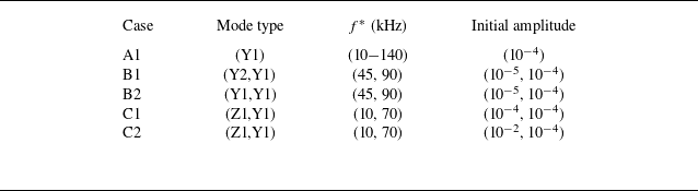
In this section, we conduct a systematic parametric study using NPSE3D to investigate the nonlinear development of vortex modes. Specifically, we aim to evaluate whether classical secondary instabilities – including fundamental, subharmonic and combination resonances, well-documented in two-dimensional boundary layers – are also active in the present three-dimensional configuration. For this purpose, three groups of test cases are designed, as detailed in table 2. Group A investigates the self-interaction of the Y1 mode, as well as the potential fundamental resonance that may arise simultaneously during the self-interaction process (Chen et al. Reference Chen, Dong, Tu, Yuan and Chen2023). Group B focuses specifically on the potential subharmonic resonance. Group C examines the detuned interactions between the Y- and Z- modes as well as the potential combination resonance with a more general frequency relationship (neither harmonic nor subharmonic). Note that the primary modes in groups A and B belong to the Y1 mode instability since it represents the most unstable mode in the present case.
Initial computational settings used in NPSE3D analysis.

(a) NPSE3D analysis of mode Y1 in a wide frequency range. The primary mode is marked as red and the nonlinear generated MFD is marked as blue. The most amplified frequency is 70 kHz, as illustrated in the figure. (b) Comparison of amplitude spectrum at
 $\mathit{X}^*= 1000$
mm obtained by LPSE3D and NPSE3D.

4.1. Fundamental interactions
In this section, we first examine the self-interaction of the disturbance. To simplify the calculation, the NPSE3D simulation includes only one primary frequency and the nonlinearly generated MFD. The NPSE3D calculations initiate at the near-neutral point of each mode, with the inlet disturbance temperature amplitude of 0.0001.
Figure 8 depicts the evolution of the Y1 mode at multiple frequencies. Under the influence of MFD, the modal amplitude exhibits a suppressed growth rate compared with the linear case, while saturation occurs at approximately the same amplitude across all frequencies. Notably, the saturation amplitude for temperature disturbances of the primary mode approaches 0.3. No significant secondary amplitude growth is observed, indicative of the absence of fundamental resonance. This behaviour contrasts sharply with findings by Chen et al. (Reference Chen, Dong, Tu, Yuan and Chen2023) in a three-dimensional attachment-line boundary layer study, where the Mack mode triggers fundamental resonance prior to nonlinear saturation, inducing rapid growth of MFD and streaky structures. Notably, the Z1 mode also exhibits a consistent saturation amplitude during the nonlinear stage. Its overall saturation process remains unchanged regardless of the initial amplitude. Additionally, the self-interaction slightly lowers the peak frequency of vortex instabilities, as shown in figure 8(b), which will be further explored in § 4.4.
4.2. Subharmonic interactions
Subharmonic resonance is one of the most efficient secondary-instability mechanisms in the low-speed regime (Herbert Reference Herbert1988; Kachanov Reference Kachanov1994), yet appears to be less prominent in hypersonic flows (Sivasubramanian & Fasel Reference Sivasubramanian and Fasel2014; Chen et al. Reference Chen, Zhu and Lee2017). To examine whether subharmonic-resonance-like interactions are active in the present 3-D configuration, we investigate the nonlinear interactions between the fundamental Y1 mode (90 kHz) and the nominally subharmonic Y1/Y2 mode (45 kHz) in cases B1 and B2. It is important to note that the choice of frequency here does not qualitatively affect the results of the subharmonic resonance discussed in this subsection.
(a,b) Maxima temperature amplitude evolution process along the streamwise direction for the interaction between the Y1 mode at 90 kHz and the subharmonic mode (45 kHz): Y2 mode for case B1 and Y1 mode for case B2. The phase velocities of the primary wave and subharmonic wave in (c) case B1 and (d) case B2, are shown by red and blue dashed lines, respectively. The growth rates of the subharmonic mode are indicated by black solid and dotted lines, with the dotted line representing the linear case.

Figure 9(a,b) reveal that both cases B1 and B2 exhibit moderate secondary growth in their subharmonic modes. The amplitude evolution features a pronounced inflection point near
 $X^*$
= 950 mm, which coincides with abrupt variations in phase velocity (as shown by the dashed lines in figure 9
c,d), thereby suggesting the occurrence of mode synchronisation.
Decomposition of the subharmonic disturbance energy budget for case B1. The density of the linear and nonlinear energy budget at
 $X^* = 1007$
mm are shown in panels (b) and (c), where the pink dashed lines represent the critical layer.

Figure 10(a) decomposes the total growth rate (
 $\sigma _{{E}}$
) into linear (
 $\sigma _{\mathcal{L}}$
) and nonlinear (
 $\sigma _{\mathcal{N}_{\textit{mfd}}}$
,
 $\sigma _{{\mathcal{N}}_{\textit{others}}}$
) components for case B1. The results of case B2 exhibit a comparable trend and are therefore omitted for brevity. Notably, the increase in the growth rate of the subharmonic mode is primarily attributed to nonlinear interactions with the primary mode, where the contribution from MFD appears to be relatively insignificant. This energy redistribution mechanism fundamentally differs from previous studies on parametric resonance, where saturated primary modes catalyse secondary instability growth (Wu, Stewart & Cowley Reference Wu, Stewart and Cowley2007; Chen et al. Reference Chen, Zhu and Lee2017). Figures 10(b) and 10(c) map the energy budget near the synchronisation location (
 $X^*$
= 1007 mm), showing that
 $\sigma _{\mathcal{L}}$
and
 $\sigma _{\mathcal{N}}$
exhibit spatially anti-correlated distributions: regions of positive linear contribution density correspond spatially to negative nonlinear contribution density.
4.3. Detuned interactions
Variations in the maximum temperature disturbance along the streamwise direction of the Z1–Y1 mode interaction dominated by the (a) Y1 mode (case C1) and (b) Z1 mode (case C2), where the dashed lines represent the results of the self-interaction case.

An intriguing detuned interaction occurs between a high-frequency Y1 mode and a low-frequency Z1 mode. Such interactions may drive multi-scale turbulence generation due to pronounced spatio-temporal disparities between modal frequency spectra and spatial structures. To probe this mechanism, we examine the representative Y1 (70 kHz, outer) and Z1 (10 kHz, inner) mode interaction, as shown in figure 11. Specifically, two scenarios were considered by selectively prescribing the dominant mode. When the Y1 mode dominates (figure 11 a), the Z1 mode evolves similarly to its self-interaction case, suggesting minimal cross-impact before the calculation fails to converge. Conversely, when the Z1 mode dominates (figure 11 b), the growth rate of the Y-mode is reduced.
Evolution process of streamwise velocity perturbations of the (a) difference mode, (b) sum mode, (c) MFD, (d) Y1 mode and (e) Z1 mode under the Z1 mode dominant condition. The shape functions are normalised at each streamwise station. The yellow isosurface and the purple isosurface represent negative and positive velocity disturbance at 0.5.

Figure 12 illustrates the evolution of the streamwise velocity disturbance shape function under the dominant influence of the Z1 mode. Throughout the streamwise evolution, the distribution of both the Y1 mode (figure 12 d) and Z1 mode (figure 12 e) remain nearly unchanged and can be distinctly identified by two separate base velocity isosurfaces. For both difference and sum modes, their shape functions concentrate near the critical layer of the Y1 mode. It can be observed that the MFD gradually shifts from the root region of the streamwise vortex towards the shoulder region, which will predictably lead to nonlinear interactions with the Y-mode located at the shoulder. Subsequent analysis (§ 4.4) will show that the MFD plays a dominant role in suppressing the Y1 mode.
4.4. Role of MFD
Prior analyses of nonlinear streamwise vortex interactions reveal that MFD plays a pivotal role in disturbance saturation. As demonstrated in figure 8, MFD drives disturbances towards uniform saturation amplitudes across all frequencies during nonlinear evolution and concurrently shifts the spectral peak (linear regime) to a lower frequency band. To elucidate this critical mechanism, the present section investigates how MFD reconstructs the base flow shear distribution and subsequently modulates modal disturbance evolution.
(a) Energy budget of the most unstable Y1 mode at 70 kHz along the streamwise direction for the linear (dashed lines) and nonlinear (solid lines) cases. (b) Direct nonlinear energy transfer from MFD (
 $\sigma _{\mathcal{N}_{\textit{mfd}}}$
) and linear energy transfer implicitly caused by MFD via modifying the shape function (
 $\sigma _{\mathcal{L}} - \sigma _{\textit{Linear}}$
) to the Y1 mode.

Comparison of the base flow and the shape function of the primary mode at 70 kHz at
 $\mathit{X}^* =$
1000 mm in the (a) linear and (b) nonlinear cases. The white dashed lines denote the non-dimensional base flow
 $\bar {u} = 0.1:0.1:0.8$
. The coloured contour is referred to as the shear magnitude of the streamwise velocity
 $\bar {u}_s$
. The red dashed contour denotes the streamwise velocity magnitude, namely
 $|\hat u|$
, of the primary disturbance.

4.4.1. Energy transfer analysis
Figure 13(a) shows the streamwise evolution of the energy budget for the 70 kHz Y1 mode in the self-interaction case A1. As expected, wall-normal production (
 $P_y$
) dominates throughout. The MFD significantly modifies production terms through dual mechanisms: direct nonlinear energy transfer (
 $\sigma _{\mathcal{N}_{\textit{mfd}}}$
) and indirect shape function modification (
 $\sigma _{\mathcal{L}} - \sigma _{\textit{Linear}}$
). The former always exerts a damping effect, while the latter initially enhance the energy transfer from the base flow and then eventually causes the disturbance to lose energy, as displayed in figure 13(b). Similar energy characteristics also occur in Z1 modes. Figure 14 unveils how MFD affects the disturbance by distorting the vortex profile. The shear magnitude of the streamwise velocity
 $\bar {u}_s$
(Zhang et al. Reference Zhang, Dong, Liu, Yuan, Chen and Chen2022) is defined as
 \begin{align} \bar {u}_s = \left [\left (\partial ({\bar {u}+u_{\textit{mfd}}})/\partial \mathit{Z}\right )^2 + \left (\partial ({\bar {u}+u_{\textit{mfd}}})/\partial \mathit{Y}\right )^2\right ]^{1/2}. \end{align}
The MFD eliminates the high-shear layer at the vortex shoulder where the linearly unstable primary mode resides, thereby forcing the shape function to diffuse upward.
MFD structure generated by the 70 kHz Y1 mode is presented, along with profiles at four stations. In these profiles, red and blue denote the high-speed and low-speed streaks, respectively. The increase in the wall friction coefficient caused by MFD is also illustrated.

Figure 15 presents the spatial structure of the MFD and the corresponding modifications in the skin friction coefficient relative to the base flow. The MFD consists of high- and low-speed streaks (HSS and LSS) near the high-shear layers of the base flow. Before
 $\mathit{X}^* = 980$
mm, the HSS and LSS are constricted side by side atop of the streamwise vortex. Simultaneously, the distortion’s shape function starts to expand, locally reducing the shear strength of the base flow, as shown in figure 14. Subsequently, the LSS stretches to the vortex’s top, creating a substantial low-speed region. Finally, at
 $\mathit{X}^* = 1082$
mm, the HSS expands towards the wall, increasing the friction coefficient.
(a) Energy budget of the 70 kHz disturbance in the case dominated by the Z1 mode (case C2). (b) Energy budget density owing to the MFD at
 $X^* = 935$
mm. Here, the red and blue contour lines indicate values of +0.01 and −0.01, respectively.

(a) Maxima amplitude of the Y1 mode sensitivity profile to base distortion, namely
 $\bigtriangledown _{Q}\alpha$
, at
 $X^*$
= 960 mm. (b–f) Real parts of the density of the sensitivity profile at 120 kHz. The pink dashed line indicates
 $99\,\%$
of the perturbation energy as defined by (2.5), serving as the reference for the modal distribution.

For case C1, the Y1 mode was significantly less amplified during the Z1 mode’s saturation phase. To determine the underlying mechanism, we conducted an energy transfer analysis (figure 16
a), which reveals that MFD dominates energy redistribution over other nonlinear interactions. Specifically, the spatial distribution of the MFD energy budget density at
 $X^*$
= 935 mm (figure 16
b) shows that although the Y1 mode amplitude remains sub-saturated, MFD shifts to the streamwise vortex shoulder, directly overlapping the Y1 mode’s region. The high- and low-speed streaks on the vortex shoulder exhibit distribution patterns similar to the self-interaction Y1 mode case.
4.4.2. Sensitivity analysis
In the preceding analysis, the MFD significantly influences the energy budget of disturbances, driving nonlinear outcomes that deviate markedly from linear predictions. Notably, the dominant mode in the nonlinear analysis shifts to a lower frequency. This motivates our exploration of the influence of MFD on mode evolution and interaction. To the best of the authors’ knowledge, this is the first study that addresses the sensitivity of streamwise vortex modes.
Figure 17 displays the frequency-dependent sensitivity amplitude of the Y1 mode to different base flow components. Given the small streamwise variation in sensitivity, results are shown exclusively at a representative station
 $X^* =$
960 mm. It reveals that all sensitivity components increase rapidly with frequency, demonstrating that higher-frequency modes are more sensitive to base flow distortion – a finding consistent with enhanced MFD effects at higher frequencies (see reduced peak frequency in figure 8). Notably, velocity-component sensitivities exceed temperature/pressure sensitivities by orders of magnitude, indicating that base velocity distortions dominate stability modifications. This velocity-dominant trend aligns with observations from Park & Zaki (Reference Park and Zaki2019) for a flat-plate boundary layer. Furthermore, normalised sensitivity density distributions at one representative frequency (140 kHz), coinciding with the mode shape region, concentrate exclusively on the wall-normal high-shear layer, highlighting the important role of the latter. Since the streamwise velocity component are substantially stronger than other velocity components in MFD, subsequent analysis focuses solely on its impact on modal stability.
(a) Modified modal growth rate and (b) modified phase velocity at
 $X^* = 960$
mm under the distortion of streamwise base velocity
 $\delta U$
. The distortion profile is abstracted from the baseline case (refer to figure 15). Red dots denote the growth rate of the original mode, blue dots illustrate the effect of the distortion itself, blue dots indicate the contribution from the change in base-flow shear and the black dots represent their combined effect.

Spatial distribution of the streamwise velocity sensitivity at
 $X^*$
= 960 mm, showing the real and imaginary parts of the streamwise velocity component for the (a,b) direct mode and (c,d) adjoint mode, as indicated by the circle in figure 18. The real and imaginary parts of the density of the streamwise velocity sensitivity are respectively illustrated in panels (e–h) and (i–l).

The MFD’s influence is quantified by multiplying its profile with the sensitivity function. Both the streamwise velocity (
 $U$
) and its spatial derivatives (
 $\partial U / \partial l$
) were evaluated using distortion profiles from the baseline case (figure 15). Interestingly, these components exhibit opposing effects: while modification of base flow derivatives (
 $\partial U_{\textit{mfd}} / \partial l$
) weaken modal growth as well as the phase velocity, the base flow velocity distortion (
 $U_{\textit{mfd}}$
) itself strengthens them, with the former being dominant, as shown in figure 18.
Following the work of Park & Zaki (Reference Park and Zaki2019), we further decompose the sensitivity to the streamwise velocity into four components, specifically
 $\hat {\boldsymbol{S}}_{U}=\hat {\boldsymbol{S}}_{U}^1+\hat {\boldsymbol{S}}_{U}^2+\hat {\boldsymbol{S}}_{U}^3+\hat {\boldsymbol{S}}_{U}^4$
, which correspond to the shear of the streamwise velocity, the convective term of the flow, the dissipation caused by viscosity, and the remaining terms associated with temperature and pressure, respectively. The forms of these components are given in Appendix A.
Figure 19 illustrates the spatial distribution characteristics of the streamwise velocity sensitivity at the
 $X^*$
= 960 mm station. It is evident that the shape functions exhibit a typical wave packet structure in the
 $\eta$
–
 $\zeta$
plane. The real and imaginary parts display a phase difference of approximately
 $\pi /2$
. As shown in panels (e–h), all the components exhibit a multi-pole distribution near the critical layer. The spatial distribution of the real part of the sensitivity reflects the characteristics of the modal phase velocity sensitivity to the base flow. The sensitivities to velocity shear (
 $\hat {S}^{1}_{U}$
) and those associated with temperature and pressure terms (
 $\hat {S}^{4}_{U}$
) exhibit remarkably similar structures: both display positive values above and negative values below in the vicinity of the critical layer. Sensitivity distributions related to convective terms and viscous terms (
 $\hat {S}^{2}_{U}$
,
 $\hat {S}^{3}_{U}$
) are predominantly positive near the critical layer. The imaginary part of the sensitivity directly reflects the negative variation in the modal growth rate, exhibiting a positive–negative distribution around the critical layer.
Histogram of the (a) growth rate and (b) phase velocity distortions of the Y1 mode at
 $X^* =$
960 mm, which is illustrated by the circle in figure 18, when the flow is distorted by
 $U_{\textit{mfd}}$
in the baseline case. The black columns represent the total distortion
 $\delta \alpha _i$
and
 $\delta c_{\textit{ref}}$
in panels (a) and (b), respectively. Each total distortion is divided into four parts.

Figure 20 compares the contribution of the different sensitivity components to the variations of the growth rate and phase velocity at the same place. As depicted in figure 20(a), the bar chart for the growth rate contribution (
 $-\alpha _i$
) reveals that the shear of the base flow field
 $\hat{\mathcal{S}}^1_U$
predominantly governs the influence of MFD on modal stability, followed by the convective component
 $\hat{\mathcal{S}}^2_U$
, and the temperature and pressure component
 $\hat{\mathcal{S}}^4_U$
. While
 $\hat{\mathcal{S}}^1_U$
and
 $\hat{\mathcal{S}}^4_U$
show a stabilising effect,
 $\hat{\mathcal{S}}^2_U$
exhibits a destabilising effect. The viscous component
 $\hat{\mathcal{S}}^3_U$
exhibits negligible impact on the mode. For the phase velocity in figure 20(b), the streamwise velocity shear component
 $\hat{\mathcal{S}}^1_U$
constitutes the primary positive contribution, whereas the convection and temperature-pressure terms
 $\hat{\mathcal{S}}^2_U$
and
 $\hat{\mathcal{S}}^4_U$
both display negative effects, and the contribution value of the viscous component
 $\hat{\mathcal{S}}^3_U$
remains nearly zero. In conclusion, modal instability is most sensitive to the change of the base flow shear. It is worth noting that although MFD generated during the evolution of modal disturbances varies slightly depending on the frequency, for modes belonging to the same branch, the results are qualitatively consistent.
5. Vortex breakdown simulations
The NPSE3D method demonstrates its capability to effectively capture the characteristics of streamwise vortex mode development in the early stages of disturbance evolution. However, as nonlinear interactions become increasingly significant in the later stages, substantial changes in the streamwise wavenumber and disturbance shape function arise, violating the assumption inherent to the parabolised formulation. To resolve this limitation and also verify the computational results of the NPSE3D, we perform DNS to analyse the breakdown mechanisms of shoulder vortices in the late transition stage. To achieve high-fidelity results while optimising computational resources, the mesh is significantly refined in the azimuthal angle range
 $\theta = 45^{\circ }$
–
 $60^{\circ }$
(
 $\Delta \theta = 0.10^\circ$
), where the shoulder streamwise vortex resides. The grid for simulating the transition condition is interpolated from the basic flow grid and truncated in the streamwise direction from
 $X^*$
= 600 to 1400 mm, with the sponge zone lying between
 $X^*$
= 1300 and 1400 mm. The grid contains 1980 points in the streamwise direction, 369 points in the lateral direction and 251 points in the wall-normal direction. The grid resolution is
 $\triangle x^{+}_{\textit{max}} \times \triangle y^{+}_{\textit{min}} \times \triangle z^{+}_{\textit{max}} = 20\times 0.5\times 20$
. As per the research by Chen et al. (Reference Chen, Dong, Tu, Yuan and Chen2022), the current simulation can be regarded as QDNS (with grid resolution lying between that of large eddy simulation and that of DNS). As shown in Appendix B,
 $\triangle x^{+}_{\textit{max}}$
and
 $ \triangle z^{+}_{\textit{max}}$
remain consistently around 10 for the region on which we focus (
 $X^* \lt$
1200 mm), which is sufficient for our purpose.
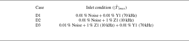
At the inlet boundary conditions, modal profiles incorporating each Z1 and Y1 modes or both were imposed, along with random noise constituting 0.01 % of the incoming flow. The impact of these random noise amplitude on the modal evolution process was evaluated and found to be negligible. The numerical simulation parameters are listed in table 3.
Simulation cases.

Visualisation of the instantaneous flow field structure using the Q criterion (Q = 0.0004 for DNS and 0.0001 for NPSE3D/LPSE3D), with isosurfaces coloured by the time-averaged and base streamwise velocity. Local enlarged views of the vortex structures at selected stations are presented for (a) DNS, (b) NPSE3D and (c) LPSE3D.

Figure 21 compares Q-criterion isosurfaces from DNS, NPSE3D and LPSE3D simulations during transition onset (case D1). The results demonstrate that NPSE3D successfully reproduces the key features of the DNS flow structures. The stretch of secondary vortex-leg connecting to the primary vortex (as highlighted in figure 21) is reminiscent of the ‘finger vortices’ reported by Chen et al. (Reference Chen, Dong, Chen, Yuan and Xu2021) during stationary cross-flow breakdown at Mach 6. Specifically, the upstream hairpin vortex splits downstream, presumably due to vortex reconnection (Yao & Hussain Reference Yao and Hussain2022) between primary hairpins and MFD-induced streamwise vortices, as sketched by figure 22. Notably, the splitting of such vortex structures has also been observed during the transition process of cross-flow vortices on swept wings and Görtler vortices during their late-stage transition stage (Bonfigli & Kloker Reference Bonfigli and Kloker2007; Casacuberta et al. Reference Casacuberta, Groot, Hickel and Kotsonis2022; Brockhaus et al. Reference Brockhaus, Sescu, Es-Sahli and Hattori2024), as well as of streaky structures downstream a randomly distributed roughness patch (Wang et al. Reference Wang, Chen, Tu, Wan and Chen2024).
(a) Schematic vortex topology: (i) MFD and (ii) base flow superimposed with the Y1 mode from NPSE3D. Structures are visualised by the Q = 0.0005 isosurface coloured by streamwise vorticity (red, positive; blue, negative). (b) Cartoon of the splitting process: the MFD and primary mode can be viewed as thread and bridge, respectively.

Figure 23 illustrates the evolution characteristics of disturbances in case D1 at three representative stations. At the streamwise station of
 $X^*$
= 900 mm, the disturbance remains in its linear growth phase, with the root mean square (rms) distribution featuring Y1 mode distribution. Further downstream at
 $X^*$
= 1000 mm, the MFD amplitude gradually accumulates and significantly influences the local flow profile. Through energy analysis, as detailed in the previous section, it is evident that the MFD primarily modulates the growth of the modal disturbance by diminishing the dominant source term associated with the local velocity gradient, thereby inducing a saturation state for the perturbation. Meanwhile, the disturbance progressively expands to encompass the entire wall-normal shear layer region with its peak moving towards the upper left corner of the shear layer. This observation qualitatively aligns with the NPSE3D results simulating the self-interaction of a single Y1 mode (refers to figure 14). Further downstream to
 $X^*$
= 1100 mm, as the flow field undergoes deformation, the disturbance evolution enters the downwash region associated with the streamwise vortex. A significant peak emerges in this region, displaying morphological similarities to the instability process of cross-flow vortices at their downwash region (Xu et al. Reference Xu, Chen, Liu, Dong and Fu2019). However, no comparable unstable mode characteristics are identified in the multi-dimensional stability analysis of the upstream streamwise vortex, suggesting that this disturbance arises from nonlinear interactions rather than inherent linear mechanisms. Figure 23(d) compares the perturbation amplitudes from DNS and NPSE3D, showing a good agreement between the two approaches.
Spatial distribution of the root mean square (rms) of temperature fluctuations of case D1 at
 $X^*$
= (a) 900 mm, (b) 1000 mm and (c) 1100 mm, as obtained from DNS. The amplitude of disturbance at 70 kHz in DNS is compared with NPSE3D in panel (d).

MFD, flow field visualised via Q-criterion (Q = 0.0004), wall friction of the instantaneous flow field and the time-averaged wall friction elevated relative to the base flow for the Y1 mode case at the late stage. Additionally, the flow field marked by rectangular boxes is included to illustrate the vortex structures associated with wall friction lift-up, coloured by streamwise velocity and vorticity in the Z-direction, as well as the vortex structures in the flow field at a later stage.

To achieve a better comprehension of the transition process, figure 24 illustrates several critical features of the flow field during the late saturation stage of the disturbance. These include the visualisation of vortex structures using the Q criterion, the spatial distribution of the instantaneous wall friction coefficient and the rise of the mean flow wall friction coefficient relative to the base flow. Notably, the spatial evolution of the MFD is very reminiscent of the NPSE3D results (refer to figure 15). Upon reaching the saturation stage, the Y1 mode induces a typical hairpin vortex structure in the shoulder region of the streamwise vortex. As the flow evolves downstream, these vortex structures migrate towards the wall along the downwash region of the vortex. The square-marked regions in the figure highlight specific locations where the wall friction coefficient increases, with the vorticity distribution in the Z-direction (depicted by red for clockwise rotation and blue for counterclockwise rotation) offering a more intuitive visualisation of the vortex dynamics. When the shape function of the Y1 mode fully encompasses the shoulder region of the streamwise vortex, it gradually transforms from a hairpin to a horseshoe configuration. During this transformation, the right leg of the horseshoe vortex generates a counter-rotating vortex roll near the wall, significantly influencing the local wall friction coefficient. Simultaneously, the disturbance near the wall triggers an HSS, ultimately leading to adjustments in the shear layer within the streamwise vortex and resulting in an increase of the time-averaged wall friction. As the horseshoe vortex evolves downstream, its right leg is stretched due to wall drag, eventually forming a streamwise-extended structure. Concurrently, the roll atop the horseshoe vortex breaks down under the influence of the MFD, cascading into a series of vortex clusters. This process catalyses the breakdown of the streamwise vortex.
(a) Results of wall friction rise at
 $\theta ^\circ = 53^\circ$
, which is illustrated in panels (b–d) as the white dashed line, for the Y1 mode (red solid line), Z1 mode (blue solid line) and interaction case (black solid line), together with the laminar state and the turbulence estimate (van Driest Reference van Driest1951) as a reference. (b–d) Time-averaged wall friction in the three cases, where the purple dashed contour lines indicate overshoot areas.

Figure 25(a) reveals wall friction evolution at
 $\theta =53^\circ$
for cases D1–D3, showing that transition onset (marked by friction rise) aligns temporally regardless of the dominant mode. During late transition stages (figure 25
b–d), all cases exhibit friction overshoot – notably, Z1 mode induces earlier overshoot due to their proximity to the wall, where MFD directly modifies near-wall profiles. Additionally, the mode-interaction case (D3) exhibits an advanced overshoot location compared with Y1 or Z1 mode-only cases. This acceleration mechanism is corroborated by the Q-criterion at friction-rise onset (
 $X^* \approx 1050$
mm, refer to figure 26). While Z1 mode generates persistent near-wall large-scale structures, mode interactions dissipate these features rapidly. Collectively, these findings demonstrate that modal interactions accelerate disturbance saturation and structural breakdown, thereby hastening transition. Moreover, the friction coefficient peak in interaction cases exceeds single-mode cases, presumably due to MFD amplification through multi-modal interactions.
Flow field structures at the wall friction lift-up positions for the (a) Y1 mode dominant (case D1), (b) Z1 mode dominant (case D2) and (c) interaction (case D3) cases at Q = 0.0004.

Finally, we examine the disturbance spectra within the near-wall region to elucidate the transition mechanisms. Figure 27 depicts the spatial distribution of temperature disturbances in the streamwise and frequency domains for the three cases. For the Y1 mode case, the dominant frequency of 70 kHz and its first harmonic (140 kHz) are distinguishable. Furthermore, during the initial stages of transition at approximately
 $X^*$
= 1050 mm, a broad peak centred around 35 kHz is observed. This finding aligns with subharmonic growth documented in § 4.2, suggesting that subharmonic instability mechanisms also play a significant role. For the Z1 mode case, disturbances exhibit substantial amplitudes in the upstream region, resulting in a faster growth rate of low-frequency components compared with the Y1 mode scenario. Additionally, the prominence of disturbance peaks within the 60–100 kHz frequency range underscores the notable contribution of Y1 mode instabilities during Z1 mode dominant transitions. In the interaction case, the spectral features become more complex, showing the coexistence of both Z1 and Y1 modes, their harmonics, as well as difference and sum frequencies generated by their interactions. Furthermore, higher-order harmonics are excited through interactions between these modes. As previously demonstrated through energy analysis, disturbances primarily extract energy from the shear in the flow field. The nonlinear effects accelerate the process of energy extraction by disturbances from the base flow, thereby enhancing the magnitude of overshoot.
Near-wall disturbance spectra for cases with (a) Y1 mode dominant (case D1), (b) Z1 mode dominant (case D2) and (c) mode interaction (case D3). Comparative results of the disturbance spectra for the three cases at streamwise locations of (d)
 $X^*$
= 1000 mm, (e)
 $X^*$
= 1100 mm and (f)
 $X^*$
= 1125 mm.

6. Conclusions
This study investigates the nonlinear stability and transition mechanisms of streamwise vortices over the HyTRV lifting body by employing both linear and nonlinear multi-dimensional stability analysis methods (BiGlobal, LPSE3D, NPSE3D) alongside direct numerical simulation (DNS). Linear modal analysis identifies two primary instabilities: the Y-mode located at the vortex top, which exhibits broader frequency ranges, higher amplification rates and higher phase velocities compared with the Z-mode situated at the vortex root. Energy budget decomposition reveals distinct energy production, with Y-modes predominantly sustained by wall-normal shear production (
 $P_y$
) and Z-mode mostly depending on lateral shear production (
 $P_z$
). While the cross-flow vortices and Görtler vortices arise from primary instabilities of the boundary layer, the streamwise vortices in the present study are the base flow itself and emerge from the convergence of the fluid. Therefore, the primary instabilities of the streamwise vortices in the present study are analogous to the secondary instabilities of the cross-flow and Görtler vortices.
The nonlinear self-interactions of the Y-mode yield amplitude saturation without triggering the fundamental resonance, in stark contrast with the attachment-line boundary layer where the primary mode is prone to strong fundamental resonance (Chen et al. Reference Chen, Dong, Tu, Yuan and Chen2023). Detuned interaction between high-frequency Y-mode and low-frequency Z-mode is also found to be weak in the weakly nonlinear stage. By comparison, moderately strong subharmonic resonance is observed.
Mean flow distortion (MFD) plays a pivotal role in nonlinear development of vortex modes. It weakens the shear layer notably, thereby causing the saturation of the primary mode. Moreover, MFD manifests as longitudinal vortical structures with alternating positive and negative streamwise vortices, which can interact with the primary mode exhibiting a hairpin vortex. By vortex reconnection, the primary hairpin vortex splits into two hairpin vortices. This splitting process continues, resulting in hairpin wave-packet.
Sensitivity analysis further demonstrates that velocity components within base-flow distortions exert the strongest influence on stability modifications, with orders-of-magnitude higher sensitivity than temperature/pressure variations. Higher-frequency modes exhibit significantly greater susceptibility to these sensitivity effects.
DNS results are in good agreement with NPSE3D results up to the weakly nonlinear stage, and show details about the breakdowns process during which subharmonic disturbances emerge and become pronounced. Seeding both the Y-mode and the Z-mode turns out to precipitate the transition process.
Although only a specific configuration is considered, the nonlinear stability analyses developed in this work can be straightforwardly applied to other flows featuring streamwise vortical structures. The close similarity regarding the development of vortical structures during the breakdown process in apparently different flows (e.g. Casacuberta et al. Reference Casacuberta, Groot, Hickel and Kotsonis2022; Wang et al. Reference Wang, Chen, Tu, Wan and Chen2024) implies the universal vortex-splitting mechanism which warrants further studies.
Acknowledgements
The authors acknowledge the fruitful suggestions from Dr G. Tu, Dr B. Wan, Dr S. Dong and Dr S. Liu.
Funding
This study is supported by National Natural Science Foundation of China (grant nos. 12372225 and 12272395) and the National Numerical Wind-tunnel Project (NNW).
Declaration of interests
The authors report no conflict of interest.
Appendix A. Detailed expressions of the sensitivity to streamwise velocity
In this section, we present detailed expressions of the sensitivity of the complex streamwise wavenumber to streamwise base-flow velocity distortions, namely
 $\hat {\boldsymbol{S}}_{U}=\hat {\boldsymbol{S}}_{U}^1+\hat {\boldsymbol{S}}_{U}^2+\hat {\boldsymbol{S}}_{U}^3+\hat {\boldsymbol{S}}_{U}^4$
, where the overall component is derived based on the BiGlobal stability analysis matrix presented by Chen et al. (Reference Chen, Dong, Tu, Yuan and Chen2022).
The first term originates from the shear components of the base flow in the streamwise velocity, primarily involving the terms
 $\partial U/\partial y$
and
 $\partial U/\partial z$
,
 \begin{align} \widehat {\boldsymbol{S}}_U^1 &= \frac {\partial \rho \widehat {u}^{\dagger *} \widehat {v}}{\partial y} + \frac {\partial \rho \widehat {u}^{\dagger *} \widehat {w}}{\partial z}. \end{align}
Note that in this appendix, the superscript
 $^*$
denotes the complex conjugate part and the over-bar of the base-flow quantities has been omitted for simplicity. The second term arises from the non-parallel effects of the perturbations, incorporating the spatial derivatives of the streamwise velocity perturbations with respect to the base flow,
 \begin{align} \widehat {\boldsymbol{S}}_U^2 &= \alpha \left [ -i\rho \big ( \widehat {u}^{\dagger *} \widehat {u} + \widehat {v}^{\dagger *} \widehat {v} + \widehat {w}^{\dagger *} \widehat {w} \big ) + i\gamma M^2 \widehat {p}^{\dagger *} \widehat {p} - i \operatorname {Pr} \rho \widehat {T}^{\dagger *} \widehat {T} \right ] \\\nonumber &\quad - i\rho \widehat {u}^{\dagger *} \frac {\partial \widehat {u}}{\partial x} + \frac {\rho }{T} U_x \widehat {u}^{\dagger *} \widehat {T} - \frac {\partial \left ( \widehat {u}^{\dagger *} \widehat {T} \rho V / T \right )}{\partial y} - \frac {\partial \left ( \widehat {u}^{\dagger *} \widehat {T} \rho W / T \right )}{\partial z} \\\nonumber &\quad - \rho \widehat {v}^{\dagger *} \widehat {v}_x + \frac {\rho }{T} V_x \widehat {v}^{\dagger *} \widehat {T} + \operatorname {Pr} \rho \frac {T_x}{T} \widehat {T}^{\dagger *} \widehat {T} - \operatorname {Pr} \rho \widehat {T}^{\dagger *} \widehat {T}_x + \frac {\rho }{T} W_x \widehat {w}^{\dagger *} \widehat {T} - \rho \widehat {w}^{\dagger *} \widehat {w}_x . \end{align}
The third term represents a combination of terms directly associated with viscous dissipation,
 \begin{align} \widehat {\boldsymbol{S}}_U^3 &= -i \frac {\alpha }{R} \left [ \frac {\partial \left ( \mu \mu _m \widehat {v}^{\dagger *} \widehat {T} \right )}{\partial y} + \frac {\partial \left ( \mu \mu _m \widehat {w}^{\dagger *} \widehat {T} \right )}{\partial z} - 2G \frac {\partial \left ( \mu \widehat {T}^{\dagger *} \widehat {v} \right )}{\partial y} - 2G \frac {\partial \left ( \mu \widehat {T}^{\dagger *} \widehat {w} \right )}{\partial z} \right ] + \nonumber\\\nonumber & \quad \frac {1}{R} \left [ -\frac {\partial \left ( \widehat {u}^{\dagger *} \widehat {T}_y \mu \mu _m \right )}{\partial y} - \frac {\partial \left ( \widehat {u}^{\dagger *} \widehat {T}_z \mu \mu _m \right )}{\partial z} + \frac {\partial ^2 \left ( \mu \mu _m \widehat {u}^{\dagger *} \widehat {T} \right )}{\partial y^2} + \frac {\partial ^2 \left ( \mu \mu _m \widehat {u}^{\dagger *} \widehat {T} \right )}{\partial z^2} \right . \\\nonumber &\quad \left . - \frac {\partial \! \left ( \widehat {u}^{\dagger *} \widehat {T} T_y \mu \mu _{mm} \right )}{\partial y} - \frac {\partial \! \left ( \widehat {u}^{\dagger *} \widehat {T} T_z \mu \mu _{mm} \right )}{\partial z} + \frac {\partial \! \left ( \widehat {v}^{\dagger *} \widehat {T} T_x \mu \mu _{mm} l_0 \right )}{\partial y} + \frac {\partial \! \left ( \widehat {v}^{\dagger *} \widehat {T}_x \mu \mu _m \right )}{\partial y} \right . \\\nonumber &\quad \left . + 2G \frac {\partial \left ( \widehat {T}^{\dagger *} \widehat {T} T_x \mu \mu _{mm} U_y \right )}{\partial y} + 2G \frac {\partial \left ( \widehat {T}^{\dagger *} \widehat {T} T_x \mu \mu _{mm} U_z \right )}{\partial z} + \frac {\partial \left ( \mu \mu _{mm} T_x \widehat {w}^{\dagger *} \widehat {T} \right )}{\partial z} \right . \\\nonumber &\quad \left . + \frac {\partial \left ( \mu \mu _m \widehat {w}^{\dagger *} \widehat {T}_x \right )}{\partial z} + 2G \frac {\partial \left ( \mu \widehat {T}^{\dagger *} \widehat {u}_y \right )}{\partial y} + 2 G \frac {\partial \left (\mu \widehat {T}^{\dagger *} \widehat {u}_z\right )}{\partial z}+2 G \frac {\partial \left (\mu \widehat {T}^{\dagger *} \widehat {u}_x\right )}{\partial y}+ \right . \\&\quad \left . 2G \frac {\partial \mu \widehat {T}^{\dagger *} \widehat {w}_x}{\partial z} \right ] . \end{align}
The fourth term consolidates all contributions involving the temperature and pressure perturbation components,
 \begin{align} \widehat {\boldsymbol{S}}_U^4 &= \alpha \big [ -i\rho \widehat {p}^{\dagger *} \widehat {T} + iG \widehat {T}^{\dagger *} \widehat {p} \big ] - \frac {\gamma Ma^2_\infty }{T} U_x \widehat {u}^{\dagger *} \widehat {p} - \gamma Ma^2_\infty \frac {\partial \left ( V \widehat {u}^{\dagger *} \widehat {p} / T \right )}{\partial y} \\\nonumber &\quad - \gamma Ma^2_\infty \frac {\partial \left ( W \widehat {u}^{\dagger *} \widehat {p} / T \right )}{\partial z} - \gamma Ma^2_\infty \frac {V_x}{T} \widehat {v}^{\dagger *} \widehat {p} - \gamma Ma^2_\infty \frac {T_x}{T} \widehat {p}^{\dagger *} \widehat {p} + \gamma Ma^2_\infty \widehat {p}^{\dagger *} \widehat {p}_x \\\nonumber &\quad + \left ( 2 \frac {P_0 T_x - P_x T}{T^2} \right ) \widehat {p}^{\dagger *} \widehat {T} - \rho \widehat {p}^{\dagger *} \widehat {p}_x - \gamma Ma^2_\infty \operatorname {Pr} \frac {T_x}{T} \widehat {T}^{\dagger *} \widehat {p} + G \widehat {T}^{\dagger *} \widehat {p}_x \\\nonumber &\quad - \gamma Ma^2_\infty \frac {W_x}{T} \widehat {w}^{\dagger *} \widehat {p}. \end{align}
The terms
 $G = Pr(\gamma -1)Ma^2_\infty$
,
 $\mu _m=({\rm d}\mu /{\rm d}T)/\mu$
and
 $\mu_{mm} = ({\rm d}^2\mu/{\rm d}^2T)/\mu$
are abbreviated for brevity.
Appendix B. DNS resolution
Four sets of grids were employed to assess the independence of the baseflow with respect to streamwise, azimuthal and wall-normal resolutions, namely (641
 $\times$
741
 $\times$
301), (521
 $\times$
741
 $\times$
301), (521
 $\times$
891
 $\times$
251) and (521
 $\times$
741
 $\times$
251, baseline), as shown in figure 28. There are approximately 150 points within the boundary layer in the shoulder vortex region for the baseline grid adopted in the manuscript. Evidently, further increasing the grid points in either the streamwise, the azimuthal or the wall-normal direction compared with the baseline case barely changes the base flow, thereby verifying the grid convergence.
Grid convergence analysis of the baseline flow at
 $X^*$
= 800 mm.

(a) Flow field structure in the later stages of the disturbance dominated by the Y1 mode, and (b–d) sizing of the mesh in a local wall unit.

Figure 29 illustrates the distribution of near-wall mesh discretisations accuracy across most of the surface area in the shoulder vortex region. Apart from the loss of resolution due to disturbances evolving near the wall, the dimensionless wall distances
 $\triangle x^+$
and
 $\triangle z^+$
are maintained below 10. For the dominant Y1 mode (70 kHz) and its harmonic (140 kHz), approximately 25 and 15 grid points are used per wavelength for resolution, respectively. The spatial resolution of this mesh system is comparable to that of previous study using also QDNS to analyse the vortical structures (Chen et al. Reference Chen, Dong, Tu, Yuan and Chen2022), thereby satisfying the accuracy requirements for this research.