

1 WHAT HAPPENED TO BASEMAPS IN PERCEPTUAL DIALECTOLOGY?
In Perceptual Dialectology (PD), we routinely talk about the results our basemaps bring without ever discussing the decisions that went into building the basemaps. We at least intuitively understand that a US basemap with state lines is different than one with just state capitals. Preston (Reference Preston1989) in his seminal publication laid the foundations for modern PD by making an observation that the respondents are not able to escape the influence of the details on basemaps, especially if they resemble lines. “Perhaps a map with major rivers, cities, and mountains would have prevented this sort of response” (Preston Reference Preston1989:25). We can see that even in the early work in perceptual dialectology basemaps were important, and the relation between the type of details on the basemaps and the resulting shape of perceptions was acknowledged.
However, the recognition of basemaps’ importance didn’t trigger research investigating this influence of basemap type on the results. Just the opposite happened. Preston, in his early but extremely influential research, attempted a very basic test of different basemaps, and describes his experience in the following manner:
Exactly what detail the fieldwork map for such a task should contain is difficult to determine. In a trial run using a blank outline map of the entire country, a number of respondents agreed they could not perform the task. The difficulty in determining the proper amount of detail may be further complicated by the general social and educational characteristics of the respondents. (1989:25)
The assertions above made by Preston influenced the next few decades of PD in a tremendous way. For one, the empty map never gained recognition as a valid basemap, although other approaches presented below will show that an empty basemap is useful in PD. Moreover, the attitude that nothing can be done about determining the types of details on basemaps prevailed in PD until recently when a handful of researchers and the author of the current article, devised a way to investigate the relationship between the types of basemaps and the shape of perceptions. Therefore, the attitude presented by Preston and cultivated in the field for the next decades that: “There is little that can be done to improve the instrument which elicits a hand-drawn map” (1989:125) has to be reconsidered.
Such reconsideration has not happened in the past few decades in PD. Instead, the basemap with state lines became almost a standard instrument in the field (Preston, Reference Preston1989; Benson, Reference Benson2003; Fridland, Bartlett, & Kreuz, Reference Fridland, Bartlett and Kreuz2005; Fridland & Bartlett, Reference Fridland and Bartlett2006; Bucholtz et al., Reference Bucholtz, Bermundez, Fung, Edwards and Vargas2007; Bucholtz et al., Reference Bucholtz, Bermundez, Fung, Vargas and Edwards2008). Although some of the researchers pick different types of basemaps, such as a national map with major cities indicated or a state map with major highways and cities on it (Evans, Reference Evans2011, Reference Evans2013; Bounds, Reference Bounds2010, Reference Bounds2015), there has not been a systematic investigation in American PD about the influence of basemap type on results.
In Germany, however, a group of researchers (Lameli, Purshke & Kehrein, Reference Lameli, Purshke and Kehrein2008) conducted an experiment to answer this question: how do different basemaps influence respondents’ reported perceptions? One of their findings was contrary to Preston’s observation that an empty map is not easy for the respondents to use; this is described by Lameli et al. (Reference Lameli, Purshke and Kehrein2008) in the following words:
In principle, therefore, the scientific suitability of a basemap proves to be dependent on the cognitive interests. If spontaneous knowledge resources with respect to the known regional linguistic spaces are investigated, then the border map is useful since it offers no further specifications apart from the geometrical and also conceptual framework “Germany,” and therefore each named linguistic area can be understood as widely active knowledge of the subjects. (34)Footnote 1
We can see that they found that an empty map (just with the country’s border indicated) was not impossible for the informants to use. Instead, they describe the role that such a basemap plays in eliciting perceptions, triggering active perceptions about which the informants are confident and can put on the map without “the help” of any other features. Just this one example underscores the fact that without knowing the impact of different types of basemaps, we really can’t compare the results of studies that use different basemaps. Moreover, although we have well-established ideas about variability in informant perceptions (especially in Preston, Reference Preston2017, Reference Preston2016a, Reference Preston2015, Reference Preston2014, Reference Preston2011; Niedzielski & Preston, Reference Niedzielski, Nancy and Dennis2000; and Silverstein, Reference Silverstein1979), knowing how the experimental tools trigger and bias which perceptions we get would provide another crucial piece of the puzzle of our systems of beliefs.
2. WHAT DOES RESEARCH ON BASEMAPS SHOW US?
Although the last few decades of American PD has not yielded studies that directly focus on the impact basemaps have on results, there have been some studies conducted outside of the US that address the influence of various types of information on the results. For example, Montgomery (Reference Montgomery2007) observes a difference in the use of an empty basemap, versus one that has dots indicating cities on it. Although this alternation didn’t seem to bias the responses, it did provide a different type of anchoring of the perceptional regions. With the cities indicated on the map of Britain, the respondents were more geographically accurate in placing perceptions associated with a specific location. Moreover, in a study conducted in South Korea (Jeon, Reference Jeon2011; Jeon & Cukor-Avila, Reference Jeon and Cukor-Avila2014), the author observed that “an analysis of the data using GIS and R suggests that the amount of geospatial information provided in the draw-a-map task as well as time lived in Korea play an important role in perceived dialect areas” (1). Thus, indicating that the way basemaps are used together with other factors does have a connection to what respondents put on the maps and how they decide where to place comments and boundaries.
Moreover, in the described studies, one more significant change has been made to how basemaps are used and treated in PD since Preston (Reference Preston1989). Following the benefits outlined in Montgomery and Stoeckle (Reference Montgomery and Stoeckle2013) and Cukor-Avila et al. (Reference Cukor-Avila, Evans, Long, Montgomery, Preston and Stoeckle2012), GIS software has been used to process the maps. It seems that this practice has become a standard way of creating composite maps, and I believe that having data processed in a more unified and common way will allow future assessment of the influence of the basemaps used in various studies. GIS not only lets us aggregate data into groups that allow us to talk about factors influencing the distribution of perceptions, but also in the long run may enable us to share data and compare results based on various basemaps used.
Equipped with GIS processing and the draw-a-map instrument, Lameli et al. (Reference Lameli, Purshke and Kehrein2008) embarked on a quest to test a hypothesis that “a different configuration of the base map impacts the response behavior of the informants; hence the overriding question arises whether the survey instrument influences the results of the survey” (4). They provided 163 informants between ages 17–20 with seven different basemaps and asked them to mark any language areas known to them on each of the seven basemaps (maps in Appendix A). Their findings clearly state that different basemaps trigger different types of linguistic perceptions. As they explain:
We must here distinguish the different degrees with which the entries are made. In this regard, a particularly high degree results for the entries on the state border map. In this respect, the type of information stimulated depends on the quantity and quality of the information offered on the base map. It can be assumed that the different basemaps—gathered here in ascending order of information density and concreteness—depict the process of activation of different aspects of a complex linguistic area concept from coarse regional localizations about regional linguistic prototypes and regional prototypes to finely differentiated conceptualizations (Lameli et al., Reference Lameli, Purshke and Kehrein2008: 34).
Assertions in the above quote refer to a few important findings about basemaps. In the 2008 German study, different types of maps were found to trigger different types of perceptions: An empty map allowed for the most spontaneous, active perceptions to be placed on a map without giving any bias. A topographic map, on the other hand, offered too much detail, and the respondents reported being overwhelmed and irritated. A basemap with just rivers on it seemed not to have any influence on the results, in contrast to a basemap with state lines that presented extreme bias and led to conceptual narrowing. The two basemaps displaying only cities, one with the 15 most populated cities and the other with the top 100 most populated cities, provided an anchor for prototypes of regional languages and what the authors call “language landscapes.” This again confirms that linguistic perceptions are not a simple concept solely attached to and based on language around us, but rather are a more complex constellation of ideas. These may then be represented in perceptual research if a basemap “allows” for it. Through these findings, Lameli et al. (Reference Lameli, Purshke and Kehrein2008) provided us with evidence that basemaps have an influence on the type of perceptions recorded on maps.
I designed a similar study but on American data. Different from Lameli et al. (Reference Lameli, Purshke and Kehrein2008), I had not only different basemaps but also two different scales: national maps and state maps (of Tennessee, since this is where the research was conducted). A total of 180 respondents filled in both sets of maps (national and state); each set of maps contained 6 different basemaps used by 30 respondents each. Although the detailed results are presented in the sections below, what they indicate is that two factors play a role in how the perceptions are shaped. One factor is the scale of the map: the larger the area shown on the basemap (the entire US), the more unified and predictable the distribution of common perceptual regions. The smaller and more local the area shown on the basemap (the state of Tennessee), the more variable and fewer common perceptual regions. The second factor is respondent experiences: as the richness is most likely high for local experiences and lower for national experiences, basemap features make a difference on national level maps, but are not as influential on state level maps. Therefore, when we use national level maps, the types of details that imitate/resemble lines create stronger biases for respondents. On the state level, the same types of details do not seem to override or dictate what respondents already think about their state.
2 METHODS
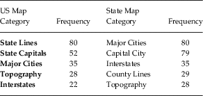
In the first phase of the research, 100 respondents filled in an empty map of the US and a state map of Georgia answering the following prompt: “Please look at the map below. Draw any information that you find important to make a map of Georgia (or USA). Moreover, label all of the information that you drew.” After the results were tabulated the top five most frequent categories were chosen for the second phase of the experiment. Table 1 below shows the frequency distribution among the top five categories.
Frequency distribution of the top five most important categories to be put on a basemap.

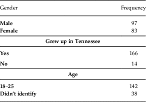
In the second phase of the research, a different group of respondents used five types of the US and the state of Tennessee maps created out of the five categories described above. Also, an empty map of the US and Tennessee were added (all basemaps in Appendix B). 180 respondents were asked to fill in maps with their perceptions. Each type of map was filled in by 30 respondents. Table 2 below shows the distribution of demographic information provided by the informants.
Distribution of demographic information about respondents.

As this distribution reveals, most of the informants were college age Tennesee natives, with an almost equal division between male and female.
The respondents’ paper maps were scanned, georeferenced, and digitized using a heads-up technique in ArcMap. The digitization process involved tracing polygons that covered the areas of perceptions marked by the respondents. Because each respondent defined an area, utilizing polygons, as opposed to polylines, was appropriate for this analysis. Each polygon was assigned with a text attribute from the text provided by the respondent on the map. Each respondent’s map was then saved as a unique feature class in a geodatabase. Additional attributes for classification were added and populated by analysis of the primary text string for each polygon.
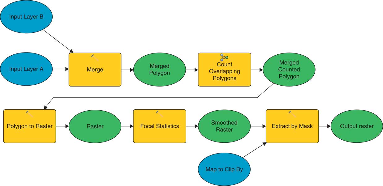
Respondent maps were processed for display by base map type, and for classification by use of an ArcGIS Model (See Figure 1). The model merges respondents’ maps, counts overlapping polygons and provides a smoothed raster output clipped at the extent of the map (Honeycutt, Reference Honeycutt2012). Raster smoothing was achieved by use of the Spatial Analyst plugin for ArcMap 10.3.1, using the tool focal statistics. Data smoothing is required for the analysis, and the process of spatial smoothing made interpretation of maps easier. By mapping the entire gradient (as opposed to creating an arbitrary threshold value), one can see the entirety of the data.
ArcGIS Model to merge multiple polygon vector feature classes into a single smoothed and clipped raster image.

Each continuous raster representing raw data containing all responses from a given basemap was converted to percentage agreement using the raster calculator. Each continuous percentage agreement raster was cast into an integer raster and the attribute table was exported to DBF file format and imported into Excel for analysis. The attribute table reflected the number of pixels of a given row value (percent agreement). The raw pixel data was converted to show the percent of the map each value covered.
Each map was graphed to provide a second means of visual assessment. Descriptive statistics including Features/n Z-Score, Kurtosis, and Skewness were calculated. A Pearson’s Correlation Matrix was performed to compare the similarities of each map.
3 RESULTS
3.1 National-level perceptions across all basemaps
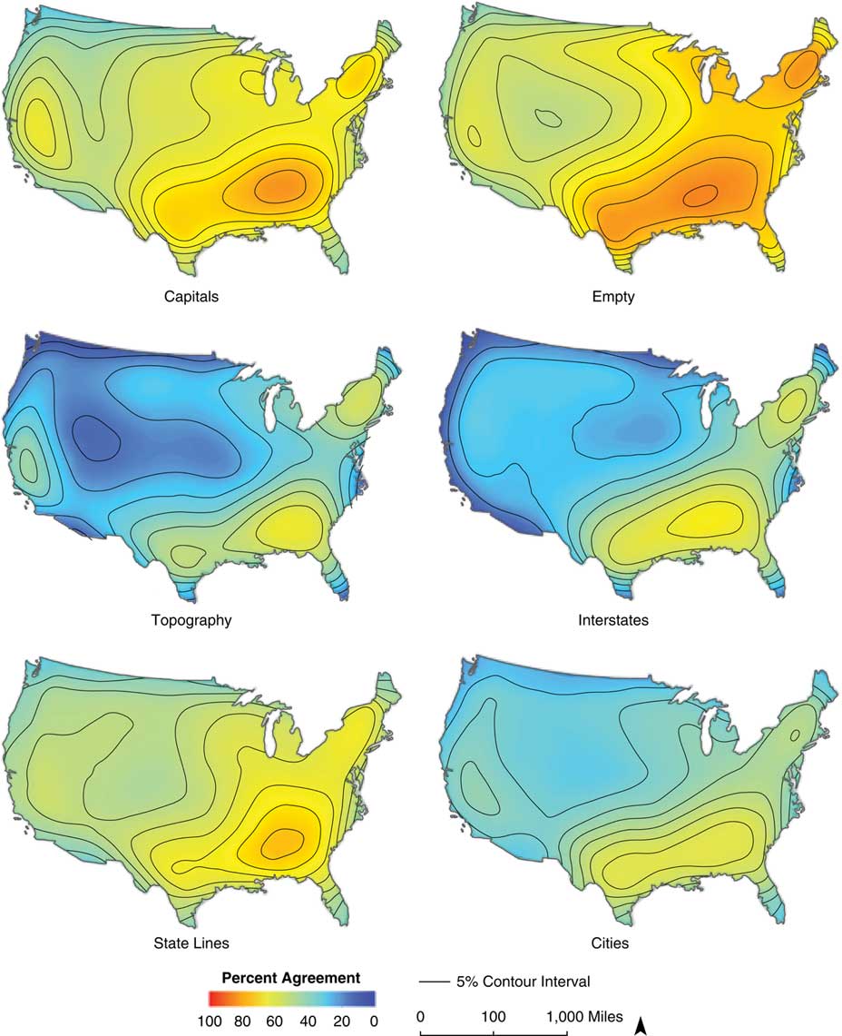
When all 180 national-level maps were collected and processed, each of the basemaps showed common patterns with the others, but also had unique features. None of the maps have areas that all the respondents indicated. Instead, the highest level of agreement ranges from 63% to 85% of the respondents agreeing on the areas presented in red on the maps below. This level of indication and its distribution indicates what many studies predict as variability in responses as well as production in the study of language (e.g., Kretzschmar, Reference Kretzschmar2009). We just don’t have the same ideas about the world around us, even on the large-scale cultural level, where commonly repeated patterns in education and popular culture reinforce cultural schemas. So, as we look at the results indicated below, we need to keep in mind that even for a pretty homogenous (in terms of demographic background) sample, we still have great variability that is reflected in the level and distribution of the perceptions. To illustrate the overall variability and low levels of agreement for even the most indicated areas, Figure 2 shows normalized levels of agreement for all six national basemaps. In this view, the red color indicates 100% agreement (which is not present on any map), and dark blue a 0% of agreement, which is present only on some maps and on small areas.
All national basemaps with normalized levels of agreement.

This normalized view across the basemaps shows us that the map that received the highest levels of agreement was the Empty basemap together with Capitals and State Lines. It also makes it visually clear that what we see most is the level of people not agreeing with each other more so than agreeing. However, to be able to talk about the patterns present in the results and where the respondents actually indicated their perceptual regions, the following GIS result basemaps will use the highest level of agreement to be indicated in red and the lowest level in dark blue. On the legend for each basemap we can see what those ends of the spectrum are.
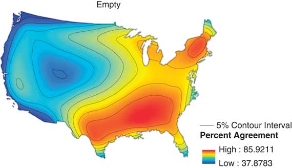
The Empty basemap (Figure 3), shows a large area of high-level agreement in the Southeast region of the US all the way to Texas, and another epicenter in New England.
National-level Empty basemap cumulative result map.

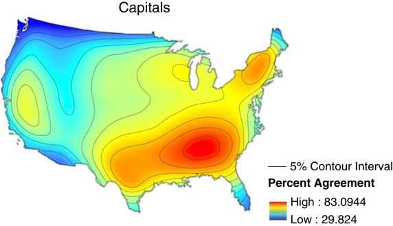
Contrary to Preston’s experiences, and confirming Lameli’s et al. (Reference Lameli, Purshke and Kehrein2008) findings, the respondents had no trouble filling in the Empty maps with their perceptions. According to Lameli et al. (Reference Lameli, Purshke and Kehrein2008), this basemap presented no bias, and yielded the most spontaneous results from the informants. I would add that what we see on the Empty basemap in the present research is lack of detail in the areas that are perceived as the most popular. The mid-to-high levels of agreement cover almost half of the country. So, it may be the case that without any anchoring information given on the basemap, respondents reach for the observational artifacts that are the most spontaneous, but may show the most variation in pinpointing them to a specific geographical location due to the lack of geographic markers. Moreover, we need to point out that the results on this basemap indicate that, despite the lack of information, informants are still able to put the Southerners in the South and Northeasterners in the Northeast. This must indicate that this basemap activates at least gross geographical and social concepts, and is a strong enough perception that, even without any markers on the map, appears commonly among the responses.
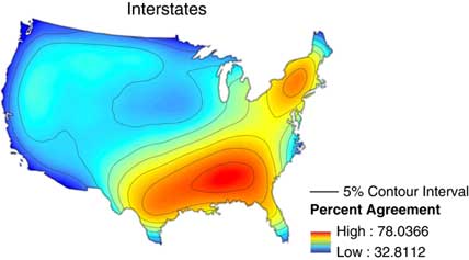
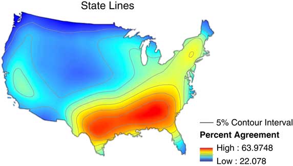
The Interstates (Figure 4) and State Lines (Figure 5) basemaps look very similar to each other, though they are both clearly different from the control basemaps.
National-level Interstates basemap cumulative results map.

National-level State Lines basemap cumulative result map.

In American PD, state lines on maps are almost considered a standard type of feature on basemaps, and, as shown in the first phase of this research, the most popular choice by informants in creating their “perfect” map. Although, as indicated earlier, even Preston (Reference Preston1989) concludes that those lines probably trigger stereotypes. Lameli at al. (Reference Lameli, Purshke and Kehrein2008) makes a stronger claim based on their findings, and point out that the state lines cause conceptual narrowing. In other words, the lines on the map activate the idea that a region encompassed in a state line has to have a specific perceived speech variety there, and the state lines correspond to the dialect boundaries. In that sense, we see the same process in the present research. Interstates and State Lines basemaps are maps with lines on them, and respondents use them. They not only typically trace those lines to indicate speech varieties, but also begin to indicate more detailed linguistic areas that otherwise might not have shown up.
The area that is almost identical between the Interstates and State Lines is the South. It stretches from the Southeast to cover Texas. As can be seen across all basemaps, the South is the most prevalent perceptual region, and although it may vary in its size between basemaps, the informants are sure that the South exists. The North can be seen on both basemaps, but the Interstates basemap provided a higher level of agreement in the area of New England. This might have been caused by a high congestion of interstates in that area used as delineations for perceptual regions. Those two basemaps seem to activate perceptions that are based on and connected to the premise that dialect boundaries do exist and the lines on the map correspond to them. This way, we see an example of Kretzschmar’s (Reference Kretzschmar2015: 150) claim that dialect areas are a product of our perceptions and not of the way we actually produce language; perceptual and production maps of dialect varieties do not correspond to each other. We can see this even if we just compare the first three basemaps, and acknowledge that each of them triggers different perceptions about language.
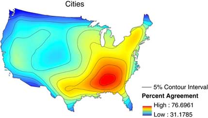
The Cities (Figure 6) and Capitals (Figure 7) basemaps provide us with another view of the collected perceptions. The Capitals basemap provides the state capital for each state, and the Cities basemap shows the 50 most populated cities in the US. Some of the towns show up on both maps.
National-level Cities basemap cumulative result map.

National-level Capitals basemap cumulative result map.

The results on those two basemaps look similar, although there are specific areas that differentiate them. Consistent with all other basemaps, the South is indicated on them, and a variety in the North. However, on the Capitals basemap we can also see an area on the West coast, while on the Cities basemap, we see a more restricted South, confined primarily to the Southeast part of the US, and not stretching westward to reach Texas.
According to Lameli et al. (Reference Lameli, Purshke and Kehrein2008), cities provide anchors or prototypes of regional languages and can also serve as language landscapes. This idea goes along with assertions provided by Kretzschmar (Reference Kretzschmar1996) that large cities, especially those on the East coast, provide cultural centers that radiate their influence outwards and, therefore, become a mental shortcut for a regional speech variety. We can see such an example on the Capitals basemap that displays a mid-level of agreement area on the West coast. Such recognition on the West coast appears only on one other basemap: Topography. Here, we follow Lameli et al. (Reference Lameli, Purshke and Kehrein2008) in positing that, since the cities are present on the map, they activate perceptions that otherwise would not be activated. In that way, they provide a different type of anchor for the regional varieties or language landscapes, with size as their differentiating characteristic.
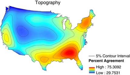
The last basemap presented in the present study was Topography (Figure 8). This basemap has general areas similar to all the others: The South, the North, and some indication on the West coast. However, the areas indicated seem to have sharper boundaries in comparison to the other maps.
National-level Topography basemap cumulative result map.

There are not that many areas in the mid-level of agreement as on the other maps. It may be explained by Lameli et al.’s (Reference Lameli, Purshke and Kehrein2008) observation that the topography only influences the responses when the perceived language areas and the topographical areas correspond. We can see on this map that what historically and culturally has been claimed about American English is reflected clearly on these maps. Respondents use the topographical information provided on the basemap; if it corresponds to the speech variety in mind, that information is used as an anchor. This map is different from all others in the type of markers provided on the basemap. It contains topographical information, so it is not like the Empty basemap. However, the information provided doesn’t have sharp boundaries such as the Interstate or State Lines basemaps, but the boundaries are more defined than points on the Cities or Capitals basemaps. That makes this map unique. Moreover, the Topography basemap results tend to most closely resemble the Empty map (except for the West coast speech area). Plotted responses look similar to those of the Empty basemap, but with more sharply defined areas, as if the respondents were more decided and sure where on the map to anchor their perceptions.
What we have seen in the results on all of the six different basemaps is that the respondents make different choices based on the information given on the basemap, but their choices, when aggregated, do resemble each other in the three most recognizable perceptual regions: the South, the Northeast, and West Coast. I believe that this contradiction can be explained by the ideas discussed in cultural geography (Zelinsky Reference Zelinsky1992, Gould and White Reference Gould and White1986) and echoed by Kretzschmar (Reference Kretzschmar2009): “At levels beyond the local, relative similarity of perceptions may arise from the lack of information that people have about other places, rather than from any actual shared perceptions. Thus an overall ‘average’ is likely to fail to capture actual similarities and differences in aggregated evidence of perceptions.” Therefore, what we see the informants do with the basemaps on the national level is to reach for the national-level cultural schemas associated with language varieties. Thus, we see the South, the Northeast, and West Coast as really the only three areas that receive high level of agreement. Those arise from shared cultural experiences, and not necessarily actual experience with speakers of those perceived varieties. However, we are still individual speakers. There is a great deal of variation in the way we construct those schemas, and so different basemaps “do” different things to our perceptions and activate various observational artifacts.
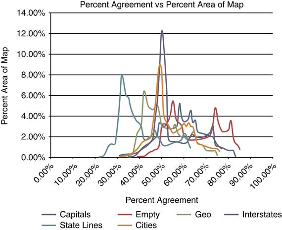
Moreover, statistical description of the data reinforces the patterns we have seen on the GIS maps. Figure 9 below shows the percentage agreement versus percent area of map for all six basemaps.
National-level map showing Percent Agreement vs Percent Area of Map.

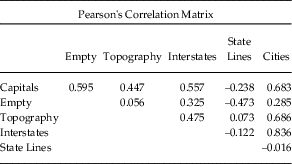
This figure shows on the x-axis the level of agreement that the respondents reached for all six types of basemaps. The y-axis indicates the amount of area covered by that level of agreement. So, the peaks show us where the bulk of agreement values appear on a map where the level of agreement is on the x-axis. For example, 8% of the State Lines map values show just over 30% agreement. What is important to point out is that the agreement that we are seeing in the chart is an agreement within the sample for each basemap. So, how well the respondents for each basemap agreed with each other, but only for each basemap, and not in comparison to others (the comparison is described below when we discuss Pearson’s Correlation Matrix). What Figure 9 shows us is that all of the maps together show a close to normal distribution shape, although the peak for Interstates is interesting, because it shows us a moderate level of agreement (about 50%) over the largest area (a little over 12% of the area of the map). The next closest peak is of the Cities basemap. Here we see a little below 50% level of agreement over an area covering about 9% of the basemap. This similarity between those two maps is confirmed when we look at the comparison of the basemap using Pearson’s Correlation Matrix. This matrix allows us to see how similar the basemaps are to each other. As the number approaches 1 the more similar basemaps are; the closer the number is to –1, the more dissimilar the basemaps are. Again, those similarities and differences are in regard to the internal consistency of the responses for each basemap, not necessarily indicating that the various maps have similar or different spatial distributions of the perceptions. Table 3 presents the correlation matrix for six basemaps on the national level.
Pearson’s Correlation Matrix for national-level basemaps.

What has been indicated in yellow is the greatest similarity between the State Lines basemap and the Cities basemap, a similarity in the highest peaks we have seen in Figure 9. What this indicates is that the respondents using those two basemaps showed the most consistency in indication of the perceptual areas, although they didn’t do it with a high level of agreement, instead with a moderate one (around 50%), and that makes those two basemap data sets most similar to each other, although not necessarily in the spatial distribution of the perceptions. On the other hand, the two chart areas in Figure 9 that are the most unlike each other are those for State Lines and Empty basemaps. Their peaks are very different with State Lines on the low level of agreement (right around 30%), and Empty basemap with peaks in 55%, 75%, and 82%, so moderate to high agreement. We can interpret this if we take into account a claim made earlier that the conceptually Empty basemap is very different from a State Lines basemap, because there are no features for the respondents to rely on within the Empty basemap, while the state lines provide convenient lines to use as boundaries while indicating perceptual areas.
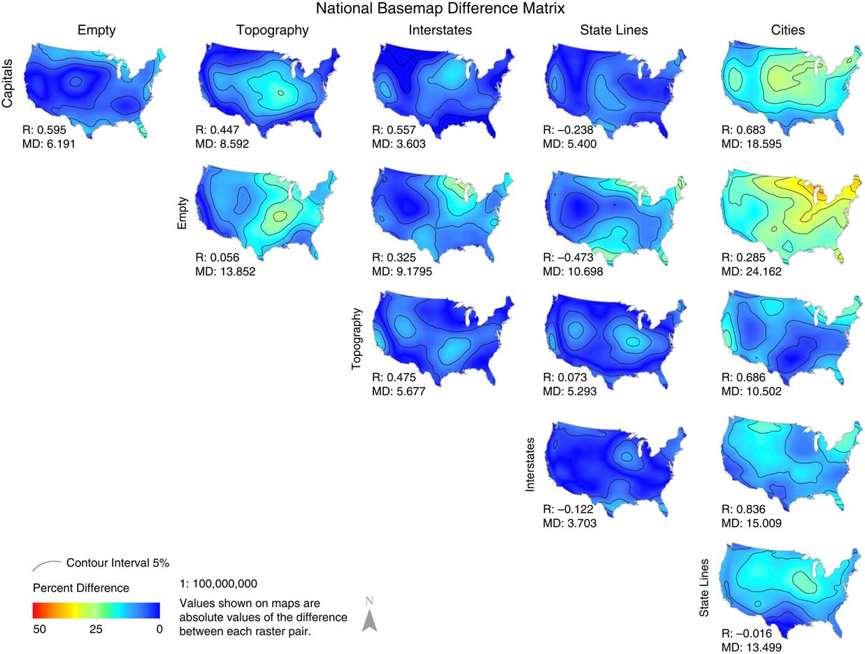
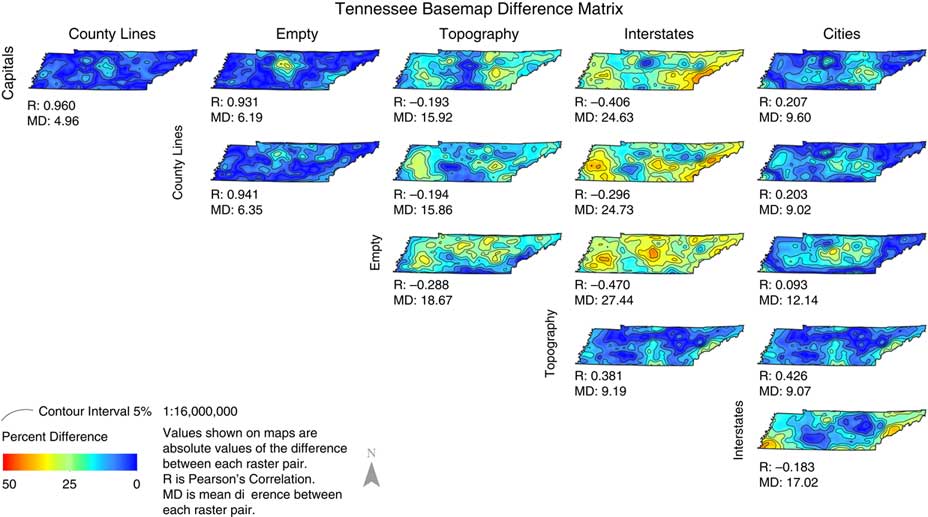
Since the statistical tests described above do not provide us with a visual representation of the spatial distribution of differences and similarities between the basemaps, we have created a difference matrix (in Figure 10) that displays the level of difference between basemaps in their spatial distribution.
National Basemap Difference Matrix.

In this matrix, we can compare the difference level between basemaps to see how various basemaps compared to each other in spatial distribution. Consistently with the observations in this whole section, we can see that on most maps the differences are not high, with a lot of the areas covered by the 0%–15% level of difference. This indicates as we have noticed before that the respondents reach for common cultural schemas in expressing their perceptions on the maps. Those culturally shared ideas seem to be consistent for this sample of the respondents. The one basemap that already has revealed its difference is the Cities basemap, and we see here as well that it is the most different from the Empty and Capitals basemaps. This visual representation allows us to see the higher level of consistency in the spatial distribution of the perceptual regions on the national level (the story is different for state-level basemaps, see section 5.2), which indicates that the respondents rely on culturally shared ideas and anchor them on the basemaps.
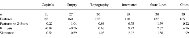
Lastly, to provide more descriptive statistical evidence, Table 4 shows results of more illuminating tests.
Statistical evidence for the national-level basemaps.

The first line (n) shows us how many maps were used for each of the basemaps (some of them are not 30, because some of the maps were empty). The second row (Features) shows the number of polygons indicated on each of the basemaps. We can see that those numbers are similar to each other between the basemaps; however, only row three (Feature/n) gives us a normalized comparison between the basemaps, in which the Empty basemap had more polygons than other basemaps, and State Lines basemap had fewer than any other. The next row provides us with yet another dimension connected to the peaks we saw for Cities and Interstates in Figure 9. In the kurtosis category that indicates how peaked the frequency is and that shows consistency between respondents in identifying the same regions, anything that receives a score larger than 3 is considered interesting. In the results we see that for Cities basemaps the number is 4.76, which makes it noticeable and higher than others, but it is the Interstate basemap that receives a score of 9.23 that makes this basemap very different than the others. For the Interstate basemap, the respondents not only agree with each other in the indication of the perceptual areas on a moderate level (indicated by the highest peak in Figure 9), but also the areas that they do indicate are the most alike out of all the basemaps. This may reinforce the idea indicated earlier that the interstates present on the basemaps are used to anchor the perceptual artifacts. The same, although with a smaller intensity, can be said about the Cities basemap. The last row deals with skewness of the data for each of the basemaps. The positive numbers indicate a low level of agreement within the basemaps overall true for all the basemaps, which shows that people just do not agree with each other about their perceptions, and the fact that even highest levels of agreement do not go over 85% on any basemap.
The descriptive statistics shown here allows a confirmation and complication of the visual representation of the spatial distribution of the perceptual areas. We have seen that there are patterns in the maps that make the features resembling lines different from others. We have seen a fuller vision of that in the Interstate basemap being an outlier from the other basemaps. At the same time, the Cities basemap came out as one that also seems to have its features influencing the respondents’ anchoring of their perceptual regions. We have seen in the spatial distribution on the Cities and Capitals basemaps that regions that otherwise don’t show up much on other maps do show up on those. However, it was in the descriptive statistic section that we have seen more of detailed portrayal of that for the Cities basemap. Now that the national-level maps have been described, it is time to see what patterns are present on the state level of Tennessee.
3.2 State-level perceptions across all basemaps.
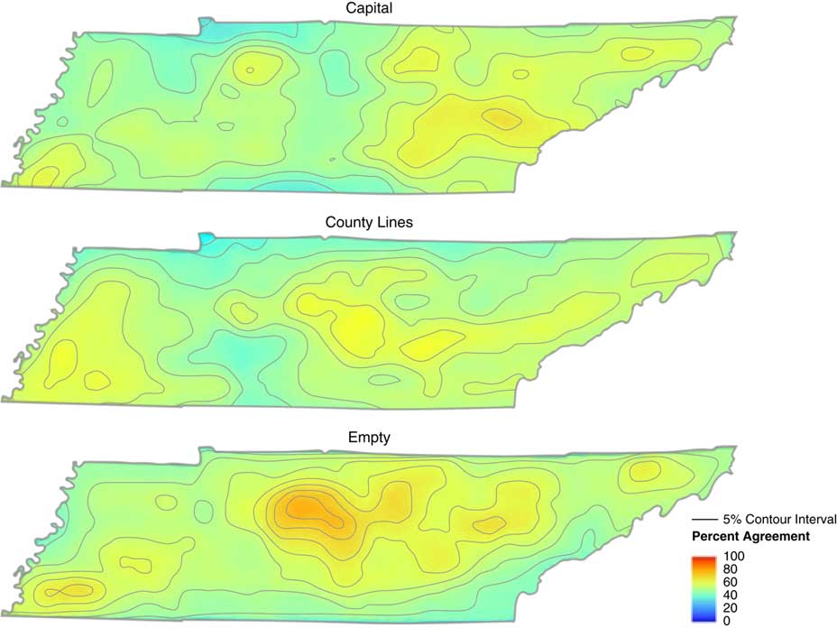
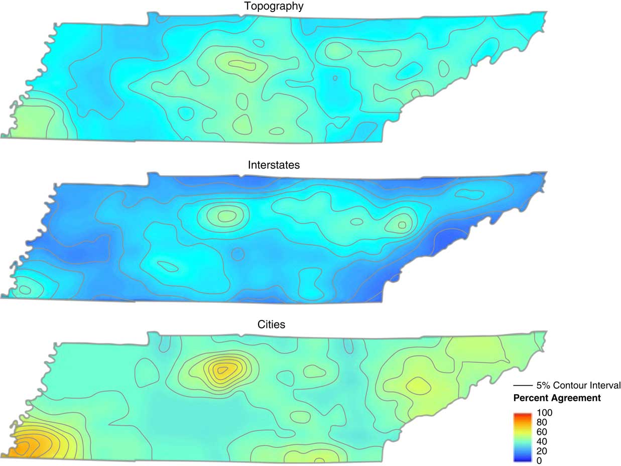
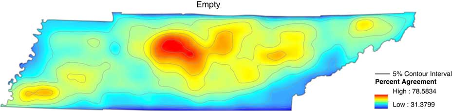
On the state basemaps of Tennessee, the situation is very different from the national results. For one, there are only a very few areas that appear on all basemaps with varying degrees of agreement. Those areas are located around Nashville and Memphis as Tennessee’s major urban areas. But even those are not that similar in the shape and level of agreement across all basemaps. Moreover, we see even a lower level of agreement on the most frequently indicated areas (in red on the maps). Here the range of the highest level of agreement oscillates between 47% to 81%. Again, such a wide range of the amount of agreement on the most popular areas shows us even greater level of variability in how the respondents see their own state. So, as we look through the various basemaps, we need to keep in mind that although all of them have agreed upon areas that the respondents see as the most prominent in their view, how many agreed on those will vary between basemaps. Yet again, to illustrate the low level of agreement present among the respondents, Figures 11 and 12 are presented below. The levels of agreement have been normalized across all basemaps, therefore red indicates 100% agreement (not present on any of the basemaps), and dark blue represents 0% of agreement (only present in small portions on the Interstate basemap).
Capital, County Lines, and Empty basemaps with normalized levels of agreement.

Topography, Interstates, and Cities basemaps with normalized levels of agreement.

As described above, the normalization across all basemaps does reveal that the levels of agreement are not that high. However, we also see, especially for maps in Figure 11, that there are large portions of the maps covered by similar levels of agreement. Again, just as we did for national-level basemaps, the following GIS result maps use the percent agreement but are normalized for each basemap. So, red indicates the highest level of agreement for that result map, and dark blue shows the lowest level of agreement. The actual levels are indicated in each legend. This allows us to see the regions that the respondents most frequently indicated on the maps, and we are able to talk about the emergent patterns.
The first result map shown is the Empty basemap (Figure 13). We can see a large area around Nashville and some pockets of higher level of agreement in middle and eastern Tennessee. The area around Memphis is small and doesn’t reach the highest level of agreement. This type of distribution may indicate that Nashville, as the state capital and cultural center of the state, receives the most recognition and even without it being marked on the basemap, it is prominent enough to appear on 80% of the maps.
State-level Empty basemap cumulative result map.

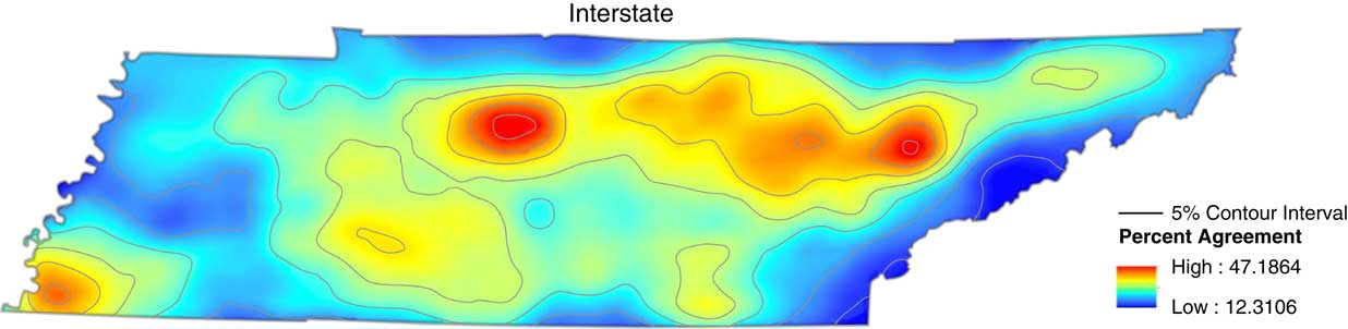
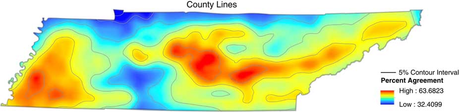
The distribution on the Interstate (Figure 14) and the County Lines basemaps (Figure 15) is not as similar on the state level as it was on the national level.
State-level Interstate basemap cumulative result map.

State-level County Lines basemap cumulative result map.

On the Interstate basemap we see some bias toward using I-40 (going east–west through the state) as a boundary, but the areas are in a form of pockets of high-level of agreement rather than larger areas where the highways are used as boundaries. This basemap is the first example of an occurring pattern of the respondents not using the markers on the maps to indicate their perceptions; in some cases, it was almost as if they were ignoring them on purpose.
The County Lines basemap again shows a high-level of agreement area in the middle Tennessee and partially in eastern Tennessee. This basemap has the largest area marked by the informants around Memphis although not on the highest level of agreement. Again, the county lines didn’t seem to be the features that swayed the respondents to specify their perceptions according to the lines on the basemap.
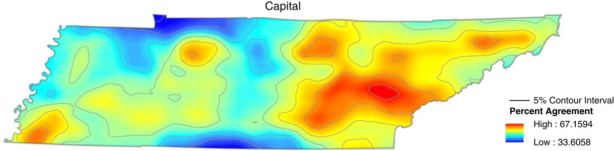
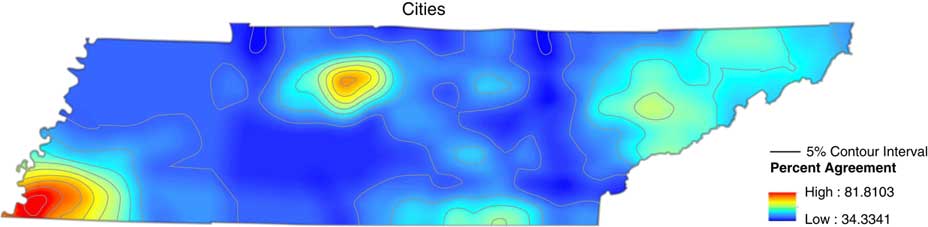
On the Capital (Figure 16) and Cities basemaps (Figure 17) the situation once again is very different from the national-level basemaps. The most surprising finding is that on the Capital basemap that only has Nashville marked on the map, the area around Nashville is the smallest and has received the lowest level of agreement among all basemaps.
State-level Capital basemap cumulative result map.

State-level Cities basemap cumulative result map.

The area that was most popular among the respondents was located in east Tennessee. In that sense, we can once again see that the details of the basemap didn’t seem to have any effect on the shape of the perceptions, and maybe even go as far as to say that the informants ignored the capital city marked on the basemap.
On the Cities basemap, which had the 50 most populated cities in Tennessee, we do not see much of an impact of that type of marker on the shape of the perceptions. On the national level we saw areas that didn’t get recognition elsewhere, but had cities marked to be used as perceptual anchors; however, here the only two high-level agreement areas are located around Nashville and Memphis with only a few pockets of mid-level agreement in east Tennessee. So, having 50 cities on the map didn’t really cause a lot of those cities to be the anchors of regional speech or create language landscapes like we saw on the national level.
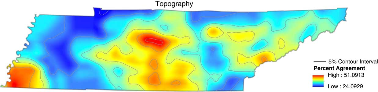
The last basemap, Topography (Figure 18), once again proved to have a different distribution of perceptual regions than all the other basemaps. The two hot spots were located around Nashville and Memphis, but we also have a type of corridor stretching from around Nashville south to the border with Georgia that didn’t exist on any other basemaps.Footnote 2
State-level Topography basemap cumulative result map.

The area that this mid- to high-level of agreement covers doesn’t actually have any specific markers on the basemap itself, which again allows us to speculate that the informants didn’t really use this map as a crutch to anchor their observational artifacts. Moreover, another surprising result that the Topography map shows is that the Appalachian Mountains that are marked and signed on the basemap only yielded a few small pockets of perceptual areas, although culturally the Appalachian region is commonly recognized as possessing a distinct speech.Footnote 3
As we have seen, state-level results point to a very different role that the basemap play in the way respondents use them to map their perceptions. On the national level, there were clear indications of what types of features on the basemaps sway the informants, and which ones are more neutral. However, on the state level there doesn’t seem to be any patterns beyond that the two biggest cities in Tennessee: Nashville and Memphis are somehow indicated on each type of map. Beyond that, the perceptual regions do not neatly overlap or fall into patterns. It is also hard to prove that the details provided on the basemaps are being used much at all by the informants. Just the opposite seems to be true: we see that Nashville receives the least recognition on the Capital basemap that has only Nashville marked on it. Having the 50 most populated cities in Tennessee marked on the map does almost nothing to create anchors for perceptions in places that otherwise wouldn’t have a chance to be indicated. We saw that having the Appalachian Mountains marked on the map didn’t trigger any major amount of perceptions to be anchored to that area, although culturally Appalachian is one of the commonly recognized speech varieties. And finally we saw that having lines on the maps in the form of interstates or county lines did little to push informants to use them as boundaries. This indicates that on a smaller scale where respondents have more experience (most of the respondents are native Tennesseans), the features provided on the basemap are not as important. They know what they know and whatever is on the map doesn’t have much influence on what they put on the map. Respondents do not have to rely on the high-level, national, shared cultural schemas. Instead, they can fully rely on their own, individual schemas that do not overlap as much with other speakers as they do on the national level.
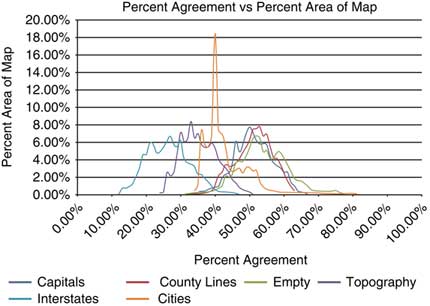
The variable relationship between the result maps is also seen in the distributions for all of the basemaps. Figure 19 shows the Percent Agreement versus Percent Area of Map.
State-level map showing Percent Agreement vs Percent Area of Map.

Just like we have seen in the distribution for the national-level basemaps (see Figure 9 above), we see mostly a normal distribution for all of the basemaps, except for the Cities basemap. The peak is even more dramatic than that of the Interstates on the national-level basemaps. Here we see that again we have a moderate level of agreement on the 40% level, but the area covered is a little over 18%. It is the biggest piece of a basemap covered by any level of agreement, showing a consistency not seen elsewhere. This distribution may be an indication that the Cities features do provide consistency not seen on other basemaps.
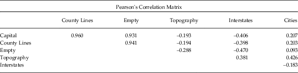
The differences between the basemaps (including the Cities map) are made clear when we look at the Pearson’s Correlation Matrix presented in Table 5 below.
Pearson’s Correlation matrix for state-level basemaps.

According to the results, the Empty basemap is similar in its consistency of responses to the Capital and County Lines basemaps, which can also be observed on the very closely distributed chart (Figure 19). This similarity does not necessarily translate into consistency in spatial distribution of perceptions. The three that are the most different from each other are Interstates, Capital, and Empty. Just as we have seen on the national-level basemaps, those most different from each other reside on opposite ends of the distribution. Therefore, the responses on the Interstate basemap only reach their peaks at about 30% level of agreement, while the other two hover over 50% level. The chart view provides us with ideas about the consistency in responses within those subsamples, but it doesn’t show us how much of an overlap there is in the spatial distribution of perceptual regions. However, Figure 20 shows the level of that difference.
Tennessee Basemap Difference Matrix.

Unlike the national-level matrix (Figure 10), here we see a lot of differences between the maps with only one comparison (County Lines and Capital) staying in the 0%–15% difference range. The rest of the pairings have regions that are in the 25% and above difference category. This matrix shows us in visual comparison what we have seen in the GIS maps above: the respondents do not agree on the same perceptual regions or use the features on the basemaps to guide them. The lack of pattern in the most indicated areas of individual maps is reinforced in the matrix view.
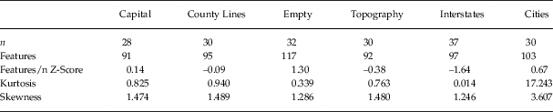
Lastly, Table 6 shows more statistical information to complete the view of the Tennessee basemaps. The categories of evidence are the same as we have seen on the national level (Table 4), but the distribution of the results has patterns of its own.
Statistical evidence for the state-level basemaps.

Interesting patterns can be seen in the Features category on the state level: the Empty basemap contained the most polygons and the Interstates basemap had the least. The next two rows show the most interesting results for the Cities basemap: in the Skewness category the basemap received low level of agreement, but as shown in the Kurtosis category, had the most consistently indicated areas. It may seem contradictory, but if we compare it to the results in Figure 19, we see that Cities has its peak at about 40% of agreement (so moderate level) at covering the most area (consistent with results of its Kurtosis category).
Although the Cities basemap once again comes out as an outlier that is different from others, the statistical evidence combined with the GIS maps show us that the state-level perceptions behave differently from the national-level. On more local maps, the respondents seem not to rely as much on the features of the basemaps. The visual representations as well as descriptive statistics allow us to provide a more complete image of the state-level perceptions and showcase that larger variability on the local level can be attributed to the more complex and complicated schemas that local respondents have about their immediate environment.
4 DISCUSSION
The research presented in this study shows that different basemaps yield different results, reinforcing the observation that what is on the basemap has an influence on what type of perceptions are triggered and put on the perceptual maps. This observation is concurrent with findings proposed by Lameli et al. (Reference Lameli, Purshke and Kehrein2008) that basemaps make a difference and that studies conducted using different basemaps are not yielding the same types of results. Lameli’s research only considered basemaps on the national level. This research contributes further considerations; the results demonstrate that on the state level the role of basemaps is very different. On the national level the basemaps features seem to be used as a guides to anchor respondents’ perceptions, while on the state level these details had less influence on perceptions.
On the national level, the most commonly distinguished areas were the South and the Northeast, and the location of those was predictable with relatively little variation in perceived shape and size. Let’s remember that 92% of the respondents were from Tennessee, so they have experienced the culture of the South; but, it is unknown how much they were exposed to experiences outside of the South. However, if we follow D’Andrade (Reference D’Andrade1995) and Kretzschmar (Reference Kretzschmar2009, Reference Kretzschmar2015) and consider the process of perception through the gestalt mechanism, the triggering of cultural schemas that become whole concepts, then we can see how the South or North can be created based on little or no information or experience. Since both speech and cultural regions are those that historically and socially have been most recognizable in the United States, it is no surprise that they are the most frequent perceptual regions indicated.
We see that the respondents don’t need to know much or anything at all about linguistic regions in the US to form an opinion about them and activate a schema that is ready to be used in the perceptual task. However, since they may have no experience with the dialect regions about which they have an opinion, they may not know where exactly to place details on the map. This is where the various basemap features come in handy. As observed on the Capitals and Cities basemap, markers on the basemaps are used as anchors for a variety that otherwise is not indicated. In other words, the cities indicated on these basemaps serve as guides to indicate a speech type on the West coast, which doesn’t appear on the other basemaps. Likewise, any types of lines, such as the state boundaries or interstates, served as delineating devices for the observational artifacts to be placed. This was true both in Lameli et al.’s (Reference Lameli, Purshke and Kehrein2008) results as well as in the current study. The descriptive statistics provide a confirmation of that pattern.
Moreover, what reinforces the strength of the Northeast/South division can be seen in the results of the Empty basemap. Here, no features are present to guide the location of the South and Northeast regions, but both once again appear as the most frequent areas. Such results can indicate that those concepts are so strong that even if no guide is offered by the basemap, they still have a presence. In that sense, they are also the easiest to “pull” and use when asked about linguistic and cultural perceptions. In other words, the cultural schemas associated with a long history of the Northeast/South division are the “low-hanging fruit” ready to be placed wherever the basemap features guide it to.
The results for the state basemaps demonstrate very different respondent behavior. Yes, each basemap yields various results as we have seen on the national level; however, unlike at the national level, there are no discernible patterns overlapping between basemaps. The only area that returns on all of the basemaps is situated around the two most populated cities in Tennessee: Nashville and Memphis. Other perceptual regions vary between basemaps, which was very easily observed in the difference matrix. This puzzling lack of pattern can be explained if we consider how those perceptions on the state level were possibly created. Once again, let’s remember that 92% of the respondents were from Tennessee and completed the maps at a university in Tennessee. Although it is possible that not all respondents spent their entire lives in the state, the demographic confirms they lived in Tennessee during their childhood and were at the time of the study attending college in Tennessee. Therefore, in comparison to their exposure to the language and culture in all of the United States, their experiences in Tennessee must be richer. They also will be more variable in the sense that each life will be experienced in an idiosyncratic way, because of the different communities to which the informants belong. If we take those conditions into account, we can see that while growing up, the schemas of their local speech, as well as speech in the state will have some overlap—this might be why Nashville and Memphis appear so commonly—but will also have so much variation. No two people experience the world, including language, in the same way. In addition, the richer their experiences and exposure to the speech varieties and people that use them are, the more nuanced and complex their schema will be. We can imagine that a person who lived their whole life in Tennessee and travelled around the state, talking to people in different locales, will have a more detailed and decisive idea about people’s speech in Tennessee. Moreover, if the same person has spent their life in Tennessee, no matter how much schooling or cultural education they may have, their ideas about speech varieties around the country without experiencing them firsthand will be more limited than their local knowledge. Therefore, we can see that the same person will fill in a national basemap and reach for the most common cultural schemas like the North/South division, but when asked about perceptions in their own state, their knowledge, ideas, perceptions, and therefore their schemas will be more complex and idiosyncratic.
This is not where the differences end. As much as on the national level we see a reliance on basemap features to guide placement of observational artifacts, on the state-level basemaps we do not see such reliance, rather there seems to be a sense a rebellion against or disregard of those features. We observed this specifically with the Capital basemap, where Nashville was the only indicated feature, the Nashville area received the least recognition out of all basemaps. On the Topography basemap, where the Appalachian region was indicated, we saw Appalachian speech receive little attention. On the Cities basemap no additional cities were recognized beyond the two largest metropolises. Such behavior reinforces the idea that the informants’ schemas about people and speech in Tennessee are strong and complex, and don’t need much “help” from the basemaps. The respondents know what they know and are decisive in how to use it regardless of the basemap features provided.
However, there must be geographically and culturally important features and markers that speakers associate with speech varieties in Tennessee. It seems though that those provided on the basemaps in this study didn’t seem as important to the respondents as the features on the national level. Anecdotally, it seems that the division in West, Middle, and East Tennessee is prominent in the communities in Middle Tennessee, so perhaps such a feature would serve as an anchor for the perceptions.
The results indicate that on the national level the effect of the features on basemap was a lot stronger. Therefore, when conducting surveys on the national level, the type of basemap will have a strong influence on the results; Lameli et al. (Reference Lameli, Purshke and Kehrein2008) and this study demonstrate how different basemaps guide respondents in different ways. An empty map appears to be a useful basemap to elicit the strongest and most spontaneous perceptions, while features resembling lines appear to invite conceptual narrowing. The indication of cities yielded mixed results, as it seems to anchor perceptions in a more specific geographical location, but on the state level, it does not seem to have much influence on the spatial distribution of the perceptions. We see that the higher the scale the map is in from the local experiences of respondents, the more influence the features on it will have on the shape and distribution of the perceptions. And although the basemaps used in Lameli et al. (Reference Lameli, Purshke and Kehrein2008) were not identical in features to those here, and didn’t have the same exact effect on the results, overall they both demonstrate influence. I believe that just like the language lives in culture, the features that are on basemaps have their cultural connections; therefore, to some extent we see American and German cultures reflected in the various basemaps.
In the end, the current study complicates the use of basemaps, and opens up a path for research on more levels of locality exploring the effects of different types of basemaps. For instance, do basemaps matter if our maps only show a region, city, or neighborhood? That type of question would be fascinating to test in presenting a fuller picture of the relation between basemap features and our perceptions.

APPENDIX B.
Basemaps used in the current research on the national and state level.