Introduction

The global hydrologic cycle is one of the major components of the climate system. In high latitudes there are interactions among precipitation, evaporation, river flow and sea ice. Reference Aagaard and CarmackAagaard and Carmack (1989) indicated that changes in fresh-water flow could alter the stability of the Arctic water column and thus affect ocean processes. A model study by Reference SemtnerSemtner (1984) found that potential modifications of river flow into the Arctic would not cause major changes in ocean temperature, salinity or sea ice. Reference Weatherly and WalshWeatherly and Walsh (1996) used an ocean-ice model and found that decreased river runoff into the Arctic Ocean affects sea ice more than increased runoff because the former changes vertical stability more effectively. They also suggest that the Semtner study may have underestimated the impact of changes in river flow because the ocean model underestimated the strength of the halocline.

In recent years, coupled atmosphere-ocean models have been developed to study the climate system. The spatial resolution of these models is large in comparison to the scales of many important processes, such as leads in ice packs and the hydrology of snowmelt runoff in mountainous regions. Both of these smaller-scale processes are important in the present study, the former because large high-latitude heat fluxes occur through leads, and the latter because it affects the timing and magnitude of fresh-water inputs to the ocean.

The purpose of this paper is to describe a new sea-ice ad-vection scheme and use it in a coupled atmosphere-ocean model to examine components of the hydrologic cycle in the Arctic Ocean. Of particular interest are the interactions among river flow, ocean salimity and sea ice. When climate models are used at dccadal-to-century time-scales, one assumes that the magnitude of any physical responses to changes within the coupled system will dominate any slow climate drift of the model. For example, am change in coastal salinity that occurs in response to anomalously high river flow should exceed any change that is associated with a long-term drift of the model’s mean salinity. This study is based on a 23 year simulation of the coupled atmosphere-ocean model in which flux adjustments such as those described in Reference Manabe, Stouffer, Spolman and BryanManabe and others (1991) are not used.

The Coupled Atmosphere-Ocean-Ice Model

The coupled atmosphere-ocean-ice model developed by Reference Russell, Miller and RindRussell and others (1995) is used in this study. The resolution is 4° latitude by 5° longitude. There are nine vertical layers in the atmosphere and 13 in the ocean. The atmospheric model’s source terms, such as radiation, surface interaction and condensation, are similar to those of Reference HansenHansen and others (1983). The atmospheric model includes the C-grid scheme of Reference Arakawa and LambArakawa and Lamb (1977) to solve the momentum equation, and Reference Russell and LernerRussell and Lerner’s (1981) linear upstream scheme to advect potential enthalpy and water vapor. The river-muling scheme of Reference Miller, Russell and CaliriMiller and others (1994) is used to move model-generated runoff within a gridbox downstream to the ocean.

The ocean model is described in Reference Russell, Miller and RindRussell and others (1995). It uses the linear upstream scheme of Reference Russell and LernerRussell and Leraer (1981) for the advection of heat and salt, solves the mass and momentum equations with a new C-grid scheme, and is initialized with temperature and salinity from Reference Levirus, Burgett and BoyerLevitus and others (1994). The model allows divergent mass flux, and has a free surface. Calculations based on the gradients of pressure, heat and salt are used to determine the flow of mass, potential enthalpy and salt through 12 straits that are too narrow to be resolved by the grid resolution. Fresb water is added directly to the ocean by precipitation or river flow.

There are two improvements to the Reference Russell, Miller and RindRussell and others (1995) model that are used in this paper. One is the inclusion of sea-ice advection, which is discussed in the next section. The second is the use of ocean-surface albedo based on Reference Briegleb and RamanathanBrie-gleb and Ramanathan (1982) which has been used in the United Kingdom Meteorological Office (UKMO) atmosphere-ocean model. In Reference Russell, Miller and RindRussell and others (1995), the global annual ocean and ocean-ice albedo, weighted by incident solar radiation, was 7.4%. The atmospheric component of the atmosphere ocean model, when integrated with climatological ocean temperatures and sea-ice concentrations, had a global annual net heat imbalance into the oceans and ocean ice of 7.4 W m⁻². When the larger UKMO ocean and ice albedo of 9.6% is used, the net heat imbalance into the oceans is reduced to 3.9 W m⁻², which helps to reduce the climate drift in the coupled model.

Sea-Ice Advection

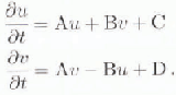
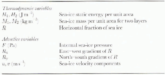
The new sca-ice advection scheme introduces five advective prognostic variables that are added to the five thermodynamic prognostic variables used in Reference Russell, Miller and RindRussell and others (1995) (see Table 1). The time rate-of-change of the sea-ice velocity components are given by

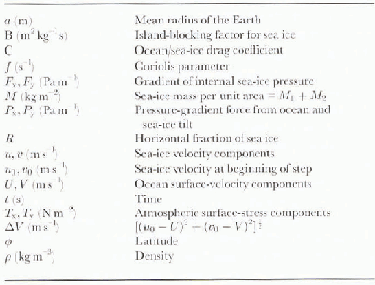
where the variables are defined in Table 2.

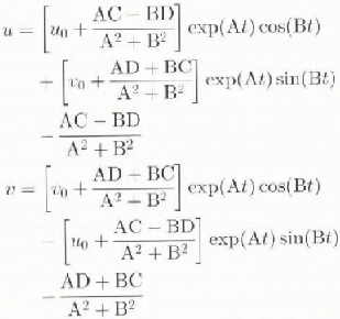
The equations for u and v are simultaneous linear differential equations:

They can be solved in closed form:

Table 1.

Prognostic variables for sea ice

Table 2.

Variables used by dynamical equations for sea ice

The sea-ice-velocity components are defined on the C-grid (i.e. they are defined perpendicular to the gridbox edges). This is ideal for sea-ice advection and for incorporating internal sea-ice pressures, but the Coriolis term is calculated less accurately. The pair of equations are solved twice, once for u using averaged values of v, and again for v using averaged values of u.

A modified linear upstream scheme (Reference Russell and LernerRussell and Lerner, 1981) is used to advect sea ice using the time-integrated velocities. The scheme produces smooth distributions of sea ice, yet is less diffusive than a standard upstream scheme.

The atmospheric-momentum stress for each component is assumed to be constant during an integration step of sea-ice velocity. The model’s minimum value of the sea-ice-ocean drag coefficient, “C” is 0.0012 for new ice. which is assumed to be 0.5 m thick. The coefficient is assumed to increase linearly with ice thickness, and is equal to 0.005 for 3 m thick ice (personal communication from D. Martinson, 1994). The time-integrated drag also accelerates the ocean below the ice. The island-blocking factor, “B”, is used to decelerate ice in regions where sub-gridscale-sized islands are present. The Coriolis and metric terms, for each horizontal velocity component, use a four-point average of the other horizontal velocity component. The components of the pressure-gradient force (P_x and P_y ) are caused by the ocean and sca-ice tilt and atmospheric pressure.

The calculation of internal sea-ice pressure F_x and F_y ) follows Reference Flato and HiblerFlato and Hibler (1992) with a few modifications. The prognostic internal sea-ice pressure is updated using an iteration scheme with at most 20 steps. In each step, the internal sca-ice pressure-gradient term is used in solving the two simultaneous linear equations for sea-ice velocity. The time integral of this sea-ice velocity estimates the sea-ice area crossing each gridbox edge. If the sea-ice area is convergent in a box, and the sea-ice pressure is below its maximum, then the ice-pressure increment is calculated so that the ice-area convergence would be zero were this increment the only change to the pressure field. If the sea-ire area is divergent in a box, and the sea-ice pressure is positive, then the ice-pressure increment is calculated so that the ice-arca divergence would be zero were this increment the only change to the sea-ice pressure field. The increments are applied to each gridbox before the next iteration.

The scheme used here causes sca-ice area convergence to approach zero, and applies all the pressure increments simultaneously at the end of an iteration. Gridbox order of calculations is unimportant. The largest increment for the 20th iteration in this implementation is usually less than 100 Pa. This scheme differs from that of Reference Flato and HiblerFlato and Hibler (1992) which causes sca-ice velocity convergence to approach zero, and applies the pressure increments as they are calculated for each gridbox. Their method converges more rapidly, but if convergence is not complete, then the order of calculations affects the results.

River Flow and Sea-Surface Salinity

The surface salinity of the Arctic Ocean is determined by water fluxes into the basin and mixing within the basin. The fresh-water budget of the Arctic Ocean depends on precipitation, evaporation, river flow, the advection of sea ice and interchange with other basins. Reference Miller and RussellMiller and Russell (1995) showed that the seasional variation of the model’s precipitation for the Arctic was similar to the observed precipitation of Reference Legates and WillmottLegates and Willmott (1990), with a maximum in the fall and a minimum in the spring. In this section we examine the potential effects of river flow on surface salinity.

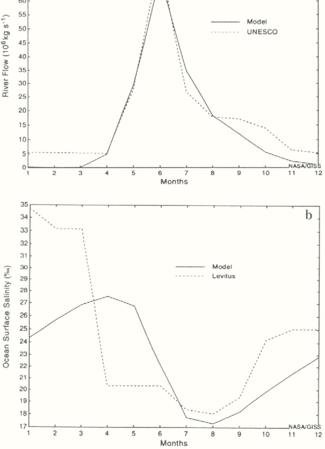
The ocean gridbox at the mouth of the Yenesei river is used to examine the local variation of sea-surface salinity at the mouth of a large river-system. This central Asian river is one of the largest rivers draining into the Arctic, and, as shown in Figure la, the model’s pronounced peak runoff from snowmelt in the spring is in good agreement with observations. Although Reference Mysak, Manak and MarsdenMysak and others (1990) found that Siberian rivers may not have the same impact on sea ice as the Mackenzic River in Canada, the Yenesei is examined here because the climate model represents its seasonal run-off significantly better than it does the Mackenzie’s.

Figure lb shows the model’s annual cycle of sea-surface salinity in the gridbox at the mouth of the Yenesei. Figure la and b shows that the model’s minimum salinity occurs during the two summer months following the maximum river flow in June. The decrease in salinity (10%₀) is consistent with what one should obtain by mixing the volume of fresh water into the top ocean layer, which is 12 m deep. Although the timing and magnitude of the model’s minimum salinity is the same as the observed, the model’s manimum salinity is the low, and occurs too late, compared to the observed winter-salinity maximum. It should be noted, however, that the Reference Levirus, Burgett and BoyerLevitus and others (1994) climatology for this location is based on sparse data during all seasons except summer.

Fig. 1.

Annual cycle of the models (a) river flow at the mouth of the Yenesei and (b) sea-surface salinity in the ocean gridbox at the mouth of The Yenesei, based on the last seven years of the model simulation. Also shown are the observed surface salinities based on Reference Levirus, Burgett and BoyerLevitus and others (1994) and the observed river flow based on Unesco (1985).

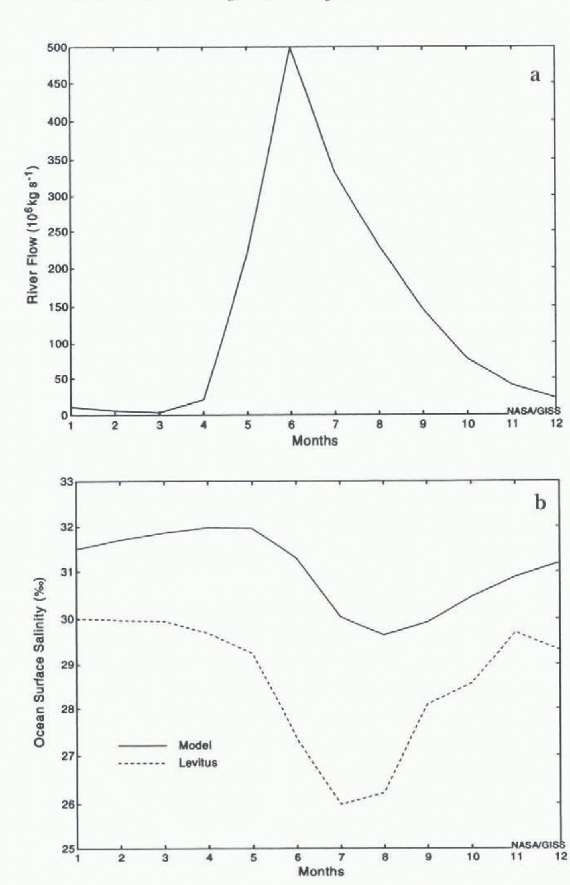
At the larger spatial scale. Figure 2a and b shows how the rurtoff into the Arctic Ocean, and the surface Salinity of the entire Arclic Ocean, vary through an annual cycle. The model docs attain its minimum salinity in the summer, consistent with the observed salinity variation, but the model’s salinity is too high and the annual range of salinity is about half the observed range of Reference Levirus, Burgett and BoyerLevitus and others (1994). Although further analysis is needed to determine win this occurs, it is probably due to excessive large-scale vertical mass fluxes at alternating gridboxes, or possibly due to excessive eonvective or diffusive vertical mixing.

Fig. 2.

Annual cycle of the model’s (a) river flow into the Arctic Ocean and (b) sea-surface salinity of the Aiclic Ocean based on the last seven years of the model simulation. Also shown are the observed surface salinities based on Reference Levirus, Burgett and BoyerLevitus and others (1994).

The inter-annual variability of river flow and salinity and their possible correlation is examined by calculating their seasonal anomalies. Figure 3a and b shows the model’s seasonal surface salinity anomaly at the mouth of the Yenesei and the entire Arctic Basin, respectively. Also shown is the seasonal river-flow anomaly. Locally, Figure 3a shows that the largest river-flow anomalies are followed by low salinity with approximately a 1–3 month delay. It is not clear that the same results hold for the entire basin. In fact, there is a downward trend in surlace salinity of the Arctic Ocean during this period.

Fig. 3.

Temporal variation of the anomalous seasonal surface salinity for (a) the gridbox at the mouth of the Yenesei and (b) the entire Arctic Ocean. Also shown is the seasonal rivei-flow anomaly, Based on the last seven years of the model simulation.

Sea Ice

The question examined in this section is whethcr sea ice and river flow are related. Figture 4a and b shows the seasonal cycle of sea-ice cover for the gridbox at the mouth of the Yenesei and for the entire Arctic Ocean, respectively. For the Yenesei, the model’s ice cover in the summer is too high, compared with the observed variation given by Reference Walsh and JohnsonWalsh and Johnson (1979). When the previous eight years of the model simulation were examined, the ice cover in the summer decreased to the same as the observed. Further analysis is needed to understand why the model’s summer iee cover in this gridbox has increased so much from the previous period. For the Arclic Ocean, the model and observed minima of ice cover occur in September. However, the model has too much ice in the summer.

Fig. 4.

Annual cycle of the model’s fractional ocean ice cover for (a) the Yenesei and (b) the entire Arctic Ocean based on the last seven years of the simulation. Also shown is the observed ice cover based on Reference Walsh and JohnsonWalsh and Johnson (1979).

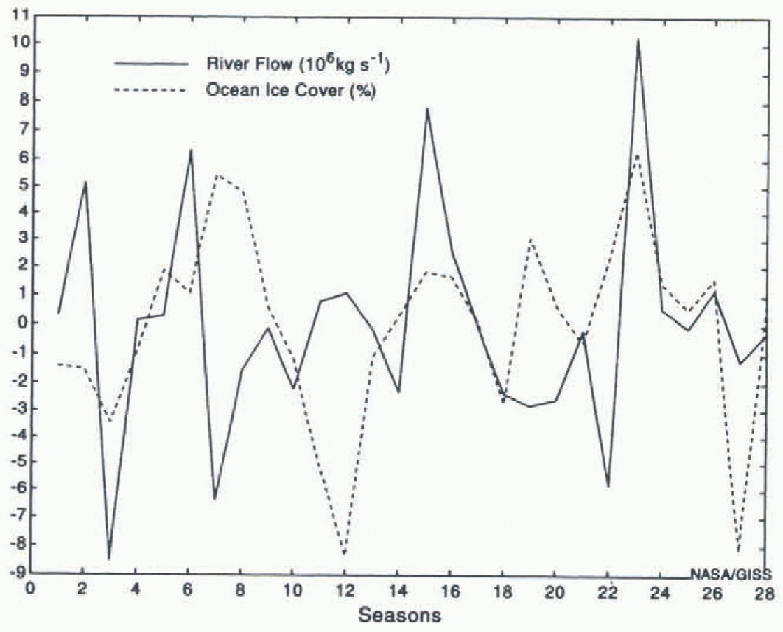
Figure 5 shows the seasonal anomalous river flow and sea-ice cover for the ocean gridbox at the mouth of the Yenesei. One might expect that years with anomalously high summer river flow would decrease the salinity sufficiently to allow water to freeze more easily the following fall, and thus be correlated with higher sea-ice cover in subsequent seasons. However, the figure shows that the sea-ice cover at the mouth of the Yenesei is not highly correlated with river flow. A similar result holds at the larger scale of the entire Arciic Basin. The additional effects of temperature must also be considered when examining sea-ice cover.

Fig. 5.

Temporal variation of the anomalous seasonal ice cover and seasonal river flow for the gridbox at the mouth of the Yenesei during the last seven years of the simulation.

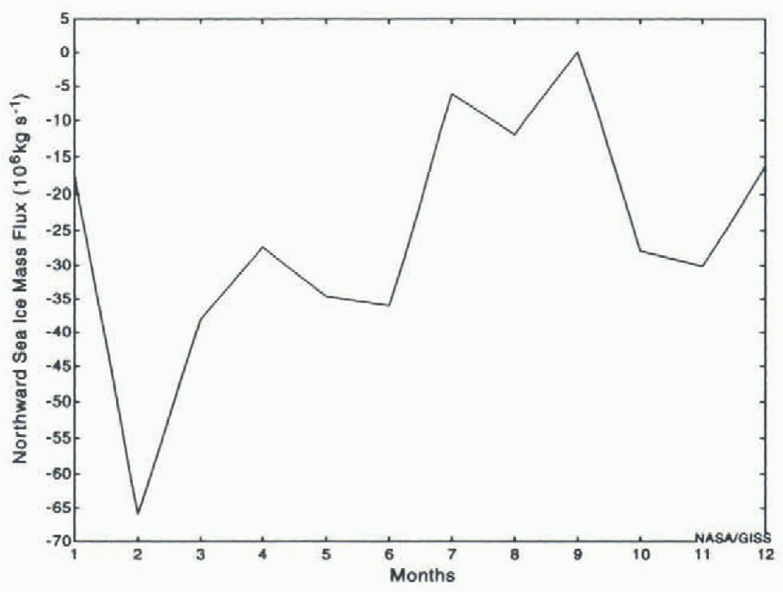
In addition to temperature and salinity, ice cover in a particular gridbox depends on whether ice is advected into or out of it. In fact, one mechanism for the removal of fresh water from the Arctic- Basin is by the advection of sea ice through Fram Strait. Figure 6 shows the model’s annual cycle ofice flow through Fram Strait. The seasonal cycle shows that the model’s maximum southward transport occurs in the late winter and early spring. However, the model’s mean annual southward transport is less than half of the 2790 km³ found by Reference Aagaard and CarmackAagaard and Carmack (1989).

Fig. 6.

Annual cycle of tha model’s northward flow of sea ice through Fram Strait. Based on the last seven years of the simulation.

The anomalous river flow into the Arctic was also examined to determine whether years of high runoff into the Arctic were followed by anomalous flow through Fram Strait. Reference Mysak, Manak and MarsdenMysak and others (1990) hypothesized that the “great salinity” anomaly might be related to high river fIlow into the Arctic, particularly from the Mackenzie River. Since no such correlation was found at the mouth of the Yenesei, it is not surprising that no such correlation has been found for the entire Arctic Basin. The relatively short time period examined here, and model deficiencies, however, could account for this finding. A longer simulation, with finer horizontal grid resolution, improved vertical-mixing processes, improved river flow and reduced climate drift should be examined.

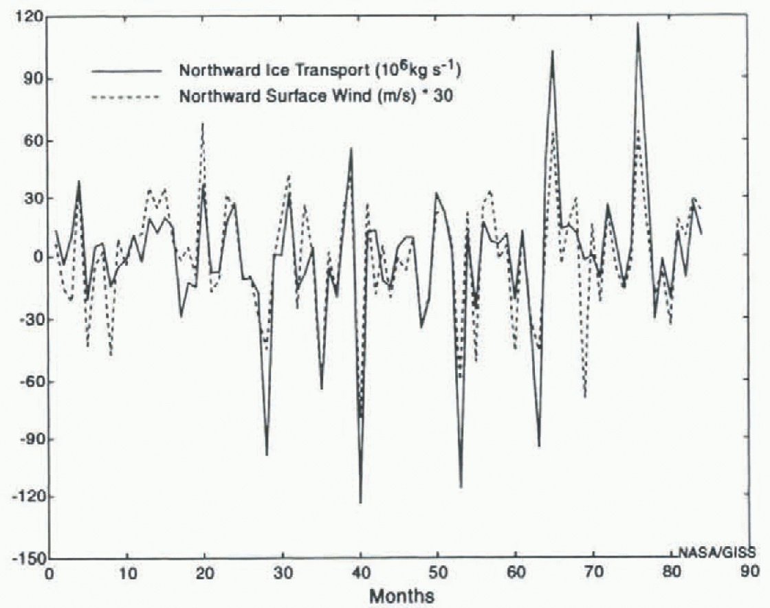
If the anomalous ice advection is not correlated with fresh-water inflow to the Arctic Basin, are there other physical variables with which it might be correlated? Figure 7 shows that the anomalous monthly sea-ice flow through Fram Strait is highly correlated with the anomalous meridional wind speed at the latitude of Fram Strait. The correlation coefficient is 0.81. When the wind is anomalously strong and southward (northward), the ice flow is anomalously high and southward (northward).

Fig. 7.

Anomalous flow of sea ice northward through Fram Strait for each month of the model simulation. Also shown is the model’s anomalous northward and wind speed.

Discussion

A model simulation with a global coupled atmosphere-ocean model and realistic river flow has been used to examine the effect of river flow on salinity and sea ice in the Arctic Ocean. The coupled model includes a new sea-ice advection model discussed in a previous section. Although the coupled model and the river flow do not represent the present climate system perfectly, there are a number of results that can be useful for further model development, and for examining potential physical processes in high latitudes.

Locally, the model shows that river flow does affect salinity at the mouths of large rivers. For the river Yenesei, the high summer runoff lowers the surface salinity at the mouth, consistent with observations. When the river flow is significantly higher (lower) than normal, anomalously low (high) salinity occurs in the adjacent coastal area. However, other physical processes, such as ocean or ice transport, also affect the surface salinity.

The model’s corresponding relationships between high runoff and increased ice cover are less clear. Reference Mysak, Manak and MarsdenMysak and others (1990) found that increased river flow from the Mackenzie River is positively correlated with sea-ice extern in the Beaufort Sea. The results of the presenl study are more supportive of the results of Reference WeatherlyWeatherly (1994) and Reference Weatherly and WalshWeatherly and Walsh (1996): an ocean-ice model showed that increased river runoff did not have a significant effect on sea-ice thick-ness, primarily because the runoff acted to strengthen an already strong halocline in most regions. They did find a greater impact on sea-ice thickness when river flow was reduced. Of course, ice formation also depends on temperature, which has not been examined here.

The sea-ice advection model developed for this study was also used to examine anomalous ice flow through Fram Strait into the Greenland-Iceland-Norwegian (GIN) Sea. The “great salinity” anomaly is an example of a high-latitude phenomenon that has been suggested depends on anomalies in the Arctic water budget (Reference Dickson, Meincke, Malmberg and LeeDickson and others 1988; Mvsak and Power, 1992). The model’s anomalous fresh-water inflow to the Arctic was not definitively correlated with sea-ice flow into the GIN Sea. The sea-ice flow through Fram Strait was highly correlated with the local meridional wind stress. This is consistent with the results of Reference Walsh and ChapmanWalsh and Chapman (1990), who calculated an atmospheric-pressure index between southern Greenland and the Arctic Asian coast, and found that its maximum value, which occurred in the 1960s, was consistent with enhanced wind forcing of older ice from the Arctic through Fram Strait. It is also consistent with the results of the model study of Reference HäkkinenHäkkinen (1993), who found that large ice exports from the Arctic were related to an anomalously strong low-pressure region in the Iceland Sea region. Addilional study is needed to determine whether years of high southward ice flow are associated with lower surface salinity in the GIN Sea. This is somewhat difficult to do with this model simulation, because the ice flow through Fram Strait is so low.

The results here are based on a coupled model that incorporates many different components of the hydrologic cycle to examine their interactions at high latitudes. Additional model improvements and longer simulations are needed to examine some of these results further and, in particular, to study interdecadal variability.