



Introduction
Asymmetric feeding current and non-uniform inter-element spacing allow for the creation of systems with higher degrees of freedom studying array pattern strategies – that is, lowering sidelobe level (SLL) while keeping beam width – has become more critical due to the increasing pollution of the electromagnetic environment. Concentric circular antenna arrays (CCAAs) have dramatically impacted communication via wireless networks, which may produce directed radiation patterns with a low loss yet significant gain, and in [Reference Balanis1, Reference Elliot2], the authors explained the geometrical configuration of an antenna array. The array’s circular shape guarantees even power distribution in every direction, making it perfect for omnidirectional coverage applications like wireless networks, satellite communication, and radar detectors to reduce performance loss in the signal-to-noise ratio due to undesired interference. While uniformly stimulated, evenly spaced antenna arrays often have high SLL, they also have good directivity. The Dragonfly algorithm in [Reference Babayigit3] optimizes the arrays’ components’ excitation amplitude and inter-element separation to lower the SLL.
Recently, a great deal of research has been done on CAAs to enhance their performance concerning radiation patterns, beam shaping, polarization diversity, and bandwidth for various antenna arrays and multiband CCAAs introduced in [Reference Elsanousi, Abbas, Hirtenfelder, AbdAlhameed, Yang, Le and Nguyen4]. It is necessary to build antennas with highly directional qualities to meet the need for communication over long distances in various scenarios. Radiating components are combined electrically and geometrically to form an antenna array. The Jaya algorithm is used in [Reference Thadikamalla and Rao5] to mitigate the SSL, and the addition of the vertically emitted fields from each component results in the overall field of the antenna array. Every element is arranged in a circular array around the circle’s edge. In [Reference Babayigit and Abubaker6], compared to other array forms, circular arrays have become more and more popular lately since they provide 360-degree azimuth coverage and can perform scans in all directions without appreciably altering the beam pattern. Furthermore, circular arrays are less prone to mutual coupling than linear and rectangular arrays since they do not have edge components and mutation hill climber cleared in [Reference Chinnasamy, Ramachandran, Amudha and Ramu7] and wide-angle scanning of CCAA expressed in [Reference Junqing, Xia and Zhu8, Reference Durmus and Kurban9].
This approach presents an effective technique to enhance the far-field radiation pattern of CCAAs by employing two stochastic optimization methods: the Social Spider Algorithm and a modified version, the Modified Social Spider Algorithm [Reference Wang, Chen, Qu, Lou and Luo10]. The Political Optimizer, a new socio-inspired meta-heuristic technique, is applied to enhance the far-field radiation properties of CCAAs. This approach aims to improve the key aspects of wireless communication for smart grids and the Internet of Things by minimizing the SLL, a crucial factor in the antenna’s radiation pattern time modulated and vertex radar introduced in [Reference Yesilyurt, Arican and Aksoy11, Reference Yang, Shi, Guo, Wang, Liu and Cheng12].
This article’s primary objective is to maintain low SLL. These two fundamental CAA design requirements are met by choosing the ideal current amplitude excitation and inter-element spacing and keeping a zero-phase difference between elements. In a study [Reference Das, Mandal and Kar13], for a compact circular antenna array design, a random optimization methodology known as krill herd optimization is used to synthesize an ideal far-field radiation pattern utilizing the time modulation method. The difficulties and potential paths for concentric ring array research are also covered in this work. Pareto multi-objective genetic method introduced in [Reference Devisasikala and Thiripurasundari14] and OAM antenna design and large antenna designs presented in [Reference Jie, Fan, Lu, Hu, Xie and Huang15, Reference Peng and Wang16], as well as Novel Particle Swarm Optimization (NPSO) and Particle Swarm Optimization (PSO) introduced in [Reference Thadikamalla Nageswar and Rao17, Reference Kazanskii, Vasquez-Peralvo and Chatzinotas18], employing a hybrid optimization approach to increase directivity and decrease SLL in [Reference Mittal, Sharma, Thangarasu, Sarat, Hourani and Salgotra19]. Non-uniform CCA using IPSO and MABC algorithm to minimize the SLL introduced in [Reference Zanganeh and Oskouei20, Reference Sun, Sun and Lei21] and Whale Optimization Algorithm (WOA) in [Reference Kundu, Bera and Pathak22]. This proposal utilizes the PSO, NPPSO, Jaya, and Craziness-based Particle Swarm Optimization (CRPSO) methodologies to modify the radiation pattern of both the SLL and first null beam width (FNBW) by adjusting the antenna elements’ input current values and inter-element separations. The objective is to achieve a maximum decrease in these parameters. When applied to a broad spectrum of applications, the CRPSO approach is highly effective in addressing directivity, effective aperture, and beam area issues. The remaining sections of this paper are organized as follows: The mathematical formulation of the CCAA provision provides a precise mathematical representation of the CCAA. The formulation of the fitness function section gives a concise overview of how the fitness function is formulated. The applied optimization techniques section discusses the optimization approach used for CCAA design. The numerical analysis and simulation results section explains the numerical analysis and simulation findings. Finally, the paper concludes with a summary of key insights.
Mathematical descriptions of non-uniform CCAA
In general the far-field pattern of an N-element array of isotropic elements can be described broadly as
 \begin{equation}
AF(\theta ,\phi ) = \sum\limits_{n = 1}^N {I_n e^{j(\alpha _n + kR_n {\rm{a}}_{\rm{r}} )} }
\end{equation}
 $I_n$ is the excitation amplitude coefficient of the
 $n^{th}$ element,
 $k$ is the wave number,
 $\alpha _n$ is the relative phase of the
 $n^{th}$ element,
 $R _n$ is the position of the element or vector of the
 $n^{th}$ element, and the unit vector is denoted as
 $a _r$. Figure 1 depicts the general array design of CCAA with
 $M$ concentric rings lying in the
 $x$–
 $y$ plane. In Figure 1,
 $r _m$ is the ring radius of the
 $m^{th}$ ring
 $(m=1,2,3...M)$ and the corresponding element in the respective ring is
 $N _m$ [Reference Kundu, Bera and Pathak22, Reference Li, Sun, Wang, Zheng, Chen, Liang and Liu23]. Far-field radiation pattern of non-uniform CCAA is given by:
 \begin{equation}
AF(\theta ,\phi ) = \sum\limits_{m = 1}^M {\sum\limits_{n = 1}^{N_m } {I_{mn} } } e^{j(kr_m {\sin} (\theta )\cos (\phi - \phi _{mn} ) + \alpha _{mn} )}
\end{equation}
Geometrical representation of non-uniform CCAA.

 $I_{mn}$ is the excitation amplitude coefficient of the
 $n^{th}$ element in the
 $m^{th}$ ring.
 \begin{equation}
I_{mn} = \left\{{_{0}^1 } \right.{}_{OFF}^{ON}
\end{equation}
Where  $k$ is the wave number
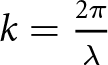 $k = {{2\pi } \over{{\lambda}} }$,
 ${\lambda}$ directs the wavelength,
 $\theta$ is the incident angle of the wave,
 $\phi $ is the azimuthal angle of the wave,
 $\phi _{mn}$ is the angular beam spot of the
 $n^{th}$ element in the
 $m^{th}$ ring, and
 $\alpha _{_{mn} }$ is the excitation phase of the
 $n^{th}$ element in the
 $m^{th}$ ring.
 \begin{equation}
\phi _{mn} = {{2\pi (n - 1)} \over {N_m }}
\end{equation}
 \begin{equation}
\alpha _{_{mn} } = - kr_m {\sin} (\theta _0 )\cos (\phi _0 - \phi _{mn} )
\end{equation}
 $\theta _0$ is the angle of the main peak of the radiation pattern
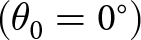 $(\theta _0 = 0^ \circ )$,
 $\theta$ varies from
 $
- 90^{\circ}$ to
 $90^{\circ}$ with maximum radiation at angle
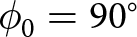 $\phi _0 = 90^{\circ}$. The normalized power pattern of the CCAA is given by
 \begin{equation}
P_{normalized} (\theta ,\phi ) = 20\log \left[ {{{\left| {AF(\theta ,\phi )} \right|} \over {\left| {AF(\theta ,\phi )} \right|_{\max } }}} \right]
\end{equation}
The directivity 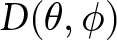 $D(\theta ,\phi )$ of the CCAA is expressed as
 \begin{equation}
D(\theta ,\phi ) = {{P_{normalized} (\theta ,\phi )} \over {{1 \over 4}\int\limits_{0}^{2\pi } {\int\limits_{0}^{\pi} {P_{normalized} (\theta ,\phi ){\sin} (\theta )d\theta d\phi } } }}
\end{equation}
In (7)  $P_{normalized} (\theta ,\phi )$ indicates the power radiated in the particular direction
 $(\theta ,\phi )$.
 ${1 \over 4}\int\limits_{0}^{2\pi } {\int\limits_{0}^{\pi} {P_{normalized} (\theta ,\phi ){\sin} (\theta )d\theta d\phi}}$: In order to provide dimensionless directivity that is based on the isotropic radiation, the pattern is normalized. The effective aperture
 $(A_{eff} )$ is expressed as the following equation [Reference Bera, Kundu and Pathak24]:
 \begin{equation}
A_{eff} = {{D(\theta ,\phi ) \times {{\lambda}}^2 } \over {4\pi }}
\end{equation}
Where 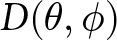 $D(\theta ,\phi )$ is the directivity of the antenna,
 $(A_{eff} )$ is the effective aperture (in square meters), and
 ${\lambda} $ is the wavelength of the incoming signal or wave (meters). The beam area
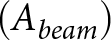 $(A_{beam})$ in steradians is given by
 \begin{equation}
A_{beam} = {{4\pi } \over {D(\theta ,\phi )}}
\end{equation}
Where 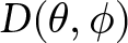 $D(\theta ,\phi )$ is the directivity of the antenna and
 $4\pi $ is the surface area of a unit sphere (radius = 1), which corresponds to the total solid angle surrounding a point.
The formula for determining a metric,  $FF$, is represented by Equation (10). It seems to be a combination of several weighted components and discrepancies between computed and reference values. The formula for determining a metric, fitness function (
 $FF$) [Reference Kumar, Ram, Mandal and Kar25], is represented by the following equation:
 \begin{equation}\begin{aligned}
FF = & \, W_1 \frac{|AF(\theta_{msl1},I_{mn}) + AF(\theta_{msl2},I_{mn})|}{|AF(\theta_0,I_{mn})|} \\
& + W_2 |FNBW^{Computed} - FNBW^{(I_{mn}=1)}| + \frac{1}{DIR} \\
& + W_3 (C_{01} - C_{R1}) + W_4 (C_{02} - C_{R2}) + W_5 (C_{03} - C_{R3})
\end{aligned}
\end{equation}
Where: In Equation (10) 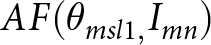 $AF(\theta _{msl1,} I_{mn} )$ specifically calculates the value of the array factor (AF) at the angle of the first maximum SLL, for a given set of excitation amplitude
 $I_{mn}$.
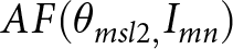 $AF(\theta _{msl2,} I_{mn} )$ specifically calculates the value of the AF at the angle of the second maximum SLL, for a given set of excitation amplitude
 $I_{mn}$.
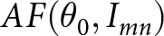 $AF(\theta _0 ,I_{mn} )$ represents the AF evaluated at the angle of the main beam, for a given set of element excitation amplitude
 $I_{mn}$ and
 $W_1$ is weight factor that is
 $W_1 = 0.096$. The SLL, a crucial performance indicator for antenna arrays, is measured using this term.
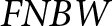
 $FNBW^{Computed}$ is the computed or calculated value of
 $FNBW$.
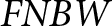
 $FNBW^{(I_{mn} = 1)}$ is the reference value of
 $FNBW$ when
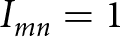 $I_{mn} = 1$, the absolute difference between these two values is taken, indicating how far the computed value deviates from the reference.
 $W_2 $: Weighting factor that is
 $W_2 = 0.044$ scales this difference to control its influence on
 $FF$ and
 $DIR$ is directivity. The third weight factor, which is chosen as
 $W_3 = 0.055$,
 $C_{01}$ is the computed circumference, and
 $C_{R1}$ is the required circumference.
 $W_4$ is the weight factor four, taken
 $W_4 = 0.059$,
 $C_{02}$ is the calculated circumference, and
 $C_{R2}$ is the required circumference.
 $W_5$ is weight factor five and it taken
 $W_5 = 0.089$,
 $C_{03}$ is computed circumference, and
 $C_{R3} $ is required circumference.
Employed optimization techniques: CRPSO algorithm
Because of improvements made to the traditional PSO, which have strengthened its ability to search globally, a modified version called CRPSO has been created. The velocity, in this case, may be shown as follows [Reference Kumar, Ram, Mandal and Kar25, Reference Thadikamalla and Amara26]:
 \begin{equation}
\begin{aligned}
V_i^{(k + 1)} &= r_2 \times sign(r_3 ) \times V_i^{(k)} \\
&\quad + C_{11} \times r_1 \times (1 - r_2 ) \times \{pbest_i^k - S_i^k \} \\
&\quad + C_{22} \times (1 - r_1 ) \times (1 - r_2 ) \times \{gbest^k - S_i^k \}
\end{aligned}
\end{equation}
The arbitrary parameters  $r_1$,
 $r_2$, and
 $r_3$ are randomly picked from the interval [0, 1], and the function
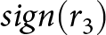 $
sign(r_3 )$ is defined as follows:
 \begin{equation}
\text{sign}(r_3) =
\begin{cases}
1, & r_3 \gt 0.05 \\
-1, & r_3 \leq 0.05
\end{cases}
\end{equation}
Notably, the two random parameters in (11),  $r_1$ and
 $r_2$, are independent. Personal and social experiences are highly dependent upon when both parameters are large, which frequently pushes the particle beyond the local optimum. In contrast, these experiences are underused when both parameters are tiny, which slows down the technique’s rate of convergence. To solve this problem,
 $r_1$, a single random number, is chosen instead of independent
 $r_1$ and
 $r_2$. This selection guarantees that
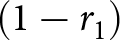 $(1 - r_1 )$ is small when
 $r_1$ is high and vice versa.
Moreover, another random parameter,  $r_2$, is included to preserve a balance between local and global searches. Because of its inertia, a bird modified according to PSO’s updated velocity may not naturally gravitate toward what it considers the most promising place for food. Instead, it can unintentionally stray from its intended path to maximize its foraging opportunities. As such, the direction of the bird’s velocity must be changed in the next stage to guide it toward the promising area. This redirection is made more accessible by introducing a parameter similar to
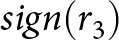 $sign(r_3)$. Abrupt direction shifts are frequently seen in natural phenomena, such as fish schools or flocks of birds. A “craziness” component, represented by a craziness variable in the model, is included to account for these unpredictable behaviors [Reference Ram, Mandal, Kar and Ghosal27]. The proposed technique consists of a crazy operator to preserve the diversity of particles. Using this operator, a preset probability is assigned to each particle exhibiting crazy behavior. Consequently, the particle’s velocity passes through a crazing process before updating its location. The particle’s motion becomes somewhat unpredictable or random due to this process. It is provided by this avoids early convergence and encourages exploration across the solution space. As shown in (13), the modified velocity of particles [Reference Sahoo and Mandal28, Reference Abualigah, Al Turk, Ikotun, Zitar, Alsoud, Khodadadi, Hussien and Jia29].
 \begin{equation}
V_i^{(k + 1)} = V_i^{(k + 1)} + P(r_4 ) \times sign(r_4 ) \times v^{Craziness}
\end{equation}
In this case,  $r_4$ is a consistently chosen random parameter from the interval [0, 1]. The variable representing insanity and craziness is randomly selected from an evenly distributed distribution falling between [
 $v_min$,
 $v_max$]. Figure 2 represents the working procedure or flow chart of the CRPSO. Furthermore, the definitions of
 $
P(r_4 )$ and
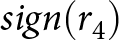 $sign(r_4)$ are as follows:
 \begin{equation}
P(r_4) =
\begin{cases}
1, & r_4 \gt P_{cr} \\
0, & r_4 \leq P_{cr}
\end{cases}
\end{equation}
 \begin{equation}
\text{sign}(r_4) =
\begin{cases}
1, & r_4 \lt 0.5 \\
-1, & r_4 \geq 0.5
\end{cases}
\end{equation}
CRPSO algorithm Flow chart.

Where  $P_{cr}$ stands for a preset probability of insanity.
Table 1 lists the parameters and values used for the CRPSO procedures. When optimizing an antenna array using CRPSO, there is a maximum of 500 iteration cycles and a maximum population size of 120. The variety of optimization tasks for ECA designing problems is modeled as the minimization of maximum SLL.
CRPSO parameters and their descriptions

Simulation results and numerical analysis
The numerical results of several CCAA designs are explained in this section. The CCAA radiation pattern is considered, with the significant lobe pointing to  $0^{\circ} $. Four non-uniform CCAAs antenna array sets with elements of (6, 12, 18), (10, 16, 22), (14, 20, 26), and (18, 24, 30) are presumed to exist. CRPSO algorithm parameters are shown in Table 1. In the test case of antenna array set 1 with elements of (6, 12, 18), array set 2 (10, 16, 22), array set 3 (14, 20, 26), and array set 4 (18, 24, 30) with non-uniform CCAA, respectively, optimized feed current and inter-element spacing with decreased SLL and improved FNBW are covered below. It is evident from the simulation results that the CRPSO technique is more effective at solving problems with enhanced directivity, effective aperture, and beam area when applied to a wide range of PSO, NPSO, Jaya algorithm, and prior work.
Test case of antenna array set 1: antenna array set 1 with elements configured as (6, 12, 18)
In test scenario 1, non-uniform CAA elements have been considered using antenna array set 1. Excitation amplitude and inter-element spacing have been optimized with low SLL and enhanced FNBW using the PSO, Jaya, CRPSO, and NPSO approaches. Concerning SLL, Table 2 shows that CRPSO outperforms uniform, PSO, Jaya, NPSO, and the current work SLL by -33.43 dB with an FNBW of  $33.90^{\circ} $. It is possible to conclude that the CRPSO approach is more effective at obtaining low SLL, enhanced directivity, and FNBW after comparing these values with data that have already been published. Other CCAA parameters can be computed using these optimal values, as indicated in Table 3. The radiation pattern with the highest SLL reduction and enhanced FNBW employing PSO, Jaya, NPSO, and CRPSO is displayed in Figure 3. It is evident from Figure 3 that the CRPSO technique, in contrast to the PSO, Jaya and NPSO techniques, decreased the maximum SLL. Using the CRPSO approach, Figure 4 displays the ideal feeding current and inter-element spacing values for antenna array set 1. Also, the geometry of the outline array set 1 is shown in Figure 5.
Optimal radiation pattern of the non-uniform CCAA (set 1) obtained using the CRPSO technique.

Optimized element spacing and excitation parameters for non-uniform circular antenna array (set 1) using CRPSO.

Corresponding geometrical configuration of the non-uniform CCAA for antenna array set 1, including element positions and radius.

Comparison of CRPSO-attained results with other optimization techniques for antenna array performance (Test case: antenna array set 1, configuration: 6, 12, 18 elements)

Comparison of additional performance metrics using CRPSO and other optimization techniques for antenna array set 1 (configuration: 6, 12, 18 elements)

Table 3 presents a comparative analysis of various performance parameters obtained using the CRPSO and other optimization methods. The evaluation focuses on antenna array set 1, configured with 6, 12, and 18 elements. The comparison highlights key performance indicators, including aperture efficiency, beam coverage area, directivity (DIR), total effective aperture, total beam coverage area, radius (r), and circumference (C). These parameters are crucial for evaluating and optimizing antenna array performance in beamforming applications.
Test case of antenna array set 2: antenna array set 2 with elements configured as (10, 16, 22)
In test scenario 2, a non-uniform CCAA is considered using antenna array set 2. The excitation amplitude and inter-element spacing have been optimized to achieve lower SLLs and improved FNBW through PSO, Jaya, CRPSO, and NPSO approaches. As shown in Table 5, the CRPSO method surpasses uniform, PSO, Jaya, NPSO, and previous works, achieving an SLL reduction of  $-$36.55 dB with an FNBW of
 $38.60^{\circ}$. These findings suggest that the CRPSO technique is more effective in attaining reduced SLL, enhanced directivity, and improved FNBW than existing studies. Using these optimized values, other CCAA parameters, including aperture efficiency, beam coverage area, directivity (DIR), total effective aperture, total beam coverage area, radius (r), and circumference (C), are used. These parameters are crucial for evaluating and optimizing antenna array performance in beamforming applications. These are determined as listed in Table 4. Figure 6 illustrates the radiation pattern obtained using PSO, Jaya, NPSO, and CRPSO, highlighting that the CRPSO approach significantly reduces the maximum SLL compared to the other methods. Figure 7 presents the optimal excitation current and inter-element spacing values for a non-uniform CCAA configuration of antenna array set 2, while Figure 8 depicts the corresponding antenna array geometry.
Optimal radiation pattern of the non-uniform CCAA (set 2) obtained using the CRPSO technique.

Optimized element spacing and excitation parameters for non-uniform circular antenna array (set 2) using CRPSO.

Corresponding geometrical configuration of the non-uniform CCAA for antenna array set 2, including element positions and radius.

Comparison of additional performance metrics using CRPSO and other optimization techniques for antenna array set 2 (configuration: 10, 16, 22 elements)

Comparison of CRSPO attained results with other optimization techniques for antenna array performance (Test case: antenna array set 2, configuration: 10, 16, 22 elements)

Test case of antenna array set 3: antenna array set 3 with elements configured as (14, 20, 26)
In test scenario 3, non-uniform CCAA elements have been considered using antenna array set 3. Excitation amplitude and inter-element spacing have been optimized with low SLL and enhanced FNBW using the PSO, Jaya, CRPSO, and NPSO approaches. Concerning SLL, Table 6 shows that CRPSO outperforms uniform, PSO, Jaya, NPSO, and current works attained SLL by  $-$35.08 dB with an FNBW of
 $38.80^{\circ}$. It is possible to conclude that the CRPSO approach is more effective at obtaining low SLL, enhanced directivity, and FNBW after comparing these values with data that have already been published. Other CCAA parameters include aperture efficiency, beam coverage area, directivity (DIR), total effective aperture, total beam coverage area, radius (r), and circumference (C). These parameters are crucial for evaluating and optimizing antenna array performance in beamforming applications. These are determined as listed in Table 7. The radiation pattern with the highest SLL reduction and enhanced FNBW employing PSO, Jaya, NPSO, and CRPSO is displayed in Figure 9. It is evident from Figure 9 that the CRPSO technique, in contrast to the PSO, Jaya, and NPSO techniques, decreased the maximum SLL. Using the CRPSO approach, Figure 10 displays the ideal feeding current and inter-element spacing values for antenna array set 3. Also, the geometry of antenna array set 3 is shown in Figure 11.
Optimal radiation pattern of the non-uniform CCAA (set 3) obtained using the CRPSO technique.

Optimized element spacing and excitation parameters for non-uniform circular antenna array (set 3) using CRPSO.

Corresponding geometrical configuration of the non-uniform CCAA for antenna array set 3, including element positions and radius.

Comparison of CRPSO-attained results with other optimization techniques for antenna array performance (test case: antenna array set 3, configuration: 14, 20, 26 elements)

Comparison of additional performance metrics using CRPSO and other optimization techniques for antenna array set 3 (configuration: 14, 20, 26 elements)

Test case of antenna array set 4: antenna array set 4 with elements configured as (18, 24, 30)
In test scenario 4, non-uniform CCAA elements have been considered using antenna array set 4. Excitation amplitude and inter-element spacing have been optimized with low SLL and enhanced FNBW using the PSO, Jaya, CRPSO, and NPSO approaches. Concerning SLL, Table 8 shows that CRPSO outperforms uniform, PSO, Jaya, NPSO, and current works by  $-$37.49 dB with an FNBW of
 $37.10^{\circ} $. It is possible to conclude that the CRPSO approach is more effective at obtaining low SLL, enhanced directivity, and FNBW after comparing these values with data that have already been published. Other CCAA parameters include aperture efficiency, beam coverage area, directivity (DIR), total effective aperture, total beam coverage area, radius (r), and circumference (C). These parameters are crucial for evaluating and optimizing antenna array performance in beamforming applications. These are determined as listed in Table 9. The radiation pattern with the highest SLL reduction and enhanced FNBW employing PSO, Jaya, NPSO, and CRPSO is displayed in Figure 12. It is evident from Figure 12 that the CRPSO technique, in contrast to the PSO, Jaya, and NPSO techniques, decreased the maximum SLL. Using the CRPSO approach, Figure 13 displays the ideal feeding current and inter-element spacing values for antenna array set 4. Also, the geometry of antenna array set 4 is shown in Figure 14. Table 10 presents the performance analysis of various non-uniform CCAA configurations using three optimization techniques to evaluate their effectiveness in antenna array synthesis. Meanwhile, Table 11 provides a comparative study assessing the improvements achieved by the proposed CRPSO algorithm over existing works. The analysis in Table 10 focuses on identifying overall performance trends among different optimization techniques, whereas Table 11 highlights the advantages of CRPSO in achieving superior results. These evaluations offer valuable insights into the optimal design and implementation of non-uniform CCAA configurations, contributing to enhanced performance in wireless communication systems.
Optimal radiation pattern of the non-uniform CCAA (set 4) obtained using the CRPSO technique.

Optimized element spacing and excitation parameters for non-uniform circular antenna array (set 4) using CRPSO.

Corresponding geometrical configuration of the non-uniform CCAA for antenna array set 4, including element positions and radius.

Comparison of CRPSO-attained results with other optimization techniques for antenna array performance (test case: antenna array set 4, configuration: 18, 24, 30 elements)

Comparison of additional performance metrics using CRPSO and other optimization techniques for antenna array set 4 (configuration: 18, 24, 30 elements)

Comparison and performance analysis of various non-uniform CCAA configurations using three distinct optimization techniques

Comparison of the performance of various non-uniform CCAA configurations using the proposed CRPSO algorithm with existing works

NR = not reported.
Implementation of the synthesized CCAA using HFSS
In this section, to explain about the synthesized CCAA using HFSS simulation software, we find the S-parameters, radiation pattern, full wave simulation, and scanned images of CCAA. The following are the dimensions, which are used in the design: length of substrate  $L_s = 60mm$, width of the substrate is
 $W_s = 60mm
$, length of the patch is
 $L_p = 28.2mm$, width of the patch is
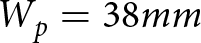 $W_p = 38mm$, length of the feed is
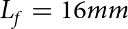 $L_f = 16mm$, width of the feed is
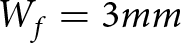 $W_f = 3mm$, length of the line-inset is
 $L_{inset} = 7.4mm$, width of the insert is
 $W_{inset} = 1mm$, and height of the substrate is
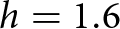 $h=1.6$.
From Figure 15, it is clear that the unit cell of rectangular patch with an operating frequency is 2.4GHz. Figure 16 represents the design of CCAA with non-uniform element spacings by using HFSS software; the inner ring consists of 6 elements, the middle ring consists of 12, the and outermost ring has 18 elements, total there are 36 elements used to design the non-uniform CCAA with different radii. Figure 17 depicts the S-parameters of our proposed structure; the designed antenna resonates at a frequency of 2.4GHz in full-wave simulation by using HFSS. Figure 18 describes the radiation patterns of our proposed antenna and it is plotted at 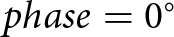 $phase = 0^{\circ}$ and
 $phase = 90^{\circ}$, the main lobe at
 $0^{\circ}$. Figure 19 explains about the radiation pattern of CCAA with uniform excitation amplitude; it is generated by using HFSS software scanned patterns in the design examples. Figure 20 explains about the radiation pattern of CCAA with non-uniform excitation amplitude; it is generated by using HFSS software scanned patterns in the design examples.
Unit cell rectangular patch.

Non-uniform CCAA structure.

S-parameters.

Radiation pattern polar plot.

Radiation pattern with uniform excitation amplitudes of CCAA.

Optimized radiation pattern of CCAA with non-uniform excitation amplitudes.

Conclusion
CCAAs often exhibit relatively high SLLs, which may be undesirable for many applications. Elevated SLLs can lead to increased interference and reduced ability to differentiate between desired and unwanted signals. Additionally, the concentric circular configuration of CCAAs presents design and optimization challenges compared to linear arrays, making it more difficult to control SLLs and beam shapes precisely. This study uses meta-heuristic optimization techniques to explore an innovative approach to antenna array design. Various algorithms, including PSO, Jaya, NPSO, and CRPSO, have been employed to determine the optimal feeding current and inter-element spacing. The objective is to achieve ultra-low SLL and enhanced FNBW. Among the techniques observed, CRPSO demonstrated superior performance across multiple design scenarios. Four different array configurations were examined: array set 1 (6, 12, 18 elements), array set 2 (10, 16, 22 elements), array set 3 (14, 20, 26 elements), and array set 4 (18, 24, 30 elements). In all cases, CRPSO achieved significant SLL reduction and improved FNBW. Furthermore, it facilitated maximum directivity in the antenna arrays. Despite the potential limitations of CCAA designs, such as reduced aperture efficiency compared to other configurations, the study recorded the highest effective aperture for a half-wave dipole antenna array under test conditions. Additionally, the maximum beam coverage area of the antenna array is summarized in a comparative table, where CRPSO outperformed the other methods. Also, compared with existing works, it is clear that CRPSO achieved superior SLL reduction.
Acknowledgements
The authors would like to express their sincere gratitude to the authorities of NITW for providing the necessary facilities to conduct this research. They also wish to thank the editors and anonymous reviewers for their valuable and constructive feedback.
Competing interests
The authors declare that they have no competing interests.

Nageswa Rao Thadikamalla earned his B.Tech. in Electronics and Communication Engineering from Kakatiya University, Warangal, India (2004), and his M.Tech. from IIT Kharagpur, India (2008). He earned his Ph.D. from the National Institute of Technology, Warangal (2025). He is currently working as an Assistant Professor in the School of Engineering, Department of ECE, Anurag University Hyderabad. He has 13 years of teaching experience. His research specializing in array antenna design using evolutionary computing techniques and smart antennas and time modulated antenna array.

Prakasa Rao Amara received his B.Tech. in Electronics and Communication Engineering from Nagarjuna University, A.P., India (1994), and an M.Tech. from PEC-Pondicherry, India (1998). He earned his Ph.D. from the National Institute of Technology, Warangal, India. With 24+ years of teaching experience, he is an Associate Professor at NIT Warangal, specializing in signal processing, smart antennas, and optimization, with a focus on adaptive beamforming of smart antenna arrays.



