


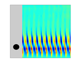

1. Introduction
Nuclear fusion is a good selection for energy production in the future due to its several potential advantages including high energy density, no greenhouse gas emissions and so on. While these advantages are compelling, significant scientific and engineering challenges have yet to be solved, which impede the economical production of fusion energy. The International Thermonuclear Experimental Reactor (ITER) has been designed to demonstrate the feasibility of nuclear fusion. Among the components in a fusion reactor such as the tokamak reactor, a kind of liquid metal blanket is selected due to the advantages of heat transfer and tritium breeding capabilities (Abdou et al. Reference Abdou, Morley, Smolentsev, Ying, Malang, Rowcliffe and Ulrickson2015). However, the existence of strong magnetic fields and high temperature gradients introduces challenges such as Lorentz and buoyancy forces, which must be carefully managed in the design of the liquid metal blanket to ensure high efficiency in heat and mass transfer (Smolentsev et al. Reference Smolentsev, Morley, Abdou and Malang2015; Mistrangelo et al. Reference Mistrangelo, Bühler, Alberghi, Bassini, Candido, Courtessole, Tassone, Urgorri and Zikanov2021; Smolentsev Reference Smolentsev2023). Until now, previous studies have proved that the adoption of vortex generators such as ribs, fins, grooved surfaces and obstacles in the flow channel can improve the heat transfer efficiency (Cassells, Hussam & Sheard Reference Cassells, Hussam and Sheard2016; Hussam et al. Reference Hussam, Hamid, Ng and Sheard2018; Kusumi et al. Reference Kusumi, Kunugi, Yokomine, Kawara, Wu, Sagara and Tanaka2019). A circular cylinder in proximity to a wall, as a traditional method of vortex promotion, generates quasi-two-dimensional (Q2-D) vortices under the magnetic field, effectively improving convection heat transfer (Moreau Reference Moreau1990; Husssam, Thompson & Sheard Reference Hussam, Thompson and Sheard2011; Hussam & Sheard Reference Hussam and Sheard2013). Studying the dynamic characteristics of magnetohydrodynamics (MHD) flow around an obstacle is highly beneficial for understanding heat transfer enhancement mechanisms.
The Lorentz force, induced by the liquid metal flow through a magnetic field, alters the dynamic characteristics of the Kármán vortex street. A strong magnetic field introduces a Q2-D flow state, as outlined in the Sommeria & Moreau (Reference Sommeria and Moreau1982) ‘SM82 model’. This model suggests that perturbations along the magnetic field such as turbulence and vortices, exhibit strong anisotropy due to the Lorentz force. The MHD flow around a cylinder under an axial magnetic field has been extensively researched in recent decades (e.g. Andreev & Kolesnikov Reference Andreev and Kolesnikov1998; Mück et al. Reference Mück, Günther, Müller and Bühler2000; Frank, Barleon & Müller Reference Frank, Barleon and Müller2001; Dousset & Pothérat Reference Dousset and Pothérat2008; Dousset & Pothérat Reference Dousset and Pothérat2012; Kanaris et al. Reference Kanaris, Albets, Grigoriadis and Kassinos2013; Rhoads, Edlund & Ji Reference Rhoads, Edlund and Ji2014; Chatterjee & Gupta Reference Chatterjee and Gupta2015; Hamid et al. Reference Hamid, Hussam, Pothérat and Sheard2015). The presence of an axial magnetic field serves to delay the onset of flow separation and vortex shedding, thereby contributing to a markedly increased critical Reynolds number (Recr) compared with that observed in hydrodynamic flows. As a result, Recr for vortex shedding in MHD flow maintains a linear relationship with the Hartmann number (Ha) (Recr/Ha ≈ 0.47, see Frank et al. Reference Frank, Barleon and Müller2001), quantifying the magnetic field strength. Moreover, Mück et al. (Reference Mück, Günther, Müller and Bühler2000) pointed out that the Kármán vortex street transitions from three-dimensional to Q2-D columnar vortices (also illustrated in Davidson Reference Davidson1997; Müller & Bühler Reference Müller and Bühler2001) when the interaction parameter N is greater than 1. Rhoads et al. (Reference Rhoads, Edlund and Ji2014) experimentally observed Kármán vortex street using electrical potential probes for 0 < N < 2.
Concerning the fluid around a circular cylinder near a wall, a substantial body of research has been conducted in the field of hydrodynamics. The findings indicate that the wall-proximity effect exerts a direct influence on the vortex dynamics characteristics and the flow transition after an obstacle (e.g. Bearman & Zdravkovich Reference Bearman and Zdravkovich1978; Kiya, Tamura & Arie Reference Kiya, Tamura and Arie1980; Zdravkovich Reference Zdravkovich1997; Zovatto & Pedrizzetti Reference Zovatto and Pedrizzetti2001; Dipankar & Sengupta Reference Dipankar and Sengupta2005; He et al. Reference He, Wang, Pan, Feng, Gao and Rinoshika2017; Jiang & Cheng Reference Jiang and Cheng2017; Thompson et al. Reference Thompson, Leweke and Hourigan2021; Zhou et al. Reference Zhou, Qiu, Li and Liu2021). It involves complex interactions among three shear layers: a boundary layer, a separating free shear layer and a wake street (Williamson Reference Williamson1996). The wall-proximity effect leads to separation delay, transitioning the wake region from unsteady to steady (see Bearman & Zdravkovich Reference Bearman and Zdravkovich1978; Zovatto & Pedrizzetti Reference Zovatto and Pedrizzetti2001). The aforementioned delayed separation indicates that the wall-proximity effect suppresses the instability observed in the wake street. Additionally, He et al. (Reference He, Wang, Pan, Feng, Gao and Rinoshika2017) noted that secondary vortex shedding from the wall shear layer, induced by an inverse pressure gradient, pushes the vortex street away from the wall. These secondary vortices significantly influence the wake trajectory and vortex intensity, leading to asymmetric velocity fluctuations.
However, to the authors’ knowledge, studies on MHD flow around a cylinder with the wall-proximity effect are rare, with only some Q2-D numerical studies focusing on heat transfer (Hussam et al. Reference Hussam, Thompson and Sheard2011; Hussam & Sheard Reference Hussam and Sheard2013). The three-dimensional effects, such as the Shercliff layer effect and the additional Joule dissipation caused by three-dimensional effects, have often been neglected in Q2-D simulations (e.g. Dousset & Pothérat Reference Dousset and Pothérat2008) and in some experiments (e.g. Belyaev et al. Reference Belyaev, Mironov, Luchinkin, Listratov, Kolesnikov, Kransov, Zikanov and Molokov2022), which, however, exhibit a significant effect on vortex shedding in this work. The three-dimensional (3-D) effects on the duct flow have been discussed in previous research by 3-D simulation (Mück et al. Reference Mück, Günther, Müller and Bühler2000; Pothérat Reference Pothérat2007; Cassells et al. Reference Cassells, Vo, Pothérat and Sheard2019). An experimental study is necessary to examine the strong 3-D effect, especially the wall-proximity effect on the MHD vortex street, which is the main purpose of the present study.
Several numerical studies for MHD flow around a cylinder with the wall-proximity effect have been conducted to enhance heat transfer (Hussam et al. Reference Hussam, Thompson and Sheard2011; Hussam & Sheard Reference Hussam and Sheard2013). Using Q2-D models, these studies focused on the influence of the blockage ratio and the gap ratio (G/d, defined as the ratio of the distance G from the bottom edge of the cylinder to the cylinder's diameter d) on heat transfer rather than the MHD effect. Hussam & Sheard (Reference Hussam and Sheard2013) noted that large blockage ratio (β, defined as the ratio of the cylinder's diameter d to the channel height H) improves heat transfer but at a great cost of pressure drop. In addition, a small blockage ratio (β = 0.1) with the effect of placing a circular cylinder close to the wall (G/d ≈ 1) optimizes heat transfer with a small pressure drop in a Q2-D simulation, leading to high energy efficiency. Hussam et al. (Reference Hussam, Thompson and Sheard2011) investigated the impact of the wall-proximity effect on heat transfer, with insufficient analysis of the vortex-shedding regime. In addition, the combined influence of the magnetic field and the gap ratio on the vortex-shedding regimes requires further detailed examination. Therefore, this study explores how the wall-proximity effect (G/d) influences the vortex shedding under various magnetic fields.
Furthermore, there is a lack of exploration into the variation of the Strouhal number (St) and the understanding of the flow regime under MHD conditions. Kolesnikov & Tsinober (Reference Kolesnikov and Tsinober1976) and Andreev & Kolesnikov (Reference Andreev and Kolesnikov1998) observed an increase in shedding frequency with an increase of Ha in their experiments. Moreover, they found that minor velocity fluctuations were observed within the shear layer of the cylinder, while significant velocity fluctuations were observed 1.5d downstream of the cylinder using electrical potential probes. They attributed this phenomenon to the oscillations of the shear layers stretched by the magnetic field at the rear of the cylinder. The numerical simulation in Hussam, Thompson & Sheard (Reference Hussam, Thompson and Sheard2012) with a small disturbance in the incoming flow confirmed this phenomenon.
The phenomenon of St increasing with the augmentation of the magnetic field was also observed in other research. Mück et al. (Reference Mück, Günther, Müller and Bühler2000) attributed the increase in the shedding frequency to the augmentation of the magnetic field to a square cylinder rather than a circular one. Dousset & Pothérat (Reference Dousset and Pothérat2008) and Hussam et al. (Reference Hussam, Thompson and Sheard2011) provided the evolution of St against Re for different Hartmann numbers (Ha). At a value of Re of approximately 3800, there was a decrease in the shedding frequency followed by an increase with the strengthening of the magnetic field. However, the authors did not offer any further discussion. Chatterjee & Gupta (Reference Chatterjee and Gupta2015) also observed the trend of St increasing with Ha, attributing this to the secondary vortices generated by the instability of the wall boundary layer. Nevertheless, previous researchers have been unable to reach a consensus on the mechanism by which the saturation parameter increases with the strength of the magnetic field.
In light of the latest research findings, previous researchers have identified different flow regimes under varying magnetic field conditions, except for a stable state when the Hartmann number (Ha) is sufficiently high or the Reynolds number (Re) is too low. Mück et al. (Reference Mück, Günther, Müller and Bühler2000) identified two flow regimes with β = 0.1: one dominated by inertial forces under a weak magnetic field, similar to the Kármán vortex street in hydrodynamics, and another dominated by Lorentz forces under a strong magnetic field, where the vortex street becomes Q2-D columnar vortices due to Hartmann friction (Frank et al. Reference Frank, Barleon and Müller2001; Hussam et al. Reference Hussam, Thompson and Sheard2011). Dousset & Pothérat (Reference Dousset and Pothérat2008) using the SM82 model obtained two vortex-shedding regimes (Chatterjee & Gupta Reference Chatterjee and Gupta2015): one with only vortex streets and another with interactions between vortex streets and secondary vortices, shedding from the Shercliff layers because of Kelvin–Helmholtz (K-H) instability (with β = 0.25). In this study, the results indicate that there are three distinct unsteady stages in the trend of St against the Hartmann friction parameter (Ha/Re), which suggests that there is still insufficient understanding of the variation of St and the flow regimes under MHD conditions. Furthermore, it is essential to investigate the impact of wall proximity on the vortex street under varying Re and Ha conditions. The objective of this study is twofold: firstly, to elucidate the mechanism behind the increase in shedding frequency with the strengthening magnetic field; and secondly, to investigate the wall-proximity effect on vortex dynamic characteristics.
The remainder of this paper is organized as follows: § 2 presents the Navier–Stokes equation for the MHD effect and the SM82 model. Section 3 details the experimental arrangement, measurement methods and verifications. Section 4 provides a detailed discussion of the main results. Section 5 summarizes the conclusions.
2. Basic equations with Lorentz force effect
2.1. Three-dimensional Navier–Stokes equations for MHD
The magnetic Reynolds number (Rem), which characterizes the relative effects of induction of a magnetic field to the magnetic diffusion, is defined as Rem = μσU 0a, where μ represents the magnetic permeability, σ denotes the electrical conductivity, U 0 stands for the mean flow velocity and a is the channel width. The values of these parameters are provided in table 1. The value of  $R{e_m}\sim O({10^{ - 3}})$ in this work is significantly less than 1, so the induced magnetic field is negligible but not the induced currents (Pan, Zhang & Ni Reference Pan, Zhang and Ni2019; Zhang et al. Reference Zhang, Yang, Ni, Zhang and Yu2023). The conservation of mass, non-dimensional momentum, charge and Ohm's law for incompressible and conductive fluids like liquid metals are, respectively,
 \begin{gather}\boldsymbol{\nabla }\boldsymbol{\cdot }\boldsymbol{u} = 0,\end{gather}
 \begin{gather}\frac{{\partial \boldsymbol{u}}}{{\partial t}} + (\boldsymbol{u}\boldsymbol{\cdot }\boldsymbol{\nabla })\boldsymbol{u} ={-} \boldsymbol{\nabla }p + \frac{1}{{Re}}\mathrm{\Delta }\boldsymbol{u} + N(\, \boldsymbol{j} \times \boldsymbol{B}),\end{gather}
 \begin{gather}\boldsymbol{\nabla }\boldsymbol{\cdot }\boldsymbol{j} = 0,\end{gather}
 \begin{gather}\boldsymbol{j} ={-} \boldsymbol{\nabla }\varPhi + \boldsymbol{u} \times \boldsymbol{B},\end{gather}
where p denotes the pressure, ρ the fluid mass density,  $\boldsymbol{B}$ the magnetic field,
 $\boldsymbol{u}$ the velocity vector,
 $\varPhi$ the electrical potential and v its kinematic viscosity. The term
 $N(\, \boldsymbol{j} \times \boldsymbol{B})$ represents the Lorentz force. The ratio of electromagnetic forces and viscous forces can be expressed as the interaction parameter N (where
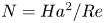 $N = H{a^2}/Re$). The interaction between the induced currents and the magnetic field generates Lorentz forces that tend to damp velocity variations along the streamlines (Sommeria & Moreau Reference Sommeria and Moreau1982).
Physical and non-dimensional parameters in the experiments.

2.2. The SM82 model under a strong magnetic field
In MHD channel flow with insulated walls, the boundary layer perpendicular to the direction of the magnetic field is called the Hartmann layer (the Hartmann layer's thickness  ${\delta _H}\sim H{a^{ - 1}})$, while the boundary layer parallel to the direction of the magnetic field is referred to as the Shercliff layer (the Shercliff layer's thickness
 ${\delta _S}\sim H{a^{ - 0.5}}$, Hunt & Ludford Reference Hunt and Ludford1968). When the magnetic field is sufficiently strong, the induced currents pass entirely through the boundary layers. Meanwhile, the velocity gradient in the core region along the direction of the magnetic field equals zero, while the velocity gradient only exists in the boundary layers. Therefore, the flow in the core region is two-dimensional, and referred to as Q2-D flow (Moreau Reference Moreau1990). As the velocity gradient along the direction of the magnetic field approaches zero (∂u/∂y = 0), (2.1) and (2.2) through (2.4) can be simplified to the following form:
 \begin{gather}\boldsymbol{\nabla }\boldsymbol{\cdot }{\boldsymbol{u}_ \bot } = 0,\end{gather}
 \begin{gather}\frac{{\partial {\boldsymbol{u}_ \bot }}}{{\partial t}} ={-} ({\boldsymbol{u}_ \bot }\boldsymbol{\cdot }{\nabla _ \bot }){\boldsymbol{u}_ \bot } - {\nabla _ \bot }{p_ \bot } + \frac{1}{{Re}}\nabla _ \bot ^2{\boldsymbol{u}_ \bot } - 2\frac{{{d^2}}}{{{a^2}}}\frac{{Ha}}{{Re}}{\boldsymbol{u}_ \bot }.\end{gather}
By taking d,  $\rho U_0^2$ and d/U 0 as the typical length, pressure and time, respectively, the Lorentz force is simplified to a linear friction term, as shown in (2.5) and (2.6). The linear Hartmann friction parameter (Ha/Re) is also called the Hartmann damping term, a dominant parameter for vortex shedding under a magnetic field. In addition, the linear friction parameter Ha/Re caused by the Hartmann layer is considered as the effective ratio of Lorentz forces to inertial forces (see Sreenivasan & Alboussière Reference Sreenivasan and Alboussière2002; Chatterjee & Gupta Reference Chatterjee and Gupta2015).
The fundamental principle behind using electrical potential probes to measure velocity is based on Ohm's law  $\boldsymbol{j} = \sigma (\boldsymbol{E} + \boldsymbol{u} \times \boldsymbol{B})$, where
 $\boldsymbol{E}$ denotes the electric field. This law relates the electric potential measured by the probes to the flow velocity, enabling the determination of fluid speed through the analysis of electrical properties within the flow field.
3. Experimental set-up and validation
3.1. Configuration of the liquid metal loop
Experiments were conducted using a liquid metal loop at the University of Chinese Academy of Sciences (UCAS), known as the Magneto-Thermo-Hydrodynamic (MaTHE) loop. The experiments were performed in an insulated channel (see figure 1a), oriented horizontally within a uniform magnetic field. The field was created by an electromagnet with overall pole dimensions of 1200 mm length and 320 mm height, in a gap of 80 mm. The electromagnet can generate a magnetic field (B 0) of up to 2.0 Tesla (T), with inhomogeneity maintained below 5 % to ensure uniformity. Fluid motion within the channel was driven by an electromagnetic pump (EMP60-GA), with fluctuations ranging from 4 % (when Re = 180) to 1 % (when Re = 810) during the experiments.
(a) Configuration of the test section and the x-distribution component of the imposed magnetic field B 0. (b) Schematic diagram of the experimental set-up.

The metallic fluid flows through a pipeline into a heat exchanger, where the temperature is regulated to 22 ± 0.5 °C. Subsequently, it passes through an electromagnetic flowmeter (Emerson 8711 series), which upholds an accuracy class of 0.2 with a volumetric flow rate range from 0 to 0.8 m3 h−1. Finally, liquid metal fluid flows into the inlet of the test section.
To further refine the flow quality entering the measurement section, two 3D-printed honeycomb structures were incorporated upstream of the inlet. These honeycombs played a pivotal role in enhancing the uniformity of the flow entering the channel, effectively mitigating large-scale turbulence and flow inconsistencies at the entry cross-section. The upstream honeycomb was situated at the entry of the magnetic field to minimize the potential gradient effect, as supported by Belyaev et al. (Reference Belyaev, Sardov, Melnikov and Frick2021). The liquid metal flowed through the contraction section, honeycomb section, fully developed section and finally flowed around a cylinder. The cylinder, with its axis parallel to the magnetic field and capable of modifying its distance from the bottom wall, was positioned more than 650 mm (exceeding 108d) downstream from the flow inlet. This distance ensures the flow is fully developed before encountering the cylinder.
Additional aspects related to the experimental set-up, such as configuration details, measurement techniques and verification procedures, are elaborated in the following subsections of § 3.
3.2. Parameters and variables in the experiments
All the walls and the cylinder were made of acrylic to maintain insulated boundary conditions. The channel, with a width (a) of 40 mm and a half-height (b) of 30 mm (see figure 1b), yields a blockage ratio (β) of approximately 0.1 and an aspect ratio (α) of 6.67.
Galinstan, a eutectic alloy comprising gallium (Ga), indium (In) and tin (Sn) in the ratio of 67 %, 20.5 % and 12.5 % respectively, served as the working fluid. The physical properties of Ga67In20.5Sn12.5, including density (ρ), kinematic viscosity (ν) and electrical conductivity (σ) at an operational temperature of 22 ± 0.5 °C are listed in table 1 (refer to Morley et al. Reference Morley, Burris, Cadwallader and Nornberg2008).
The flow rate varied from 0.078 to 0.350 m3 h−1, achieving a mean velocity (U 0) ranging from 0.0090 to 0.0404 m s−1. These velocities correspond to Reynolds numbers (Red, also Re in this work) spanning from 180 to 810 based on the cylinder's diameter, and Reynolds numbers (Rech) ranging from 1200 to 5400 based on the channel height. The magnetic field was varied from 0.05 to 1.0 T, allowing exploration of Had from approximately 12.1 to 242.4 and Hach (also Ha in this work) from 81 to 1616. The experiments were conducted with six gap ratios G/d ranging from 0.5 to 3.0 to examine the wall-proximity effect. For each Reynolds number (Rech) and Hartmann number (Hach), the interaction parameter (N) ranged from 1.2 to 2.2 × 10³, all of which are greater than one, fulfilling the prerequisites of the SM82 model by Sommeria & Moreau (Reference Sommeria and Moreau1982). This adherence confirms the Q2-D nature of the flow under the influence of the magnetic field. Other non-dimensional parameters, including the Strouhal number (St) and set-up characteristics, are also provided in table 1.
3.3. Velocity measurements by electrical potential probes
To accurately capture fluid flow under a magnetic field, wall electrical potential probes (Wall-EPV, see figure 1) were employed to measure velocity through potential differences (Eckert, Cramer & Gerbeth Reference Eckert, Cramer and Gerbeth2007). As depicted in figure 2, the probes, positioned at x = 7.5d downstream from the cylinder, were inserted into specifically designated slots on one side of the channel wall. The placement, at 7.5d downstream from the cylinder, is a proper position for capturing the evolved flow patterns, such as the Kármán vortex street (Frank et al. Reference Frank, Barleon and Müller2001; Rhoads et al. Reference Rhoads, Edlund and Ji2014; Zhang et al. Reference Zhang, Yang, Ni, Zhang and Yu2023).
Arrangement and detailed configuration of the wall electrical potential probes. (a) Arrangement of the wall electrical potential probes and (b) photo of the electrical potential probes.

In the presence of a sufficiently strong magnetic field, the core flow exhibits Q2-D characteristics (referred to as the SM82 model), maintaining nearly constant potential along the magnetic field direction (see Sommeria & Moreau Reference Sommeria and Moreau1982; Pothérat & Klein Reference Pothérat and Klein2014). However, Mück et al. (Reference Mück, Günther, Müller and Bühler2000) noted that the potential distribution is not strictly two-dimensional under a strong magnetic field. The potential isolines along the direction of the magnetic field exhibit a certain curvature. The potential differences measured by non-intrusive wall probes may fall below the measurement accuracy. In this case, non-intrusive potential probes can no longer detect existing cigar-like vortices (Mück et al. Reference Mück, Günther, Müller and Bühler2000). Therefore, the probes were immersed 2 mm into the fluid to measure the electrical potential difference of the core flow, thrusting across the thickness of the Shercliff layer (δS) (see Sommeria & Moreau Reference Sommeria and Moreau1982; Cassells et al. Reference Cassells, Vo, Pothérat and Sheard2019). Simultaneously, this approach prevented the adhesion of oxides to the tip of probes and ensured the rigidity of the potential probes. The effectiveness of wall electrical probes has been verified by prior studies (e.g. Burr et al. Reference Burr, Barleon, Müller and Tsinober2000; Frank et al. Reference Frank, Barleon and Müller2001; Messadek & Moreau Reference Messadek and Moreau2002; Sreenivasan & Alboussière Reference Sreenivasan and Alboussière2002; Mistrangelo & Bühler Reference Mistrangelo and Bühler2018; Bühler, Mistrangelo & Brinkmann Reference Bühler, Mistrangelo and Brinkmann2020).
During the experiments, a data acquisition system comprising 58 voltage channels was sampled simultaneously at a frequency of 250 Hz over a duration of 300 seconds. The sampling frequency was designed to cover the vortex-shedding frequency range of approximately 1.5 Hz, ensuring multiple shedding cycles were captured.
To eliminate potential noise, specifically the 50 Hz electrical noise, a low-pass filter with a 45 Hz cutoff was implemented. Subsequently, signal quality was refined by subtracting the average noise level, measured under identical magnetic conditions but in the absence of flow. The resultant signals, with a noise floor below 2 microvolts and signal strength exceeding 10 microvolts, yielded a signal-to-noise ratio exceeding 5, indicating high-quality measurements.
Following the principles outlined in the SM82 model, velocity measurements are derived from the potential differences recorded by the probes. Previous studies have examined errors stemming from the internal currents on the measured potential gradient, suggesting negligible impact at  $N \gg 1$ and
 $Ha \gg 1$ (see Frank et al. Reference Frank, Barleon and Müller2001; Messadek & Moreau Reference Messadek and Moreau2002; Belyaev et al. Reference Belyaev, Mironov, Luchinkin, Listratov, Kolesnikov, Kransov, Zikanov and Molokov2022). During the experiments, the minimum Ha is 81 and the minimum N is 1.21, satisfying the assumptions proposed by the SM82 model. The formula for velocity calculation are as follows:
 \begin{gather}u(x,z) = \frac{{{\phi _{wall }}(x,z + \Delta z) - {\phi _{wall }}(x,z)}}{{{c_1}{B_0}\Delta z}},\end{gather}
 \begin{gather}w(x,z) ={-} \frac{{{\phi _{wall }}(x + \Delta x,z) - {\phi _{wall }}(x,z)}}{{{c_1}{B_0}\Delta x}},\end{gather}
where  ${\phi _{wall }}$ is the electric potential difference of two adjacent probes. The distances between the two adjacent probes in the x-direction and z-direction are
 $\mathrm{\Delta }x = 2\ \textrm{mm}$ and
 $\mathrm{\Delta }z = 2\ \textrm{mm}$, respectively. The coefficient
 ${c_1}$ depends on the condition of closing the induced currents. For Hartmann numbers greater than 200,
 ${c_1}$ approaches unity, aligning the probe-measured velocity with actual flow velocities (Belyaev et al. Reference Belyaev, Mironov, Luchinkin, Listratov, Kolesnikov, Kransov, Zikanov and Molokov2022). If Ha is not large enough,
 ${c_1}$ becomes greater than unity, resulting in a larger velocity than its actual value.
To illustrate the impact of upstream probes on downstream probes, the probe can be considered as cylinders with a diameter of 0.35 mm. The calculated Reynolds number (Reprobe) ranges from 10.5 to 47.25. Under these Reprobe conditions, the flow state of MHD flow around a circular cylinder remains stable with no vortex shedding. The length of the recirculation zone ranges from 0.175 to 1.05 mm (Dousset & Pothérat Reference Dousset and Pothérat2008), which is significantly smaller than the 2 mm distance between probes. Consequently, using a spatial resolution of 2 mm, the influence of upstream probes on downstream measurements is negligible.
3.4. Validation of measurement techniques
Comprehensive validation tests were conducted to ensure the accuracy and reliability of the present experimental results. For different G/d, Re and Ha, time-averaged velocities Ux and U 0, were determined by the electrical probes and the electromagnetic flowmeter, respectively. The normalized time-averaged velocity (Ux/U 0) and its error bars are plotted in figure 3(a). Under a strong magnetic field (Ha > 200), the errors in normalized velocity are less than 5 % and decrease with increasing Ha. However, for Ha < 200, the velocity calculated by electrical potential difference is larger than the actual velocity, with a maximum error of less than 20 %. This is related to the correction coefficient  ${c_1}$ being greater than 1, as induced by the non-negligible induced current (Belyaev et al. Reference Belyaev, Sardov, Melnikov and Frick2021).
(a) Time-averaged velocity calibration for different G/d, Re and Ha. (b) The correlation coefficient calculated by  ${u^{\prime}_z}$ fluctuation versus Ha at Re = 810 and G/d = 2.5, 3.0, 4.5.

To obtain correlation coefficients and assess the Q2-D or 3-D nature of the flow (see Pothérat & Klein Reference Pothérat and Klein2014), two probes at the same spatial coordinates (x 0, z 0) were installed on the opposite wall. The probes, extending 2 mm into the core flow across the Hartmann layer, are used to measure potential fluctuations and calculate vertical velocity fluctuations. The vertical velocity fluctuations  ${u^{\prime}_z}({x_0},{y_1},{z_0},{t_i})$ and
 ${u^{\prime}_z}({x_0},{y_2},{z_0},{t_i})$ are derived to calculate their cross-correlation coefficient (see Klein, Pothérat & Alferenok Reference Klein, Pothérat and Alferenok2009). The specific formula is as follows:
 \begin{gather}
R_{u^{\prime}_{z}}=\frac{\displaystyle\sum\limits_{i=1}^{n}({u^{\prime}_z}({x_0},{y_1},{z_0},{t_i})\times
{u^{\prime}_z}({x_0},{y_2},{z_0},{t_i}))}{\sqrt{\displaystyle\sum\limits_{i=1}^{n}({u^{\prime}_z}({x_0},{y_1},{z_0},{t_i}))^{2}
\displaystyle\sum\limits_{i=1}^{n}
({u^{\prime}_z}({x_0},{y_2},{z_0},{t_i}))^{2}}}
\end{gather}
where the coordinates of the vertical velocities are x 0 = 48 mm, y 1 = 2, y 2 = 38 mm and z 0 = 28 mm. The sampling number n equals to75 000.
It should be mentioned that the wake street keeps far from the probes when the cylinder is not near the probes. Therefore, the small gap ratios (G/d = 0.5–2.0) lead to weak velocity fluctuations in the two probes for the correlation coefficients, resulting in a low signal-to-noise ratio. Consequently, the correlation coefficient  ${R_{{u^{\prime}_z}}}$ is only calculated when the cylinder is positioned at G/d = 2.5, 3.0 and 4.5 (figure 3b).
The correlation coefficient  $({R_{{u^{\prime}_z}}})$ highlights the Q2-D character of the flow under varying magnetic intensities. As figure 3(b) reveals, the correlation sustainably increases with the magnetic field when Ha is smaller than 200. The low values of
 ${R_{{u^{\prime}_z}}}$ at small Ha are attributable to the insufficiently pronounced 2-D character of the shedding vortices. The correlation coefficient
 ${R_{{u^{\prime}_z}}}$ values increase to values above 0.8 for 200 < Ha < 800 (for Ha/Re ∼ 0.25–0.99), indicating a pronounced Q2-D nature of the flow within this range of Ha. However, for Ha greater than 800 (for Ha/Re
 $\gtrsim$ 1.0), there is a notable decrease in
 ${R_{{u^{\prime}_z}}}$ due to the increasing role of friction in a strong magnetic field within the Hartmann layers, the thickness ‘δH’ of which is proportional to Ha −1. This increase in friction leads to a rapid dissipation of vortices as they move downstream. Furthermore, we note also that the correlations decrease for the given G/d, starting from a value of Re/Ha of the order of unity, which determines the ratio of inertial forces to Hartmann friction forces. Therefore, at Re/Ha
 $\lesssim$ 1.0, there is precisely the predominance of friction forces.
Figure 4 presents critical Reynolds numbers (Recr) against Ha, aligning well with prior works by Frank et al. (Reference Frank, Barleon and Müller2001) and Hussam et al. (Reference Hussam, Thompson and Sheard2011). Frank et al. (Reference Frank, Barleon and Müller2001) obtained a critical vortex-shedding parameter (Recr/Ha) of around 0.47, whereas in this work, Recr/Ha is in the range of 0.56 ± 0.08. The slight difference may be attributed to the different aspect ratios, with α = 5 in Frank's study and α = 6.67 in this paper. Additionally, the critical shedding curve exhibits a strong linear relationship with Re/Ha, consistent with conclusions obtained by Frank et al. (Reference Frank, Barleon and Müller2001). However, notable discrepancies in Recr/Ha exist with the findings of Dousset & Pothérat (Reference Dousset and Pothérat2008) and Kanaris et al. (Reference Kanaris, Albets, Grigoriadis and Kassinos2013), which are attributed to different blockage ratios (β = 0.1 in this study, while they had β = 0.25, see Hussam, Thompson & Sheard Reference Hussam, Thompson and Sheard2012).
Critical Reynolds numbers (Recr) against Ha.

4. Results and discussion
Previous research in hydrodynamics indicates that flow around a circular cylinder in proximity to a wall induces secondary vortex shedding from the shear layer near the wall, leading to asymmetry in the velocity profile and the formation of a reverse Kármán vortex street (see Zovatto & Pedrizzetti Reference Zovatto and Pedrizzetti2001; He & Wang Reference He and Wang2015; Zhou et al. Reference Zhou, Qiu, Li and Liu2021). This section investigates the influence of the magnetic field and wall-proximity effect on the MHD flow state and the vortex-shedding regime. A Kármán vortex street, reverse Kármán vortex street and secondary vortices were observed through electrical potential probes. The approach for observing Kármán vortex streets is analogous to that of Rhoads et al. (Reference Rhoads, Edlund and Ji2014). Velocity fluctuations are contoured in both streamwise and vertical directions, whereas Rhoads et al. only plotted velocity fluctuations in the streamwise direction with small Ha (0 < N < 2). The variation in St should be particularly noteworthy, as it has not been thoroughly analysed until now. The following results examine the effect of wall proximity and the magnetic field on vortex shedding.
4.1. Impact of the magnetic field on flow regime with weak wall-proximity effect for G/d = 2.0
4.1.1. Flow regime for Re = 810
As depicted in figures 5 and 6, the contours of dimensional velocity fluctuations show negative values in blue and positive values in red. According to the classical theory of the Kármán vortex street (see Williamson Reference Williamson1996), vortices shedding from the upper surface of the cylinder follow a clockwise rotation, inducing positive velocity fluctuations on the upper side and negative velocity fluctuations on the lower side of these vortices. Conversely, vortices shedding from the lower surface of the cylinder exhibit a counterclockwise rotation, resulting in negative velocity fluctuations on the upper side and positive velocity fluctuations on the lower side. Similar conclusions can be drawn for velocity fluctuations on the left and right sides of the vortices. Therefore, the alternating pattern of positive and negative velocity fluctuations aligns with the Kármán vortex street.
Contour map of velocity fluctuations  ${u^{\prime}_x}$ with varying magnetic fields for G/d = 2.0 at x = 7.5d. Panels show (a) Ha = 81, Re/Ha = 10.0, (b) Ha = 323, Re/Ha = 2.50, (c) Ha = 646, Re/Ha = 1.24, (d) Ha = 969, Re/Ha = 0.84 and (e) Ha = 1131, Re/Ha = 0.72.

Contour maps of velocity fluctuations  ${u^{\prime}_z}$ with varying magnetic fields for G/d = 2.0 at x = 7.5d. Panels show (a) Ha = 81, Re/Ha = 10.0, (b) Ha = 323, Re/Ha = 2.50, (c) Ha = 646, Re/Ha = 1.24, (d) Ha = 969, Re/Ha = 0.84 and (e) Ha = 1131, Re/Ha = 0.72.

For 81 ≤ Ha ≤ 323 (see figures 5a,b and 6a,b), the intensity of the vortices rises with a stronger magnetic field. This enhancement is due to the augmented two-dimensionality of the vortices and a corresponding decrease in Joule dissipation. Consequently, the vortices become more regular, robust and coherent as the magnetic field increases. Enlarged fragments of the Kármán vortex street are depicted in figures 5(b*) and 6(b*).
For 323 ≤ Ha ≤ 646, an increase in magnetic field strength leads to reduced intensity (see figures 5b,c and 5b,c) and frequency of vortex shedding (see also figure 7b,c). This reduction is attributed to the enhanced influence of Hartmann friction, which affects both the formation of vortices immediately behind the cylinder and their propagation downstream to the measuring cross-section.
Spectra of  ${u^{\prime}_x}$ and
 ${u^{\prime}_z}$ corresponding to the point of maximum
 ${({u^{\prime}_z})_{rms}}$ velocity fluctuations (G/d = 2.0). Panels show (a) Ha = 81, Re/Ha = 10.0, (b) Ha = 323, Re/Ha = 2.50, (c) Ha = 646, Re/Ha = 1.24, (d) Ha = 969, Re/Ha = 0.84 and (e) Ha = 1131, Re/Ha = 0.72.

For 646 ≤ Ha ≤ 969 (see figures 5c,d and 6c,d), the amplitude of velocity fluctuations decreases with the rising magnetic field, which is attributed to the suppression of vortex shedding by the field behind the cylinder. At a certain distance from the cylinder, vortices arise due to K-H-type instability in the velocity shear region in the wake. Furthermore, the frequency of vortices noticeably increases, apparently due to the narrowing of the wake behind the cylinder.
For 969 < Ha ≤ 1131 (see figures 5d,e and 6d,e), the increasing magnetic field rapidly dissipates the vortex intensity. The oscillation of the wake is almost completely suppressed by a sufficiently strong magnetic field. The velocity fluctuations are nearly dissipated by Hartmann friction, with only slight and irregular vertical velocity fluctuations  ${u^{\prime}_z}$.
Consequently, for Ha ≥ 1131, periodic shedding is unobservable at x = 7.5d (figures 5e and 6e). Only weak transverse velocity fluctuations of an intermittent character are visible, and no prominent peak is observed in the spectrum (figure 7e).
The point with the maximum vertical velocity fluctuation  ${({u^{\prime}_z})_{rms}}$ is used for the power spectral density (PSD) analysis (figure 7). The peak points of the vertical component
 ${u^{\prime}_z}$ are located near the coordinate z = 15 mm, corresponding to the position of the cylinder axis (figure 8b). The two peak values of the streamwise component
 ${u^{\prime}_x}$ are located on both sides of this coordinate (figure 8a). This observation aligns with classical theories in vortex dynamics (Zdravkovich Reference Zdravkovich1997), predicting the distribution of velocity pulsation intensities in the wake of a vortex street. Both the fundamental shedding frequency and its corresponding harmonics are observed in the spectrum, resulting from the alternating shedding vortices and wake oscillations.
The r.m.s. of non-dimensional velocity fluctuations  ${({u^{\prime}_x})_{rms}}$ and
 ${({u^{\prime}_z})_{rms}}$ under different magnetic fields (G/d = 2.0, at x = 7.5d).

At Ha = 161 (figure 7a), the spectrum exhibits a power decay rate of −5/3, indicating that 3-D flow is prominent. As the magnetic field increases to Ha = 323 (figure 7b), the order of energy amplifies from 10−4 to 10−3, the shedding frequency slightly increases and the flow transitions to a Q2-D flow state with a decay rate approaching −3. With increasing magnetic field, the shedding frequency initially decreases and then increases (figure 7b–d). For Ha = 1131 (figure 7e), the slope of the decay rate approaches −3 but with no dominant peak for frequency, consistent with figures 5(e) and 6(e). The energy order falls from 10−3 to 10−7 as the magnetic field changes from Ha = 323 to Ha = 1131.
The variation in the intensity of velocity fluctuations across the transverse direction reflects the spanwise distance and strength of vortices. In figure 8, the root-mean-square (r.m.s.) of velocity is presented under various magnetic fields, showing a consistent trend with the energy of the vortices. For G/d = 2.0, the r.m.s. of velocity fluctuations increases with the magnetic field from Ha = 81 to 323. This increase of vortex intensity is related to the transition from 3-D flow to Q2-D flow, accompanied by the energy transport from small-scale vortices to large-scale vortices. However, further increment of the magnetic field for Ha > 323 results in a decrease in velocity fluctuations, which is due to the dissipation of the Hartmann friction. When B ≥ 0.7 T (Ha ≥ 1131), the r.m.s. of velocity fluctuations approaches a near-zero value, indicating that vortex shedding is completely suppressed or dissipated at x = 7.5d.
According to the theory of the vortex wake behind a cylinder, the centres of the wake street correspond to local maxima in the r.m.s. values of the vertical velocity fluctuations  ${u^{\prime}_z}$. As shown in figures 5 and 6, the vertical velocity fluctuations
 ${u^{\prime}_z}$ are predominantly concentrated in the height range of z = 9–21 mm (equivalent to 2d), while the amplitude of the velocity fluctuations rapidly decreases beyond this range. However, the influence of the streamwise velocity fluctuations extends over a greater range of z = 5–25 mm (approximately 3.3d), beyond which the velocity fluctuations decrease more slowly. Furthermore, the magnetic field not only dissipates the energy of the vortices but also narrows the vortex street (figure 6).
4.1.2. Vortex-shedding frequency and phase diagram for Re = 180–810
The relationship between the Strouhal number (St) and the ratio Re/Ha is depicted in figure 9(a). In weak magnetic fields, the trend of St changing to Re/Ha is similar to the relationship between St and Re in hydrodynamics. Under moderate magnetic fields, St increases with increasing flow rate and decreasing magnetic field for Re/Ha  $\gtrsim$ 1. However, St increases with Re/Ha under strong magnetic fields (Re/Ha
 $\lesssim$ 1).
(a) Relationship between St and Re/Ha. (b) Phase diagram (for G/d = 2.0).

The flow regimes are often defined by the fluctuations, spectra and frequency of the velocity. In this research, the regimes of vortex shedding are categorized into three different regimes based on the trend of St against Re/Ha, excluding the ‘stable state’ (see figure 9b), which are defined and analysed as follows:
(i) Regime I, for 0.56  $\lesssim$ Re/Ha
 $\lesssim$ 1.0 – ‘oscillations of attached vortices and wake shear layers’, dominated by the Lorentz force and Hartmann friction (for 808 < Ha < 1131, at Re = 810). In the regions Re/Ha
 $\lesssim$ 1.0, the frequency of vortex shedding increases with growing Ha. Notably, the order of vortex energy remains above 10−4 for Re/Ha
 $\gtrsim$ 1.0 (figure 7a–c), but it drops suddenly down during Re/Ha
 $\lesssim$ 1.0 (figure 7d,e). This change comes from the different vortex-shedding regimes. Although previous researchers (Andreev & Kolesnikov Reference Andreev and Kolesnikov1998; Frank et al. Reference Frank, Barleon and Müller2001; Dousset & Pothérat Reference Dousset and Pothérat2012) observed the nonlinear variations of the physical parameters against magnetic field strength, they did not attribute these phenomena to a new mode of vortex shedding.
Andreev & Kolesnikov (Reference Andreev and Kolesnikov1998) noted that the magnetic field delays the separation of vortices but does not suppress the instability of the extended shear layer, explaining the increase of vortex-shedding frequency in a narrowing wake with an increasing magnetic field. In this work, the contour maps show regular vortex shedding at x = 7.5d in this regime (figures 5d,e and 6d,e). The vortices shed from the oscillating shear layer due to the K-H instability. It can be confirmed that the parameter range for the existence of the shear layer oscillation is broad (Re ∼ 270–810, Ha ∼ 323–1131). With a sufficiently strong magnetic field (Ha >> Re), the wake vortex oscillation is completely suppressed, leaving two attached vortices at the rear of the cylinder with no vortex generation.
The primary difference between the vortex-shedding modes under strong and weak magnetic fields lies in the vortex generation mechanism. In regime I, as Ha increases, the flow around the cylinder experiences additional intensified dissipation mechanisms associated with Hartmann friction and Joule dissipation. These mechanisms broaden the range of the Re/Ha parameter values for transient processes compared with those without a magnetic field. At high Ha, the oscillations of the attached vortices and the wake occur. In this scenario, the vortex street is narrowed and the vortex intensity is significantly reduced. Vortex detachment occurs at the tail of the shear layer, and the pressure difference on both the upper and lower sides of the cylinder approaches zero. The shear layers are stretched, causing the recirculation length to extend up to 2d due to the negative velocity in the recirculation zone, which leads to a streamwise Lorentz force. The viscous force and Lorentz force balance each other within the stretched shear layer. The vortices are shed from the oscillating shear layers due to K-H instability (figures 6d and 6e), rather than pressure difference. Moreover, as Ha decreases, K-H-type shear instability develops along the wake with the formation of vortices at a certain distance from the cylinder. These vortices were detected by the measuring sensor at the distance of x = 7.5d. With a further decrease in Ha, the point of vortex formation moves closer to the cylinder, and when Re/Ha  $\lesssim$ 1.0, the vortices are shed directly by the cylinder (figure 9a).
(ii) Regime II, for 1.0  $\lesssim$ Re/Ha
 $\lesssim$ 2.50 – Q2-D vortex shedding’, characterized by a competition between Lorentz force and inertia force (for 323
 $\lesssim$ Ha
 $\lesssim$ 808, at Re = 810). For Re/Ha
 $\gtrsim$ 1.0, both the Strouhal number and vortex intensity increase with increasing Re/Ha. As the magnetic field decreases (resulting in an increase in Re/Ha), vortex detachment occurs on the cylinder's surface due to the combined action of pressure, viscous forces and Lorentz forces within the boundary layer. This detachment is primarily caused by a pressure differential that leads to the separation of the boundary layer. The vortices appear barrel-like (or cigar-like) in shape, as observed by Mück et al. (Reference Mück, Günther, Müller and Bühler2000). Additionally, the vortices maintain a column-like shape along the streamwise direction for a moderate magnetic field, perfectly satisfying the condition of the Q2-D model. Therefore, this vortex-shedding regime should be considered a Q2-D mode during the formation of Kármán street under a moderate magnetic field (figures 6b and 6c).
(iii) Regime III, for Re/Ha  $\gtrsim$ 2.50 – ‘transition of magnetohydrodynamic to hydrodynamic Kármán street’, dominated by the inertia force (for Ha ≤ 323, at Re = 810). In this regime, as Re/Ha increases, the inertia force tends to exceed the Lorentz force, resulting in the transition from Q2-D flow to 3-D flow. The coherent Q2-D columnar vortex breaks down into smaller 3-D vortices with increasing Re/Ha, and the effect of Joule dissipation becomes increasingly significant (figures 6a). Additionally, the frequency of vortex shedding exhibits a slight increase with rising Re. In this regime, the vortex-shedding frequency shows a non-monotonic variation, potentially analogous to transition modes observed in ordinary hydrodynamics. As noted by Williamson (Reference Williamson1996), the transformation of vortex-shedding modes results in energy transport, involving the transfer of energy from 2-D columnar vortex structures to 3-D vortex configurations, accompanied by the decrease of the correlation coefficient for Re/Ha
 $\gtrsim$ 2.04 (figure 3(b) for Ha < 400).
4.2. Impact of the magnetic field on flow regime with strong wall-proximity effect for G/d = 0.5
4.2.1. Flow regime for Re = 810
The wall-proximity effect for G/d = 0.5, compared with G/d = 2.0, leads to significant differences in vortex dynamics characteristics. At Ha = 81 (figures 10a and 11a), the trajectory of the vortex street exhibits slight vertical undulations with the vortex core oscillating near z = 10 mm (the centre of the cylinder is at z = 6 mm). The vortex structure appears irregular, with numerous small vortices present. These undulations and irregular shedding of vortices in the vortex street may be attributed to unsteady variations in the size of the recirculation region near the wall, which strongly affect the interaction and trajectory of the vortices. Additionally, the velocity fluctuations near the wall at G/d = 2.0 (figures 5 and 6) are significantly larger than those at G/d = 0.5 (figures 10 and 11). This observation further supports the presence of a strong interaction between the Kármán vortex street and the wall-proximity effect.
Contour maps of velocity fluctuations  ${u^{\prime}_x}$ with varying magnetic fields for G/d = 0.5 at x = 7.5d. Panels show (a) Ha = 81, Re/Ha = 10.0, (b) Ha = 323, Re/Ha = 2.50, (c) Ha = 646, Re/Ha = 1.24, (d) Ha = 969, Re/Ha = 0.84, (e) Ha = 1131, Re/Ha = 0.72 and (f) Ha = 1292, Re/Ha = 0.64.

Contour maps of velocity fluctuations  ${u^{\prime}_z}$ with varying magnetic field for G/d = 0.5 at x = 7.5d. Panels show (a) Ha = 81, Re/Ha = 10.0, (b) Ha = 323, Re/Ha = 2.50, (c) Ha = 646, Re/Ha = 1.24, (d) Ha = 969, Re/Ha = 0.84, (e) Ha = 1131, Re/Ha = 0.72 and (f) Ha = 1292, Re/Ha = 0.64.

As the magnetic field increases to Ha = 323–646 (figures 10b,c, c* and 11b,c, c*), the vortices become more regular and coherent, indicating an increase in vortex energy. Additionally, the undulating motion of the vortices is entirely suppressed, which is attributed to the control of the recirculation region near the wall by the magnetic field. Interestingly, the centres of the clockwise vortices on the upper side are lower than those of the counterclockwise vortices on the lower side, indicating a phenomenon of reverse Kármán Street. The lower wake vortex with positive vorticity moves away from the wall and even surpasses the height of the upper wake vortex with negative vorticity. This phenomenon suggests that the wall-proximity effect, like the recirculation region near the wall, bounces the counterclockwise vortices away from the wall. In hydrodynamic flow, the instability of the wall shear layers leading to secondary vortices is also observed at G/d = 0.5–1.5 in previous literature. However, secondary vortex shedding from the wall boundary layer was not observed at x = 7.5d. The reason is that the secondary vortices have a strong vertical velocity component and rapidly dissipate through interactions with the upper and lower side vortices.
In the range of 646 < Ha ≤ 969, secondary vortices are detected by the electrical probes (figures 10d, d* and 11d, d*). The clockwise secondary vortices separate from the boundary layer. These vortices interact strongly with the vortices shedding from the cylinder. As shown in figures 10(d*) and 11(d*), the centres of the secondary vortices are positioned below the counterclockwise vortices from the lower shear layer, while the centres of the clockwise vortices from the upper shear layer are higher. Additionally, the secondary vortices are connected to the vortices shedding from the cylinder in figure 10(d,e), indicating strong and direct interactions with both sides of the shedding vortices. The secondary vortices periodically shed from the wall boundary layer. Consequently, the PSD of the velocity fluctuations (see figure 12d) contains higher-order harmonics of the vortex-shedding frequency than the PSD with no secondary vortices.
Spectra of  ${u^{\prime}_x}$ and
 ${u^{\prime}_z}$ corresponding to the point of maximum
 ${u^{\prime}_z}$ velocity fluctuations (G/d = 0.5). Panels show (a) Ha = 81, Re/Ha = 10.0, (b) Ha = 323, Re/Ha = 2.50, (c) Ha = 646, Re/Ha = 1.24, (d) Ha = 969, Re/Ha = 0.84, (e) Ha = 1131, Re/Ha = 0.72 and (f) Ha = 1292, Re/Ha = 0.64.

Additionally, the height of the vortex street's impact reduces from 4d to 2d. This change indicates that a strong magnetic field not only narrows the vortex street but also suppresses the size of recirculation region near the wall, resulting in a reduction in the z-direction velocity component of the vortices.
In the range of 1131 ≤ Ha ≤ 1292, the vortex intensity and velocity fluctuations become weak (figures 10e,f and 11e,f), attributed to the significant dissipation effects under a strong magnetic field. However, at G/d = 2.0, the same magnetic field nearly suppresses the velocity fluctuations entirely. The instability of vortex shedding is influenced by the wall-proximity effect. In hydrodynamic flow, the wall-proximity effect inhibits vortex shedding. However, under a magnetic field, the wall-proximity effect promotes the vortices shedding from the cylinder's shear layers, which is discussed in detail later. Additionally, as the magnetic field strength increases (1131 ≤ Ha ≤ 1292), the instability of the Shercliff layer is initially suppressed. With further increased magnetic field strength (Ha > 1616), the instability of the wake is completely suppressed.
It is noteworthy that, at a low magnetic field (Re/Ha = 10.0, figures 10a and 11a), the central axis of the vortex street rises to z = 12 mm at the cross-section x/d = 7.5, where the measurement sensor is located. However, with an increase in Ha (Re/Ha < 0.84, figures 10d–f and 11d–f), the wake is pressed to the bottom wall, approaching z = 6 mm, in a regime dominated by K-H instability (see also the discussion about figure 14).
Figure 12 provides spectral information on the vortex-shedding frequency and velocity fluctuations near the wall. The vortex-shedding frequency near the wall also shows a trend of first decreasing and then increasing with the magnetic field. For G/d = 0.5, the trends of St with Ha have a consistent tendency with G/d = 2.0. However, the critical Re/Ha for the trend of the shedding frequency differs, attributed to the strong interaction between the wall boundary layer and the cylinder's shear layers.
An intriguing phenomenon, numerous harmonic frequencies (up to ten or more), is observed in the spectrum at Ha = 969.6 for G/D = 0.5 (figure 12d). This phenomenon also occurs at G/d = 1.0 but not at G/d ≥ 1.5, suggesting that secondary vortices are induced by a strong wall-proximity effect. However, the secondary vortices are also influenced by the magnetic field as figures 11(e) and 11(f) (no secondary vortices). Furthermore, the scaling decay rates of −5/3 and −3 are marked as references in the spectrum.
With the wall-proximity effect, the r.m.s. values of streamwise velocity fluctuations  ${({u^{\prime}_x})_{rms}}$ and vertical velocity fluctuations
 ${({u^{\prime}_z})_{rms}}$ are illustrated in figure 13. Comparing the
 ${u^{\prime}_{rms}}$ profiles between G/d = 2.0 and G/d = 0.5 (figures 8 and 13), the r.m.s. of velocity fluctuations peaks at Ha = 323.2 for G/d = 2.0. However, the maximum r.m.s. occurs at Ha = 646.4 for G/d = 0.5. The order of velocity fluctuation energy increases from 10−4 to 10−3 as the magnetic field increases from 80.8 to 646.4(figure 12a–c). Additionally, for 1131.2 ≤ Ha ≤ 1292.8 at G/d = 0.5, significant velocity fluctuations still exist rather than approaching zero due to the influence of the wall-proximity effect. Furthermore, the vertical location of the peak velocity fluctuation
 ${({u^{\prime}_{z\,rms}})_{max}}$ decreases as the magnetic field increases, due to a change in the trajectory of vortex motion with the increasing magnetic field. The order of velocity fluctuation energy decreases from 10−3 to 10−5 as the magnetic field increases from Ha = 646.4 to Ha = 1292.8 (figure 12c–f).
The r.m.s. of non-dimensional velocity fluctuations  ${u^{\prime}_{x\,rms}}$ and
 ${u^{\prime}_{z\,rms}}$ under different magnetic fields (G/d = 0.5, at x = 7.5d).

4.2.2. Vortex-shedding frequency and phase diagram for Re = 180–810
The results of the flow around a cylinder at G/d = 0.5 demonstrate that the wall-proximity effect significantly impacts on the vortex-shedding regime. The vortex-shedding regimes are also categorized into three regimes against Re/Ha, excluding the ‘stable state’. The three regimes are as with G/d = 2.0 (see figure 14), but with different critical Re/Ha. The differences from the G/d = 2.0 are discussed below:
(a) Relationship between St and Re/Ha. (b) Phase diagram (for G/d = 0.5).

(i) Regime I, for 0.48  $\lesssim$ Re/Ha
 $\lesssim$ 0.84 (for 969 ≤ Ha ≤ 1616, at Re = 810). The vortex-shedding frequency and vortex energy at G/d = 0.5 are larger than those of G/d = 2.0 due to the wall-proximity effect, consistent with findings in hydrodynamics. With the magnetic field increases, similar to the conditions at G/d = 2.0, the vortex-shedding frequency increases and the energy of the vortices sharply declines. Additionally, the vortex street extends along the streamwise direction with no vertical velocity due to the suppression of secondary vortices near the wall by the strong magnetic field (figures 11e and 11f).
The transition from the ‘stable state’ to regime I is facilitated by the Shercliff layer effect under magnetic fields, which reduces the critical Re/Ha values. In other words, the wall-proximity effect intensifies the shear layer's K-H instability, promoting vortex shedding at a given Re/Ha. However, the wall-proximity effect always suppresses or delays the vortex shedding in hydrodynamics. Therefore, conclusions drawn under magnetic fields are contrary to those in hydrodynamics, potentially due to the Shercliff layer effect induced by magnetic fields. In contrast, under a strong magnetic field, the Shercliff layer effect promotes vortex shedding by causing disturbances, thereby enhancing the instability of oscillating shear layers. Consequently, the critical parameter Re/Ha for vortex shedding decreases from 0.64 (at G/d = 2.0) to 0.48 (at G/d = 0.5) under the Shercliff layer effect.
Regarding the transition from regime II to regime I, due to the wall-proximity effect in hydrodynamics, the flow separation points on the cylinder surface move downstream. This effect accelerates the movement of the flow separation point from the cylinder surface to the tail of the shear layer. As a result, the critical Re/Ha for the transition from vortex-shedding mode II to I decreases from 1.0 to 0.84. Therefore, it is the Shercliff layer effect that results in a decrease in the critical value of Re/Ha.
(ii) Regime II, for 0.84  $\lesssim$ Re/Ha
 $\lesssim$ 2.0 (for 404 ≤ Ha ≤ 969, at Re = 810). In regime II, columnar vortex shedding occurs at the cylinder surface caused by the pressure differential of the cylinder surface. With an increasing magnetic field (resulting in a decrease of Re/Ha), both the vortex-shedding frequency and vortex intensity decrease. Unlike at G/d = 2.0, the wall-proximity effect under these conditions induces secondary vortices on the wall, altering the trajectory of the cylinder's vortex street (figures 11c and 11d) and introducing higher harmonics to the frequency spectrum (figures 12c and 12d).
Periodic separation of the wall boundary layer is induced by a reverse pressure gradient on the downstream wall, leading to the shedding of secondary vortices. At Ha = 969, the interaction between secondary vortices and the wake is observed. These secondary vortices result in a strong vertical velocity component of the cylinder's wake vortices, pushing the vortices away from the cylinder's central height (figures 11c and 11d). The intense interaction between the cylinder's wake vortices and secondary vortices leads to ‘vortex pairing’ phenomenon (figures 10d and 11d), which contributes to the emergence of higher harmonics in the flow field (figures 12c and 12d).
The flow dynamics involves complex interactions among the cylinder shear layers, Hartmann layer and Shercliff layer. Induced currents within these layers lead to 3-D effects in the flow. With the addition of the Shercliff layer effect, a stronger magnetic field is required to transition from 3-D flow to Q2-D flow. Consequently, the critical Re/Ha for the transition from regime III to regime II decreases from 2.5 to 2.0.
Notably, Chatterjee & Gupta (Reference Chatterjee and Gupta2015) observed that secondary vortex shedding occurs within the Shercliff layer under the influence of a magnetic field when the cylinder blockage ratio β = 0.25. The present study could not determine the precise critical value (Recr/Ha) for the Shercliff layer's instability and secondary vortex shedding, as the probe at x = 7.5d is relatively far from the cylinder. However, it can be inferred that the instabilities of the Shercliff layer and the shear layers on both sides of the cylinder correspond to different critical Recr/Ha values. Initially, the magnetic field suppresses the secondary vortices of the Shercliff layer ( $R{e_{cr}}/Ha \lesssim 0.84$, figure 11e,f) and eventually suppresses the instability of the cylinder's shear layers (
 $R{e_{cr}}/Ha \lesssim 0.48$, figure 14).
(iii) Regime III, for Re/Ha  $\gtrsim$ 2.0 (for Ha ≤ 404, at Re = 810). In regime III, the inertia force significantly outweighs the Lorentz force, facilitating the transition from Q2-D flow to 3-D flow. The vortices transform from the columnar shape to small 3-D structures due to the Joule dissipation effect, resulting in an energy decrease in the main wake vortices. Owing to the strong wall-proximity effect, the additional 3-D effect reduces the critical Recr/Ha from regime II to regime III (Recr/Ha = 2.0 for G/d = 0.5, Recr/Ha = 3.0 for G/d = 2.0). In other words, the instability of the Shercliff layer makes the Q2-D columnar vortices more likely to break down into 3-D small-scale vortices.
At higher Reynolds numbers, changes in the vortex-shedding frequency exhibit a ‘jump’ (for 270 ≤ Re ≤ 810 in figure 14a). In hydrodynamics, an increase in Reynolds number typically raises the vortex-shedding frequency. However, the frequency ‘jump’ occurs during the transition from laminar to turbulent flow, which is associated with energy transport processes.
4.3. The wall-proximity effect on MHD flow using proper orthogonal decomposition
Proper orthogonal decomposition (POD) is a powerful tool for uncovering the mechanisms of complex flows and simplifying the analysis of fluid dynamics problems. This section focuses on analysing the modal contribution and the diagram of the first two modal coefficients. The effect of G/d on fluid dynamics and flow structures is examined using POD.
4.3.1. Wall-proximity effect on mode energy
In figure 15(a), the energy of the first mode in regime III, dominated by inertial forces, increases with G/d, consistent with the conclusions obtained by Zhou et al. (Reference Zhou, Qiu, Li and Liu2021). When the magnetic field is increased to Ha = 646, the magnetic field transfers the energy of small vortices in 3-D flow to 2-D columnar vortices, resulting in the first mode energy increasing to 90 %. Under the influence of the wall-proximity effect, as shown in figure 15(b), the energy of the first mode decreases with the increase of G/d. As the magnetic field is further increased to Ha = 1131, vortex shedding occurs only for G/d = 0.5 and 1.0. Although there is no shedding for G/d ≥ 1.5, energy decay caused by velocity fluctuations is still observed (see figure 7e). Therefore, in figure 15(c), the energy of the first mode for G/d = 0.5 and 1.0 is higher than ≈40 %, while the energy proportion of the first mode for G/d ≥ 1.5 is less than 30 %.
Cumulative energy for different G/d at Re = 810. Panels show (a) Ha = 161, Re/Ha = 5.02, regime III, (b) Ha = 646, Re/Ha = 1.24, regime II and (c) Ha = 1131, Re/Ha = 0.72, regime I.

4.3.2. Wall-proximity effect on mode coefficients and phase diagrams
The trajectory of the first two modal coefficients in the classic Kármán vortex street is circular. The amplitude of the first two modal coefficients is essentially identical, differing only by a certain phase, indicating that the first two modes correspond to the alternate shedding of vortices on the upper and lower sides of the cylinder. However, small-scale vortices and other factors like turbulence disrupt the regularity of the circular shape.
When the magnetic field is low, as shown in figure 16(i), the flow contains many small-scale vortices, and the 3-D effects cause numerous minor fluctuations in the modal coefficient curve. The irregular shape of the trajectory of the first two modal coefficients indicates a weak correlation between the first two modes when 3-D effects are significant.
Coefficients versus time of the first two mode and phase diagrams at Re = 810. Panels show (i) Ha = 81, Re/Ha = 10.0, (ii) Ha = 484, Re/Ha = 1.68, (iii) Ha = 888, Re/Ha = 0.90 and (iv) Ha = 1292, Re/Ha = 0.64.

As the magnetic field increases, the flow transitions to a Q2-D flow state, corresponding to regime II (figure 16(ii)). The main vortex structure becomes more regular and coherent (figures 5d and 10b), making the modal coefficient curve more regular and periodic. The phase diagram forms a closed and irregular ring, indicating good periodicity and a strong correlation between the first two modes. The amplitude of the second-order modal coefficient is smaller than that of the first order at G/d = 0.5–1.5, possibly due to asymmetric shedding caused by wall effects.
Further increasing the magnetic field to Re/Ha ≈ 0.94 in figure 16(iii), the shedding mode belongs to regime I for G/d = 1.0–3.0, and regime II for G/d = 0.5. The differences between regime I and regime II are evident. In regime I, the first-order mode still exhibits strong periodicity, while the periodicity of the second-order mode is poor. In regime II, both the first- and second-order modes have strong periodicity. The modal coefficient trajectory maintains an irregular ring shape in figure 16(iii-a) due to the influence of wall secondary vortices.
As the magnetic field increases to Re/Ha ≈ 0.64 for G/d = 1.5–3.0, in figure 16(iv), the system reaches the ‘stable state’ with the energy of the first mode constituting less than 30 %. In contrast, for G/d = 0.5–1.0, the shedding mode corresponds to regime I with the energy of the first mode exceeding 40 %.
In the theory of the Kármán vortex street, the r.m.s. of vertical velocity fluctuations  ${({u^{\prime}_z})_{rms}}$ divided by the inflow velocity (U 0) is a crucial dimensionless parameter that reflects the relative strength of vortices in the flow (Williamson Reference Williamson1996; Zdravkovich Reference Zdravkovich1997). In classic Kármán vortex street,
 ${({u^{\prime}_z})_{rms}}/{U_0}$ typically ranges from 0.1 to 0.3 when Re is in the range of 40–1000. The specific value of this ratio depends on various factors, including Re, blockage ratio and turbulence.
When Ha = 81 (figure 17a), vortices in the flow break up due to 3-D effects, resulting in relatively low vortex intensity (see also figures 8b and 13b). The velocity fluctuations decrease as G/d decreases, indicating that the wall-proximity effect reduces the vortex-shedding intensity in regime III. This aligns with the conclusion in hydrodynamic flow.
The r.m.s. of velocity fluctuations  ${({u^{\prime}_z})_{rms}}$ for different G/d. Panels show (a) Ha = 81, Re/Ha = 10.0, (b) Ha = 323, Re/Ha = 2.50, (c) Ha = 646, Re/Ha = 1.24, (d) Ha = 969, Re/Ha = 0.84 and (e) Ha = 1292, Re/Ha = 0.64.

When Ha = 323 (figure 17b), the flow exhibits Q2-D behaviour. The energy of small-scale 3-D vortices is transferred to the primary Q2-D vortices, leading to higher vortex intensity compared with that at Ha = 80.8. Furthermore, clockwise secondary vortices are generated in the Shercliff layer by K-H instability for G/d = 0.5–1.0. As the secondary vortices flow downstream, their energy is transported to the vortex street due to vortex pairing or merging. Consequently, as shown in figure 17(b–e), the vortex intensity behind a circular cylinder in proximity to a wall (G/d = 0.5–1.0) is higher than that behind one farther away from the wall (G/d = 1.5–3.0). This observation aligns with the results in hydrodynamic flow at lower gap ratios (G/d), wall-induced secondary vortices intensify the strength of the wake vortices.
As the magnetic field is increased to Ha = 646 (figure 17c), the flow remains quasi-two-dimensional. The energy of the vortices decreases with the increasing magnetic field, and  ${({u^{\prime}_z})_{rms}}/{U_0}$ remains above 0.1.
When the magnetic field increases to Ha = 969 (figure 17d), the vortex-shedding mode for G/d = 1.5–3.0 transitions to regime II, with  ${({u^{\prime}_z})_{rms}}/{U_0}$ falling below 0.1. Conversely, the vortex-shedding mode for G/d = 0.5–1.0 remains in regime I, with
 ${({u^{\prime}_z})_{rms}}/{U_0}$ higher than 0.1.
With the magnetic field increasing to Ha = 1292 (figure 17e), the vortex-shedding mode for G/d = 0.5–1.0 transitions to regime I with  ${({u^{\prime}_z})_{rms}}/{U_0}$ less than 0.1. However, the flow transitions to the ‘stable state’ for G/d = 1.5–3.0 with
 ${({u^{\prime}_z})_{rms}}/{U_0}$ approaching zero.
Consequently, the vortex intensity in regime II is much lower than in regime I. When the magnetic field is weak, the vortex intensity remains low due to the wall-proximity effect. When the magnetic field is strong, the wall-proximity effect promotes vortex shedding, resulting in higher vortex intensity.
4.4. Combining influence of Ha and the wall-proximity effect
Figure 18(a) illustrates the maximum values of non-dimensional velocity fluctuations in two directions against Ha, including data from G/d = 0.5–3.0. The maximum value of  ${({u^{\prime}_{z\,rms}})_{max}}/{U_0}$ initially increases and then decreases with increasing magnetic field. The corresponding critical value of Ha increases with smaller G/d.
(a) Max value of non-dimensional velocity fluctuation  ${({u^{\prime}_{z\,rms}})_{max}}/{U_0}$ against Ha. (b) Height of the point
 ${({u^{\prime}_{z\,rms}})_{max}}$ against G/d and Ha.

When Ha < 484, the maximum value of vertical velocity fluctuations for G/d = 0.5–1.0 is larger than that for other values of G/d. When Ha ≥ 484, the maximum value of vertical velocity fluctuations for G/d = 0.5 is smaller than that for other values of G/d. Meanwhile, the decreasing tendency of  ${({u^{\prime}_{z\,rms}})_{max}}$ from regime II to regime I is consistent across G/d.
Figure 18(b) illustrates the non-dimensional height z/z 0 of the point  ${({u^{\prime}_{z\,rms}})_{max}}$ for all G/d and Ha values. The initial height z 0 represents the height of the cylinder core. For instance, the centre of the cylinder z 0 is positioned at z 0 = 6 mm for G/d = 0.5.
When G/d ranges from 1.5 to 3.0, the non-dimensional height z/z 0 does not change with the magnetic field, indicating that the vortex street propagates along the flow direction. However, for G/d = 0.5 and 1.0, the non-dimensional height z/z 0 measured at x = 7.5d is higher than that at the cylinder centre. The cylinder wake rises with an upward velocity component arising from the recirculation region at the wall boundary layer, altering the trajectory of the trailing vortices.
The trajectory of the vortices aligns with the flow direction, and the height of the vortex reduces from z = 15 to z = 6 mm in a sufficiently strong magnetic field. This change in the vortex trajectory is attributed to the suppression of the recirculation region near the wall under the strengthened magnetic field.
In § 4.2, the differences in critical Re/Ha between G/d = 2.0 and G/d = 0.5 under various vortex-shedding regimes have been explained. Figure 19 illustrates the variation of critical Re/Ha for G/d = 0.5–3.0. For G/d = 0.5 and 1.0, the critical Re/Ha for the transition from regime I to the ‘stable state’ and from regime II to regime I are lower than those for G/d = 1.5–3.0. Consequently, the influence of wall effects on critical Re/Ha for transitions of ‘regime II to regime I’ and ‘regime I to the stable state’ can be neglected for G/d ≥ 1.5. Only the critical Re/Ha for transition from regime II to regime III is all that sensitive to all values of G/d. The critical Re/Ha for the transition from regime III to regime II increases to around 3.3 as G/d rises, indicating that the wall-proximity effect causes the vortex separation point to move backward. Additionally, the wall-proximity effect promotes the transition to 3-D flow under the magnetic field. This may be related to the weak 3-D effects induced by inertial forces in the Shercliff layer.
Critical value of (Recr/Ha) between different regimes for G/d = 0.5, 1.0, 1.5, 2.0, 2.5, 3.0.

5. Conclusion
This paper presents experiments on the effect of wall proximity on the flow around a cylinder under a strong axial magnetic field. The Kármán vortex street is observed through velocity fluctuations with a weak wall-proximity effect (G/d = 2.0). Additionally, the reverse Kármán street and secondary vortices are observed through velocity fluctuations under a strong wall-proximity effect (G/d = 0.5).
When the wall-proximity effect is weak (G/d ≥ 1.5), three vortex-shedding modes can be distinguished: regime I (0.56  $\lesssim$ Re/Ha
 $\lesssim$ 1.0 for G/d = 2.0): shear layer oscillation states; regime II (1.0
 $\lesssim$ Re/Ha
 $\lesssim$ 3.0 for G/d = 2.0): Q2-D vortex-shedding states; and regime III (Re/Ha
 $\gtrsim$ 3.0 for G/d = 2.0): transition of magnetohydrodynamic to hydrodynamic Kármán street. In regime I, the vortex-shedding mechanism, caused by the K-H instability of the shear layer stretched by the magnetic field, differs from the traditional Kármán vortex street. When Re ranges from 360 to 810, the vortex-shedding frequency increases with Ha in regime I, whereas it decreases with increasing Ha in regime II. In regime III, the vortex-shedding frequency exhibits a ‘jump’ for Re ∼ 720–810. Furthermore, the energy of the vortices in regime II gradually diminishes with the intensification of the magnetic field, while in regime I, it precipitously drops as the magnetic field strengthens until the K-H instability in the shear layer behind the cylinder is completely suppressed by the magnetic field, preventing vortex shedding altogether.
With a strong wall-proximity effect (G/d ≤ 1.0), the vortex-shedding modes remain three in number, but the critical Recr/Ha between these modes varies. The energy of secondary vortices is transferred to the Kármán vortex street, enhancing vortex intensity due to the wall-proximity effect. A higher magnetic field is required to completely suppress the wake with a lower critical Recr/Ha = 0.48 from regime I (0.48  $\lesssim$ Re/Ha
 $\lesssim$ 0.84 for G/d = 0.5) to a stable state. In other words, the instability of Shercliff layer promotes vortex shedding in MHD flow around a cylinder, contrary to the conclusion that the wall shear layer suppresses vortex shedding in hydrodynamics. Moreover, the Shercliff layer has weak 3-D characteristics, requiring a lower Recr/Ha (Recr/Ha = 2.0 for G/d = 0.5) to transition the flow from regime III (Re/Ha
 $\gtrsim$ 2.0 for G/d = 0.5) to regime II (0.84
 $\lesssim$ Re/Ha
 $\lesssim$ 2.0 for G/d = 0.5). When the magnetic field is weak (Re/Ha
 $\gtrsim$ 0.84), the secondary vortices shed from the bottom wall, leading to an obliquely propagating wake street. When the magnetic field increases (0.48
 $\lesssim$ Re/Ha
 $\lesssim$ 0.84), the secondary vortices are suppressed, resulting in the wake aligning along the streamwise direction.
Further analysis using the POD method revealed distinctions among the three regimes of vortex shedding. With the magnetic field increasing, the flow transitions from regime III to regime II with the first mode energy increasing up to 90 %. However, the energy proportion of the first mode drops down to 50 % when the flow transitions from regime II to regime I.
Vortex streets near the wall promote the growth of disturbances within the boundary layer, indicating the influence of different gap ratios on the instability conditions of various boundary layers. Nevertheless, the restriction of the number of electrical potential probes precludes this study from establishing the critical condition for the K-H instability of the Shercliff layer as identified by Chatterjee & Gupta (Reference Chatterjee and Gupta2015). Additionally, the location of the probes was too far from the cylinder to observe the secondary vortex shedding from the recirculation region in the Shercliff layer. Nevertheless, understanding the dynamic characteristics of MHD flow around an obstacle, as discussed in this paper, is beneficial for studying heat transfer enhancement mechanisms in the design of nuclear fusion reactors. Specifically, the results provide insights into how magnetic field and wall-proximity effects influence the vortex dynamics. In the future, additional research could experimentally measure the direct impact of this dynamics on heat transfer.
Funding
The authors gratefully acknowledge support from the National Natural Science Foundation of China (NSFC) under grant nos. 52176089 and U23B20110.
Declaration of interests
The authors report no conflict of interest.



