1. Introduction
The most distinctive features of supersonic flows are shock waves. Research into shock waves has pioneered new branches of fluid mechanics (Griffith Reference Griffith1981). Since the discovery by Mach in the 1870s (Mach Reference Mach2013), several fundamental theories about shock waves have been developed. Linear shock theories, which describe normal shocks, oblique shocks and conic shocks, are a fundamental and well-established aspect of fluid mechanics. However, our understanding of the more common phenomenon of curved shock waves is still developing owing to the non-uniform post-shock complexity. Crocco (Reference Crocco1937) and Thomas (Reference Thomas1947) first investigated the zero flow curvature and zero pressure gradient behind curved shocks, which gave rise to the Crocco point and the Thomas point, respectively. These discoveries are important in the development of curved shock theory. For instance, the Thomas point identifies compressive and expansive flowfields. Since then, numerous studies have focused on the shock curvature and flow parameter gradients. Thomas (Reference Thomas1949) made further investigations into the post-shock streamline curvature, and presented detailed profiles of the streamline curvature behind planar curved shocks. Gerber & Bartos (Reference Gerber and Bartos1960) derived the curved shock equation coefficients under the condition of a steady, irrotational and uniform incoming flow. The initiation point of the constant-property lines in planar and axisymmetric flows can be located using these coefficients. As well as the pressure gradient and the streamline curvature, vorticity is another vital property of curved shocks. Truesdell (Reference Truesdell1952) derived the vorticity function through a planar curved shock wave. Furthermore, Kanwal (Reference Kanwal1959) concluded that there are five conditions under which the post-shock vorticity will vanish. In addition to streamwise gradients, a general theory was developed to calculate the tangential and normal derivatives of post-shock properties (Emanuel Reference Emanuel1988), and a modern treatment of curved shocks was developed on the basis of a vector calculus approach (Emanuel Reference Emanuel2012). In addition to simple shock structures with only one shock, complex structures, such as shock reflection, have also been investigated. Tao, Fan & Zhao (Reference Tao, Fan and Zhao2014) studied the viscous effects of shock reflection hysteresis in steady supersonic flow analytically, experimentally and numerically, while Huang et al. (Reference Huang, Yue, Ma, Zhang, Zhang and Chang2020) used numerical simulations and theoretical analysis to investigate shock reflection with back pressure variations. However, most derivations have been confined to curved shocks that possess only one shock curvature in a uniform incoming flow. In most situations of interest, however, shock waves are doubly curved and the incoming flows can be non-uniform and rotational. Therefore, considering both vorticity and non-uniformity, Mölder (Reference Mölder2016) derived curved shock equations for compound shock curvatures. This research widened the scope of curved shock theory, allowing many important phenomena of shock wave dynamics to be illustrated from a unique perspective. For example, the reflected shock can be doubly curved when the pre-shock parameters are non-uniform. Mölder (Reference Mölder2017) applied curved shock theory to shock reflections and related the shock curvature ratio to the shock reflection, while Emanuel (Reference Emanuel2018) developed curved shock theory in the case of an unsteady flow or an imperfect gas. Thus, on the basis of curved shock theory, Filippi & Skews (Reference Filippi and Skews2018) found there was good agreement between the theoretical and numerical streamlines at lower curvatures in an axisymmetric flow. Shi et al. (Reference Shi, Han, Deiterding, Zhu and You2020) then derived the second-order curved shock equations and applied them to flowfield calculations. The results were more accurate than the first-order curved shock equations proposed by Mölder (Reference Mölder2016).
Nevertheless, curved shock theory focuses on the flow structure in the close neighbourhood of the curved shock. This restriction has narrowed the application scope of curved shock theory. As the analytical solutions for the flowfield behind a curved shock are still being explored, researchers have developed numerical algorithms to solve the inviscid Euler equation for the flowfield calculation (Wang Reference Wang2007). The Euler equation is applicable to full three-dimensional inviscid flow. Thus, it has a high level of generality. Recently, computational technology has developed rapidly. Thus, with the help of computational fluid dynamics (CFD), Euler solutions for complicated two- or three-dimensional flows are feasible (Laurence, Parziale & Deiterding Reference Laurence, Parziale and Deiterding2012). However, the mathematical characteristics of CFD mean it is mainly used to solve supersonic flowfields with a given wall. As the shock wave or parameter distribution directly determines the aerodynamic performance, the inverse design of supersonic flowfields from shock waves or parameter distributions has gradually become a hot topic of research. Therefore, an inverse design method is necessary for the supersonic flowfield design with boundaries of shock wave or parameter distribution. CFD with Euler solution has the potential in the area of inverse design. However, CFD still has other disadvantages, such as the computational requirements and low shock resolution. Although the corresponding problems of CFD have been alleviated with the development of high-order numerical methods (Qin et al. Reference Qin, Qilong, Dong, Pengxin and Hanxin2017) and adaptive mesh refinement (Deiterding Reference Deiterding2011), CFD is not yet the mainstream option in some specific areas, such as inverse design of supersonic flowfields. Once an optimization problem is involved, the disadvantages of the high computational requirements of CFD are magnified. To improve efficiency and maintain accuracy during the inverse design process, algebraic methods, such as the method of characteristics (MOC), are extensively used to solve the post-shock flowfield (Harrop Reference Harrop1953). MOC was developed from an elementary physical approach. Hoffman (Reference Hoffman1973) presented a detailed study of MOC for both irrotational and rotational supersonic flows. The key to MOC is to use an iterative procedure to determine the third characteristic from the other two characteristics, and then solve the compatibility equation along two characteristics and one streamline (also regarded as a characteristic). In all unit processes, the Euler predictor–corrector difference scheme is employed, especially for calculating the third characteristic. Chu & Nadir (Reference Chu and Nadir1976) applied the two-dimensional MOC to unsteady flows using a simple form of a generalized finite-difference approximation, and then calculated unsteady two-dimensional supersonic flowfields. On the basis of the supersonic flowfield given by MOC, You & Liang (Reference You and Liang2009) developed a design concept for a three-dimensional section-controllable internal waverider hypersonic inlet. This inward-turning inlet has the advantage of completely capturing the upstream mass. Zhang (Reference Zhang2020) applied MOC to the inverse design of a curved shock wave compression surface on the basis of specified wall aerodynamic parameters. Li et al. (Reference Li, Shi, Zheng and You2019) and Zheng et al. (Reference Zheng, Hu, Li, Zhu, You and Song2020) proposed methods to calculate three-dimensional flowfields on the basis of two-dimensional MOC. However, MOC involves complex programming and numerous iterations owing to the use of three characteristics. Before the calculation of the unsolved point intersected by two characteristics, a third characteristic must be determined using the Euler predictor–corrector. This procedure is repeated during the iteration of the governing equations, which reduces the computational efficiency of MOC. For instance, programmes for three-dimensional flowfield calculations proposed by Li et al. (Reference Li, Shi, Zheng and You2019) and Zheng et al. (Reference Zheng, Hu, Li, Zhu, You and Song2020) contain a series of local two-dimensional flowfield calculations. With a more efficient algebraic method, the computational efficiency for three-dimensional flowfield calculations can significantly be improved. Additionally, the gradients of the post-shock parameters, which are important for flow analysis, cannot be obtained from MOC. Owing to its programming complexity and low robustness, the application scope of MOC is limited. Thus, for the inverse design, analysis and optimization of supersonic flowfields, an efficient and accurate method that can also acquire the post-shock flow gradients is required.
In this paper, equations describing the method of curved-shock characteristics (MOCC) are derived. These relate the flow parameters directly to the pressure gradient and the streamline curvature along the directions of streamlines and characteristics in the supersonic flowfield. They are obtained from the steady Euler equations and can be used to determine the supersonic flowfield in steady flow. The unit schemes of planar and axially symmetric flowfields are developed for internal and external flows, respectively. Together with the other methods of Li et al. (Reference Li, Shi, Zheng and You2019) and Zheng et al. (Reference Zheng, Hu, Li, Zhu, You and Song2020), MOCC also has the potential to calculate a three-dimensional post-shock flowfield. Through the high accuracy of curved shock theory in the region near the shock, MOCC can obtain flow parameters and their gradients in the supersonic flowfield efficiently and accurately. With these advantages of accuracy and efficiency, MOCC can easily be applied to the inverse design of supersonic flowfields.
2. Method of curved-shock characteristics
MOCC is developed on the basis of curved shock theory. The curved shock equations were originally derived by Mölder (Reference Mölder2016), and then developed into second-order form by Shi et al. (Reference Shi, Han, Deiterding, Zhu and You2020). For clarity, curved shock theory is introduced before the equations of MOCC are derived. The nomenclature follows that of Mölder (Reference Mölder2016) and Shi et al. (Reference Shi, Han, Deiterding, Zhu and You2020).
2.1. Introduction to curved shock equations
The geometry of a curved shock, A, in supersonic flow is shown in figure 1. The flow passes through the shock wave with an incoming velocity vector  $\boldsymbol {V}_1$ and a leaving velocity vector
 $\boldsymbol {V}_2$, which define the flow plane,
 $B$. The flow-normal plane,
 $C$, which is perpendicular to the shock wave and the flow plane, has a trace
 $b$–
 $b$ in the shock wave. The intersection line
 $a$–
 $a$ of the flow plane and shock wave has an intersection point,
 $c$, with the trace
 $b$–
 $b$. The Cartesian coordinate system lies in the flow plane. The shock
 $a$–
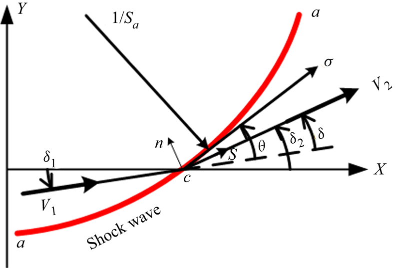
 $a$ in the flow plane is presented in the Cartesian coordinate system, as shown in figure 2. The
 $x$-axis is parallel to the symmetry axis of the planar/axis symmetry shock. The
 $y$-axis is perpendicular to the
 $x$-axis. The velocity angles
 $\delta _1$ and
 $\delta _2$ in figure 2 are the acute angles between the velocity vectors and the
 $x$-axis, and the flow deflection angle
 $\delta$ is calculated as
 $\delta = {\delta _2} - {\delta _1}$. Similarly, the shock angle
 $\theta$ is defined as the angle by which the line
 $a$–
 $a$ is inclined to the incoming velocity vector
 $\boldsymbol {V}_1$. According to the geometric relations, the inclination angle of the shock
 $a$–
 $a$ to the
 $x$-axis,
 $\theta _1$, is equal to the shock angle plus the pre-shock velocity angles (
 $\theta _1=\theta +\delta _1$). The length
 $\sigma$ is the distance measured along the trace
 $a$–
 $a$. The lengths
 $s$ and
 $n$ are the distances measured along and perpendicular to the streamline, respectively. Based on these variables, the variable
 $S_{a}$, which represents the curvature of the shock wave in the flow plane, is given by
 ${S_{a}} = - 1/{R_{a}} = \partial {\theta _1}/\partial \sigma$, where
 $R$ is the radius of curvature. Similarly, the curvature of the shock wave in the flow-normal plane is
 ${S_{b}} = - 1/{R_{b}} = - \cos {\theta _1}/y$, where
 $y$ is the distance from the shock wave to the
 $x$-axis.
Geometry of curved shock from the paper by Mölder (Reference Mölder2016).

Variables in the flow plane from the paper by Shi et al. (Reference Shi, Han, Deiterding, Zhu and You2020).

To clarify the derivation of the curved shock equations, Mölder introduced the following normalized variables:
 \begin{equation}
\left.\begin{array}{rl@{}} \text{normalized pressure
gradient:} & P = (\partial p/\partial s)/\rho
{V^2};\\ \text{streamline curvature:} &
D = \partial \delta /\partial s;\\
\text{normalized vorticity:}& \varGamma = \omega
/V; \end{array}\right\}
\end{equation}
where  $p$,
 $\rho$,
 $V$ and
 $\omega$ represent the local static pressure, density, velocity and vorticity, respectively.
In terms of these variables, the Euler equations for steady flow become
 $$\begin{align} \text{mass:}& \quad\frac{{\partial \delta }}{{\partial n}} ={-} ( {{M^2} - 1} )P - j\frac{{\sin \delta }}{y}; \end{align}$$
 $$\begin{align}s\text{-momentum:} &\quad
\frac{1}{V}\frac{{\partial V}}{{\partial s}} ={-}
\frac{1}{{\rho {V^2}}}\frac{{\partial p}}{{\partial s}}
={-} P; \end{align}$$
 $$\begin{align}n\text{-momentum:}& \quad\frac{1}{{\rho {V^2}}}\frac{{\partial p}}{{\partial n}} ={-} \frac{{\partial \delta }}{{\partial s}} ={-} D; \end{align}$$
 $$\begin{align}\text{energy:} &
\quad\left.\begin{array}{l@{}} \displaystyle\dfrac{1}{\rho }\dfrac{{\partial \rho }}{{\partial n}} ={-}
{M^2}[ {D + ( {\gamma - 1} )\varGamma }], \\
\displaystyle \dfrac{1}{\rho }\dfrac{{\partial \rho }}{{\partial s}} =
{M^2}P;\end{array}\right\}
\end{align}$$
 $$\begin{align}\text{vorticity:}& \quad\frac{1}{V}\frac{{\partial V}}{{\partial n}} = D - \varGamma; \end{align}$$
where  $M$ and
 $\gamma$ denote the local Mach number and ratio of specific heat, respectively.
In these equations, all variables have a subscript of either 1 or 2 depending on whether they represent the pre- or post-shock condition. As the variable  $y$ has the same value on opposite sides of the same shock, no subscript is necessary for this variable. The use of
 $j$ to indicate planar (0) or axially (1) symmetric flow is neglected from this point on. Applying these relations to the Rankine–Hugoniot (R–H) equations,
 $$\begin{gather} \frac{{{p_2}}}{{{p_1}}} = \frac{{2\gamma }}{{\gamma + 1}}M_1^2 \sin ^2 \theta - \frac{{\gamma - 1}}{{\gamma + 1}}, \end{gather}$$
 $$\begin{gather}{p_1} + {\rho_1}V_1^2 \sin ^2 \theta = {p_2} + {\rho_2}V_2^2 \sin ^2 ( {\theta - \delta } ), \end{gather}$$
generates (after considerable algebraic manipulation) the curved shock equations
 $$\begin{gather} {A_1}{P_1} + {B_1}{D_1} + {E_1}{{ \varGamma }_1} = {A_2}{P_2} + {B_2}{D_2} + C{S_{a}} + G{S_{b}}, \end{gather}$$
 $$\begin{gather}A_1^\prime {P_1} + B_1^\prime {D_1} + E_1^\prime {{ \varGamma }_1} = A_2^\prime {P_2} + B_2^\prime {D_2} + C'{S_{a}} + G'{S_{b}}. \end{gather}$$
Here, the coefficients  $A$,
 $B$,
 $C$,
 $E$ and
 $G$ are functions of the shock angle and the incoming flow condition. Expressions of these coefficients and derivation details of (2.2)–(2.10) have been given by Mölder (Reference Mölder2016). Furthermore, taking the derivative with respect to
 $\sigma$ of both sides of each of the first-order curved shock equations gives the second-order curved shock equations:
 $$\begin{gather} A_1^{\prime \prime } P_1^\prime + B_1^{\prime \prime } D_1^\prime + E_1^{\prime \prime }{{ \varGamma }_1}^\prime = A_2^{\prime \prime } P_2^\prime + B_2^{\prime \prime } D_2^\prime + C^{\prime \prime } S_{a}^\prime + G^{\prime \prime } S_{b}^\prime + \mathrm{const.}^{\prime \prime }, \end{gather}$$
 $$\begin{gather}A_1^{\prime \prime \prime } P_1^\prime + B_1^{\prime \prime \prime } D_1^\prime + E_1^{\prime \prime \prime }{{ \varGamma }_1}^\prime = A_2^{\prime \prime \prime } P_2^\prime + B_2^{\prime \prime \prime } D_2^\prime + C^{\prime \prime \prime } S_{a}^\prime + G^{\prime \prime \prime } S_{b}^\prime + \mathrm{const.}^{\prime \prime \prime }. \end{gather}$$
Details of the derivation of the second-order curved shock equations and their coefficients have been given by Shi et al. (Reference Shi, Han, Deiterding, Zhu and You2020).
2.2. Derivation of MOCC equations
Curved shock theory gives the shock curvature and flow divergence/convergence in terms of the first- and second-order gradients of pressure, vorticity and streamline curvature. Once the incoming flow condition has been determined, the post-shock parameters can be solved using the curved shock equations. However, the curved shock equations are only tenable near the shock. To calculate the supersonic flowfields, the MOCC equations are derived in the streamline–characteristic ( $s$–
 $l$,
 $s$ for streamline,
 $l$ for characteristic) coordinates.
The Euler equations (2.2)–(2.6) are applicable for supersonic flowfields. Therefore, combining similar terms in (2.3) produces the momentum equation along the streamline,
 \begin{equation} \rho V{\frac{\partial V}{\partial s}}+{\frac{\partial p}{\partial s}} = 0.\end{equation}
Similarly, the energy equation along the streamline, generated from (2.5), is
 \begin{equation} {\frac{\partial p}{\partial s}}-{\frac{\gamma p}{\rho}} {\frac{\partial \rho}{\partial s}} = 0. \end{equation}
The momentum equation along characteristic lines and the mass equation are derived by taking the derivative with respect to  $l$ of the pressure and flow deflection angle. To replace the
 $l$-derivatives in the differentiated conservation equations by
 $s$- and
 $n$-derivatives, the derivative of any quantity with respect to distance along left-running and right-running characteristics can be written in terms of the two derivatives along and normal to the streamline, as follows:
 \begin{equation} {\left( {\frac{{\partial \bullet }}{{\partial l }}} \right)_\pm} = {\left( {\frac{{\partial \bullet }}{{\partial s}}} \right)}\cos \mu \pm {\left( {\frac{{\partial \bullet }}{{\partial n}}} \right)}\sin \mu,\end{equation}
where  $\mu$ is the included angle of streamlines and characteristics. The subscript
 $\pm$ denotes a left-running
 $(+)$ or right-running
 $(-)$ characteristic line. The symbols
 $\pm$ and
 $\mp$ take the upper or lower part depending on whether the equation is used along the left-running or right-running characteristic line. This gives
 \begin{equation} {\left( {\frac{{\partial p }}{{\partial l }}} \right)_\pm} = {\left( {\frac{{\partial p }}{{\partial s}}} \right)}\cos \mu \pm {\left( {\frac{{\partial p }}{{\partial n}}} \right)}\sin \mu.\end{equation}
Substituting the definitions into (2.16) gives the momentum equation along the characteristic line,
 \begin{align} {\left( {\frac{{\partial p }}{{\partial l }}} \right)_\pm} &= \rho V^2 P \cos \mu \mp \rho V^2 D \sin \mu \nonumber\\ &= \rho V^2 ( P \cos \mu \mp D \sin \mu ). \end{align}
As for the mass equation in the  $s$–
 $l$ coordinates, taking the derivative of the flow deflection angle with respect to
 $l$ produces
 \begin{equation} {\left( {\frac{{\partial \delta }}{{\partial l }}} \right)_\pm} = {\left( {\frac{{\partial \delta }}{{\partial s}}} \right)}\cos {\mu } \pm {\left( {\frac{{\partial \delta }}{{\partial n}}} \right)}\sin {\mu }.\end{equation}
Similar to the treatment of the momentum equation along the characteristic line, the mass equation can be reformulated as
 \begin{align} {\left( {\frac{{\partial \delta }}{{\partial l }}} \right)_\pm} &= D \cos {\mu } \mp \left( \frac{P}{\tan^2\mu}+j\frac{\sin\delta}{y}\right)\sin {\mu } \nonumber\\ &= \frac{D\sin {\mu } \mp P\cos {\mu }}{\tan\mu} \mp j\frac{\sin\delta \sin {\mu }}{y}. \end{align}
Equations (2.13), (2.14), (2.17) and (2.19), together with the gradients of pressure and flow deflection angle,  $P = (\partial p/\partial s)/\rho {V^2}$ and
 $D = \partial \delta /\partial s$, form the system of partial differential equations of MOCC.
Based on the total differential relation, the variation of parameters between two points can be resolved in terms of differences along and normal to the streamline. Consider the pressure as an example. The pressure change between two points behind the shock can be represented as follows:
 \begin{equation} \mathrm{d}p= {\left( {\frac{{\partial p }}{{\partial s}}} \right)}\, \mathrm{d}s + {\left( {\frac{{\partial p }}{{\partial n}}} \right)}\,\mathrm{d}n. \end{equation}
When these two points lie on the same streamline,  $\mathrm {d}n$ is equal to zero. Equation (2.20) can then be simplified to
 $\mathrm {d}p / \mathrm {d}s={\partial p } / {\partial s }$. This relation is suitable for the other variables. Therefore, along a streamline or a characteristic line, the partial derivative of a parameter, with respect to
 $s$ or
 $l$, is equivalent to the total derivative of that variable. With this relation, the partial differential equations of MOCC can be transformed into total differential equations for the same streamline and characteristic:
 \begin{equation} \left.\begin{array}{c@{}}
\displaystyle {\dfrac{\mathrm{d} p}{\mathrm{d} l_\pm}} -
\rho V^2 ( P\cos \mu \mp D \sin \mu) = 0,\\ \displaystyle
{\dfrac{\mathrm{d} \delta}{\mathrm{d} l_\pm}}-\dfrac{D \sin
\mu \mp P\cos \mu}{\tan \mu} \pm j\dfrac{\sin \delta \sin
\mu}{y} =0,\\ \displaystyle {\dfrac{\mathrm{d}
p}{\mathrm{d} s}}-\rho V^2 P =0,\\ \displaystyle
{\dfrac{\mathrm{d} \delta}{\mathrm{d} s}}-D =0,\\
\displaystyle \rho V{\dfrac{\mathrm{d} V}{\mathrm{d}
s}}+{\dfrac{\mathrm{d} p}{\mathrm{d} s}} = 0,\\
\displaystyle {\dfrac{\mathrm{d} p}{\mathrm{d}
s}}-{\dfrac{\gamma p}{\rho}} {\dfrac{\mathrm{d}
\rho}{\mathrm{d} s}} = 0. \end{array}\right\}
\end{equation}
From the total differential equations (2.21), there are six unknowns,  $p$,
 $\delta$,
 $\rho$,
 $V$,
 $P$ and
 $D$, for six equations describing a unit process containing a streamline and a characteristic. Therefore, MOCC extends the application area of curved shock theory from the region near the shock to the post-shock flowfield. Furthermore, unlike MOC, which needs two characteristics and one streamline for iterations, only one characteristic and one streamline are required to solve the MOCC equations. Specifically, the supersonic external and internal flowfields depend on the left-running and right-running characteristics, respectively. Thus, the equations for the left-running characteristic and streamline are solved in
 $s - l_+$ coordinates for the external flow, whereas the equations of the right-running characteristic and streamline are evaluated in
 $s - l_-$ coordinates for the internal flow. As MOCC only uses two lines (one characteristic and one streamline) in the unit process, no iterations are required for the determination of the third line, which is an essential procedure in MOC. The unsolved point can be directly calculated from the information of two nodes. This advantage makes MOCC a simple and time-saving method for flowfield calculations. Additionally, MOCC relates the gradients of pressure and flow deflection angle to the flow parameters. As a result, the pressure and flow deflection angle, as well as their gradients, can be acquired over the whole flowfield. Gradients, such as
 $P$ and
 $D$, are important variables for flow analysis because they describe changes to the flow variables. With this information, only a small number of mesh nodes are required to solve the whole flowfield. These gradients can also be used to investigate physical phenomena such as shock reflection. For instance, a regular shock reflection occurs in planar internal flow without a centre-body, whereas in axisymmetric internal flow without a centre-body, only an irregular shock reflection can appear. It is the gradients that produce these different characteristics in planar and axisymmetric flows. Therefore, the gradients obtained from MOCC offer a new perspective for the analysis of shock structures. Additionally, based on the von Neumann condition, the quantity
 $M^2P/D$ must remain the same across the slip layer. Thus, the variables
 $P$ and
 $D$ in the whole flowfield offer a novel perspective for analysing the physical characteristics of the slip layer.
2.3. Algorithms
Considering their practical importance, inverse problems, such as calculations with given shocks, have aroused widespread interest. Nowadays, CFD is a common means of acquiring the supersonic flowfield, but it can only be applied to direct designs that determine the flowfield with a given wall. MOC is a numerical method of solving the inviscid flowfield based on the characteristic equations and compatibility relations. It is tedious because the compatibility equations are solved along three characteristics (two characteristics and one streamline). In the MOC numerical scheme, the position of the unsolved point is determined by two given nodes. As two nodes can only determine two characteristics, another characteristic or streamline through this unsolved point is needed to solve the equations. Furthermore, the third characteristic needs to be solved repeatedly during the iteration process. Thus, extra iterations are needed to calculate the third characteristic, which makes MOC complex and only weakly robust. The use of MOCC to solve the planar and axisymmetric flowfields reduces the computational resources required, as MOCC only requires one characteristic and one streamline to solve the equations. Owing to this benefit, the iteration process is simple and saves a considerable amount of resources. Three unit algorithms are introduced.
2.3.1. Interior process
In MOCC, the only difference between the external and internal interior processes is the selection of the characteristics. Therefore, the interior process is first presented in the case of external flow. For external flow, the second-order central difference form of the total differential equations are presented as follows:
 \begin{equation} \left.\begin{array}{c@{}}
\displaystyle {\dfrac{{\Delta} p}{{\Delta}
l}} - \bar{\rho} \bar{V}^2 ( \bar{P}\cos \bar{\mu} -\bar{D}
\sin \bar{\mu}) = 0,\\ \displaystyle
{\dfrac{{\Delta} \delta}{{\Delta}
l}}+\dfrac{\bar{P}\cos \bar{\mu} -\bar{D} \sin
\bar{\mu}}{\tan \bar{\mu}}+j\dfrac{\sin \bar{\delta} \sin
\bar{\mu}}{\bar{y}} =0,\\ \displaystyle
{\dfrac{{\Delta} p}{{\Delta} s}}-\bar{\rho}
\bar{V}^2 \bar{P} =0,\\ \displaystyle
{\dfrac{{\Delta} \delta}{{\Delta}
s}}-\bar{D} =0,\\ \displaystyle \bar{\rho}
\bar{V}{\dfrac{{\Delta} V}{{\Delta}
s}}+{\dfrac{{\Delta} p}{{\Delta} s}} = 0,\\
\displaystyle {\dfrac{{\Delta} p}{{\Delta}
s}}-{\dfrac{\gamma \bar{p}}{\bar{\rho}}}
{\dfrac{{\Delta} \rho}{{\Delta} s}} = 0,
\end{array}\right\}
\end{equation}
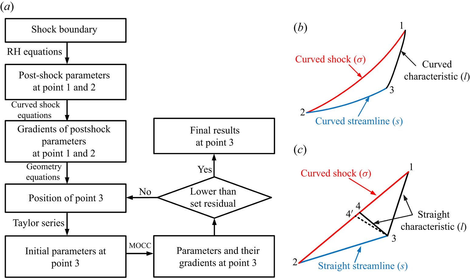
where the superscript  $\bar {\quad }$ represents the average value of two discrete points. Figure 3(a) illustrates the MOCC scheme for the interior process in planar and axisymmetric flows. The red, blue and black curves denote the shock, streamline and characteristic, respectively. Figure 3(b) shows a flowchart of the MOCC interior process in planar and axially symmetric flows. As the incoming flow condition and the geometry of the shock wave are known, the post-shock aerodynamic parameters, such as pressure and flow deflection angle at points 1 and 2, can be solved based on the R–H relations. These parameters and the shock wave curvatures are then used to calculate the post-shock gradients of pressure and flow deflection angle at points 1 and 2 using curved shock equations. After the physical information at points 1 and 2 has been determined, the position of point 3 is solved using the following geometric equations:
 \begin{equation} \left.\begin{array}{c@{}} \displaystyle x_{p3}=\dfrac{y_{p2}-\tan (\delta_{p2}) x_{p2}-y_{p1}+\tan (\delta_{p1}+\mu_{p1})x_{p1}}{\tan (\delta_{p1}+\mu_{p1})-\tan (\delta_{p2})},\\ y_{p3}=\tan (\delta_{p2})x_{p3}+y_{p2}-\tan (\delta_{p2}) x_{p2}, \end{array}\right\} \end{equation}
where the subscripts  $p1$,
 $p2$ and
 $p3$ denote points 1, 2 and 3. Once the position of point 3 has been determined, the initial values of the aerodynamic parameters can be calculated at point 2 as
 \begin{equation} \left.\begin{array}{c@{}} \delta_{p3}=\delta_{p2}+(s_{p3}-s_{p2})D_{p2},\\ p_{p3}=p_{p2}+(s_{p3}-s_{p2})\rho_{p2} V_{p2}^2 P_{p2}. \end{array}\right\} \end{equation}
Next, the second-order central differential equations (2.22) are solved with the variables at points 1, 2 and 3 to obtain new aerodynamic parameters at point 3. If the differences between the old and new aerodynamic parameters are greater than the set residuals, the position and aerodynamic parameters at point 3 will be resolved using the average values of points 2 and 3 through the iterative approach. Through this iterative process, the aerodynamic parameters and their gradients will converge to the actual values.
Interior process and flowchart. (a) Flowchart of MOCC, (b) unit process of MOCC and (c) unit process of MOC.

Using the gradients makes the MOCC interior process simpler and more accurate than the MOC interior process shown in figure 3(c). In the MOC interior process, only the flow parameters at points 1 and 2 are known, so the streamline and characteristics are straight lines. The initial values at point 3 are always the same as those of point 2. As the compatibility equations of MOC must be solved along two characteristics and one streamline, another characteristic ‘34’ has to be calculated before the iteration of point 3. The initial flow parameters at point 4 are acquired from the linear interpolation of points 1 and 2. With these new values, iterations are necessary to change the location of point 4 to 4’. The compatibility equations are then solved with the flow parameters at points 1, 2, 3 and 4’ to obtain new values at point 3. As the values at point 3 change, the position of point 4 has to be recalculated through the iterative process. The calculations of points 3 and 4 are repeated in the MOC interior process. Thus, from the calculation steps, MOCC provides a better initial value of point 3 than MOC, and so fewer iterations are required to acquire convergent results. Furthermore, MOCC does not use the characteristic 34 to solve the second-order central differential equations (2.22). Removing the iterations and deviations for the calculation of point 4 reduces the computational expense and increases the precision of the MOCC interior process. Thus, MOCC not only reduces the computation time but also enhances the accuracy of the calculations by using the gradients.
2.3.2. Wall/parameter distribution process
As the wall boundary can be regarded as the flow angle distribution, the unit process of the wall boundary is the same as the parameter distribution process for MOCC. In this section, the parameter distribution process is illustrated for generality. All aerodynamic parameters can be identified because, along the streamline, they are connected by isentropic rules. The transformation equations are listed as follows:
 \begin{equation} \left.\begin{array}{c@{}} \displaystyle p(1+\dfrac{\gamma-1}{2}M^2)^{\gamma/(\gamma-1)}=\textrm{const.},\\ \dfrac{p}{\rho^\gamma}=\textrm{const.} \end{array}\right\} \end{equation}
For internal flow, the second-order central difference form of the total differential equations can be written as follows:
 \begin{equation} \left.\begin{array}{c@{}} \displaystyle {\dfrac{{\Delta} p}{{\Delta} l}} - \bar{\rho} \bar{V}^2 ( \bar{P}\cos \bar{\mu} +\bar{D} \sin \bar{\mu}) = 0,\\ \displaystyle {\dfrac{{\Delta} \delta}{{\Delta} l}}-\dfrac{\bar{P}\cos \bar{\mu} -\bar{D} \sin \bar{\mu}}{\tan \bar{\mu}}-j\dfrac{\sin \bar{\delta} \sin \bar{\mu}}{\bar{y}} =0,\\ \displaystyle {\dfrac{{\Delta} p}{{\Delta} s}}-\bar{\rho} \bar{V}^2 \bar{P} =0,\\ \displaystyle {\dfrac{{\Delta} \delta}{{\Delta} s}}-\bar{D} =0,\\ \displaystyle \bar{\rho} \bar{V}{\dfrac{{\Delta} V}{{\Delta} s}}+{\dfrac{{\Delta} p}{{\Delta} s}} = 0,\\ \displaystyle {\dfrac{{\Delta} p}{{\Delta} s}}-{\dfrac{\gamma \bar{p}}{\bar{\rho}}} {\dfrac{{\Delta} \rho}{{\Delta} s}} = 0, \end{array}\right\} \end{equation}
where the superscript  $\bar {\quad }$ represents the average value of two discrete points.
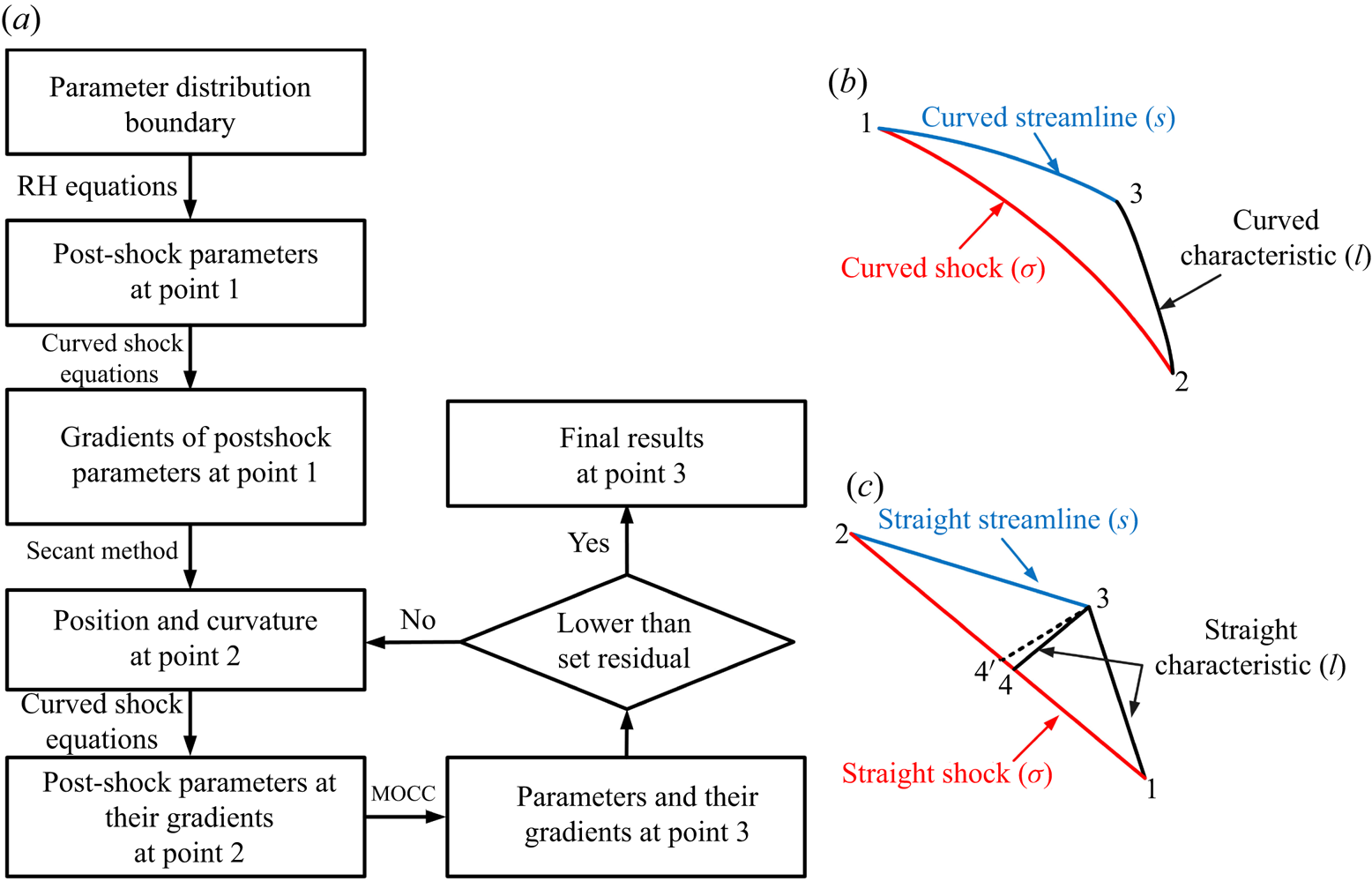
Figure 4(a) shows the MOCC scheme for the parameter distribution process in planar and axially symmetric flows. As above, the red, blue and black curves denote the incident shock, streamline (wall) and characteristic, respectively. Figure 4(b) shows a flowchart of the MOCC parameter distribution process in planar and axially symmetric flows. As the incoming flow condition and the parameter distribution are known, the post-shock aerodynamic parameters, such as the pressure and flow deflection angle at point 1, can be solved based on the R–H relations. Furthermore, the gradient of pressure  $P$ (or the streamline curvature
 $D$) and the transverse curvature
 $S_b$ can be acquired from the parameter distribution. These parameters are used to calculate the post-shock gradients and streamwise shock curvature at point 1 using the curved shock equations. Once the physical parameters at point 1 have been obtained, the position and curvatures at point 2 can be acquired using the secant method. From the curvatures and incoming condition, the post-shock parameters and their gradients can then be solved with the R–H relations and curved shock equations at point 2. The position of point 3 is acquired using the following geometric equations:
 \begin{equation} \left.\begin{array}{c@{}} \displaystyle x_{p3}=\dfrac{y_{p1}-\tan (\delta_{p1}) x_{p1}-y_{p2}+\tan (\delta_{p2}-\mu_{p2})x_{p2}}{\tan (\delta_{p2}-\mu_{p2})-\tan (\delta_{p1})},\\ y_{p3}=\tan (\delta_{p1})x_{p3}+y_{p1}-\tan (\delta_{p1}) x_{p1}, \end{array}\right\} \end{equation}
where the subscripts  $p1$,
 $p2$ and
 $p3$ denote points 1, 2 and 3. After the position of point 3 has been determined, the initial values of the aerodynamic parameters can be obtained by using the Taylor series equations (2.24) at point 1. The next step is to solve the second-order central differential equations (2.26) with the variables at points 1, 2 and 3 to obtain new aerodynamic parameters at point 3. If the differences between the solved and actual aerodynamic parameters are greater than the set residuals, the position and curvatures at point 2 will be resolved with the secant method until the deviations are less than the set residuals. After this iterative process, the aerodynamic parameters and their gradients will converge to the actual values.
Wall/parameter distribution process and flowchart. (a) Flowchart of MOCC, (b) unit process of MOCC and (c) unit process of MOC.

Similar to the interior process, the MOC wall/parameter distribution process still needs to calculate the characteristic line 34 before solving the compatibility equations. Without gradients, the characteristics and streamline are straight lines in the MOC wall/parameter distribution process. With the linear interpolation method, moving the location of point 4 to 4’ is repeated in every iteration of the compatibility equations. The deviation in the calculation of point 4 is accumulated in the results at point 3, which decreases the accuracy of the MOC wall/parameter distribution process. The MOCC wall/parameter distribution process, in which the gradients indicate the change in the flow parameters, acquires a better initial value of point 3 than MOC. Additionally, MOCC does not require characteristic 34 to solve the second-order central differential equations (2.26). As a result, only a small number of iterations are needed for MOCC to acquire the flow parameters and their gradients at point 3. Again, MOCC not only reduces the computation time, but also enhances the accuracy of the calculation by using the gradients.
2.3.3. Shock process
There is a third process involving the shock for the flowfield calculation. The second-order central difference form of the total differential equations is
 \begin{equation} \left.\begin{array}{c@{}} \displaystyle {\dfrac{{\Delta} p}{{\Delta} \sigma}} - \bar{\rho} \bar{V}^2 ( \bar{P}\cos \bar{\theta} -\bar{D} \sin \bar{\theta} ) = 0,\\ \displaystyle {\dfrac{{\Delta} \delta}{{\Delta} \sigma}}+\dfrac{\bar{P}\sin \bar{\theta} }{\tan ^2 \bar{\mu}}-\bar{D}\cos\bar{\theta}+j\dfrac{\sin \bar{\delta} \sin \bar{\theta}}{\bar{y}} =0,\\ \displaystyle {\dfrac{{\Delta} p}{{\Delta} s}}-\bar{\rho} \bar{V}^2 \bar{P} =0,\\ \displaystyle {\dfrac{{\Delta} \delta}{{\Delta} s}}-\bar{D} =0,\\ \displaystyle \bar{\rho} \bar{V}{\dfrac{{\Delta} V}{{\Delta} s}}+{\dfrac{{\Delta} p}{{\Delta} s}} = 0,\\ \displaystyle {\dfrac{{\Delta} p}{{\Delta} s}}-{\dfrac{\gamma \bar{p}}{\bar{\rho}}} {\dfrac{{\Delta} \rho}{{\Delta} s}} = 0, \end{array}\right\} \end{equation}
where the superscript  $\bar {\quad }$ represents the average value of two discrete points.
Figure 5(a) illustrates the MOCC scheme of the shock process to determine the flow pattern near the shock. The shock, streamline and characteristic are represented by red, blue and black curves, respectively. Although the parameters and their gradients at points 1 and 2 are known, another condition is needed for the shock process. This condition should have some relation with the shock, such as the geometry of the reflected shock, post-shock parameters and so on. For most conditions, a horizontal flow is desirable. Therefore, the flow deflection angle behind the shock is chosen as a known condition for this unit process. Note that other information about the shock can also be used as a known condition, but some details of the unit process change according to different conditions. However, the overall scheme remains similar. Figure 5(b) shows a flowchart of the MOCC shock process. As the physical conditions of points 1 and 2 are known, the first step of this unit process is to obtain the position and curvature of point 3. The secant method is used to solve the shock angle of point 3. With the shock angle, the position of point 3 can be calculated using the following geometric equations:
 \begin{equation} \left.\begin{array}{c@{}} \displaystyle x_{p3}=\dfrac{y_{p2}-\tan (\delta_{p2}) x_{p2}-y_{p1}+\tan (\theta_{p1})x_{p1}}{\tan (\theta_{p1})-\tan (\delta_{p2})},\\ y_{p3}=\tan(\delta_{p2})x_{p3}+y_{p2}-\tan (\delta_{p2}) x_{p2}, \end{array}\right\} \end{equation}
where the subscripts  $p1$,
 $p2$ and
 $p3$ denote points 1, 2 and 3, respectively. The initial values at point 3 are acquired with the R–H relations based on the known information of the shock. The following step involves solving the second-order central differential equations (2.28) with the variables at points 1, 2 and 3 to obtain new aerodynamic parameters and their gradients at point 3. Once the differences between the solved and actual aerodynamic parameters are less than the set residuals, the iterative process terminates, and the convergent aerodynamic parameters and their gradients at point 3 are obtained.
Shock process and flowchart. (a) MOCC flowchart, (b) unit process of MOCC and (c) unit process of MOC.

Different from the MOC shock process shown in figure 5(c), the use of gradients in the MOCC shock process means that the characteristic, streamline and shock are curved lines. This provides a better initial value at point 3 and reduces the number of iterations required for the calculation of flow parameters. As the MOCC shock process only uses one characteristic and one streamline to solve the second-order central differential equations (2.28), it is not necessary to solve the position of another characteristic, 34. For MOC, it is the determination of the characteristic 34 that introduces additional complexity and deviations to the flow parameters at point 3. Once again, the use of gradients in the MOCC shock process results in greater efficiency and accuracy.
3. Verification of algorithms
The curved shock equations give explicit answers in the neighbourhood close to the shock waves. With the boundary condition from the curved shock equations, MOCC can be used to solve the planar and axially symmetric flowfields with a high degree of accuracy. Planar/axisymmetric supersonic flowfields are presented to show the benefits of MOCC. The generality of MOCC can be demonstrated by applying the scheme to non-uniform flows. MOC and CFD are used as references.
3.1. Planar flows
3.1.1. Uniform external flow with known shock boundary condition
Consider a unit process in which only the information at the endpoints of the shock wave is known, which is common in the field of adaptive mesh refinement. A unit mesh is refined, and the flowfield is solved by MOC and MOCC in this unit process. For quantitative analysis, the planar curved shock in this unit mesh is given explicitly as  $y =\frac 12 (\mathrm {e}^x-1)$. MOC is used to solve the flowfield behind the explicit shock. For clarity, the flowfield solved by MOC, under the condition that the whole shock wave is known explicitly, is named the reference flowfield. For a unit process in which only the information at the endpoints of the shock wave is given, the shock wave has to be fitted and refined. The post-shock parameters and their gradients are calculated at the beginning and end of the shock curve at an incoming Mach number of 5. For MOC, which only acquires the shock wave angles together with the positions of the given two nodes before the shock refinement, the shock wave is fitted with a cubic equation
 $y = 0.1415{x^3} + 0.217{x^2} + 0.5006x$. MOCC gives the shock angles and the curvatures at these two nodes before the shock refinement. The shock wave angle is connected to the slope of the shock wave, and the second derivative
 $y^{\prime \prime }$ can be obtained from the curvatures. For the unit flowfield solved using MOCC, the shock wave is fitted by a quintic equation
 $y = 0.007{x^5} + 0.0176{x^4} + 0.0845{x^3} + 0.2500{x^2} + 0.5x$. The fitted shock wave is then refined with 40 points and used to solve the unit flowfield.
Figure 6 shows the planar flowfields obtained by the two different methods with the given parameters at the endpoints of the shock wave. The reference flowfield is represented by the coloured areas and black solid lines. The grey and red dashed curves in figure 6 represent the flowfields obtained using MOC and MOCC, respectively. For planar flow, the cross-sectional geometry of the curved shock is a line, which means that there is no curvature in the flow-normal plane of the shock wave. From the figure, it is clear that the flowfield obtained using MOCC has a similar character to the reference flowfield. The isoparametric curves of MOCC have a greater coincidence with those of the reference flowfield than those of MOC, which demonstrates the merit of MOCC in increasing the accuracy with fewer nodes. Furthermore, MOCC provides more information than MOC by solving the gradients. As the gradients describe the flow tendency, they can be used to increase the accuracy of the results and analyse the flow pattern. This is a great advantage of MOCC over MOC.
Flowfields calculated using MOC and MOCC in uniform planar flow ( $y =\frac 12 (\mathrm {e}^x-1), x\in [0,1]$).

For quantitative analysis, the results of a regression analysis are presented in table 1. The residual sum of squares (RSS) indicates the degree of fit of the sample values to the contrast results. This is the sum of the squares of the deviations between the sample values and the contrast results. As MOC is known to be highly accurate, the reference flowfield data given by MOC with  $118 \times 118$ nodes are considered as the contrast results. Furthermore, the goodness of fit (
 $R^{2}$) is a statistical model describing the similarity between sample values and reference results, and ranges from 0 to 1. A large value of
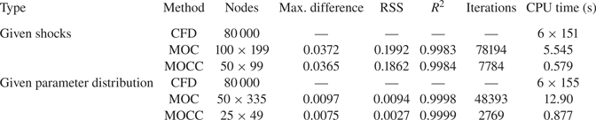
 $R^2$ indicates a tight fit. From table 1, it is clear that for the planar flow, the maximum difference decreases from 0.0206 with MOC to 0.0002 with MOCC. The RSS for MOC with
 $118 \times 118$ nodes is 0.0520, which is approximately four orders of magnitude greater than that for MOCC with
 $40 \times 40$ nodes. This means that MOCC offers improved accuracy. The
 $R^2$ value increases from 0.9995 (MOC with
 $118 \times 118$ nodes) to 1.0000 (MOCC with
 $40 \times 40$ nodes), which confirms that the planar flowfield solved by MOCC is closer to the reference flowfield. Statistically, the planar flowfield obtained from MOCC can be considered to be the same as that of the reference. Therefore, in comparison with MOC, the proposed MOCC achieves higher precision with fewer mesh nodes.
Regression analysis of MOCC in planar, uniform external flow.

As well as its high precision, MOCC also offers high computational efficiency. The number of iterations and the calculation time of MOC and MOCC in planar flow are compared in table 1. For planar flow, MOC takes 0.906 s to solve a flowfield with  $118\times 118$ nodes in 41 418 iterations. By contrast, MOCC with
 $40 \times 40$ nodes only requires 0.107 s to acquire the same flowfield in just 780 iterations. Thus, the use of gradients significantly reduces the computation time and number of iterations for planar flow. There are two reasons for this high computational efficiency. One is that a better initial value can be acquired using gradients, because the gradients reflect the flow trend. When an initial value is closer to the solution, fewer iterations are required to solve the equations. The second reason is that MOCC needs only one characteristic line and one streamline to solve the equations in every unit process. This calculation scheme is greatly simplified compared with MOC, which requires one streamline and two characteristics to determine the solutions in every unit process. As two known points can only determine two of those three lines (one streamline and two characteristics), iterations are required to obtain the third line. This complexity incurs a great number of iterations in MOC. However, the price of simplifying the scheme is to increase the number of equations from four to six. Therefore, each iteration of MOCC takes longer. In MOCC, the major part of the CPU time is taken up by solving the curved shock equations. From the above comparison, MOCC can reduce the computation time by approximately 90 % for the same accuracy. With the same number of mesh nodes, MOCC can acquire a more accurate planar flowfield in a shorter time than MOC. Although the absolute decrease in computation time is less than 1 s in this example, the relative variation is considerable, especially when one considers that optimization problems can take several days to solve tens of thousands of flowfields. MOCC can reduce the required resources by approximately 90 % in such situations.
3.1.2. Uniform internal flow with known parameter distribution as boundary condition
Similarly, MOCC can be applied to a uniform internal flow with a given parameter distribution on the wall. The solved flowfields given by MOC and MOCC are compared with the numerical results from CFD. As CFD is mainly used in the direct design, the wall connected to the given pressure distribution is first calculated using MOC and MOCC, and then the flow around the wall is simulated with CFD. As viscosity is neglected in this study, the inviscid model is chosen. The inviscid flux is solved using Roe's flux differencing scheme. Second-order upwind discretization with a fully implicit scheme is used to calculate the governing equations. A limiter is added to the spatial discretization for the suppression of the numerical oscillation. The structured grid is shown in figure 7, where the actual mesh density has been reduced for clarity. The real grid for the model contains approximately 80 000 cells after the grid-independence verification. The grid resolution is sufficient to acquire grid-converged results. Inflow boundary conditions are set to the far-field pressure with the values of the freestream parameters, and outflow boundary conditions are set to the pressure outlet. In this research, a calorically perfect gas model is assumed. A slip condition is applied to the wall boundary. The convergence principle is that each residual should be reduced by at least three orders of magnitude, and the mass flow rate should be conserved at the outlet. The flow characteristics of the planar flowfields with the given pressure distribution along the wall at an incoming Mach number of 6 are shown in figure 8. The planar pressure distribution along the wall is a curve given by the equation  $p/p_0=x^2+3x+4$. The black solid lines denote the isoparametric curves and shocks of the CFD results, whereas the isoparametric curves of MOC and MOCC are represented by grey and red dashed curves, respectively. The given wall is illustrated with a blue dashed curve. The excellent agreement between the black solid curves and the red dashed curves indicates that MOCC's flowfield is extremely similar to the CFD results. Thus, MOCC offers high accuracy in applications where the parameter distribution is used for the calculations.
Grid structure and boundary conditions.

Planar internal flowfields calculated with a given parameter distribution in uniform flow ( $p/p_0=x^2+3x+4$).

The results of a regression analysis are presented in table 2. MOC and MOCC calculated the planar flowfield using  $50\times 324$ nodes and
 $25\times 49$ nodes, respectively. The CFD results corresponding to these nodes are extracted as the contrast data. From the table, the maximum differences in Mach number given by the MOC and MOCC planar flowfields are 0.0111 and 0.0102, respectively. The RSS and
 $R^2$ values are 0.0053 and 0.9999 for MOC and 0.0032 and 0.9999 for MOCC, respectively. These variables indicate that, on average, the Mach number difference of every node in the planar flowfield given by MOCC is less than in that given by MOC. The similarity between the planar flowfields calculated by MOCC and CFD is 99.99 %, the same as for MOC. Statistically, MOCC obtains the same solution as MOC using fewer mesh nodes. Furthermore, MOCC only takes 0.584 s to acquire the results. By contrast, MOC requires 12.30 s, which is more than 20 times as long. Thus, compared with MOC, MOCC is both more accurate and more efficient for planar flowfield calculations with a given parameter distribution. As for CFD, the wall time (145 s) multiplied by the number of parallel cores (6) gives the CPU time, which is three orders of magnitude higher than that of MOCC. CFD has the advantage of high generality. Complex flowfields containing supersonic and subsonic flows can be solved by CFD, but in some circumstances, high generality means low efficiency in specific areas. Owing to its own mathematical principle, without extra techniques, such as the adaptive mesh refinement, the CFD grid needs to be sufficiently dense to capture the shock and achieve high accuracy. For this planar case, a high-resolution mesh means a long calculation time. Thus, without extra techniques, the disadvantage of the CFD computational requirements is magnified in the inverse design of supersonic flowfields, especially when an optimization problem is involved. The generality of MOCC is not as wide as that of CFD, and MOCC can only be applied to supersonic flow. However, owing to its high accuracy and efficiency together, MOCC is a better candidate for the inverse design of supersonic flowfields with a given parameter distribution.
Regression analysis for MOCC with a given pressure distribution.

3.1.3. Non-uniform internal flow with known shocks/parameter distribution as boundary condition
MOCC can also be applied to non-uniform flows. The planar flowfields with given shocks/parameter distribution in the case of non-uniform flow are shown in figure 9. The incident shock is given by the equation  $y=-0.1x^2-0.3x+1$. The gradient of the reflected shock angle, with respect to the
 $x$-coordinate, is
 $-0.2$. The flow angle behind the reflected shock is restricted to zero. For a known parameter distribution, the planar pressure distribution along the wall is a quadratic curve given by the equation
 $p/p_0=x^2+3x+4$. The non-uniform incoming Mach number for both cases is given by the equation
 $M=7-y$. First, the planar and axisymmetric flowfields are solved with MOCC. Then, the acquired wall is extracted and the flow passing this wall is simulated using CFD to validate the accuracy of MOCC. The boundary conditions and grid structure are the same as those in figure 7. The comparison form follows the above figures. From figure 9(a), it is obvious that there is excellent agreement between the black solid curves and the red dashed curves in planar flowfields with given shocks, which indicates that MOCC achieves high precision in the application of the flowfield calculation in non-uniform flows. In figure 9(b), the red dashed contour lines are almost identical to the black solid contour lines in planar non-uniform flows, which indicates that MOCC is suitable for flowfield calculations with a given pressure distribution. Thus, the planar flowfields solved by MOCC are sufficiently accurate for flow analysis.
Planar internal flowfield calculation in non-uniform flow. (a) Given shocks ( $y=-0.1x^2-0.3x+1$) and (b) given parameter distribution (
 $p/p_0=x^2+3x+4$).

Regression analysis of the MOCC results allows for further quantitative analysis. The results are listed in table 3. From the table, the maximum difference in the Mach number in planar flowfields with given shocks decreases from 0.0372 with MOC to 0.0365 when using MOCC, while the  $R^2$ value increases from 0.9983 to 0.9984. These statistics illustrate that MOCC is slightly more accurate than MOC, but only uses
 $50\times 99$ nodes to acquire this planar flowfield. Furthermore, MOCC only takes 7784 iterations for the flowfield calculation, which is approximately one-tenth of the number required by MOC. Owing to this efficiency, a planar flowfield with the same accuracy as that of MOC requires only 0.579 s, compared with 5.545 s in the case of MOC. The high efficiency and accuracy of MOCC also appear in the non-uniform flowfield calculation with a given parameter distribution. Although the flowfields given by the two methods are similar, the RSS decreases from 0.0094 with MOC to 0.0027 in the case of MOCC. These changes indicate that the total residuals of the planar flowfield decline by approximately 70 % when using MOCC. Additionally, MOCC achieves high accuracy without sacrificing any efficiency, requiring only 0.877 s to acquire a more accurate solution than MOC. From these comparisons with MOC, it is clear that MOCC is capable of solving the planar flowfield precisely and efficiently in the case of non-uniform flows. As for the CFD, with current grid and boundaries, the CPU time for cases with given shocks and pressure distribution is
 $6 \times 151$ s and
 $6 \times 155$ s, respectively. Owing to the numerical method of CFD, a farfield area is necessary to capture the shock. The computing time required for this farfield area decreases the efficiency in the design of the supersonic flowfield. Although CFD with Euler solutions has a high generality, without extra techniques, such as the adaptive mesh refinement, the high computational cost of CFD makes it unsuitable for supersonic flowfield design. Considering its efficiency together with the accuracy, MOCC is a better method for the inverse design of planar supersonic flowfields in non-uniform flows.
Regression analysis for MOCC in planar non-uniform flow.

3.2. Axisymmetric flows
3.2.1. Uniform external flow with known shock boundary condition
For an axisymmetric uniform external flow with a known shock boundary condition, the situation is the same as that for the corresponding planar case. The axisymmetric curved shock is given explicitly by the function  $y =\frac 12 (\mathrm {e}^x-1)$. As only the information at the endpoints of the shock segment is given, the shock wave given by MOC is fitted by a cubic equation
 $y = 0.1415{x^3} + 0.217{x^2} + 0.5006x$. In the case of MOCC, the shock wave is fitted by a quintic equation
 $y = 0.007{x^5} + 0.0176{x^4} + 0.0845{x^3} + 0.2500{x^2} + 0.5x$. The fitted shock wave is then refined with 40 points and used to solve the axisymmetric flowfield. Figure 10 shows the axisymmetric flowfields obtained by the two different methods with given parameters at the endpoints of the shock segment. For clarity, the flowfield solved by MOC with the explicit shock equation is named the reference flowfield. For axisymmetric flow, the cross-sectional geometry of the curved shock is a circle. Thus, the transverse curvature of the shock wave is non-zero. Therefore, with the same shock shape, the axisymmetric flowfield is different from the planar case. From the figure, it is clear that the flowfield given by MOCC largely coincides with that of the reference. Although the number of mesh nodes is just
 $40\times 40$, the isoparametric curves of the MOCC solution are in better agreement with those of the reference flowfield than the MOC curves (
 $118 \times 118$ nodes), which illustrates the high degree of accuracy of MOCC. Furthermore, the gradients solved by MOCC are not only more precise, but are also helpful for flow analysis.
Flowfield calculation using MOC and MOCC in uniform axisymmetric flow ( $y =\frac 12 (\mathrm {e}^x-1), x\in [0,1]$).

For further quantitative analysis, the results of a regression analysis are presented in table 4. From the table, the maximum difference decreases from 0.0205 to 0.0184 when MOC is replaced by MOCC. The RSS value declines from 0.0521 (MOC) to 0.0004 (MOCC) and the  $R^2$ value rises from 0.9994 (MOC) to 1.0000 (MOCC). These variations indicate that the accuracy is further improved by using MOCC. Statistically, the flowfield obtained by MOCC can be considered to be the same as that of the reference. Therefore, in comparison with MOC, higher precision in solving the post-shock flowfield with the shock boundary condition can be achieved by using MOCC. As well as high precision, MOCC also offers a high level of computational efficiency. It takes 1.192 s for MOC to solve a flowfield with
 $118 \times 118$ nodes in 67 827 iterations. By contrast, MOCC only takes 0.126 s to acquire the same flowfield in 90 % fewer iterations. Thus, the computation time and number of iterations can be significantly reduced by using gradients in the case of axisymmetric flow. The simplified scheme and closer initial values are two keys to the high computational efficiency of MOCC. Additionally, when the solution object changes from planar to axisymmetric, the computation time and number of iterations increase slightly. This is because when the flow pattern turns from planar to axisymmetric, the factor
 $j$ in (2.21) becomes 1. This variation makes the equations more complicated, which leads to an increase in the computation time and iterations. For MOC, more iterations are necessary to acquire the third characteristic. Thus, more iterations and time are required for MOC to solve the axisymmetric flowfield.
Regression analysis for MOCC in axisymmetric, uniform external flow.

3.2.2. Uniform internal flow with known parameter distribution as boundary condition
The proposed MOCC is also applicable to uniform internal flowfields with a given parameter distribution. The flow characteristics of axisymmetric flowfields with a given pressure distribution along the wall at an incoming Mach number of 6 are shown in figure 11. The axisymmetric pressure distribution along the wall is given by the equation  $p/p_0=x^2+3x+4$, as for the planar case. To avoid the Mach reflection, a centre-body is placed in the internal flowfield. This is a body of revolution with the same axis as the internal flowfield. In this case, the height of the centre-body is 0.25. Even though the boundary conditions are the same, the planar and axisymmetric flow characteristics are distinct because of the transverse shock curvature. When the pressure distributions are the same, the planar compressive wall has greater curvature, but is shorter than the axisymmetric compressive wall. The axisymmetric incident shock generated by the given pressure distribution suffers a larger deflection than the planar one. Thus, the axisymmetric shock reflection moves forward to the incoming flow. As in the planar cases, the high level of agreement between the MOCC and CFD results indicates that MOCC achieves high accuracy in the axisymmetric flowfield with a given parameter distribution.
Axisymmetric internal flowfield calculation with given parameter distribution in uniform flow ( $p/p_0=x^2+3x+4$).

Regression analysis of the MOCC results is presented in table 5. The CFD results provide the contrast data. From the table, the maximum differences in the Mach number in the MOC and MOCC flowfields are 0.0143 and 0.0100, respectively. The RSS declines by 50 % to 0.0032 when using MOCC in place of MOC. As a result, the  $R^2$ value of the MOCC flowfield is 0.9999. Statistically, the axisymmetric flowfield given by MOCC can be regarded as the same as the CFD results. These variables indicate that using MOCC can obtain a more accurate flowfield, even with a coarse mesh. Furthermore, the use of gradients and a coarse mesh significantly reduce the computational load of MOCC compared with that of MOC. It only takes 2504 iterations and 0.626 s for MOCC to acquire the axisymmetric flowfield. By contrast, MOC requires 13.78 s and 50 064 iterations to solve the same flowfield. This demonstrates that MOCC is sufficiently accurate for flowfield calculations with a given parameter distribution and maintains excellent efficiency. This advantage of MOCC can be further amplified by additional optimization, in which the gradients solved by MOCC are of great importance. As for CFD, the CPU time of the axisymmetric case with a given pressure distribution is
 $6\times 175$ s longer than the planar case. The phenomenon of the axisymmetric case having a greater computation time exists in all three methods. Because the governing equations of all three methods are more complicated in axisymmetric flow, the computation time increases. Similar to the planar cases, CFD requires far more computational resources than MOCC to solve the axisymmetric flowfield with a given pressure distribution. It should be noted that with extra techniques, such as the adaptive mesh refinement, the computational efficiency of CFD can be further improved. However, for a uniform grid and current model, even though CFD has wider generality, MOCC is a better option for the inverse design of axisymmetric supersonic flowfields with given pressure distributions owing to its merits of accuracy and efficiency.
Regression analysis for MOCC with given pressure distribution.

3.2.3. Non-uniform internal flow with known shocks/parameter distribution as boundary condition
For non-uniform axisymmetric internal flows, MOCC can be applied to flowfield calculations with given shocks/pressure distribution. The flow characteristics of the axisymmetric flowfields are shown in figure 12. The axisymmetric incident shock is given by the equation  $y=-0.1x^2-0.3x+1$ and the pressure distribution along the wall is given by
 $p/p_0=x^2+3x+4$. The incoming Mach number is non-uniform, following the distribution equation
 $M=7-y$. Comparing the planar and axisymmetric flowfields with given shocks, it is apparent that the shock reflection occurs at the same position owing to the same incident shock, but the incident post-shock flowfields are distinct. The axisymmetric isoparametric curves are approximately parallel to the
 $x$-coordinate, whereas the planar isoparametric curves are parallel to the wall after a large deflection. Therefore, the parameter distribution is approximately uniform before the axisymmetric reflected shock. A comparison of figures 9(b) and 12(b) shows that the axisymmetric compressive wall is smoother, but longer, than the planar compressive wall under the same pressure distribution. This phenomenon does not change in the case of a non-uniform incoming flow. Similarly, the deflection of the axisymmetric incident shock is larger than that of the planar incident shock. As a result, the axisymmetric shock reflection moves forward to the incoming flow. As for flowfields with given shocks, the parameter distribution before the axisymmetric reflected shock is also approximately uniform in the flowfields with given parameter distributions. This reflected pre-shock uniformity does not occur in the planar flow. Regarding accuracy, the red dashed contour lines are almost identical to the black solid ones in both non-uniform flows, which indicates that MOCC is suitable for flowfield calculations with given shocks/pressure distribution. MOCC achieves high accuracy in the area between the incident and reflected shocks, as well as in the region behind the reflected shock.
Axisymmetric internal flowfield calculation in non-uniform flow. (a) Given shocks ( $y=-0.1x^2-0.3x+1$) and (b) given pressure distribution (
 $p/p_0=x^2+3x+4$).

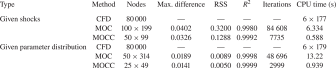
For further quantitative analysis, the results of a regression analysis of MOCC are presented in table 6. The CFD results are selected as the contrast data. First, focusing on the cases with given shocks, the table shows that the maximum difference and the RSS both decrease when using MOCC. As a result, the  $R^2$ value, which illustrates the goodness of fit, increases from 0.9980 to 0.9992. Statistically, the MOCC flowfield is more accurate than that of MOC. Furthermore, MOCC uses fewer nodes to acquire the more accurate solution. The number of iterations decreases by 90 % and the calculation only takes 0.588 s. The high accuracy-to-efficiency ratio persists in the flowfield calculation with a given parameter distribution. MOCC only uses
 $25 \times 49$ nodes to acquire a high-level similarity of 99.99 %. The calculation time decreases from 13.22 s with MOC to 0.939 s with MOCC. The efficiency increases by more than 90 %. For an optimization problem with one million cases, using MOCC would reduce the CPU time by 3411 h while maintaining a high level of accuracy. As for CFD, the CPU times for axisymmetric cases with given shocks and pressure distribution are
 $6\times 177$ s and
 $6\times 179$ s, respectively. The computational time of CFD can further decrease with techniques such as the adaptive mesh refinement. However, with a uniform grid and current model, using MOCC instead of CFD can save a significant amount of computing resources for the axisymmetric cases owing to the smaller number of grid nodes and simpler algorithm. Although CFD has wide generality, MOCC is a better choice for the inverse design in non-uniform flows because of its advantages in terms of accuracy and efficiency.
Regression analysis for MOCC in non-uniform flow.

4. Applications of MOCC in supersonic flowfield inverse design
4.1. Inverse design of the supersonic flowfield
As the high accuracy of MOCC in planar and axisymmetric flows has been verified in the previous section, MOCC can be applied to the inverse design of supersonic flowfields. An inlet design is logically separated into two sections: (1) determination of the inviscid supersonic flowfield; and (2) the inviscid inlet given by the stream-tracing technique. The first step is the core of the inlet design, because the performance is related to the supersonic flowfield. Thus, in this section, only the first step is studied. Considering its practical importance, the inverse design of supersonic flowfields is vital because the inlet performance is directly determined by the incident and reflected shocks (or outlet parameters). With given shocks or outlet parameters, the energy loss at the inviscid inlet can be calculated before generating the inlet. Note that only one condition (shocks or outlet parameters) is given as the boundary to avoid over-constraining the system. As the supersonic flowfield calculation is a mere repetition of unit processes, the inverse design is based on the three unit processes described in this paper. According to the different boundary conditions, the inverse design of supersonic flowfields is divided into three classes, as shown in figure 13. The first type is inverse design with an incident shock. This type is normally encountered in external flows. The second type is inverse design considering incident and reflected shocks, which is common in internal flows. The third type is inverse design with outlet parameters, because the outlet parameters are of vital importance in downstream areas. Detailed inverse schemes for these three classes are now illustrated in turn.
Inverse design of supersonic flowfields using MOCC. (a) Inverse design with incident shock, (b) inverse design with incident and reflected shocks and (c) inverse design with outlet parameters.

4.1.1. Inverse design with the incident shock
In an inviscid flow, the post-shock flow is an isentropic process. The total energy loss of the supersonic flow is determined by the incident shock. In terms of practical importance, the inverse design using the incident shock enables direct control of the aerodynamic performance. The inverse steps are illustrated for planar and axisymmetric flows. The shapes of the planar and axisymmetric incident shocks are given by the same quadratic curve,  $y=-0.1x^2-0.3x+1$. First, the R–H equations and curved shock equations are used to calculate the post-shock parameters and their gradients based on the incoming condition and the shock shape. With the boundary condition behind the shock, the interior process is then iterated along the streamwise direction to acquire converged aerodynamic parameters and their gradients. The solution domain is determined by the characteristic and streamline. The inverse-design results are shown in figure 14. Even with the same incident shock, the inverse-design planar and axisymmetric flowfields under different flow types are distinct. This phenomenon can be illustrated by the gradients. The analysis is presented in the next section.
Inverse design of planar and axisymmetric internal flowfields with the incident shock in uniform flow ( $y=-0.1x^2-0.3x+1$). (a) Planar flowfield and (b) axisymmetric flowfield.

4.1.2. Inverse design with incident and reflected shocks
Take the internal flow as an example. In an internal flow, the incident shock is generated when the incoming flow passes and deflects along the wall. The incident shock then impacts the centre-body and a reflected shock is created. As the total energy loss is determined by the incident and reflected shocks, the shapes of the incident and reflected shocks are given explicitly to directly control the aerodynamic performance. The internal flowfield design is decomposed into two parts, one considering the incident shock and the other handling the reflected shock. The incident shock part, known as the first part, is initially calculated to give the known conditions for the process of the second, reflected shock part. The planar and axisymmetric incident shocks are given by the same quadratic curve,  $y=-0.1x^2-0.3x+1$. The given shocks will be divided into several discrete segments. The R–H equations and curved shock equations are used to calculate the post-shock parameters and their gradients based on the incoming condition. For each segment, the interior process is iterated to acquire converged aerodynamic parameters and their gradients. The scheme is then applied along the flow direction to solve the incident shock part. The characteristics of the incident shock part are shown in figure 15(a,c). After calculating the incident shock part, the parameters along the characteristic provide the boundary condition of the reflected shock part. As the geometric equation of the reflected shock can be affected by the height of the centre-body, the reflected shock angles are given to define the shape. The flow direction behind the reflected shock is taken to be parallel to the
 $x$-coordinate. The shock process is used to solve for the parameters near the reflected shock, and the flow parameters in the region surrounded by the wall, reflected shock and characteristic are calculated using the interior process. The wall does not have a length restriction, and the solution stops at the intersection of the wall and the reflected shock. A centre-body is always set to avoid the Mach reflection, which would generate a subsonic area behind the Mach stem. This subsonic region degrades the aerodynamic performance of the basic flowfield. The solution domain can vary with the height of the centre-body. Next, once the parameters near the reflected shock have been acquired, the flowfield behind the reflected shock is solved through the interior process. For the test cases, the reflected shock angles change according to
 $\mathrm {d}\theta /\mathrm {d} x=-0.2$. The height of the centre-body is 0.25. The solved reflected shock part together with the incident shock part are shown in figure 15(b,d).
Inverse design of planar and axially symmetric internal flowfields with shocks in uniform flow ( $y=-0.1x^2-0.3x+1$). (a,b) Planar symmetric internal flowfields and (c,d) axially symmetric internal flowfields.

4.1.3. Inverse design with outlet parameters
In supersonic flows, although the incoming flow determines the downstream flowfield, an inverse method makes it possible to design the flowfield according to the outlet parameters. An inverse method with given outlet parameters is now developed to design the supersonic flowfield based on the outlet parameters. The outlet parameters behind the reflected shock in figure 15 are extracted as the boundary conditions. The given shock will be divided into several discrete segments. As the outlet parameters are known, the mass flow of each segment can be calculated. In the final chart of figure 13, every discrete point  $A_r$ on the reflected shock has a corresponding point
 $A_i$ on the incident shock. Based on the principle of flow conservation and the incoming condition, the height of
 $A_i$ can be determined. Additionally, on the basis of the outlet parameters, the total pressure before the reflected shock can be solved using the R–H equations. Because the total pressure is constant along the streamline according to the isentropic law, the total pressure behind the incident shock at
 $A_i$ is equal to the total pressure at
 $A_r$. According to the incoming condition, the shock angle of point
 $A_i$ is calculated using the R–H equations. The shock angle is then used to determine the abscissa value of point
 $A_i$. When all segments of the incident shock have been acquired, the shape of the incident shock is obtained, as shown in figure 16(a,c). The internal flowfield between the incident shock and the reflected shock can be decomposed into the incident shock part and the reflected shock part. The incident shock part is calculated using the interior process, with the scheme applied along the flow direction. Once the incident shock part has finished, the parameters along the characteristic are regarded as one of the boundary conditions for the calculation of the reflected shock part. Because the parameters near the reflected shock have already been acquired, the interior process can be applied to solve the aerodynamic parameters and their gradients in the flowfield surrounded by the wall, reflected shock and characteristic. The solved reflected shock part together with the incident shock part are shown in figure 16(b,d). Note that there is at most one solution for the inverse design with given outlet parameters.
Inverse design of planar and axially symmetric internal flowfields with outlet parameters in uniform flow. (a,b) Planar symmetric internal flowfields and (c,d) axially symmetric internal flowfields.

After determining the supersonic flowfield, the inlet can be generated using the stream-tracing technique. In some circumstances, a rectangular inlet entrance is designed for its ease of installation. To combine this with an elliptical combustor, an elliptical throat is required. The inverse design of the supersonic flowfield with outlet parameters has many merits in these situations, and is beneficial for the construction of the combustion process. With reasonable outlet parameters and shapes, the total pressure recovery can be determined before the generation of the inlet. The combustion performance can also be predetermined in the design process. Note that unreasonable outlet parameters and shapes will mean that the supersonic flowfield has no solutions. As the inviscid performance of the inlet has been determined, the generation of the inlet with the stream-tracing technique does not require optimization. The rectangular entrance can smoothly transition to an elliptical throat without sacrificing any aerodynamic performance. Although the upper surface is unpredictable and fixed by the inverse design with outlet parameters, it can still connect to the vehicle through a surrounding frame. Overall, the inverse design with outlet parameters offers a new perspective for the combined construction of the inlet and the combustion process.
4.2. Analysis of the inverse-design internal flowfield
4.2.1. Analysis of the internal flowfield
The flow characteristics of planar and axisymmetric flowfields with given shocks in a uniform flow can also be determined using MOCC, as shown in figure 15. From this figure, it is clear that the general flow patterns are similar, although the details of these two flowfields are different. In both flowfields, the Mach number decreases along the streamlines because they are both internal compressive flowfields. The incident shock waves impact at the point (1.6225, 0.25) and are reflected because of the flow deflection. The incident and reflected shock waves divide the whole flowfield into three parts: the incoming flow part, the middle part and the reflected post-shock part. The latter two parts are distinct for the planar and axisymmetric flowfields, even with the same given conditions. Obviously, the solution domain of the axisymmetric flowfield is larger than that of the planar flowfield. This interesting phenomenon is a result of different flow patterns. From the R–H equations, the post-shock aerodynamic parameters of planar and axially symmetric flowfields are the same for identical incident shock waves and incoming flow conditions. However, for planar flow, there is no curvature in the flow-normal plane of the shock wave, whereas the curvature of the shock wave in the flow-normal plane is non-zero for axisymmetric flow. Based on curved shock theory, the post-shock streamline curvature and pressure gradient are related to the curvature of the shock wave according to  $D_2=K_a S_a+K_b S_b$ and
 $P_2=J_a S_a+J_b S_b$. The coefficients
 $K_a$,
 $K_b$,
 $J_a$ and
 $J_b$ are functions of the pre- and post-shock aerodynamic parameters, and can be found in the paper by Mölder (Reference Mölder2016). Because the aerodynamic parameters and the shape of the incident shock are the same for the planar and axisymmetric flowfields, the coefficients
 $K_a$,
 $K_b$ and the streamwise curvature
 $S_a$ are also identical for these two flowfields. Therefore, the transverse curvature
 $S_b$ is the reason for the different streamline curvatures. Figure 17 shows the variation of these coefficients with respect to the streamline curvature and pressure gradient at Mach 6. The solid and dashed black curves denote the coefficients
 $K_a$ and
 $K_b$;
 $J_a$ and
 $J_b$ are represented by solid and dashed red curves, respectively. It is clear that
 $K_b$ is positive for the internal flow at an incoming Mach number of 6. According to the definition of
 $S_b=-cos(\theta _1)/y$, the transverse curvature is positive in the internal axisymmetric flow. Therefore, the streamline curvature of the axisymmetric flowfield is greater than that of the planar flowfield. However, as the values of the streamline curvature and flow deflection angle are negative, a larger streamline curvature corresponds to a slower change in the flow deflection angle. From the calculation using MOCC, this axisymmetric flow with a concave shock has a larger negative streamline curvature in both the region near the shock and the downstream area, which leads to a larger solution domain. The difference between the solution domains of the planar and axially symmetric flowfields under the same known conditions varies depending on the shock shape, incoming condition and flow pattern, but the analysis method is suitable for all situations.
Coefficients influencing the streamline curvature and pressure gradient ( $M=6$).

4.2.2. Analysis of the shock reflection in the inverse-design flowfield
MOCC is not only suitable for flowfield design, but is also applicable to flow analysis using the solved gradients. Shock reflection is a common phenomenon in the design of supersonic flowfields. Therefore, MOCC can be used to investigate the curved shock reflection of the supersonic flowfields discussed above. The reflection structure is of vital importance to the design of the supersonic flowfield, because the performance of the supersonic flowfield is closely related to the reflection structure. Although the Mach reflection is stabler than the regular reflection, the subsonic area behind the Mach reflection has a negative effect on the aerodynamic performance. To avoid the Mach reflection, a centre-body is always set in the flowfield. Therefore, the polar lines around the reflected point can be used to investigate the relation between the centre-body and the shock reflection. For comparison, a series of flowfields with different centre-body heights are determined using MOCC. The resulting planar and axisymmetric flowfields are shown in figures 18(a) and 18(b), respectively. The horizontal coordinate is the flow deflection angle and the longitudinal coordinate is the static pressure ratio. In this figure, the flow angle towards the centre-body is regarded as positive. The incoming pressure is chosen as the reference value for dimensionless treatment. In both figures, the solid red curves indicate the incident shock, whereas the dashed red curves represent the reflected shock. The blue solid curves indicate the derivative of the post-shock pressure with respect to the flow deflection angle, which is referred to as the ‘polar streamline’ by Mölder (Reference Mölder1972). The polar streamline has the advantage of determining the reflection structure. In the ( $p$–
 $\delta$)-plane, Mölder (Reference Mölder1972) gave the expression of the polar streamline as
 $\mathrm {d} p/ (\rho V^2 \, \mathrm {d} \delta ) = P/ D$. Similarly, in the (
 $\ln (p)$–
 $\delta$)-plane, the polar streamline is expressed as
 $\mathrm {d} (\ln (p/p_0))/ \mathrm {d} \delta = (\gamma M^2 P)/ D$. As the pressure and flow direction remain the same on both sides of the slip layer (von Neumann Reference von Neumann1943), their gradients should also be fixed along the slip layer. Thus, the slope of the polar streamline (which is a function of the pressure, its gradient and the streamline curvature) must be identical on both sides of the slip layer. As a result, the slope of the polar streamline from the reflected shock polar can be used to calculate the parameters and their gradients behind the Mach stem. The calculation can be reversed when the condition behind the Mach stem is known.
Shock polar and polar streamline with given shocks in planar and axisymmetric flow ( $y=-0.1x^2-0.3x+1$). (a) Planar shock polar and polar streamline and (b) axisymmetric shock polar and polar streamline.

The flow pattern around the reflected point can be illustrated in the  $\ln (p)$–
 $\delta$ plane. In figure 18, point 1 denotes the incoming flow, before the incident shock deflects the flow to point 2 and the reflected shock is generated to deflect the flow back to the horizontal condition. For a curved incident shock, point 2 is in a different position depending on the height of the centre-body. When the centre-body changes, the incident shock angle also varies, which leads to a different deflection angle. For these calculated flowfields, point 2 moves up and to the right along the solid red curve as the height of the centre-body decreases. For each centre-body height, there is a corresponding Mach number behind the incident shock at the reflected point. The reflected shock polar is drawn on the basis of this post-shock Mach number. For regular reflections, the flow state behind the reflected shock is denoted by point 3.
Comparing the planar and axisymmetric flowfields, it is apparent that the solid red curves are exactly the same for both flowfields, as are the dashed red curves. This is because the shock polar is a function of the shock angle and the pre-shock condition. For both flowfields, the given conditions are identical. Therefore, the incident and reflected shock polar lines have the same variations at a certain centre-body height. However, this does not mean that the planar flow structure around the reflected point is the same as in the axisymmetric flowfield, because the aerodynamic variables only determine the flow state at some certain point. Rather, the gradients of those parameters determine the flow pattern in a certain area. There is an obvious contrast between the polar streamlines of the planar and axisymmetric flows. For the planar incident shock, figure 18(a) shows that the incident slope of the polar streamline is negative and barely changes for all centre-body heights. The reason is that only streamwise curvature exists in the planar flow. Thus, the incident slope of the polar streamline can be simplified as follows:
 \begin{equation} \frac{\mathrm{d} (\ln(p/p_0))}{ \mathrm{d} \delta} = \frac{\gamma M^2 P}{ D} = \frac{\gamma M^2 J_a}{K_a}. \end{equation}
Obviously, the slope of the polar streamline behind the incident shock is irrelevant to the curvature. From figure 17, it can be seen that the variables  $J_a$ and
 $K_a$ are positive and negative, respectively, but have similar variations in this internal planar flowfield. As a result, the incident slope of the polar streamline remains almost constant at a finite negative value as the height of the centre-body increases. Specifically, the streamline curvature is negative and the pressure gradient is positive in this planar flowfield, and so regardless of where the reflection happens, behind the incident shock, the pressure increases along the streamline while the streamline deflects toward the centre-body. By contrast, the incident slope of the polar streamline varies with the height of the centre-body in the axisymmetric flow. As the height of the centre-body decreases, the incident slope changes from negative to positive, and then back to negative. The transverse curvature is the reason for this behaviour. The expression of the polar streamline for the axisymmetric flow is as follows:
 \begin{equation} \frac{\mathrm{d} (\ln(p/p_0))}{ \mathrm{d} \delta} = \frac{\gamma M^2 P}{D} = \gamma M^2\frac{ J_a S_a+J_b S_b}{ K_a S_a+K_b S_b}. \end{equation}
The curvature cannot be removed. The slope of the polar streamline behind the axisymmetric incident shock is related to the shock curvature and the incoming flow. The first transformation from negative to positive occurs at the Crocco point ( $h=0.37$), where the incident post-shock streamline curvature is zero, and the second transformation takes place at the Thomas point, where the incident post-shock pressure gradient is zero. Furthermore, as the height of the centre-body approaches zero, the transverse curvature approaches infinity, which results in an infinite pressure gradient and streamline curvature. Rylov (Reference Rylov1990) has verified that, for this situation, the regular reflection cannot exist. A Mach stem is generated to keep the flow parallel to the level behind the shock. Thus, although the reflected shock polar of the axisymmetric flowfield without a centre-body is the same as the planar reflected shock polar and has an intersection with the line
 $x=0$, the regular reflected point is a non-physical solution. Only irregular reflection can occur in the axisymmetric flow without a centre-body. In the presence of a centre-body, its height determines whether the Mach reflection is able to form. Based on the von Neumann criterion (Ben-Dor Reference Ben-Dor2007), when the reflected shock polar has only one intersection with the incident shock polar, the Mach reflection cannot be formed. For instance, the reflected shock polar lines for the planar and axisymmetric flowfields are shown for a centre-body height of 0.6. There is only one interaction between the incident and reflected shock polar lines. Thus, only regular reflection can exist in either flowfield with this centre-body. When the centre-body height is less than 0.45, both regular and irregular reflections are able to form. Therefore, for this test case, the centre-body height should be greater than 0.45 to completely avoid the formation of the Mach reflection in planar and axisymmetric flows. Note that the demarcation height varies with the shock shape and incoming flow condition.
Focusing on the reflected shock polar (red dashed curves), these curves can also be regarded as the relation between the reflected post-shock pressure and the flow deflection angle under the same pre-shock condition. Take the planar case with a centre-body height of 0.25 as an example. As the angle between the reflected post-shock flow angle and the  $x$-coordinate decreases from zero, the reflected shock needs to be stronger to increase the deflection angle. Thus, the post-shock pressure also rises to match the stronger shock wave. However, unlike the incident slope of the polar streamline, the reflected slope varies with the flow deflection angle because it is related to the curvatures. As above, the incident slope of the planar polar streamline is irrelevant to the incident shock curvature, because the streamline-wise curvature can be removed in the slope expression. For the planar reflected shock, however, the post-shock pressure gradient and the streamline curvature are related to both the reflected and incident shock curvatures. These curvatures cannot be eliminated from the reflected slope expression. Therefore, the reflected slope changes from positive to negative as the flow deflection angle decreases. The turning point is the reflected Crocco point. Furthermore, the flow deflection angle at the reflected Crocco point decreases as the centre-body height increases. For the axisymmetric flow, the reflected shock polar is identical to the planar one with the same centre-body height because the reflected pre-shock aerodynamic parameters are consistent. Similarly, the slope of the reflected polar streamline in the axisymmetric flow is related to the incident and reflected shock curvatures. Unlike the case of planar regular reflection, both the Crocco point and the Thomas point exist. However, the existence of the reflected Thomas point is dependent on the centre-body height in the axisymmetric flow. For example, the reflected Thomas point exists in the axisymmetric internal flowfield with a centre-body height of 0.25, but does not exist when the centre-body height is 0.6.
5. Conclusions
The proposed MOCC expands the application range of curved shock theory by determining the gradients in the supersonic flowfield. In this paper, explicit expressions for MOCC have been obtained in total differential form. MOCC has been applied to solve supersonic flowfields in planar/axisymmetric, external/internal and uniform/non-uniform flows. The results show that, owing to the use of gradients, MOCC can obtain explicit supersonic flowfields with fewer nodes than MOC. MOCC not only achieves a high degree of accuracy, but also reduces the computational load by around 80 % compared with the conventional MOC. As with MOC, the proposed MOCC can be applied to the inverse design of supersonic flowfields, such as designs with shocks or outlet parameters. However, MOCC achieves better accuracy and efficiency in the inverse design. Furthermore, the gradients determined by MOCC are applicable to the shock reflection area in planar and axisymmetric flows. For the test cases reported herein, the shock polar and polar streamlines acquired from MOCC show that both the Crocco point and the Thomas point can exist in axisymmetric regular reflection, whereas only the Crocco point can form in the planar regular reflection. As the gradients approach infinity, it becomes impossible for regular shock reflection to occur. The gradients used to describe the flow tendency make MOCC a good candidate for flow analysis and the inverse design of supersonic flowfields.
Mölder and Emanuel have pointed out that the curved shock theory is applicable to three-dimensional flows, but the flow plane should be identical to the osculating plane (Mölder Reference Mölder2016). Similarly, MOCC can be applied to three-dimensional flows when there are no lateral gradients, such as the symmetry plane of an elliptic flowfield. However, for the extension of MOCC to general three-dimensional supersonic flow, the governing equation needs to be derived from the three-dimensional Euler equation. Furthermore, three-dimensional curved shock equations are required to determine the gradients behind a three-dimensional curved shock. It is likely that the three-dimensional governing equations will become more complex as the number of variables increases. However, it will be worth developing the three-dimensional curved shock theory considering the theoretical value and wide application range. In addition, because Li et al. (Reference Li, Shi, Zheng and You2019) and Zheng et al. (Reference Zheng, Hu, Li, Zhu, You and Song2020) successfully solved the three-dimensional post-shock flowfield based on two-dimensional MOC, MOCC also has the potential to be applied in three-dimensional flows efficiently and accurately.
Funding
We wold like to acknowledge the support of the National Natural Science Foundation of China (NSFC, grant nos. 91941103 and u20A2069) and the Aeronautical Science Foundation of China (ASFC, grant no. 2018ZB68008).
Declaration of interests
The authors report no conflict of interest.