1 Introduction
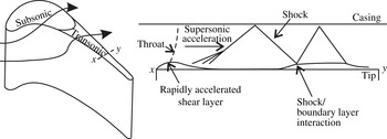
Here, we present direct numerical simulations (DNS) of a transonic turbine tip flow with free-stream disturbances at engine representative Mach and Reynolds numbers in order to determine the effects of turbulence on the tip heat transfer and aerodynamics. Turbine blade tips can experience significant degradation throughout the engine life cycle due to the high mechanical and thermal stresses in the tip region. The high thermal loads are largely due to the tip leakage flow, which forms in the gap between the moving rotor blade tips and the casing of the machine. Turbine tip flows are also responsible for up to 30 % of stage losses for newly installed engines (Harvey Reference Harvey2004). In service, the blade tips are eroded due to chemical attack, fatigue and creep, which are all exacerbated by the high gas temperatures, and this causes further performance degradation (Bunker Reference Bunker2004). Prediction of the correct heat transfer to the tip is consequently a critical part of the turbine design process. Shroudless high-pressure (HP) turbine blades can have peak Mach numbers within the tip gap of 1.8 and, thus, supersonic effects cannot generally be ignored (Moore et al. Reference Moore, Moore, Henry and Chaudhry1989; Moore & Elward Reference Moore and Elward1993; Wheeler, Atkins & He Reference Wheeler, Atkins and He2011; Zhang et al. Reference Zhang, O’Dowd, He, Wheeler, Ligrani and Cheong2011). Supersonic effects tend to occur over the aft region of the tip where the blade loading is highest, although the extent of supersonic flow over the tip is strongly dependent on the tip geometry (Coull, Atkins & Hodson Reference Coull, Atkins and Hodson2014; Zhang, He & Rawlinson Reference Zhang, He and Rawlinson2014). This area of the tip is important because the blade thickness in this region is small, which means that complex tip geometries are often not feasible and this zone is typically difficult to cool. The basic tip flow structure in this region is shown in figure 1. As the flow enters the tip gap, the flow separates from the pressure side corner. The separation accelerates the flow to supersonic conditions like a converging–diverging nozzle; thus, as the separation begins to reattach, the change in area forces the mainstream flow to accelerate. This in turn aids the reattachment (Wheeler et al. Reference Wheeler, Atkins and He2011). Compression waves form due to the curvature of the reattaching boundary layer. These coalesce into an oblique shock which reflects from the tip and casing, leading to shock/boundary layer interactions which can cause further boundary layer separation. The reattachment process of the separation bubble at the inlet to the gap is important because it will influence the heat transfer over the remainder of the tip. From extensive data on subsonic tip flows it is known that high levels of turbulent mixing in the reattachment zone lead to high heat transfer levels downstream of the separation bubble (Bunker Reference Bunker2004). However, the extent to which heat transfer levels are diminished when the separation bubble reattachment occurs through supersonic acceleration has not yet been reported in detail, although the results of Zhang & He (Reference Zhang and He2013), De Maesschalck, Lavagnoli & Paniagua (Reference De Maesschalck, Lavagnoli and Paniagua2014) and De Maesschalck, Lavagnoli & Paniagua (Reference De Maesschalck, Lavagnoli and Paniagua2015) do suggest that this supersonic acceleration can be exploited to reduce tip heat load. Wheeler & Sandberg (Reference Wheeler and Sandberg2012) recently presented DNS results showing the intermittent nature of the transonic tip flow, fluctuating between laminar and turbulent flow downstream of the bubble reattachment.
Schematic of a transonic tip flow.

The effects of turbulence on tip heat transfer are likely to be important, but it is interesting to note that although Mach numbers are high in the tip gap, the Reynolds number of the tip flow will generally be low (based on gap height,
 $g$
,
 $Re_{g}\sim 2\times 10^{4}$
). The low Reynolds number and the presence of strong accelerating pressure gradients downstream of the separation raises the possibility that the transonic tip flow may not be fully turbulent. This is important because the ability of turbulence models to cope with transitional flows is questionable, and so this raises questions about the use of Reynolds-averaged Navier–Stokes (RANS) methods for the prediction of blade tip heat transfer.
This paper aims to use DNS to solve the turbulent unsteadiness and therefore fully resolve the boundary layer flow on the tip. The objective is to determine the sensitivity of the tip flow to incoming disturbances. In order to more accurately represent the actual flow configuration of a high-pressure turbine tip gap, cross-flow and a pressure surface boundary layer were also included in the simulations. The flow is simulated over an idealized tip geometry where the tip gap is represented by a constant-area channel with a sharp inlet corner to represent the pressure side edge of the turbine blade. The paper is structured as follows. The compressible code used in this study is introduced in § 2. The set-up of an engine representative tip flow and grid sensitivity are described in § 3. In § 4, DNS results, linear stability analysis and Reynolds number dependence are presented for the datum case. This is followed by an investigation of the effects of free-stream disturbances, cross-flow and pressure surface boundary layer on the tip heat transfer and skin friction in § 5. The paper concludes with a discussion of the most important results in § 6.
2 Solution algorithm and data processing
The DNS were performed with an in-house multiblock structured compressible Navier–Stokes solver purposely developed for exploiting high-performance computing systems. The numerical method comprises a five-step fourth-order-accurate low-storage Runge–Kutta method (Kennedy, Carpenter & Lewis Reference Kennedy, Carpenter and Lewis2000), with a Fourier method for discretization of the spanwise direction. Spatial derivatives in the streamwise and lateral directions are discretized using a central fourth-order-accurate finite-difference scheme with energy conserving boundary schemes of the same formal order (Carpenter, Nordstrm & Gottlieb Reference Carpenter, Nordstrm and Gottlieb1999). Additionally, a skew-symmetric splitting (Kennedy & Gruber Reference Kennedy and Gruber2008) is used to stabilize the convective terms. The code has been validated against a number of benchmark cases and used, among other applications, for DNS of supersonic axisymmetric wakes (Sandberg Reference Sandberg2012) and turbulent jets in coflow (Sandberg, Sandham & Suponitsky Reference Sandberg, Sandham and Suponitsky2012). More recently, the code has also been applied to low-pressure turbine flows (Sandberg et al. Reference Sandberg, Pichler, Chen, Johnstone and Michelassi2015), transonic tip flows (Wheeler & Sandberg Reference Wheeler and Sandberg2012) and high-pressure transonic turbine flows (Wheeler et al. Reference Wheeler, Sandberg, Sandham, Pichler, Michelassi and Laskowski2016).
The surface heat flux is presented as a normalized heat flux defined as
 $$\begin{eqnarray}q_{norm}=\frac{qg}{(T_{o}-T_{w})k_{ref}},\end{eqnarray}$$
where
 $q$
is the surface heat flux,
 $T_{o}$
is the free-stream stagnation temperature,
 $T_{w}$
is the wall temperature and
 $k_{ref}$
is a reference conductivity, taken to be at the gap exit static temperature in the free stream. Some results presented are shown in terms of the isentropic Mach number, which is the Mach number determined from the local surface static pressure and inlet total pressure. The heat transfer coefficient (
 $h$
) is determined by performing simulations at two wall temperatures (
 $T_{w}/T_{o}=1.03$
and 0.89) and calculating the difference in local heat transfer at the two different wall temperatures (i.e.
 $h=\unicode[STIX]{x0394}q/\unicode[STIX]{x0394}T_{w}$
). The heat transfer coefficient is presented in this paper as a Nusselt number, consistent with the definition of Reynolds number,
 $$\begin{eqnarray}Nu=\frac{hg}{k_{ref}}.\end{eqnarray}$$
Results for skin friction are also shown and these are determined using the local time-averaged wall shear stress and the local boundary layer edge velocity and density. All quantities presented in this paper are non-dimensionalized based on reference conditions at the gap exit and a length scale equal to the gap height (
 $g$
). Velocities are therefore normalized by the free-stream velocity at the gap exit (
 $u_{ref}$
), the turbulent kinetic energy is normalized by
 $u_{ref}^{2}$
and the vorticity is normalized by
 $u_{ref}/g$
. Time is normalized by
 $g/u_{ref}$
and thus one unit represents the time taken for the flow to pass through a length equal to the height of the gap. Likewise, the frequency
 $f$
is given as a non-dimensional quantity, using the reference velocity and gap height to non-dimensionalize. The power spectral density of the velocity magnitude,
 $P_{xx}$
, is normalized by
 $u_{ref}^{2}$
. The Reynolds number is defined based on these reference conditions as
 $Re_{g}=\unicode[STIX]{x1D70C}_{ref}u_{ref}g/\unicode[STIX]{x1D707}_{ref}$
, where
 $\unicode[STIX]{x1D70C}_{ref}$
and
 $\unicode[STIX]{x1D707}_{ref}$
are the density and viscosity at the reference condition, respectively. For the cases with cross-flow, the Reynolds number is based on the free-stream velocity magnitude at the gap exit,
 $Re_{g}=\unicode[STIX]{x1D70C}_{ref}\sqrt{u_{ref}^{2}+w_{ref}^{2}}g/\unicode[STIX]{x1D707}_{ref}$
. Since, for the cross-flow cases, the spanwise component of the velocity was
 $w_{ref}=0.25u_{ref}$
the Reynolds number based on the
 $x$
component of velocity was 4 % lower than the cases without cross-flow.
Statistical quantities were determined using long time series data to ensure convergence of the statistical quantities. By comparing the statistics obtained over a number of subsequent time intervals with each other it was found that statistical convergence was obtained using long time series data over a non-dimensional time of
 $\unicode[STIX]{x0394}t=50$
. During the solutions, Favre-based time integration was used to determine the time-averaged flow field and turbulence quantities.
3 Numerical set-up of an engine-scale tip flow
Direct numerical simulations were performed at Reynolds numbers of
 $1\times 10^{4}\leqslant Re_{g}\leqslant 2\times 10^{4}$
, based on gap exit conditions and gap height. Typical HP blade Reynolds numbers based on blade exit conditions are approximately
 $1{-}2\times 10^{6}$
, with gap heights in the range of 1 % span. The tip gap Reynolds number in this study is thus in the engine representative range for low-aspect-ratio blading; DNS predictions of the effect of tip gap Reynolds number were discussed previously by the authors in Wheeler & Sandberg (Reference Wheeler and Sandberg2012).
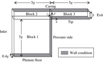
A schematic of the computational domain is shown in figure 2. The flow is simulated over an idealized tip geometry. In this geometry, the tip gap is represented by a constant-area channel with a sharp inlet corner to represent the pressure side edge of the turbine blade. This representation of a turbine tip flow has been used several times in previous work (for instance, see Chen, Dawes & Hodson (Reference Chen, Dawes and Hodson1993)). An example of a typical flow pattern is shown in figure 3. The flow separates at the sharp inlet edge causing the characteristic separation bubble found in most tip gap flows. The formation of shock waves is typical of the tip gap flows found in transonic blade rows (for example Moore & Elward Reference Moore and Elward1993; Wheeler et al.
Reference Wheeler, Atkins and He2011; Zhang et al.
Reference Zhang, O’Dowd, He, Wheeler, Ligrani and Cheong2011). A tip width-to-gap ratio of 5 was chosen, which is similar to the tip geometry near the blade trailing edge. This region was chosen because here accurate prediction of the physical mechanisms of the flow and the heat transfer is particularly important for the above mentioned reasons. The upstream plenum dimensions in the
 $x$
and
 $y$
directions were chosen to be
 $5g$
and
 $6g$
respectively. The effect of plenum size was tested with steady RANS simulations using the FLUENT v16.0 density-based second-order solver, with a Spalart–Allmaras turbulence model; increasing the plenum size from
 $5\times 6g$
to
 $10\times 11g$
was found to have minimal effects on the flow structures in the tip gap, such as shock positions and separation bubble size.
The computational domain.

An example of the simulated flow field with turbulent inflow. Contours of vorticity magnitude and isosurface of vorticity magnitude (
 $\unicode[STIX]{x1D714}=5$
).

Characteristic boundary conditions were applied at the exit to avoid reflections from this boundary. A zonal characteristic boundary condition (Sandberg & Sandham Reference Sandberg and Sandham2006) was applied over the final 50 streamwise grid lines, i.e. to the last
 $0.25g$
of the computational domain, which has previously been shown to be highly effective in attenuating acoustic reflections from vortical structures passing through the outlet boundary. The solid boundary on the ‘casing’ was treated as a slip wall since simulation of the boundary layer on the casing was not part of this investigation; the influence of the casing with relative motion between the blade tip and the casing wall is a subject for future investigation. The effect of casing shear on the tip flow was the subject of a recent experimental investigation in a rotating transonic high-pressure turbine by Jackson, Wheeler & Ainsworth (Reference Jackson, Wheeler and Ainsworth2015). In the study of Jackson et al. (Reference Jackson, Wheeler and Ainsworth2015), experimental results were compared with computational simulations where a no-slip wall and a slip wall were imposed on the casing. The effect of casing shear was to change the tip surface adiabatic wall temperature due to the effect of casing shear on the relative total temperature in the tip gap. Nonetheless, the flow field was qualitatively similar to cases without casing shear, in terms of the general flow structure and reattachment point heat transfer levels. For the present study it was decided to model the casing as a slip wall; this avoided the non-trivial task of imposing a mixed inflow/outflow boundary at the gap exit (since the moving wall drags the endwall boundary layer into the gap). Furthermore, the nature of the endwall boundary layer adds several more uncertainties which were beyond the scope of this study (aspects such as boundary layer skew, thermal profile of the boundary layer). Inclusion of the endwall boundary layer would have been further complicated by the fact that the state of the endwall boundary layer in an engine environment has so far not been widely reported, and a ‘correct’ representation of this in itself is something beyond the scope of this study.
The tip surface was treated as a non-slip isothermal boundary. It should be noted that for non-adiabatic computational fluid dynamics (CFD) calculations it is common to use an isothermal wall condition, as done in this study, although the true wall temperature will depend on the heat transfer to the solid as well as the fluid, which requires a conjugate analysis. The Nusselt number, however, is normally considered to be independent of the wall temperature (provided that the wall temperature is not greatly varying). The solid walls in the upstream blocks were treated as slip walls apart from the vertical face on the right in block 1 (see figure 2). This wall represents the pressure side surface of the blade and was treated as either a slip or a no-slip wall depending on the test case, as discussed later. The additional slip wall case was considered in order to determine the importance of the pressure side boundary layer in affecting the global tip gap flow. This was particularly important as it was felt that accurately representing the boundary layer characteristics of a full turbine configuration would be challenging at best.
The inlet flow was prescribed using the following relationships for the
 $u$
,
 $v$
and
 $w$
components of velocity:
 $$\begin{eqnarray}\displaystyle u & = & \displaystyle u_{in}+\frac{4}{\unicode[STIX]{x03C0}}A\left(\cos (\unicode[STIX]{x1D703}_{y})-\frac{\cos (3\unicode[STIX]{x1D703}_{y})}{3}+\frac{\cos (5\unicode[STIX]{x1D703}_{y})}{5}-\frac{\cos (7\unicode[STIX]{x1D703}_{y})}{7}\right)\nonumber\\ \displaystyle & & \displaystyle \times \left(\cos (\unicode[STIX]{x1D703}_{z})-\frac{\cos (3\unicode[STIX]{x1D703}_{z})}{3}+\frac{\cos (5\unicode[STIX]{x1D703}_{z})}{5}-\frac{\cos (7\unicode[STIX]{x1D703}_{z})}{7}\right),\end{eqnarray}$$
 $$\begin{eqnarray}\displaystyle & v=A\sin (\unicode[STIX]{x1D703}_{z})\cos (\unicode[STIX]{x1D703}_{y})\sin (2\unicode[STIX]{x03C0}tu/l), & \displaystyle\end{eqnarray}$$
 $$\begin{eqnarray}\displaystyle & w=w_{in}+A\cos (\unicode[STIX]{x1D703}_{z})\sin (\unicode[STIX]{x1D703}_{y})\sin (2\unicode[STIX]{x03C0}tu/l), & \displaystyle\end{eqnarray}$$
where
 $u_{in}$
and
 $w_{in}$
are the spatial averages of the
 $u$
and
 $w$
components of the velocity over the inlet;
 $\unicode[STIX]{x1D703}_{y}=2\unicode[STIX]{x03C0}y/l$
;
 $\unicode[STIX]{x1D703}_{z}=2\unicode[STIX]{x03C0}z/l$
. The length scale was
 $l=0.2g$
, and the amplitude
 $A$
was 0, 2.0 or 4.0 depending on the case. This method approximates the flow downstream of a perforated sheet by producing a spatial ‘chessboard’ pattern in the
 $u$
velocity, and temporal fluctuations in
 $v$
and
 $w$
which simulate streamwise vortices convecting at the local velocity, while remaining divergence free.
These equations were used to generate deterministic perturbations at the inflow at low computational cost (other methods can be used but can be computationally expensive). This set of equations provided a way of generating fluctuations over a range of scales that stability analyses (shown later) suggested the tip flow shear layer would be sensitive to. Figure 3 shows an example flow field with this inlet disturbance specification; it is interesting to note the large attenuation of turbulence and stretching of the vorticity field as the flow accelerates into the tip gap.
The turbulence levels and length scales in the real turbine environment are not well known, especially near the endwalls where turbulence will arise from a wide range of sources such as endwall boundary layers, secondary flows and stator–rotor interactions. Thus, the results presented in this paper give an indication of the turbulent flow within the tip gap when subjected to turbulence at high and low intensity, albeit with length scales of a similar order of magnitude to the tip gap.
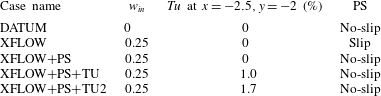
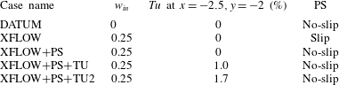
Case details.
3.1 Overview of test cases
A number of test cases were simulated to determine the sensitivity of the tip flow to free-stream disturbance, cross-flow and the pressure side boundary layer (see table 1). The ‘DATUM’ case simulates a tip flow without cross-flow and with a clean inflow, i.e. with no free-stream disturbances or pressure surface boundary layer. The cases with cross-flow (‘XFLOW’) all had a cross-flow of 25 % of the tip gap exit velocity. In an actual turbine tip flow, the ratio of cross-flow velocity to gap exit velocity will largely be determined by the ratio of the pressure side and suction side velocities (since the gap exit velocity will be similar to the local suction side velocity and the cross-flow velocity will be set by the local pressure side velocity). A value for this ratio of approximately 0.25 is thus representative of a tip flow exiting near to peak suction. The ‘XFLOW’ and ‘XFLOW
 $+$
PS’ cases both have zero-amplitude inlet free-stream disturbances. However, while the ‘XFLOW’ case sets a slip wall for the pressure surface (PS), the ‘XFLOW
 $+$
PS’ simulates the effect of a pressure surface boundary layer by including the pressure surface (PS) as a no-slip wall. The introduction of cross-flow makes it possible to test the effect of the pressure side boundary layer on the tip gap flow. The cases with a slip wall and with no-slip on the pressure side wall are compared with each other in this study in order to determine whether the pressure side boundary layer plays a significant role in the stability of the tip surface boundary layer and separation.
The other two cases, ‘XFLOW
 $+$
PS
 $+$
TU’ and ‘XFLOW
 $+$
PS
 $+$
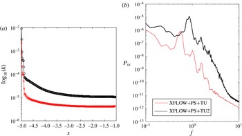
TU2’, include two levels of inflow disturbances, generated by the method discussed above. For these two cases, wave amplitudes of 16 % and 32 % are prescribed at the inlet respectively. Figure 4(a) shows the variation in turbulent kinetic energy within the plenum, averaged over the plenum height; there is a rapid reduction in turbulent kinetic energy over the first 10 grid points where high-frequency energy is dissipated due to the non-physical nature of the introduced flow perturbations and filtering (since the square-wave approach we use introduces both high- and low-frequency content). Further downstream, there is a more gradual reduction in turbulent kinetic energy, due to a combination of having relatively low speed and thus low-Reynolds-number flow upstream of the gap, with high viscous dissipation, and very strong acceleration when entering the gap. This means that the turbulence intensity at the inlet to the tip gap drops to below 1 % despite the very high levels upstream. In table 1 we therefore quote the turbulence intensity at the centre of the plenum.
Variation of the turbulent kinetic energy with distance upstream of the tip gap (a); power spectra of the velocity magnitude at the gap inlet
 $x=0.0$
,
 $y=0.7$
for two inlet disturbance levels (b).

The experimental results of Zhang et al. (Reference Zhang, He and Rawlinson2014) in a transonic turbine cascade have previously shown that the tip heat transfer is insensitive to changes in turbulence intensities from 1 %–9 %, and this is probably a result of the observed attenuation of free-stream turbulence seen here. Power spectra of the free-stream disturbances at the inlet to the tip gap are shown in figure 4; the unsteadiness is largely distributed at low frequencies, and this is a result of specifying a relatively large length scale for the inlet disturbances (
 $l=0.2$
), as described earlier.
3.2 Grid sensitivity
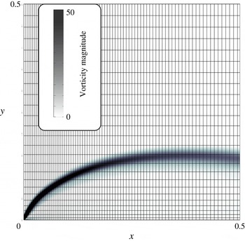
Figure 5 shows the computational mesh in the region of the inlet corner. Contours of vorticity magnitude are shown to indicate the shear layer of the separation bubble. The near-wall grid spacings in the
 $x$
,
 $y$
and
 $z$
directions were typically on average
 $y^{+}=0.4$
,
 $x^{+}=2$
and
 $z^{+}=4$
over the tip surface for the case with 16 modes and a spanwise extent of
 $0.4g$
. A mesh sensitivity study was performed at the datum conditions of
 $Re_{g}=20K$
,
 $w_{in}=0$
,
 $A=0$
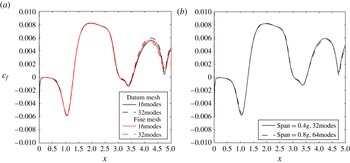
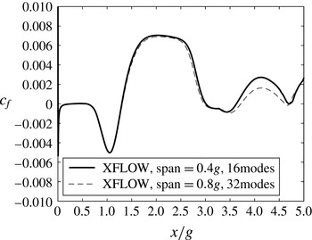
. Figure 6(a) shows time- and spanwise-averaged results of skin friction from three-dimensional (3D) calculations using the datum grid with a spanwise extent of
 $0.4g$
, and results using a finer grid which had a 50 % increase in grid points in each direction in physical space (thus having over twice as many cells as the datum grid in the
 $x{-}y$
plane). The ‘datum’ mesh used here had 200 points across the height of the gap (in the
 $y$
direction), and 1000 points across the width of the gap (in the
 $x$
direction). Within the upstream plenum there were 400 points in the
 $x$
direction and 400 points in the
 $y$
direction. Results using either 16 or 32 Fourier modes across the span are also shown in figure 6(a). Data downstream of
 $4.75g$
should be ignored because this is within the region of the zonal characteristic boundary condition. The figure shows little difference between the solutions over the majority of the tip (
 ${\sim}1\,\%$
), especially upstream of
 $3.5g$
. The region of sensitivity downstream of
 $3.5g$
is due to the influence of a shock/boundary layer interaction in this region, as will become evident later in the paper. The difference in predicted skin friction between the datum grid with 16 spanwise modes and the fine grid with 32 spanwise modes peaks at approximately 10 % within this region. The choice of at least 16 modes across a span of
 $0.4g$
ensured that spanwise variations in the flow were adequately captured (i.e. there was at least a 100-fold reduction in the amplitude of the Fourier modes from the first to the 16th mode). The span is kept small in order to allow for a higher grid resolution in the spanwise direction. In figure 6(b), skin friction results are compared for two cases with different spanwise extents (
 $0.4g$
and
 $0.8g$
). For these two cases, the number of modes per unit spanwise distance is preserved, i.e. the number of modes is doubled from 32 to 64 when the spanwise extent is increased from
 $0.4g$
to
 $0.8g$
. It can be seen that the wider domain has an almost negligible influence on the skin friction (see figure 6
b). As will be shown in the section on stability analysis (§ 4.1), a width of
 $0.4g$
is sufficient to capture the most unstable spanwise modes that lead to breakdown to turbulence for the datum case.
Computational mesh in the region of the separation bubble, showing only every fourth grid line.

Skin friction predictions for different grid sizes and spanwise extents.

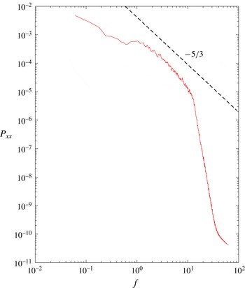
Fourier spectra within the boundary layer showed that fluctuations in turbulent kinetic energy are captured over five orders of magnitude using this datum mesh (see figure 7). It is interesting to note at this point the departure of the spectrum from the
 $-5/3$
slope characteristic of isotropic turbulence. Although this will be discussed in more detail later, it is useful to bear in mind that the tip flow does not undergo a complete transition to fully turbulent flow.
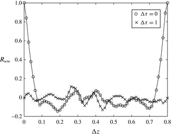
The autocorrelation function for the spanwise velocity component is given in (3.4), and this can be used to estimate the decorrelation of the flow with time and spanwise distance:
 $$\begin{eqnarray}R_{ww}(\unicode[STIX]{x0394}\unicode[STIX]{x1D70F},\unicode[STIX]{x0394}z)=\frac{\displaystyle \int _{0}^{\infty }w^{\prime }(t,z)w^{\prime }(t+\unicode[STIX]{x0394}\unicode[STIX]{x1D70F},z+\unicode[STIX]{x0394}z)\,\text{d}t}{\displaystyle \int _{0}^{\infty }w^{\prime }(t,z)^{2}\,\text{d}t}.\end{eqnarray}$$
Figure 8 shows the variation of the autocorrelation function of the spanwise velocity component
 $R_{ww}(\unicode[STIX]{x0394}\unicode[STIX]{x1D70F},\unicode[STIX]{x0394}z)$
with spanwise distance at two phase differences (
 $\unicode[STIX]{x0394}\unicode[STIX]{x1D70F}=0$
and 1). As expected, over large time shifts the flow becomes decorrelated from an initial state, as indicated by the low values of the autocorrelation function at
 $\unicode[STIX]{x0394}\unicode[STIX]{x1D70F}=1$
. For the case when
 $\unicode[STIX]{x0394}\unicode[STIX]{x1D70F}=0$
, decorrelation occurs over spanwise distances greater than
 $0.1g$
, and this is further verification of the choice of
 $0.4g$
as an appropriate spanwise extent for the DNS study conducted here.
Power spectrum of the velocity magnitude at
 $x=4.2$
,
 $y=0.1$
(
 $w_{in}=0$
,
 $A=0$
,
 $\text{span}=0.4g$
).

Autocorrelation function of the spanwise velocity
 $w^{\prime }$
at
 $x=4.2$
,
 $y=0.1$
(
 $w_{in}=0$
,
 $A=0$
,
 $\text{span}=0.8g$
, 32 spanwise modes).

4 Results for the datum case
We will begin in this section by discussing the datum case, where steady-state inflow was prescribed with no cross-flow, and an inviscid/slip wall was prescribed on the pressure side.
4.1 Stability analysis
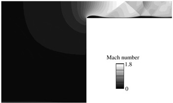
Initial two-dimensional (2D) solutions of the tip flow were found to not become unsteady. Figure 9 shows the predicted Mach number contours for the 2D tip flow. The separation bubble at the inlet to the gap precedes the development of an oblique shock wave which reflects from the casing and goes on to interact with the tip boundary layer, causing a shock-induced separation. The 2D DNS results showed some small-amplitude fluctuations in the flow field, but no unsteadiness was observed in either the primary or the secondary separation (such as vortex shedding within the separated shear layers). Constraining the spanwise extent of the tip flow to
 $0.1g$
could produce a similarly stable result when running 3D simulations, even when the flow was subjected to a forced perturbation.
Example of a simulated flow field; Mach number contours from a solution of the 2D tip flow
 $Re_{g}=15K$
(datum grid).

This implies that the flow is absolutely stable with respect to 2D perturbations and to 3D perturbations with a wavelength smaller than
 $0.1g$
. Although convective instabilities could also cause the flow to become unsteady, in the 2D simulations no perturbations are introduced into the domain and the fact that steady solutions are obtained also in the narrow-domain 3D simulations suggests that the growth rates of the convective instabilities with small spanwise wavenumber are too small to allow for the flow to transition.
The stability of the flow was investigated using a multidimensional linear stability approach in order to determine the spanwise extent required to achieve transition to turbulence within either the primary or the secondary separation bubble. The 2D solutions provided a steady base flow for the stability investigations. The multidimensional stability analysis is conducted by employing DNS with forcing terms, rather than solving a multidimensional eigenvalue problem. Using the converged solutions from 2D DNS as base flow, the forced DNS approach is equivalent to a linear stability analysis on a 2D base flow, and is not restricted to parallel flows. With this approach, the absolute and convective stability characteristics of a given base flow can be investigated similarly to the study by Jones, Sandberg & Sandham (Reference Jones, Sandberg and Sandham2010).
To perform the stability analysis, the 2D results serving as the base flow are read in as the initial condition. In order to maintain the initial condition, or base flow, forcing terms are added to the Navier–Stokes equations
 $$\begin{eqnarray}\frac{\unicode[STIX]{x2202}Q}{\unicode[STIX]{x2202}t}=\text{RHS}-\text{RHS}_{0},\end{eqnarray}$$
where
 $Q$
contains the conservative variables (
 $\unicode[STIX]{x1D70C},\unicode[STIX]{x1D70C}u,\unicode[STIX]{x1D70C}v,\unicode[STIX]{x1D70C}w,\unicode[STIX]{x1D70C}E$
),
 $\text{RHS}$
denotes the right-hand side terms of the Navier–Stokes equations, containing all spatial derivatives, and
 $\text{RHS}_{0}$
are the right-hand side terms of the base flow, i.e. the temporal derivative of the base flow variables
 $(\unicode[STIX]{x2202}Q/\unicode[STIX]{x2202}t|_{t=0})$
.
Thus, at the start of each simulation the right-hand side of the Navier–Stokes equations, containing all spatial derivatives of the basic state, is computed and stored in
 $\text{RHS}_{0}$
. The simulation is then progressed, subtracting the stored forcing term at each Runge–Kutta substep. The result is that, assuming that there is no change or perturbation to the base flow field, the initial condition can be maintained as a reference state, upon which the behaviour of small perturbations can be investigated. This method has been successfully used for stability investigations of aerofoil flows (Jones et al.
Reference Jones, Sandberg and Sandham2010) and supersonic wakes (Sandberg Reference Sandberg2012). It should be noted that this method can only consider discrete modes that depend on the choice of the spanwise domain size and the number of Fourier modes. For that reason, several stability investigations with varying spanwise domain size were conducted for each case and only the simulations exhibiting the largest growth rates are presented in the following.
The centre of the initial pulse added to the higher spanwise Fourier modes was located within the first separation bubble at
 $(x,y)=(0.2,0.03)$
. The perturbation takes the shape of a spatial step function with amplitude
 $1\times 10^{-8}$
with three grid points in the streamwise and wall normal directions. This sharp-edged spatial and temporal distribution will excite a wide range of wavenumbers and frequencies at low amplitude. No further perturbations are introduced, and the response of the flow is monitored as the simulation is progressed. If the flow were convectively unstable, the initial perturbation would be expected to convect downstream while growing in amplitude, ultimately leaving the flow unperturbed. If the flow were absolutely unstable, the initial perturbation would be expected to grow exponentially in time until it reached nonlinear amplitudes, at which point the forced DNS approach loses validity because the force terms will not be able to maintain the base flow. The response of the flow field is monitored by recording the time history of the perturbations at the forcing locations. In the context of a separation region behind a bluff body, it has previously been established that the pulse response, once an initial transient has been overcome, is not sensitive to the location or shape of the pulse, given that the pulse location is within the recirculation region (Sandberg & Fasel Reference Sandberg and Fasel2006).
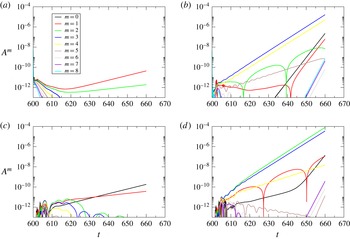
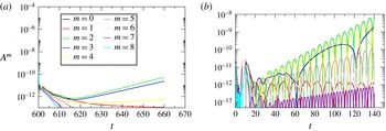
The effect of perturbing the primary separation can be observed in figure 10(a,b). The figure shows the temporal evolution of the amplitudes of eight spanwise Fourier modes within the primary separation bubble when the primary separation experiences a small-amplitude pulse. A domain size of
 $0.8g$
was used, so mode
 $m=1$
corresponds to an instability wave with a spanwise wavelength of
 $0.8g$
. At
 $Re_{g}=1\times 10^{4}$
the flow seems to be marginally unstable for the large-wavelength modes and no growth in the higher modes can be observed, but increasing the Reynolds number to
 $Re_{g}=15\times 10^{3}$
leads to a clear development of an absolute instability. For the case when
 $Re_{g}=15\times 10^{3}$
, modes
 $m=3$
and 4 appear to be the most linearly unstable initially (for the domain size investigated), and these correspond to spanwise wavelengths in the range 0.2–0.27. The other spanwise modes start growing later in time, due to nonlinear interaction between initially linearly unstable modes.
Stability of primary (a,b) and secondary (c,d) separation at
 $Re_{g}=1\times 10^{4}$
(a,c) and
 $Re_{g}=15\times 10^{3}$
(b,d);
 $m=\text{spanwise mode}$
,
 $\text{span}=0.8g$
.

The same procedure was performed perturbing the base flow in the secondary (shock-induced) separation. The stability of the second separation shows a similar behaviour to that of the primary separation (see figure 10
c,d). At
 $Re_{g}=15\times 10^{3}$
, modes
 $m=2$
and 3 appear to be the most unstable initially, providing further confirmation that a spanwise domain size of
 $0.4g$
for the DNS is sufficient.
4.2 Effect of Reynolds number
The preceding section demonstrated the requirement for sufficient spanwise extent in order to allow for inclusion of the unstable spanwise modes that lead to the generation of intermittent 3D structures further downstream. The following results were determined from 3D DNS with a spanwise extent of
 $0.4g$
, which provides sufficient range to capture the most unstable 3D modes (see above). The effect of doubling the span from
 $0.4g$
to
 $0.8g$
was shown previously to have a small influence on the results (see figure 6).
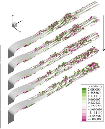
The turbulent structure of the flow can be observed in figure 11. This shows a sequence of instantaneous snapshots of vorticity isosurfaces. The shear layer forming the separation bubble appears to be predominantly laminar, but downstream of the reattachment, hairpin structures appear to develop. The legs of these structures have spanwise spacings of approximately
 $0.15{-}0.2g$
, which agrees well with the previous stability analysis. For the time instants shown here, a patch of turbulent flow is seen propagating downstream, but following and preceding this is a region of relatively steady flow (i.e. possessing hardly any smaller-scale structures).
A sequence of instantaneous snapshots of isosurfaces of vorticity magnitude (
 $\unicode[STIX]{x1D714}=5$
) spaced
 $\unicode[STIX]{x0394}t=0.5$
,
 $Re_{g}=20\times 10^{3}$
(fine grid,
 $\text{span}=0.4g$
, 32 spanwise modes).
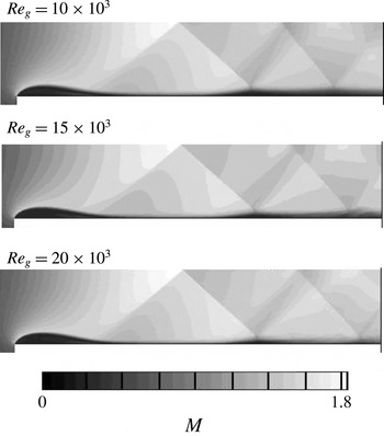
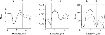
The influence of Reynolds number on the tip flow structure can be observed in figure 12. The most apparent effect of Reynolds number is the change to the secondary separation and shock structure. As the Reynolds number rises, the height of the secondary separation is reduced and the second shock/boundary layer interaction subsequently shifts downstream. The effect of Reynolds number on the surface quantities is shown in figure 13. The influence on the tip surface pressure (identified by the isentropic Mach number) is small in the region of the inlet separation bubble, the reattachment region (marked R) and the supersonic acceleration downstream of the bubble. This suggests that the bubble shape is largely insensitive to Reynolds number, since the shape of the primary separation bubble controls the pressure field in this region. In contrast, near the first shock/boundary layer interaction (marked S), the influence of Reynolds number on the local surface pressure field is significant; as the secondary separation is reduced at higher Reynolds numbers, the free-stream Mach number rises. For boundary layers that are not undergoing transition, the magnitude of the skin friction typically reduces as the Reynolds number is increased. The results upstream of
 $x/g=3$
in figure 13 are consistent with this. Downstream of
 $x/g=3$
, and particularly downstream of the shock/boundary layer interaction (S), the skin friction rises as the Reynolds number is increased. This is because the flow is not fully turbulent, but is in the process of transition, a process that is augmented by increasing the Reynolds number and by the presence of the shock/boundary layer interaction. This has a significant effect on the heat transfer in this region, as also shown in figure 13. The figure shows that upstream of S, the rise in
 $q_{norm}$
is consistent with the rise in Reynolds number (doubling
 $Re_{g}$
leads to approximately an 80 % increase in
 $q_{norm}$
at
 $x/g=2$
). Downstream of S, the effect of doubling the Reynolds number has a proportionately much greater effect; doubling
 $Re_{g}$
leads to a 3.5-fold increase in
 $q_{norm}$
at
 $x/g=4$
.
Spanwise average instantaneous Mach number contours from 3D solutions at various Reynolds numbers;
 $\text{span}=0.4g$
(datum grid, 16 spanwise modes).

Surface isentropic Mach number, skin friction and normalized heat flux on the tip surface for
 $Re_{g}=20\times 10^{3}$
(——),
 $Re_{g}=15\times 10^{3}$
(– – –) and
 $Re_{g}=10\times 10^{3}$
(— ⋅ —);
 $\text{span}=0.4g$
.

4.3 Heat transfer coefficient, adiabatic wall temperature and recovery coefficient
An additional simulation of the
 $Re_{g}=20\times 10^{3}$
case described above was performed at a reduced wall temperature of
 $T_{w}=0.89T_{o}$
, and the difference in wall heat flux between the two cases was used to determine the heat transfer coefficient, adiabatic wall temperature and recovery factor. For convective heat transfer, it is conventionally assumed that the surface heat flux is proportional to a heat transfer coefficient and a driving temperature difference,
 $$\begin{eqnarray}q=h(T_{aw}-T_{w}),\end{eqnarray}$$
where
 $T_{aw}$
is the adiabatic wall temperature (equal to the recovery temperature). Under the assumption that the heat transfer coefficient (
 $h$
) and adiabatic wall temperature are not dependent on
 $T_{w}$
over the range of gas-to-wall temperature ratios tested here (in this case
 $T_{w}/T_{o}$
is changed by 15 %), calculations at two different wall temperatures can be used to determine
 $T_{aw}$
and
 $h$
; (4.2) has two unknowns
 $T_{aw}$
and
 $h$
, and therefore these can be determined using results of the computed surface heat flux at two wall temperatures.
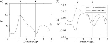
The variation in heat transfer coefficient over the tip surface is shown in figure 14. Also shown are the positions of the primary separation bubble reattachment (R) and the shock/boundary layer interaction (S), as discussed in the previous section. The heat transfer coefficient varies greatly over the tip width, with a minimum value within the primary separation zone of
 $Nu=15$
to a maximum at the reattachment point (R) of
 $Nu=95$
. The effect of the shock/boundary layer interaction at S, which leads to the secondary separation, also causes
 $Nu$
to drop to approximately 15, although the following reattachment point heat transfer coefficient peaks at a lower level of approximately
 $Nu=50$
, as compared with the primary separation point reattachment.
It is interesting to study how the presence of large regions of separated flow and strong free-stream pressure gradients affects the correlation between the skin friction and the heat transfer coefficient. A Reynolds analogy assumption would indicate that the Stanton number (
 $St=h/c_{p}\unicode[STIX]{x1D70C}_{\infty }u_{\infty }$
) and skin friction coefficient are directly proportional to each other, i.e.
 $c_{f}=2St$
. Figure 14 compares
 $c_{f}$
with
 $2St$
over the tip surface. The Reynolds analogy is clearly not adequate over the majority of the tip surface. This departure occurs in regions of separation since, although the skin friction falls to zero, heat transfer will still be possible if there is a driving temperature difference, as shown by Spalart & Coleman (Reference Spalart and Coleman1997) and Spalart & Strelets (Reference Spalart and Strelets2000). This is most pronounced at the reattachment point R, where the skin friction is zero and the heat transfer coefficient is at a maximum. The reattachment point heat transfer is largely driven by turbulence production in this region, and we will discuss this more in the next section. In general, the heat transfer coefficient levels are significantly greater than one would expect from the simple Reynolds analogy. The results show that estimations of tip heat transfer using a Reynolds analogy will significantly underestimate the tip heat load, and this is important from a turbine design perspective.
Variation of the heat transfer coefficient expressed as a Nusselt number (a), and comparison of the Stanton number with the skin friction coefficient (b);
 $Re_{g}=20\times 10^{3}$
,
 $\text{span}=0.4g$
.

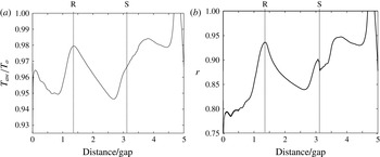
The variation in the adiabatic wall temperature is shown in figure 15. As discussed earlier, data downstream of
 $x/g=4.75$
should be ignored due to the presence of the zonal characteristic condition in this region, and the spike in the adiabatic wall temperature in this region is an artefact of this. Between R and S, the variation in the adiabatic wall temperature is consistent with the distribution of the free-stream Mach number over the tip surface; the lowest value of
 $T_{aw}$
occurs in the region of the peak free-stream Mach number.
The recovery factor (
 $r=(T_{aw}-T_{\infty })/(T_{o}-T_{\infty })$
) is also shown in figure 15;
 $r$
displays quite a considerable variation over the tip from 0.75 to 0.95 between
 $x=0$
and 4.75; low values of
 $r$
occur within the separated regions, and also at the point of peak isentropic Mach number, while peaks in
 $r$
occur within the reattachment zones of both the primary and secondary separation bubbles. Typically, values of the recovery factor of between 0.83 and 0.9 are assumed, depending on the expected boundary layer state and Prandtl number; for 2D self-similar laminar boundary layers the recovery factor can be shown to be approximately equal to
 $Pr^{1/2}$
, and thus for air
 $r\approx 0.85$
(see, for example, Kays & Crawford Reference Kays and Crawford1980). The results shown here are consistent with the range of values of the recovery factor expected for laminar and turbulent boundary layers. There is approximately a 20 % variation in the recovery factor over the tip surface, with higher values of the recovery factor in regions of high turbulent kinetic energy (as shown later in figure 16).
Variation of the adiabatic wall temperature (recovery temperature) (a) and the recovery factor
 $r$
(b);
 $Re_{g}=20\times 10^{3}$
,
 $\text{span}=0.4g$
.

5 Effect of free-stream disturbances, cross-flow and the pressure surface boundary layer on the tip flow
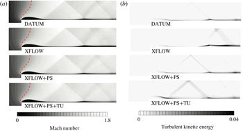
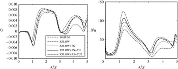
The time-averaged Mach number and the turbulent kinetic energy for the additional DNS performed are shown in figure 16. Comparison of the ‘DATUM’ and ‘XFLOW’ cases shows that the effect of cross-flow appears to have little effect on the size and shape of the primary separation bubble, although the levels of turbulent kinetic energy produced in the primary separation are reduced by approximately 30 % in the reattachment region with the addition of cross-flow. The reason for this is that cross-flow tends to stabilize the tip flow, as will be shown in the stability analysis for the ‘XFLOW’ cases discussed later. The lower levels of turbulence produced in the ‘XFLOW’ case mean that the boundary layer is less able to withstand the downstream shock/boundary layer interaction, and this leads to a much longer region of separated flow downstream of the shock impingement. These effects lead to a significant reduction in both the skin friction and the Nusselt number over the tip surface (see figure 17).
The time-averaged Mach number (a) and the turbulent kinetic energy (b) for the DNS test cases (see table 1); the dashed line indicates the
 $M=1$
contour (
 $Re_{g}=20\times 10^{3}$
,
 $\text{span}=0.4g$
).

The time-averaged skin friction and Nusselt number for the DNS test cases (see table 1).

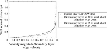
Figure 18 compares the time-averaged boundary layer profile on the pressure side from the XFLOW
 $+$
PS case with the pressure surface boundary layer predicted in the DNS simulations of a transonic high-pressure turbine vane shown in Wheeler et al. (Reference Wheeler, Sandberg, Sandham, Pichler, Michelassi and Laskowski2016). The Reynolds and Mach numbers at the vane exit for this study were
 $0.6\times 10^{6}$
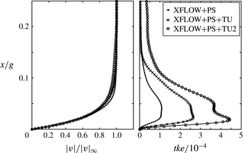
and 0.9 respectively. There is a surprisingly good agreement with the profiles, particularly comparing the vane pressure surface boundary layer profile at 20 % axial chord. Figure 19 compares the pressure side boundary layer profile and turbulent kinetic energy for the cross-flow cases, showing that as the inflow disturbance amplitude is increased there is a significant increase in the turbulence intensity in the boundary layer, but the velocity profile itself does not greatly vary between the cases.
Boundary layer profiles on the pressure side at
 $y=-1.0g$
compared with pressure side boundary layers from HP vane calculations of Wheeler et al. (Reference Wheeler, Sandberg, Sandham, Pichler, Michelassi and Laskowski2016).

Boundary layer profiles on the pressure side at
 $y=-1.0g$
.

The effect of the pressure surface boundary layer can be observed by comparing the ‘XFLOW’ and ‘XFLOW
 $+$
PS’ cases. Figure 17 shows that the presence of the pressure surface boundary layer leads to an increase in the production of turbulent kinetic energy in the primary separation, which consequently raises the skin friction and Nusselt number, and this offsets considerably the opposing stabilizing influence of cross-flow. The reattachment point of the primary separation bubble is not greatly affected by either cross-flow or the pressure surface boundary layer. In contrast, the secondary shock-induced separation is significantly influenced by both cross-flow and the pressure surface boundary layer; the stabilizing effect of cross-flow causes the secondary separation to remain unattached, leading to low skin friction and heat transfer, while the destabilizing effect of the pressure surface boundary layer causes a stronger breakdown to turbulence in the ‘XFLOW
 $+$
PS’ case, which then causes an earlier reattachment of the secondary separation bubble. By comparing ‘XFLOW
 $+$
PS’ with ‘XFLOW
 $+$
PS
 $+$
TU’ and ‘XFLOW
 $+$
PS
 $+$
TU2’ in figure 17, we see that the effect of free-stream disturbances is to raise the skin friction and Nusselt number fairly uniformly over the tip surface. The free-stream disturbances also bring about earlier reattachment of both the primary and secondary separation bubbles.
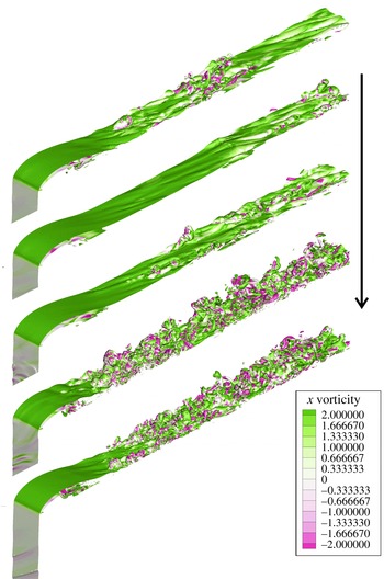
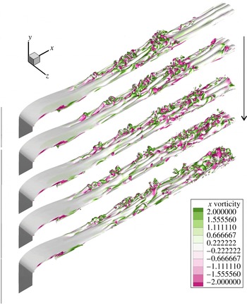
An example of the instantaneous tip gap flow at five sequential time instants is shown in figure 20 for the ‘XFLOW
 $+$
PS
 $+$
TU’ case, and this shows an intermittently turbulent flow field. The turbulent structure of the flow in all cases was observed to be similar to that of the ‘DATUM’ case; the shear layer forming the separation bubble appears to be predominantly laminar, but downstream of the separation, hairpin structures emerge. As in the ‘DATUM’ case, the legs of these structures have a spacing of approximately
 $0.15{-}0.2g$
. In the penultimate image, there also appear to be structures propagating up the pressure surface and into the tip gap, affecting the separation bubble and bringing about a rapid breakdown to turbulence directly.
Instantaneous snapshots showing isosurfaces of vorticity magnitude (
 $\unicode[STIX]{x1D714}=5$
) for the ‘XFLOW
 $+$
PS
 $+$
TU’ case; time between snapshots
 $\unicode[STIX]{x0394}t=9.6$
.

5.1 Stability analysis with cross-flow
We reported on the stability of the ‘DATUM’ case above and showed that breakdown to turbulence came about due to an absolute instability of the primary separation bubble. A stability analysis for the cross-flow cases (‘XFLOW’ and ‘XFLOW
 $+$
PS’) is now discussed. As described above, the multidimensional stability analysis is conducted by employing DNS with forcing terms, rather than by solving a multidimensional eigenvalue problem.
The effect of perturbing the primary separations in the ‘XFLOW’ and ‘XFLOW
 $+$
PS’ cases can be observed in figure 21. This figure shows the temporal evolution of the amplitudes of eight spanwise Fourier modes within the primary separation bubble when the primary separation experiences a small-amplitude pulse. For both cases, a domain size of
 $1.5g$
was used. It can be observed that the most unstable mode for the spanwise domain size investigated is
 $m=2$
in both cases, which corresponds to an instability wave with spanwise wavelength of
 $0.75g$
. As also observed in the ‘DATUM’ case, the separation is absolutely unstable; however, the instability growth rates are reminiscent of those found at
 $Re_{g}=1\times 10^{4}$
without cross-flow. In the original analysis for the ‘DATUM’ case, it was found that the growth rates were reduced at lower Reynolds numbers, and thus the effect of cross-flow is similar to reducing the tip Reynolds number. The introduction of cross-flow also leads to a shift to lower instability modes and thus larger wavelengths from
 $0.25g$
(‘DATUM’) to
 $0.75g$
for both cross-flow cases shown here. Earlier stability analyses by Sandberg (Reference Sandberg2012) showed that a shift to lower instability modes can occur when including eddy viscosity in the stability analysis, which in essence also reduces the effective Reynolds number. Previous work on separation in cross-flow on swept aerofoils (such as Horton Reference Horton1968) has suggested that the stability of the separation can be determined from the Reynolds number resolved in the chord-wise direction (i.e. the direction orthogonal to the leading edge). This theory of independence of the chord-wise and cross-flow boundary layers (Horton Reference Horton1968) would suggest that for the same streamwise Reynolds number, the addition of cross-flow would reduce the chord-wise Reynolds number and thus we would expect an increased region of laminar flow with cross-flow. For our case, the Reynolds number based on the
 $u$
component of velocity is approximately 4 % lower than the streamwise Reynolds number (see § 2), and is unlikely to explain fully the increased stability of the cross-flow cases.
Growth of instability waves for (a) the ‘XFLOW’ case and (b) the ‘XFLOW
 $+$
PS’ case. (Spanwise extent
 $=1.5g$
.)

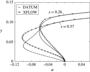
Another explanation is that the addition of cross-flow reduces the magnitude of the reverse flow within the separation bubble, and evidence for this is seen in the skin friction data shown in figure 17. This is also seen in figure 22, which shows the variation of the
 $x$
component of velocity at two positions in the separation bubble (
 $x=0.26g$
and
 $x=0.57g$
) for the ‘DATUM’ and ‘XFLOW’ cases; the profiles show that the effect of cross-flow is to reduce the magnitude of the reverse flow in the near-wall region (
 $y<0.04g$
).
An additional DNS cross-flow case was performed to determine whether the spanwise extent of
 $0.4g$
was sufficient for the cross-flow cases, given the shift to lower instability modes observed in the stability analysis discussed above. Figure 23 shows the predicted skin friction for the ‘XFLOW’ case with spanwise extents of 0.4 and
 $0.8g$
; the spanwise resolution was kept constant by doubling the number of spanwise modes for the case with
 $0.8g$
spanwise extent. The skin friction in the region of reattachment downstream of the secondary separation is modified by the increased spanwise extent. Nonetheless, there is little difference in the skin friction in the region of the primary separation bubble and first reattachment point, as well as the position of the secondary separation, indicating that even for the cross-flow cases, a spanwise extent of
 $0.4g$
is sufficient for capturing the correct boundary layer state over the majority of the tip width.
Profile of reversed flow in the separation bubble for the ‘DATUM’ and ‘XFLOW’ cases at
 $x=0.26g$
and
 $x=0.57g$
.

Skin friction predictions for the ‘XFLOW’ case with different spanwise extents.

6 Conclusion
Direct numerical simulations were conducted to investigate the unsteady flow over a model turbine blade tip at engine-scale Reynolds and Mach numbers. The particular case of a transonic tip flow was studied since previous work had suggested that compressibility has an important influence on the turbulent nature of the separation bubble at the inlet to the gap and subsequent flow reattachment. The flow was simulated over an idealized tip geometry where the tip gap was represented by a constant-area channel with a sharp inlet corner to represent the pressure side edge of the turbine blade. We investigated the influence of free-stream disturbances, cross-flow and the pressure side boundary layer on the tip flow aerodynamics and heat transfer. For ‘clean’ inflow cases we found that even at engine-scale Reynolds numbers the tip flow is intermittent in nature (neither steady nor fully turbulent). The breakdown to turbulence occurs through the development of spanwise streaks with a spacing of approximately 15 %–20 % of the gap height. Linear stability analysis of steady 2D Navier–Stokes solutions of the same set-up found the most unstable global modes to have spanwise wavelengths of approximately 25 % of the gap height. Cross-flows of 25 % of the gap exit velocity were found to increase the stability of the tip flow, and to significantly reduce the turbulence production in the separation bubble. This was also predicted through the linear stability analysis. For the case when the inlet flow contained free-stream disturbances, viscous dissipation and the rapid acceleration of the flow at the inlet to the tip gap caused significant distortion of the vorticity field and reduction of turbulence intensity as the flow entered the tip gap. It was also shown that the Reynolds analogy generally does not hold, in particular in regions where the skin friction approaches zero while a significant temperature gradient is present, such as at the reattachment point of the tip flow. Furthermore, the DNS results indicate up to 20 % variation in the recovery factor over the tip surface, suggesting that the common assumption of constant recovery factor is inaccurate.
Acknowledgements
Computer time was provided by the UK turbulence consortium under EPSRC grant EP/L000261/1. This work was also supported by resources provided by The Pawsey Supercomputing Centre with funding from the Australian Government and the Government of Western Australia.