





1. Introduction
Social preferences have been shown to play an important role in a wide variety of domains such as the labor market (e.g., Bellemare & Shearer, Reference Bellemare and Shearer2007; Charness, Reference Charness2000; Dur, Reference Dur2009; Fehr et al., Reference Fehr, Kirchsteiger and Riedl1993; Kube et al., Reference Kube, Maréchal and Puppe2012), bargaining decisions (e.g., Camerer, Reference Camerer2011; Camerer & Loewenstein, Reference Camerer and Loewenstein1993; Camerer & Thaler, Reference Camerer and Thaler1995), political economy (e.g., Fehr ⓡ al., Reference Fehr, Epper and Senn2024; Fisman et al., Reference Fisman, Jakiela and Kariv2017; Henkel ⓡ al., Reference Henkel, Fehr, Senn and Epper2025; Kerschbamer & Müller, Reference Kerschbamer and Müller2020; Tyran & Sausgruber, Reference Tyran and Sausgruber2006), and contract design (e.g., Bierbrauer & Netzer, Reference Bierbrauer and Netzer2016; Bierbrauer et al., Reference Bierbrauer, Ockenfels, Pollak and Rückert2017; Fehr et al., Reference Fehr, Powell and Wilkening2021; Schmidt & Ockenfels, Reference Schmidt and Ockenfels2021), among others. Given their theoretical and empirical relevance, it is critical to measure them accurately. In this context, a particularly important question is whether monetary incentives matter for the elicitation of social preferences.Footnote 1
In contrast to other disciplines, the use of monetary incentives has been a pillar of experimental economics (Hertwig & Ortmann, Reference Hertwig and Ortmann2001; Plott, Reference Plott1986; Smith, Reference Smith1982, Reference Smith1991). Among others, behaviors measured using incentivized decisions are believed to more accurately capture subjects’ “true preferences” than self-reported answers in hypothetical scenarios. In the context of social preferences, where concerns regarding social desirability are particularly high, there are good reasons to believe that monetary incentives might matter for the weight that people put on others’ payoffs.Footnote 2 However, incentivizing decisions also comes at a cost for researchers, who often need to spend thousands of dollars to incentivize the decisions of their participants. This raises the following question: Do monetary incentives improve the measurement of social preferences, or can a non-incentivized elicitation method mimic the properties of an incentivized task?
We study this question using a pre-registered online experiment conducted on Prolific with over 3,000 subjects broadly representative of the US population.Footnote 3 Broad population samples have, for example, been used to study questions such as the role of social preferences for political support for redistribution (Fehr ⓡ al., Reference Fehr, Epper and Senn2024; Fisman et al., Reference Fisman, Jakiela and Kariv2017; Henkel ⓡ al., Reference Henkel, Fehr, Senn and Epper2025; Kerschbamer & Müller, Reference Kerschbamer and Müller2020), to get a deeper understanding about how people reason about the economy (Andre et al., Reference Andre, Pizzinelli, Roth and Wohlfart2022; Stantcheva, Reference Stantcheva2021), or to study the role of beliefs for willingness to act against climate change (Dechezleprêtre et al., Reference Dechezleprêtre, Fabre, Kruse, Planterose, Chico and Stantcheva2025; Falk et al., Reference Falk, Andre, Boneva and Chopra2021), among others. The question of the role of monetary incentives for the identification of social preferences in broad population samples is particularly relevant given that several survey providers do not allow to incentivize decisions. In this context, understanding whether incentivization matters is an important empirical question.
We elicit social preferences using a set of choice situations in which the decision-maker has to decide on how to allocate resources, which are provided by the experimenter, between herself and an anonymous other participant (Fehr ⓡ al., Reference Fehr, Epper and Senn2024).Footnote 4 While the literature has often relied on simple dictator games (i.e., choice situations in which subjects can sacrifice resources to increase the payoff of others) to identify social preferences, our experimental paradigm also includes several decision situations where the decision-maker can pay in order to decrease the payoff of others. This allows for the identification of a broader range of social preferences. Indeed, while standard dictator games are well suited to identify altruism and the extent to which individuals are willing to trade-off equality and efficiency (see, e.g., Fisman et al., Reference Fisman, Kariv and Markovits2007, Reference Fisman, Jakiela and Kariv2017), they do not allow to identify a broad range of other social preferences. For example, inequality aversion (Bolton & Ockenfels, Reference Bolton and Ockenfels2000; Charness & Rabin, Reference Charness and Rabin2002; Fehr & Schmidt, Reference Fehr and Schmidt1999) implies that individuals might not only be willing to sacrifice some of their own payoff to increase the payoff of those worse off (aversion to advantageous inequality), but also to decrease the payoff of those who are better off (aversion to disadvantageous inequality). Similarly, envious and spiteful individuals are willing to pay to destroy the payoff of others. Our design solves this identification issue.
To identify the effects of monetary incentives, we exogenously vary whether decisions are incentivized, and by how much. In the Low- and the High-Incentives treatments, decision-makers are paid on the basis of their choice in a randomly drawn choice situation. These two treatments, in which stakes are scaled by a factor of 5, allow us to assess whether the strength of monetary incentives matters for the identification of social preferences.Footnote 5 In the Hypothetical treatment, subjects’ decisions were not incentivized, but decision-makers were encouraged to make a decision “as if” decisions were incentivized. Together, these treatments allow us to cleanly identify whether and how monetary incentives affect the identification of social preferences. We explore these questions in several steps.
First, we investigate whether and how monetary incentives affect subjects’ modal choices at the descriptive level. Specifically, we examine the effects of monetary incentives for subjects’ willingness to pay to increase the other participants’ payoff (modal choice on negatively sloped budget lines), and for their willingness to pay to decrease the other participants’ payoff (modal choice on positively sloped budget lines). In all treatments, we find that subjects’ choices are strikingly similar, irrespective of whether decisions are incentivized or not, and irrespective of the size of the monetary stakes.
Second, we assess whether monetary incentives play a role in the distribution of social preference types in the population. To answer this question, we uncover the distribution of preferences in each treatment by applying the Dirichlet Process means (DP-means) algorithm, a Bayesian nonparametric clustering algorithm. In all the treatments, we find that the same three clusters with a clear behavioral interpretation emerge: an inequality-averse type, an altruistic type, and a predominantly selfish type. Moreover, the distribution of types is remarkably similar across treatments, with each type comprising about one third of subjects in all treatments. These findings are noteworthy, given that the DP-means algorithm does not impose any assumptions on the behavioral interpretation of types nor on their distribution.
Third, we assess whether monetary incentives affect the strength of social preferences. To answer this question, we compare across the different treatments the (distributions of) structurally estimated parameters of a model of social preferences that comprises inequality aversion, altruism, and envy as special cases (Charness & Rabin, Reference Charness and Rabin2002; Fehr & Schmidt, Reference Fehr and Schmidt1999). In all treatments, the average estimated levels of other-regardingness are sizeable. Indeed, our structural estimates of aversion to disadvantageous inequality (the  $\alpha$-parameter in the Fehr-Schmidt model) range from 0.219 in the Low-Incentives to 0.368 in the Hypothetical treatments, corresponding to a willingness to pay of 18–26.9 cents to decrease the payoff of those ahead by one dollar. Turning to aversion to advantageous inequality (the
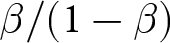
 $\beta$-parameter in the Fehr-Schmidt model), we estimate parameters ranging from 0.613 in the Low-Incentives to 0.744 in the Hypothetical treatment, corresponding to a willingness to pay to increase the payoff of those worse off by one dollar of 1.58 and 2.90, respectively. Importantly, we find that the size of the monetary stakes (Low- vs. High-Incentives) does not play a large role in the strength of social preferences. However, social preference parameters are consistently larger – i.e., likely to be overestimated – when stakes are hypothetical. Interestingly, we show that these treatment differences are mainly driven by subjects identified as being inequality averse by the clustering algorithm. For these subjects, a lack of monetary incentives yields a larger aversion to both advantageous and disadvantageous inequality.
We also explore how monetary incentives affect the precision of structural estimates. To that end, we compare individuals’ posterior standard deviation of the estimated social preference parameters.Footnote 6 We find that the precision of the estimates improves substantially when moving from the hypothetical to the incentivized treatments, suggesting that preference parameters recovered under monetary incentives are more reliable and better measures of social preferences. The precision of estimated preference parameters in the low and the high incentives treatment is, however, quite similar.
Together, our results indicate that monetary incentives and stake size have only small effects on subjects’ modal choices and on the identification of qualitatively distinct preference types. However, they do affect the quantitative assessment of the strength and precision of social preferences. In particular, our structural analysis suggests that social preferences tend to be overestimated when elicited using hypothetical stakes. These findings imply that whether or not one should use incentives to elicit social preferences depends on the research objective. If one is interested in obtaining a rough, aggregate measure of social preferences (e.g., in terms of subjects’ modal choices) or in identifying qualitatively distinct preference types, then hypothetical stakes may suffice. If, however, one is interested in quantitative estimates, e.g., to quantitatively calibrate a theoretical model that is then used for predictive purposes, then the use of monetary incentives is advisable, as hypothetical stakes appear to inflate inequality aversion and lead to much more imprecisely estimated preference parameters.
While our paper and the results above are based on a large sample drawn from the general population, it is also interesting to understand the role of monetary incentives for the identification of social preferences in students. Indeed, student samples are still widely used in economic experiments, and insights from the general population might not extend to students. To shed light on this issue, we also collected an additional sample of students carefully prescreened from Prolific.Footnote 7 In a nutshell, we find that some of our conclusions extend to students: the use of monetary incentives (and their size) appears to have little effect on the identification of social preferences, both at the descriptive level of subjects’ modal choices and in the clustering analysis. The results of the structural analysis are a little less clear-cut, as we find the largest levels of inequality aversion (and the lowest precision in the estimates) in the High-Incentives treatment. However, these results need to be interpreted with caution because our student sample is much less well-powered than our general population sample.
Our paper is connected to the literature interested in the effects of using monetary incentives in experimental research. In particular, our paper is linked to studies that have investigated the effects of monetary rewards for behavior in dictator games using student samples.Footnote 8 An early contribution to this literature is Forsythe et al. (Reference Forsythe, Horowitz, Savin and Sefton1994), who compare the effects of incentivized versus hypothetical decisions in a dictator game. They find that dictators donate significantly less when decisions are incentivized. They also study the effects of stake sizes ($5 vs $10) and cannot reject the hypothesis that stakes do not affect behavior.Footnote 9 More recently, Bühren & Kundt (Reference Bühren and Kundt2015) report on an experiment where participants are asked to make decisions in three games (a prosocial, an envy, and a sharing game). Subjects are randomized into a treatment condition where decisions are incentivized or a condition where decisions are hypothetical. They find that participants in the incentives treatment display more spite and less inequality aversion. Clot et al. (Reference Clot, Grolleau and Ibanez2018) compare the effects of different compensation mechanisms in a dictator game and find that hypothetical stakes lead to fewer egoistic and more egalitarian decisions.Footnote 10
Engel (Reference Engel2011) reviews the literature on dictator games in his meta-analysis, covering over 100 papers published prior to 2010. On the role of incentives, he concludes that dictators’ behavior when decisions are incentivized is not significantly different than when their decisions are hypothetical. He only finds very weak evidence that stake size affects giving, despite covering studies with dramatic changes in stake sizes ranging from $0 to $130.Footnote 11 These results are largely confirmed by a more recent meta-analysis by Larney et al. (Reference Larney, Rotella and Barclay2019), who find a significant but small effect of stake size on dictator game offers (and no effect of stakes on ultimatum game offers). Note, however, that this meta-analysis excluded studies with hypothetical stakes, and therefore cannot provide evidence on the effects of incentivization per se.
More recently, Hufe & Weishaar (Reference Hufe and Weishaar2025) studied the effects of incentives for fairness ideals. They find that respondents make similar choices when allocating monthly earnings between two persons in a spectator design, independent of whether decisions are hypothetical or not.Footnote 12 Kosfeld et al. (Reference Kosfeld, Sharafi, Sontag González and Zou2025) conducted a cross-cultural validation of the (Global) Preference Survey Module (Falk et al., Reference Falk, Becker, Dohmen, Enke, Huffman and Sunde2018, Reference Falk, Becker, Dohmen, Huffman and Sunde2023) and found that quantitative survey items (hypothetical experiments) aimed at capturing social preferences tend to be good predictors of behavior in related incentivized choice experiments.Footnote 13 Last, Fitzgerald (Reference Fitzgerald2024) shows that traditional hypothetical bias measures are often misleading estimates of hypothetical bias for intervention experiments.
Our results contribute to the existing literature in several ways.
First, our study goes beyond comparing choices in dictator games or ultimatum games across incentive conditions. Instead, we study whether incentives matter (i) for subjects’ willingness to pay to increase the payoff of others, and for their willingness to decrease the payoff of others, (ii) for the distribution of social preference types, where we uncover social preferences using state-of-the-art Bayesian nonparametric methods, and (iii) for the strength of social preferences and the precision of their structural estimates. As such, the scope of this study is – to the best of our knowledge – much broader than the existing studies on the role of monetary incentives for social preferences.
Second, while previous research has investigated the effects of monetary incentives for behavior in dictator games, these studies often rely on student samples of relatively modest size. In contrast, our study addresses this question in a much larger sample drawn from the general population. In our view, this is important given that such samples are being increasingly used by researchers as they are economically much more relevant than student samples.
Finally, the fact that this paper reports on an ex-ante carefully pre-registered experiment and analysis lends further credibility to the empirical findings we document. In this sense, this study also contributes to the broader discussion on best practices in scientific research and the role that pre-registered studies and registered reports can play at increasing transparency in science (Miguel, Reference Miguel2021; Munafò et al., Reference Munafò, Nosek and Bishop2017; Nosek et al., Reference Nosek, Ebersole, DeHaven and Mellor2018).
2. Experimental design
2.1. Measuring distributional preferences
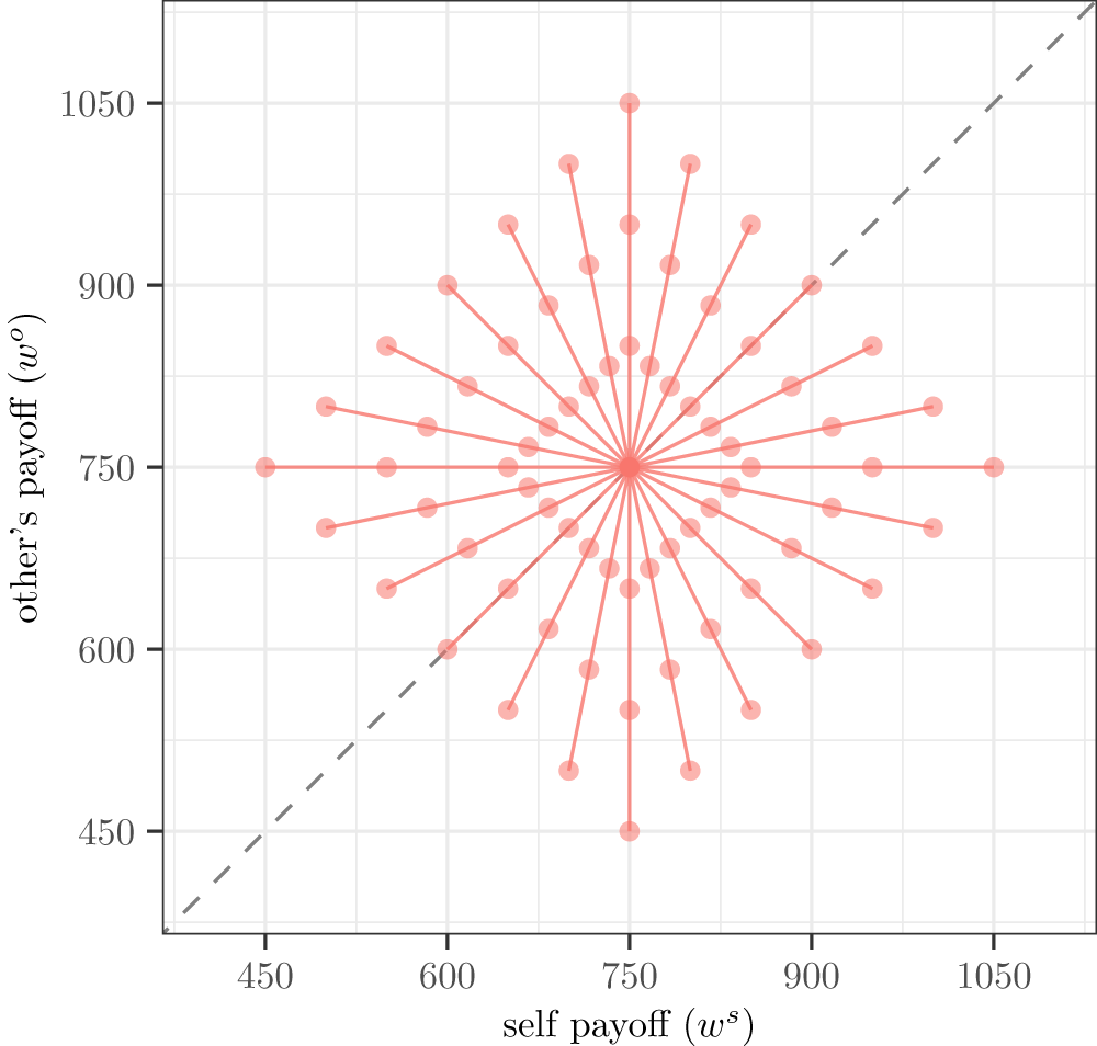
We elicited respondents’ distributional preferences using a series of 12 incentivized money allocation tasks in which participants had to decide how to allocate experimental currency units (ECUs) between themselves and an anonymous other participant of the study. Figure 1 depicts these 12 budget lines, where the decision-maker’s own payoff is represented on the  $x$-axis and the recipient’s payoff is on the
 $y$-axis.Footnote 14
Budget lines used to identify other-regarding preferences

These 12 choice situations systematically vary the cost and the efficiency consequences of redistribution, thereby allowing us to identify a wide range of other-regarding behaviors. Negatively sloped budget lines (where subjects can sacrifice resources to increase the payoff of the other participant) allow us to identify behaviors such as altruism and aversion to advantageous inequality. Positively sloped budget lines (where subjects can pay to decrease the payoff of the other) allow us to identify behaviors such as envy, spite, and aversion to disadvantageous inequality, among others.
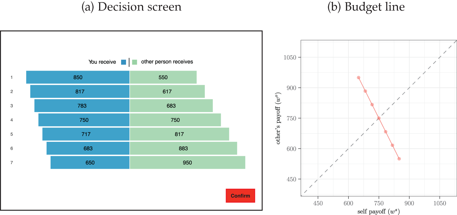
Choice situations were presented to subjects in random order directly on the subjects’ screens. They were presented in a way that made the distributional consequences of each allocation transparent. Figure 2(a) illustrates how a typical choice situation was presented to our participants. In each choice situation, subjects were able to choose between seven interpersonal allocations (labeled by 1–7) – all of them located on a budget line. Each available allocation consisted of a specific distribution of ECUs between the participant (bars labeled by “You receive”) and the other person (bars labeled by “other person receives”). We represented the available choices numerically and graphically in order to make the trade-offs and the associated payoff implications salient. Figure 2(b) plots the budget line corresponding to the example depicted in Figure 2(a) in the ( $\omega^s$,
 $\omega^o$)-space (“own payoff,” “other’s payoff”). In this example, the slope of the budget line is
 $-$2, indicating that for every ECU the decision-maker gives up, the other player receives two ECUs. Here, perfect equality in payoffs can be achieved by choosing allocation 4.
Example choice situation: (a) decision screen and (b) budget line

Fig. 2 Long description
Image A shows a horizontal stacked bar chart with two series labeled You receive and other person receives. Seven rows are labeled 1 through 7. The values shown inside the bars are: 1: 850 and 550. 2: 817 and 617. 3: 783 and 683. 4: 750 and 750. 5: 717 and 817. 6: 683 and 883. 7: 650 and 950. A button labeled Confirm appears at the lower right. mage B shows a budget line with seven possible allocations, and the 45° line.. The horizontal axis label is self payoff (omega superscript s). The vertical axis label is other’s payoff (omega superscript o). The horizontal axis shows tick labels 450, 600, 750, 900, 1050. The vertical axis shows tick labels 450, 600, 750, 900, 1050. The connected points lie on a downward sloping line, including a point at the intersection of the 45° line near 750 on the horizontal axis and 750 on the vertical axis.
2.2. Treatments
To assess the effects of monetary incentives on measures of social preferences, we randomized individuals into one of the following three treatments in a between-subjects design.
Low-Incentives. In this treatment, the decisions of participants had real monetary consequences for them and for another, anonymous participant of the study.Footnote 15 The exchange rate between points and USD was set to 500 points = USD 1.
High-Incentives. In this treatment, the stake size was substantially larger than in the Low-Incentives treatment, as we set the exchange rate to 100 points = USD 1, i.e., stakes were five times larger than in the Low-Incentives treatment.
Hypothetical. In this treatment, participants’ choices were hypothetical. Thus, their decisions neither affected their own payoff nor the payoff of another participant. However, our instructions invited subjects to make decisions as if they were incentivized.
Importantly, we made the consequences of subjects’ decisions salient by highlighting them in the relevant parts of the instructions (bold fonts). In addition, we included a control question specifically aimed at ensuring that participants understood whether their decisions had real monetary consequences or not (see the control questions at the end of the instructions in Appendix A.2). This was crucial to prevent confusion about the nature of the task, especially in the Hypothetical treatment where incentives were absent. By drawing attention to the presence or absence of incentives and verifying comprehension, we aimed to minimize noise in the measurement of social preferences stemming from misunderstandings. This, in turn, increases our confidence that any observed differences in behavior across treatments are attributable to the incentive structure, rather than differences in understanding.
2.3. Sample
We conducted our study with a general population sample that is broadly representative of the US population with respect to age, gender, and political affiliation. Our final sample comprises 3,032 subjects, recruited on Prolific.Footnote 16 Descriptive statistics on participants’ main socio-demographic characteristics can be found in Table B.1 in Appendix B. The average respondent in our sample is 46.2 years old and the share of men is 48.3%. In terms of political leaning, 33.3% of our sample leans towards the Republican Party, while 40.8% leans towards the Democratic Party. The remaining 25.9% lean towards the Independent or no party. In addition, the last column of Table B.1 also shows that the treatments are generally well balanced among the main observable characteristics.
While our main analysis relies on the general population sample, it is also interesting to understand the role of monetary incentives for the identification of social preferences in students. To shed light on this issue, we collected responses from an additional 320 students carefully prescreened from Prolific.Footnote 17 The advantage of recruiting students directly from Prolific is that it keeps the entire experimental protocol constant, thereby enhancing the comparability between the results from the general population and the results from the student sample. For the analysis, we pool the 320 subjects recruited in this separate student sample with the 175 students contained in the general population sample, which were identified using the same screening-criteria. Results for this student sample are reported in Appendix F.
2.4. Data collection and experimental protocol
The experiment was fully computerized using Qualtrics and all the instructions were displayed directly on participants’ screens. The study included control questions for the money allocation task. These questions aimed at identifying participants who did not understand the task or did not pay attention (Berinsky et al., Reference Berinsky, Margolis and Sances2014). Participants who failed to pass these control questions were excluded from the final sample. We provide a transcript of the instructions and control questions displayed on participants’ screens in Appendix A.2.
All participants were paid a show-up fee of USD 3, provided that they completed the study until the end. In addition, we incentivized respondents’ choices in the Low-Incentives and the High-Incentives treatment by implementing one of their decisions at random.Footnote 18
We pre-registered the study on the AEA RCT registry (AEARCTR-0015147), where we uploaded the (accepted) Stage 1 version of this registered report, along with a detailed pre-analysis plan.Footnote 19 Ethics approval was obtained from the Human Subjects Committee of the Department of Economics of the University of Zurich (OEC IRB #2024-043).
3. Hypotheses
Our experimental design allows us to shed light on the effects of monetary incentives on measures of social preferences. A key feature of our study is that we investigate this question at different levels of analysis. In particular, we examine the distribution of qualitatively distinct preference types in a population (clustering analysis), and we assess both the strength and the precision of these preferences (structural analysis). Thus, our hypotheses consider both of these dimensions.Footnote 20
Our first hypothesis relates to whether relying on incentivized decisions is critical for the measurement of social preferences, or whether hypothetical questions suffice. In the context of social preferences, where concerns regarding social desirability are particularly relevant, individuals might not reveal their true preferences in the absence of real monetary stakes. For example, it is costless for a subject to behave in an altruistic way if decisions are hypothetical. If that is the case, hypothetical stakes might lead to an overestimation of the extent to which individuals are other-regarding. This can be particularly problematic if quantitative estimates are used to make behavioral predictions. Tying subjects’ payment to their decisions might mitigate this issue by forcing decision-makers to more carefully trade off their own material benefit with other-regarding concerns.
Hypothesis 1. Monetary incentives do not affect measures of social preferences.
If our results show that monetary incentives do not affect measures of social preferences, researchers could more broadly adopt our elicitation procedure with hypothetical stakes. This would be particularly appealing in contexts where incentivization is logistically difficult to organize (e.g., some online studies) or very costly. If, in contrast, our results show that monetary incentives do affect social preferences, then we will be able to assess how large the mismeasurement related to hypothetical stakes is. This could be particularly useful for researchers who cannot incentivize their subjects but want to know how large the bias due to lack of incentives is likely to be.
Our second hypothesis relates to the effects of stake size. While the social preferences elicited under hypothetical stakes might differ from those elicited with real monetary stakes (Hypothesis 1), it is also possible that the size of the monetary stakes matters for the measurement of social preferences. In particular, larger stakes might affect the distribution of social preferences in a population. This might be the case if, for example, larger stakes induce decision-makers to make more selfish decisions. It is also possible that higher stakes increase the precision with which social preferences are estimated, e.g., if higher stakes lead participants to think more carefully about their decisions.
Hypothesis 2. The strength of monetary incentives has no effect on measures of social preferences.
If our results suggest that the stake size does not matter, then researchers could largely rely on low-powered incentives to reliably elicit social preferences. It is, however, also possible that stake size will affect social preferences. In particular, as discussed above, stakes might affect the precision with which social preferences are estimated. If this is the case, then researchers interested in precisely estimating the strength of social preferences may want to rely on using high-powered incentives to elicit preferences, whereas researchers only interested in the qualitative nature of preferences may rely on low-powered incentives.
Finally, it is important to note that answers to the two hypotheses above might vary depending on whether one considers results from the clustering analysis or the structural analysis. For example, it is possible that there are no treatment differences in all the dimensions in which we assess social preferences, e.g., that the same behavioral types emerge in the same proportions across treatments and that the structurally estimated parameters are identical. However, it is also possible that treatment differences exist in only some dimensions. For example, it is plausible that the distribution of preference types as identified by the clustering remains stable across treatments, but that there are treatment differences in the structurally estimated parameters. Such a result would imply that the nature of the research questions should determine whether monetary incentives should be used or not: Researchers only interested in assessing the qualitative nature of behavioral types and their prevalence in the population could rely on either hypothetical or real monetary stakes, while researchers interested in the quantitative distribution of types and the strength of these preferences should carefully consider using the appropriate incentivization method.
4. Results
This section closely follows the analysis plan that we pre-registered. In some instances, we also provide additional analyses that were not pre-registered but that are useful to further clarify our findings. For transparency, we list these additional analyses in Appendix D.1.
4.1. Descriptive analysis
We start our analysis by exploring subjects’ choices at the descriptive level. For each budget line, we label the own-payoff maximizing allocation by  $z = 1$, the own-payoff-minimizing allocation by
 $z = 0$, and the payoff-equalizing allocation by
 $z = 0.5$. The other four available allocations on each budget line are equidistantly placed between 0–0.5 and 0.5–1, respectively. We are interested in the following questions:
• How do incentives affect subjects’ choices in the money allocation task at the descriptive level?
• Do incentives affect subjects’ willingness to pay to decrease the other participant’s payoff?
• Do incentives affect subjects’ willingness to pay to increase the other participant’s payoff?
To answer these questions, we examine whether the treatments affect the distribution of subjects’ modal choice separately for negatively sloped and for positively sloped budget lines (Figure 1). The distinction between negatively and positively sloped budget lines is important because behavior across budget lines within the class of negatively sloped budget lines informs us about how much money individuals are willing to sacrifice to increase another individual’s payoff, whereas behavior across budget lines within the class of positively sloped budget lines informs us about how much money individuals are willing to sacrifice to decrease another individuals’ payoff. We focus on the mode because it is less susceptible to random responses and to outliers than the mean or the median.Footnote 21
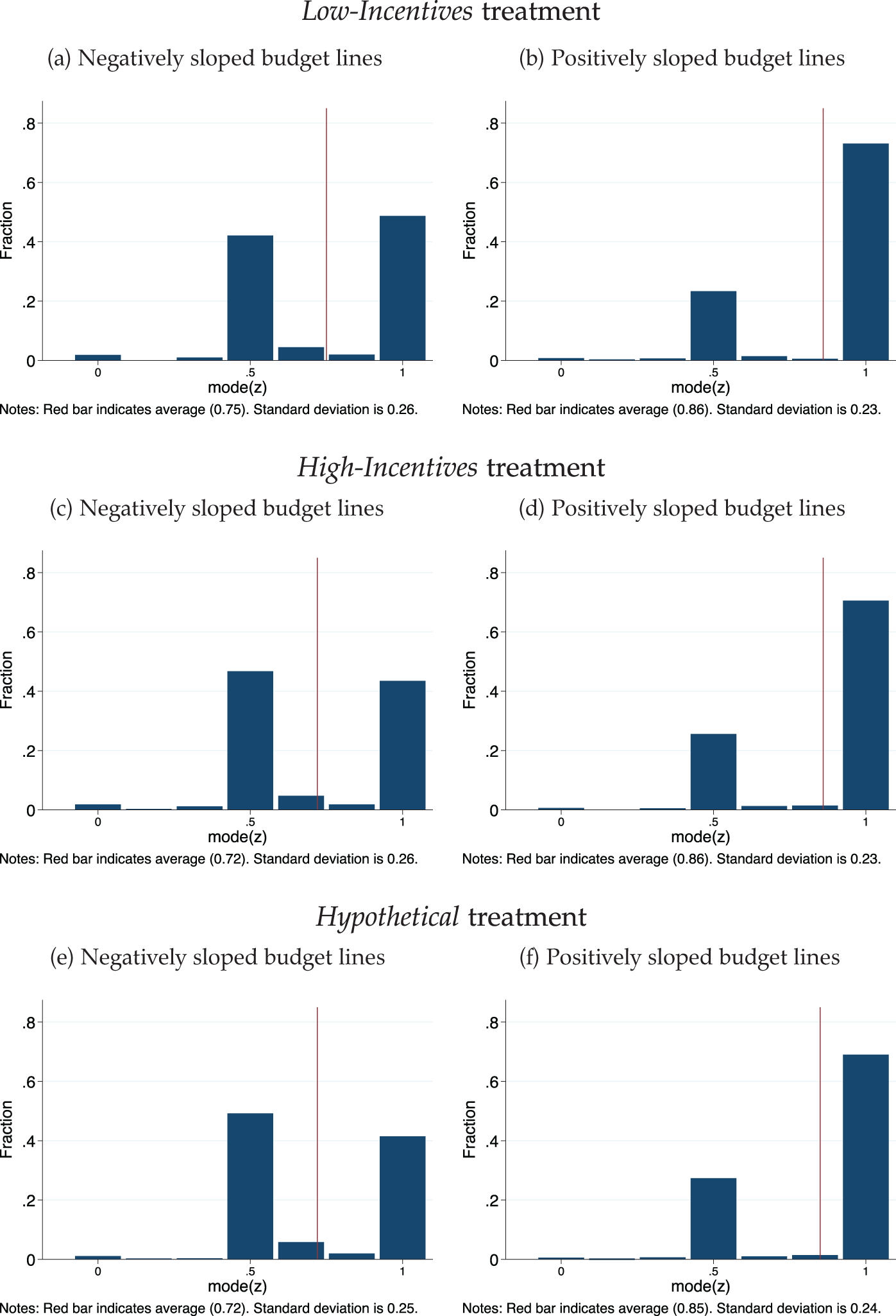
We depict the results of this analysis in Figure 3. The figure reveals that the distributions of modal choices are strikingly similar across treatments. Among the negatively sloped budget lines, the modal choice of the vast majority of individuals is located at either  $z = 0.5$ or
 $z = 1$. For example, in the Low-Incentives treatment, the modal choice of 42.12% of the participants is
 $z = 0.5$, whereas it is
 $z = 1$ for 48.70% of the participants. This means that the majority of participants predominantly choose either the allocation that perfectly equalizes their and the other person’s payoff (
 $z=0.5$), or the one that maximizes their own payoff (
 $z=1$). Likewise, in the High-Incentives treatment, the modal choice of 46.72% of the participants is to equalize payoffs (
 $z = 0.5$), while it is to maximize own payoffs (
 $z = 1$) for 43.50% of the participants in this treatment. These shares are remarkably similar to the ones observed in the Hypothetical treatment, where the modal choice is
 $z = 0.5$ for 49.19% of the participants, and
 $z = 1$ for 41.46%.
Turning to behavior on positively sloped budget lines, own payoff maximization ( $z=1$) is the modal choice of the majority of individuals, while the share of people predominantly implementing payoff equality (
 $z = 0.5$) is much smaller. For example, in the Low-Incentives treatment, 73.14% of the participants predominantly choose the allocation that is own-payoff maximizing (
 $z = 1$), while only 23.30% predominantly pick the payoff-equalizing allocation. The distribution of modal choices in the High-Incentives treatment is very similar: 70.56% predominantly pick the own-payoff maximizing allocation, while only 25.57% predominantly pick
 $z=0.5$. Likewise, in the Hypothetical treatment, we find that 69.01% mainly choose the own-payoff maximizing allocation, and 27.32% the payoff-equalizing allocation.Footnote 22
These first results suggest that monetary incentives do not affect subjects’ willingness to pay to increase and decrease others’ payoffs. This conclusion is largely confirmed by a series of Kolmogorov–Smirnov (KS) tests for pairwise comparisons of distributions of modal choices.Footnote 23 ${}^{,}$Footnote 24
Distribution of modal choices

Fig. 3 Long description
The image A showing Low-Incentives treatment. Negatively sloped budget lines. The vertical axis label is Fraction. The vertical axis range is 0 to 0.8. The horizontal axis label is mode(z). The horizontal axis tick labels are 0,.5, 1. Notes: Red bar indicates average (0.75). Standard deviation is 0.26. The image B showing Low-Incentives treatment. Positively sloped budget lines. The vertical axis label is Fraction. The vertical axis range is 0 to 0.8. The horizontal axis label is mode(z). The horizontal axis tick labels are 0,.5, 1. Notes: Red bar indicates average (0.86). Standard deviation is 0.23. The image C showing High-Incentives treatment. Negatively sloped budget lines. The vertical axis label is Fraction. The vertical axis range is 0 to 0.8. The horizontal axis label is mode(z). The horizontal axis tick labels are 0,.5, 1. Notes: Red bar indicates average (0.72). Standard deviation is 0.26. The image D showing High-Incentives treatment. Positively sloped budget lines. The vertical axis label is Fraction. The vertical axis range is 0 to 0.8. The horizontal axis label is mode(z). The horizontal axis tick labels are 0,.5, 1. Notes: Red bar indicates average (0.86). Standard deviation is 0.23. The image E showing Hypothetical treatment. Negatively sloped budget lines. The vertical axis label is Fraction. The vertical axis range is 0 to 0.8. The horizontal axis label is mode(z). The horizontal axis tick labels are 0,.5, 1. Notes: Red bar indicates average (0.72). Standard deviation is 0.25. The image F showing Hypothetical treatment. Positively sloped budget lines. The vertical axis label is Fraction. The vertical axis range is 0 to 0.8. The horizontal axis label is mode(z). The horizontal axis tick labels are 0,.5, 1. Notes: Red bar indicates average (0.85). Standard deviation is 0.24.
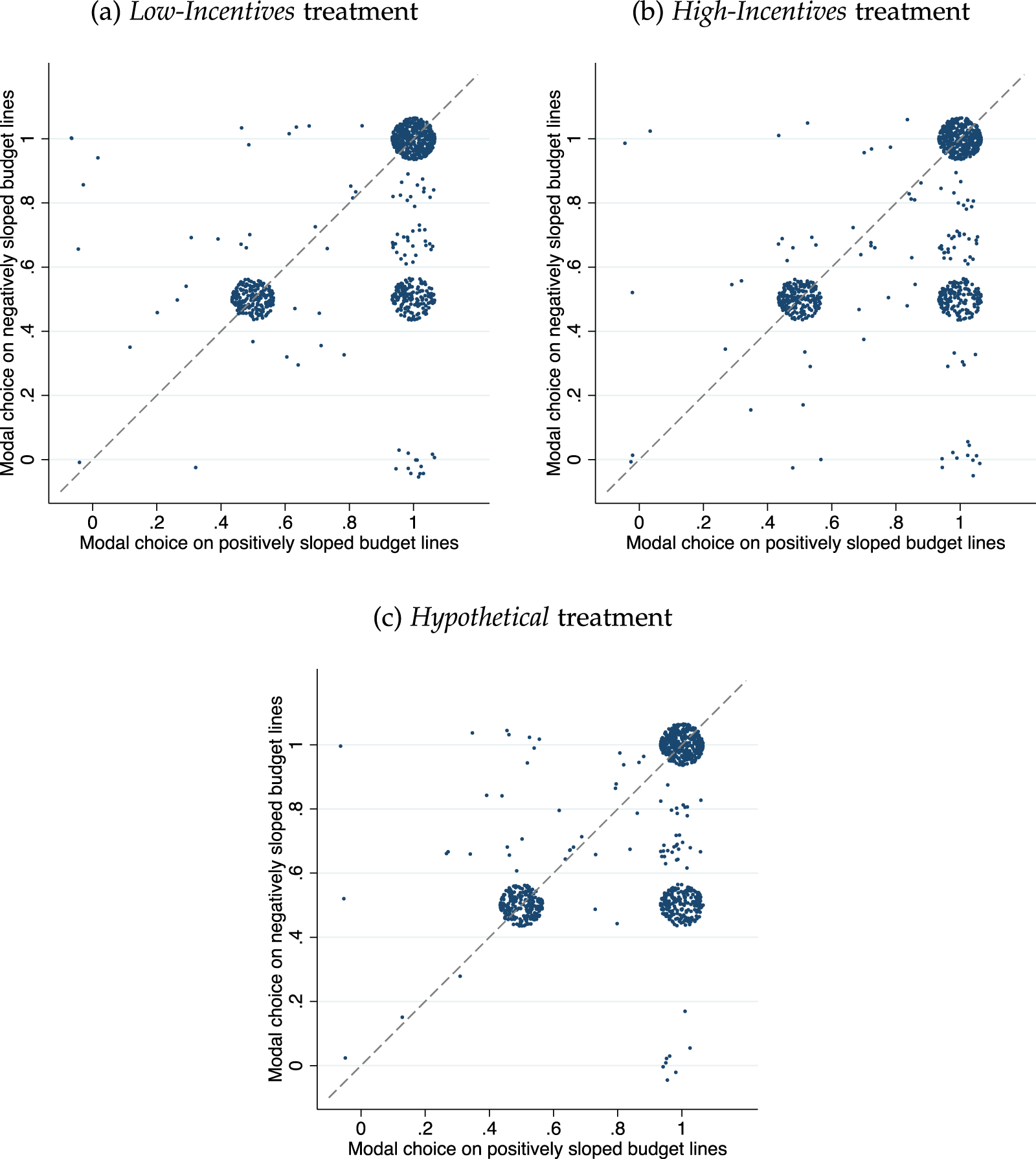
While we explored the distribution of modal choices separately for positively and negatively sloped budget lines in Figure 3, it is also instructive to examine their joint distribution. In Figure 4, we depict subjects’ modal choice on both positively sloped ( $x$-axis) and negatively sloped (
 $y$-axis) budgets in each treatment – where each dot represents a subject. The figure reveals the existence of the same three distinct behavioral agglomerations across all three treatments:
(i) The first behavioral agglomeration is located at
 $z = 0.5$ for both positively and negatively sloped budget lines. In this behavioral agglomeration, individuals tend to predominantly choose the payoff-equalizing allocation, both on positively and on negatively sloped budget lines. This behavioral pattern, which is suggestive of a preference for equality, characterizes roughly 23% of the subjects in the Low-Incentives treatment, 25% in the High-Incentives treatment, and 27% of the individuals in the Hypothetical treatment.
(ii) The second behavioral agglomeration is located at
$z = 1$ for positively sloped budget lines and
$z = 0.5$ for negatively sloped budget lines. These individuals are characterized by a tendency to choose the payoff-equalizing allocation on negatively sloped budget lines, while at the same time predominantly choosing the own-payoff maximizing allocation on positively sloped budget lines – suggesting that these individuals have altruistic concerns for the worse off but tend to be unwilling to reduce the payoff of others for the sake of equality. This agglomeration comprises roughly 18% of the individuals in the Low-Incentives treatment, 20% in the High-Incentives, and 22% of subjects in the Hypothetical treatment.(iii) The third behavioral agglomeration is located at
$z = 1$ for both positively and negatively sloped budget lines. These participants tend to predominantly maximize their own payoffs, with little consideration for the payoffs of others. These predominantly selfish subjects comprise roughly 49% of the subjects in the Low-Incentives treatment, 44% in the High-Incentives treatment, and 42% of the individuals in the Hypothetical treatment.


Descriptive evidence on subjects’ modal choices

Fig. 4 Long description
The image A showing the title “(a) Low-Incentives treatment”. The horizontal axis label reads “Modal choice on positively sloped budget lines”. The vertical axis label reads “Modal choice on negatively sloped budget lines”. The horizontal axis shows tick labels 0, point 2, point 4, point 6, point 8, 1. The vertical axis shows tick labels 0, point 2, point 4, point 6, point 8, 1. A dashed diagonal line runs from near the lower-left corner toward the upper-right corner. Points appear as small filled circles, with three dense circular clusters: one centered near horizontal axis point 5 and vertical axis point 5, one centered near horizontal axis 1 and vertical axis 1 and one centered near horizontal axis 1 and vertical axis point 5. The image B showing the title “(b) High-Incentives treatment”. The horizontal axis label reads “Modal choice on positively sloped budget lines”. The vertical axis label reads “Modal choice on negatively sloped budget lines”. The horizontal axis shows tick labels 0, point 2, point 4, point 6, point 8, 1. The vertical axis shows tick labels 0, point 2, point 4, point 6, point 8, 1. A dashed diagonal line runs from near the lower-left corner toward the upper-right corner. Points appear as small filled circles, with three dense circular clusters: one centered near horizontal axis point 5 and vertical axis point 5, one centered near horizontal axis 1 and vertical axis 1 and one centered near horizontal axis 1 and vertical axis point 5. The image C showing the title “(c) Hypothetical treatment”. The horizontal axis label reads “Modal choice on positively sloped budget lines”. The vertical axis label reads “Modal choice on negatively sloped budget lines”. The horizontal axis shows tick labels 0, point 2, point 4, point 6, point 8, 1. The vertical axis shows tick labels 0, point 2, point 4, point 6, point 8, 1. A dashed diagonal line runs from near the lower-left corner toward the upper-right corner. Points appear as small filled circles, with three dense circular clusters: one centered near horizontal axis point 5 and vertical axis point 5, one centered near horizontal axis 1 and vertical axis 1 and one centered near horizontal axis 1 and vertical axis point 5.
Altogether, the results suggest that individuals’ choices are strikingly similar at the descriptive level, irrespective of whether subjects’ choices in the money allocation task are incentivized, and irrespective of the size of the financial stakes.Footnote 25 While informative, this descriptive approach also has limitations. For example, it only considers subjects’ modal choices and it ignores subjects with non-unique modes. Moreover, this analysis only suggests the existence of behavioral types, but it does not unambiguously assign all individuals to types. For these reasons, we turn to a more rigorous approach in the next section.
4.2. Cluster analysis: do monetary incentives affect the distribution of social preferences?
Do incentives affect the distribution of social preference types in the population? To answer this question, we now turn to a more rigorous analysis that assigns subjects to types on the basis of their choices in the money allocation task. To that end, we apply a Bayesian nonparametric approach – the DP-means clustering algorithm (Kulis & Jordan, Reference Kulis and Jordan2012). This algorithm groups individuals into clusters according to their behavioral similarities. In our context, clusters are based on subjects’ 12 distributional choices (Figure 1), and similarity is measured by “how close” an individual’s allocation profile is to the average allocation of a cluster. Ultimately, individuals are assigned to the cluster whose centroid – i.e., the mean allocation in the 12 distributional choices – is the closest to their own allocation profile in the 12-dimensional space of interest. We describe the formalism of the DP-means algorithm in greater detail in Appendix E.
An important aspect of the DP-means approach is that it enables the identification of preference types without committing to a pre-specified number of different preference types. Moreover, this approach does neither require an ex-ante specification or parameterization of types, nor does it presume a specific error structure. This means that it remains ex-ante agnostic about key distributional assumptions, and it does not constrain heterogeneity to lie within a predetermined set of models or parameter space.Footnote 26 Moreover, the DP-means algorithm allows for all possible type partitions of the data spanning from a representative agent (i.e. a single data-generating process) up to as many types as there are individuals in the population (i.e. n data-generating processes).
We run the DP-means algorithm separately on each treatment. We display the distribution of clusters identified by the DP-means in Table 1.Footnote 27 Consistent with the results of the descriptive analysis, we find that three clusters emerge in each experimental group. The distribution of these clusters is remarkably similar across treatments, with each cluster comprising roughly one third of the population. This result is confirmed by a  $\chi^2$-test, which cannot reject the null hypothesis that the assignment to clusters is independent of the treatments (
 $p = 0.255$).
Type distributions identified using clustering analysis

Table 1 Long description
The table reports the percentage of individuals assigned to three behavior-based clusters under low-incentives, high-incentives, and hypothetical conditions. In every treatment, the predominantly selfish cluster has the highest share, ranging from 34.02 percent in high-incentives to 37.92 percent in low-incentives. Inequality averse individuals make up 31.74 percent in low-incentives, 35.09 percent in high-incentives, and 32.87 percent in hypothetical. Altruistic individuals are close to one-third in each treatment, at 30.34 percent, 30.89 percent, and 32.67 percent respectively. Cluster labels reflect an interpretation of typical behavior from the clustering analysis rather than directly observed motives.
Notes: The table displays the distribution of individuals to the three clusters (in percent) that emerge in our dataset, separately for each treatment. The behavioral interpretation of the clusters (indicated in the left column) is based on the interpretation of each cluster’s typical behavior provided in Figure 5.
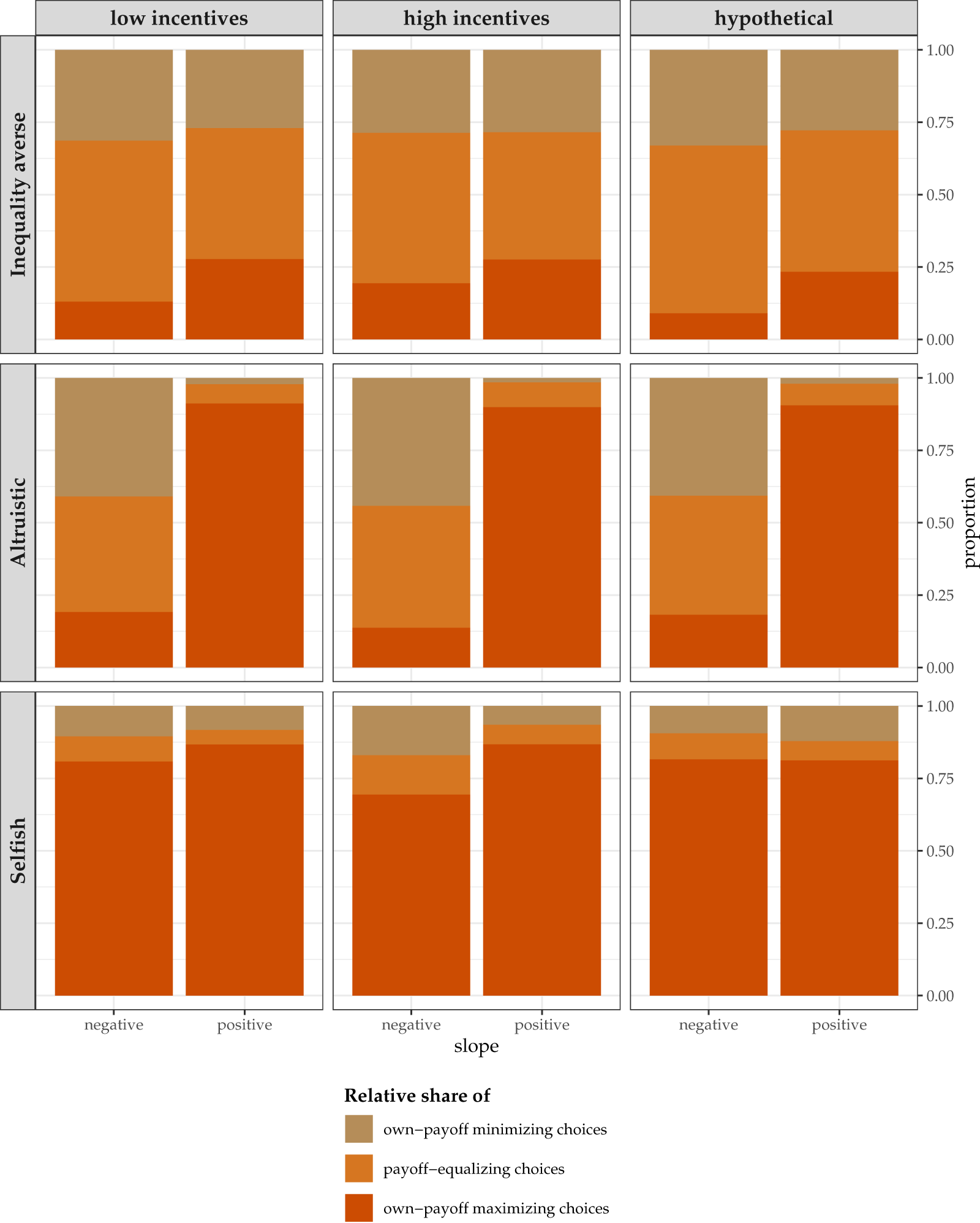
Importantly, the DP-means algorithm does not assign labels to clusters, i.e., it is agnostic as to the behavioral interpretation of types. In order to assign a label to the clusters, one needs to inspect the behavioral characteristics of each cluster identified. To that end, we explore the distribution of choices that characterizes each cluster in each treatment in Figure 5.
The distribution of choices for positively and negatively sloped budget lines in each cluster and each treatment

Fig. 5 Long description
The image shows a set of nine stacked vertical bar graphs arranged in three columns and three rows. Columns are labeled as low incentives, high incentives and hypothetical. Rows are labeled as Inequality averse, Altruistic and Selfish. Each graph contains two bars representing negative and positive slopes. The vertical axis is labeled proportion, ranging from 0.00 to 1.00. The legend indicates three choice types: own-payoff minimizing, payoff-equalizing and own-payoff maximizing. In the Inequality averse row, payoff-equalizing choices dominate across all conditions and both types of budget lines In the Altruistic row, own-payoff minimizing choices and payoff-equalizing choices take up the largest shares for negatively sloped budget lines, while own-payoff maximizing choices dominate for positively sloped budget lines. In the Selfish row, own-payoff maximizing choices dominate for both types of budget lines..
The figure reveals that subjects assigned to Cluster 1 mainly select payoff-equalizing allocations both on negatively sloped and positively sloped budget lines. They thus exhibit a willingness to pay to reduce inequality, both when this involves increasing the payoff of those worse off (negatively sloped budget lines) and decreasing the payoff of those better off (positively sloped budget lines). This behavior is consistent with models of inequality aversion (Bolton & Ockenfels, Reference Bolton and Ockenfels2000; Fehr & Schmidt, Reference Fehr and Schmidt1999) and we therefore assign the label “inequality averse” to this cluster.
Individuals assigned to Cluster 2 display a strikingly different form of other-regarding behavior. They are also willing to pay in order to increase the payoff of those worse off (negatively sloped budget lines), but they are generally unwilling to pay to decrease the payoff of those better off (positively sloped budget lines). They therefore display a tendency to forego own payoff when this benefits the poor, but this willingness to pay vanishes almost entirely when equalizing payoffs would entail reducing the income of those who are better off. This behavioral pattern is consistent with altruistic concerns for the worse off (Charness & Rabin, Reference Charness and Rabin2002) and with altruistic other-regarding behavior that incorporates an equity-efficiency trade-off (Fisman et al., Reference Fisman, Kariv and Markovits2007, Reference Fisman, Jakiela, Kariv and Markovits2015). We therefore label this behavioral cluster as “altruistic.”
The remaining subjects, assigned to Cluster 3, are characterized by making predominantly own-payoff maximizing choices, irrespective of the choice situation. For this reason, we label these individuals as being “predominantly selfish.”
Together, this clustering analysis reveals two striking findings. First, the behavioral interpretation of the three clusters is consistent across the three treatments. In all our experimental conditions, the same three clusters with a similar behavioral interpretation coexist: inequality averse, altruistic, and predominantly selfish subjects.Footnote 28 Second, irrespective of the presence of monetary incentives and irrespective of the stake sizes, the distribution of types is remarkably stable, i.e., the relative share of types remains roughly the same across experimental conditions. This finding is noteworthy, given that the DP-means algorithm imposes no prior assumptions regarding the behavioral interpretation of types nor their distribution in the population.
Overall, these results suggest that whether or not monetary incentives are used to elicit social preferences does not matter for the identification of qualitatively distinct preference types.
4.3. Structural analysis: do monetary incentives affect the strength of social preferences and the precision of their estimates?
The previous sections revealed that monetary incentives do not affect subjects’ aggregate willingness to pay to increase or decrease the payoff of others (descriptive analysis), nor the distribution of preference types in the population (clustering analysis). But do they affect the strength of individuals’ social preferences and the precision of their estimates? It is possible, for example, that low monetary incentives (or absence thereof) lead subjects to take decisions that make them appear more other-regarding than they are if the monetary stakes were high – which would lead one to overestimate social preferences. Likewise, the absence of incentives might increase the share of participants answering randomly, thereby decreasing the precision of social preference estimates.
To address these questions, we estimate the parameters of a hierarchical Bayesian model of social preferences (Fehr & Schmidt, Reference Fehr and Schmidt1999) separately for subjects in different treatments. Specifically, we structurally estimate the following model in each treatment:
 \begin{equation*}
V_{i}\left(w_{ij} \right) = w^{s}_{ij} - \alpha_{i}\max\left\{w^{o}_{ij} - w^{s}_{ij}, 0\right\} - \beta_{i}\max\left\{w^{s}_{ij} - w^{o}_{ij}, 0\right\}
\end{equation*}
where  $w_{ij}= \left(w^{s}_{ij}, w^{o}_{ij}\right)$ corresponds to individual
 $i$’s decision on budget line
 $j$ on how to allocate money between herself (superscript
 $s$ for self) and the other person (superscript
 $o$ for other),
 $\alpha_{i}$ denotes aversion towards disadvantageous inequality (behindness aversion) and
 $\beta_{i}$ denotes aversion towards advantageous inequality (aheadness aversion).Footnote 29
4.3.1. The effects of monetary incentives on the strength of social preferences
We depict the mean values and standard deviations of the estimated structural parameters, separately by treatment, in Table 2. The average level of aversion to disadvantageous inequality ( $\alpha$) is 0.219 in the Low-Incentives treatment and 0.278 in the High-Incentives treatment, i.e., stake size does not significantly affect average levels of behindness aversion (
 $p=0.101$). In contrast, we estimate a considerably higher average
 $\alpha$-parameter of 0.368 for individuals in the Hypothetical treatment, i.e., aversion to disadvantageous inequality in the Hypothetical treatment is on average 68.0% higher than under low stakes (
 $p \lt 0.01$), and 32.4% higher than under high stakes (
 $p=0.024$). These degrees of aversion to disadvantageous inequality are quantitatively sizable. For example, a subject with an
 $\alpha$ of 0.278 (High-Incentives) is willing to pay up to 21.75 cents to decrease the payoff of those ahead by one dollar. In contrast, the estimates from the Hypothetical treatment imply a maximum willingness to pay of up to 26.9 cents, and of up to 18 cents in the Low-Incentives treatment.Footnote 30
The results are somewhat similar when we turn to aversion to advantageous inequality. There too, the highest average  $\beta$ is in the Hypothetical treatment (0.744), which is 21.4% higher than in the Low-Incentives treatment (0.613, test of the difference:
 $p \lt 0.01$) and about 4.5% higher than in the High-Incentives treatment (0.712, test of the difference:
 $p=0.487$). In terms of magnitude, a subject with a
 $\beta$ of 0.712 (High-Incentives) is willing to pay up to 2.47 dollars to increase the payoff of someone worse off by one dollar, as opposed to a willingness to pay of 1.58 in the Low-Incentives treatment and of 2.90 in the Hypothetical treatment.Footnote 31
Summary statistics across treatments

Table 2 Long description
The table reports mean values and standard deviations for two measures across three conditions: low incentives, high incentives, and hypothetical. For the alpha measure, the mean increases from 0.219 in low incentives to 0.278 in high incentives and 0.368 in hypothetical, with standard deviations rising from 0.775 to 0.843 to 0.956. For the beta measure, the mean increases from 0.613 to 0.712 to 0.744 across the same conditions. Its standard deviation is about 0.965 in low incentives and 0.961 in high incentives, then increases to 1.124 in the hypothetical condition. Overall, both measures show higher average values as incentives increase and are highest under the hypothetical condition. Variation is broadly similar between low and high incentives, while the hypothetical condition shows the greatest spread, especially for the beta measure.
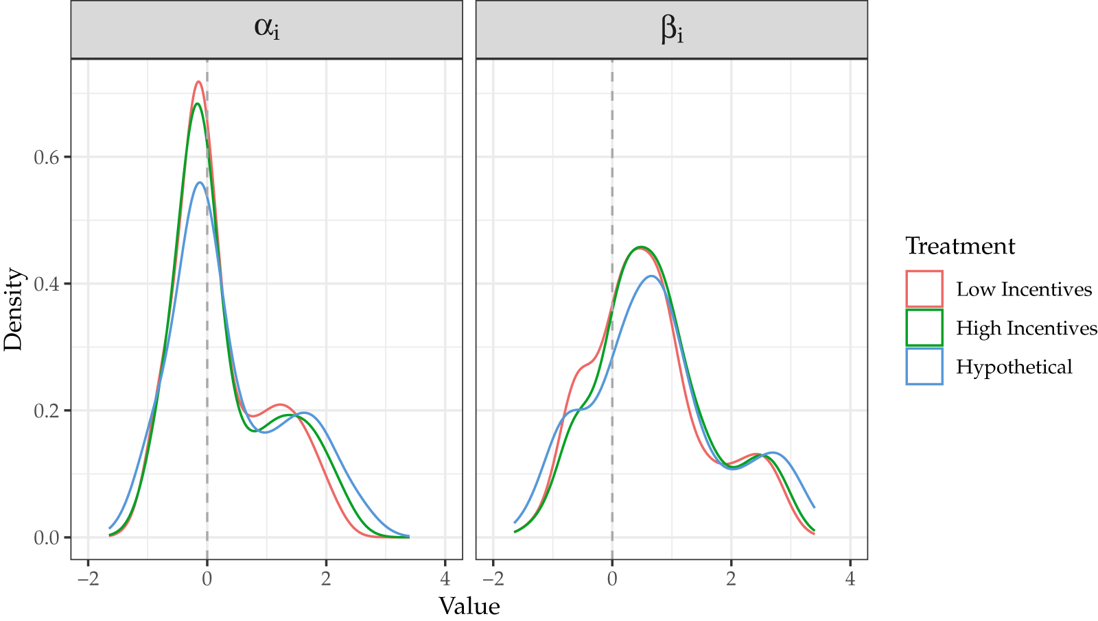
Do the distributions of  $\alpha$ and
 $\beta$ differ across treatments? We depict their probability density function in Figure 6, and a series of pairwise KS tests of equality in distributions in Table 3.Footnote 32
Distribution of structurally estimated parameters

KS test  $p$-values with Holm (Reference Holm1979) correction

Table 3 Long description
The table reports Kolmogorov–Smirnov test p-values for pairwise comparisons of distributions, adjusted for multiple testing using the Holm method. It compares Low Incentives, High Incentives, and Hypothetical conditions for two parameters labeled alpha and beta. Low Incentives versus High Incentives has p-value 0.106 for alpha and 0.034 for beta, suggesting weaker evidence of a difference for alpha than for beta. Low Incentives versus Hypothetical shows p-value 0.001 for both alpha and beta, indicating very strong evidence of differences for both parameters. High Incentives versus Hypothetical shows p-value 0.032 for alpha and 0.001 for beta, again indicating stronger evidence for beta than for alpha.
Consistent with our discussion above, we find that the distributions of  $\alpha$ and
 $\beta$-parameters are relatively similar in the Low- and High-Incentives treatment, but that the Hypothetical treatment significantly shifts both distributions to the right.Footnote 33 Indeed, while stake sizes do not significantly affect the distribution of individuals’ estimated
 $\alpha$-parameters (Low- vs. High-Incentives:
 $p=0.106$), we can reject the null hypotheses that individuals in the Hypothetical treatment have similar distributions to those in the two incentivized treatments (Low-Incentives vs. Hypothetical:
 $p=0.001$; High-Incentives vs. Hypothetical:
 $p=0.032$).
Turning to the distributions of  $\beta$, we again most strongly reject the null hypothesis of equality in distribution when comparing the Hypothetical with the Low-Incentives treatments (
 $p=0.001$), and the Hypothetical with the High-Incentives treatment (
 $p=0.001$). Interestingly, we can also reject the null hypothesis of equality in distributions between the Low- and the High-Incentives treatments, although the significance level of this test is lower (
 $p=0.034$).
These results point towards a common conclusion: while the size of the monetary stakes does not play a large role in the strength of social preferences, whether or not monetary incentives are used matters. Specifically, we find that the social preference parameters are consistently larger – i.e., possibly overestimated – in the absence of monetary incentives.
How do the different preference types identified in Section 4.2 relate to structural parameters of  $\alpha$ and
 $\beta$? In Figure D.4 in Appendix D.3, we shed light on this question by examining the distributions of these parameters separately by preference type.
This analysis reveals that the treatment differences highlighted above are mainly driven by the inequality-averse subjects (Cluster 1). Inequality-averse subjects display a strong and significant rightward shift in the distribution of social preferences parameters in the Hypothetical treatment. In other words, inequality averse subjects respond to the lack of monetary incentives with larger values of  $\alpha$ and
 $\beta$. For the other two preference types, we do not find such strong treatment differences.
4.3.2. The effects of monetary incentives on the precision of structural estimates
To assess whether monetary incentives improve the reliability of our preference estimates, we use the parameter estimates from the structural hierarchical Bayesian models of each treatment and extract, for every individual, the posterior standard deviation of the two behavioral parameters  $\alpha_i$ and
 $\beta_i$. These within-person dispersions quantify the precision with which the model recovers each individual’s preferences: the narrower the posterior, the more informative the data. Comparing the median posterior standard deviation across incentive conditions therefore provides a direct test of whether incentivized tasks yield tighter, higher-quality parameter estimates than non-incentivized ones, independent of the heterogeneity in preferences between individuals. Table 4 presents the results. The precision of the estimates improves substantially when moving from hypothetical to incentivized measures of social preferences. Hence, using financial incentives increases the precision with which social preference parameters are estimated (compared to hypothetical choices).
Median posterior standard deviation of individuals’ preference parameters by treatment condition

Table 4 Long description
The table reports the median posterior standard deviation, a measure of uncertainty, for individuals’ preference parameters across three treatment conditions. For alpha, uncertainty is 0.238 in Low-Incentives, 0.224 in High-Incentives, and 0.310 in Hypothetical. For beta, uncertainty is 0.221 in Low-Incentives, 0.196 in High-Incentives, and 0.290 in Hypothetical. In both parameters, the Hypothetical condition shows the greatest uncertainty and the High-Incentives condition shows the least. Low-Incentives falls between these two for both alpha and beta.
Overall, this structural analysis reveals an important lesson that was not identified in the descriptive nor in the clustering analyses. With hypothetical stakes, the estimated strength of social preferences is larger than with monetary incentives – suggesting that they are overestimated. This result is primarily driven by individuals identified as being inequality averse in the clustering analysis. Moreover, the precision with which individuals’ preference parameters are estimated is lower under hypothetical stakes. In contrast, the magnitude and the precision of the parameters estimated in the Low- and High-Incentives treatments are similar.
4.4. Do monetary incentives affect the measurement of students’ social preferences?
While our main interest is to understand whether and how monetary incentives affect measures of social preferences in the general population, it is also instructive to investigate how they affect students. To shed light on this issue, we reproduce the analysis above, focusing on our sample of 495 students (for details on the sample, see Section 2.3). Because this analysis is not our main focus, we only summarize it here and relegate the details to Appendix F.Footnote 34 Moreover, note that this analysis is less well-powered than our analysis for the general population. As such, it should be interpreted with greater caution.
At the descriptive level, we find that the distributions of students’ modal choices are essentially unaffected by the treatments: The majority of students predominantly select either the payoff-equalizing ( $z = 0.5$) or the own-payoff maximizing allocations (
 $z = 1$), irrespective of whether their decisions are incentivized (and by how much). Moreover, none of the six KS tests for pairwise comparisons can reject the null hypothesis of equality in distributions between conditions.
Turning to the clustering analysis, we again find that heterogeneity in preferences is best captured by three types – an inequality averse, an altruist, and a predominantly selfish type – in the Low-Incentives and in the Hypothetical treatments. However, the DP-means algorithm does not identify a stable three-type clustering in the High-Incentives treatment.Footnote 35 Interestingly, for those treatments for which we identify three clusters, the assignment of students to types is quite responsive to incentives: in the Hypothetical treatment, 76.83% of the subjects are assigned to one of the other-regarding clusters (i.e., either altruistic or inequality averse), whereas only 55.07% are assigned to such a cluster when money is at stake (Low-Incentives treatment). In other words, students are more likely to be assigned to the selfish type when monetary incentives are used.
The impact of incentives on the structurally estimated preference parameters is less clear-cut for students compared to the general population. While monetary incentives reduce the strength of social preferences in the general population, the results for the student sample are more mixed. Specifically, while we also find that the distribution of estimated aversion to advantageous and disadvantageous inequality is higher under Hypothetical incentives than under Low-Incentives, we find that it is the highest under High-Incentives. This suggests that stronger monetary incentives yield stronger social preferences in the student sample. These results should be taken with a grain of salt, however, as the precision with which these parameters are estimated is substantially lower than in the general population.Footnote 36
Summarizing, the results from the students’ sample are broadly consistent with those of the general population. While we identified a few inconsistencies between these two different samples, we cannot rule out that they are due to the smaller sample size (and associated greater estimation uncertainty) in the student sample.
5. Concluding remarks
Using a pre-registered online experiment with a representative sample of the US population, we examined whether the use of monetary incentives and variations in stake size matter for the identification of social preferences. We explored this question in three steps: at the descriptive level of subjects’ modal choices, at the level of qualitatively distinct preference types, and at the level of individuals’ structurally estimated social preference parameters.
Our results show that the use of monetary incentives, as well as the size of the stakes, have little impact on choices at the descriptive levels, as well as for the identification of qualitatively distinct preference types. They appear to matter, however, for the quantitative identification of the strength and the precision of social preferences. In particular, our structural analysis reveals that the social preferences of the general population are likely overestimated when elicited with hypothetical stakes.
These results suggest that whether or not incentives should be used to elicit social preferences depends on the specifics of the research question at hand. If one is solely interested in having a rough, descriptive measure of social preferences at the aggregate level, or if one wants to identify qualitatively distinct preference types, then relying on hypothetical stakes might suffice. However, if one is interested in making a quantitative assessment of subjects’ other-regardingness, e.g., in order to make quantitative predictions, then our results suggest that using monetary incentives is advisable, as hypothetical stakes appear to yield an overestimation of inequality aversion. However, we find no evidence that using a larger stake size improves the identification of social preferences, consistent with two meta-analyses showing that larger stakes have little to no effect on decisions in dictator games (Engel, Reference Engel2011; Larney et al., Reference Larney, Rotella and Barclay2019).
Supplementary material
The supplementary material for this article can be found at https://doi.org/10.1017/eec.2026.10054.
Acknowledgements
The “ⓡ” symbol indicates that the authors’ names are in certified random order. Ernst Fehr acknowledges the support from the Research Priority Program of the University of Zurich on Equality of Opportunity. Thomas F. Epper acknowledges the support from the Métropole Européenne de Lille (MEL).
Replication package
The replication package for this paper is available at https://doi.org/10.17605/OSF.IO/3G8D5.









 Open access

