





1. Introduction
1.1. The stationary rope with a parallel electric field
Magnetic flux ropes are coherent current-carrying structures in which magnetic field lines wind helically about a common axis. In the cylindrical description commonly used for laboratory and astrophysical ropes, the magnetic field is tangent to nested cylinders,
 \begin{align} \boldsymbol B = B_{\phi }(r)\,\hat {\boldsymbol e}_{\phi } + B_{\chi }(r)\,\hat {\boldsymbol e}_{\chi }, \end{align}
where
 $\phi$
and
 $\chi$
denote the azimuthal and axial coordinates. This geometry includes the screw pinch of laboratory plasma physics, the large-aspect-ratio description of loop-voltage-driven plasma columns, and local models of solar and interplanetary flux ropes (Lundquist Reference Lundquist1950; Gold & Hoyle Reference Gold and Hoyle1960; Titov & Démoulin Reference Titov and Démoulin1999; Freidberg Reference Freidberg2014; Filippov et al. Reference Filippov, Martsenyuk, Srivastava and Uddin2015). Magnetic twist, electric current, stress and helicity are closely connected in all of these settings.
Magnetic twist and principal-sector multiplicity are distinct. A single rank-two electromagnetic two-form
 $F$
can already describe a flux rope with helical magnetic field lines. Here an electromagnetic contribution means one complete rank-two two-form, such as
 $G$
or
 $H$
in the decomposition introduced later; it is neither a coordinate component nor an independent physical electromagnetic field or material flux tube. The two-sector description becomes relevant here because the total field is rank four, equivalently
 $F\wedge F\neq 0$
or
 $\boldsymbol E\boldsymbol{\cdot }\boldsymbol B\neq 0$
, rather than merely because its magnetic field is twisted. For a stationary purely magnetic rope, introduce the flux function
 $ \varPsi '(r)=rB_{\chi }(r).$
The corresponding magnetic two-form is
 \begin{align} F_{\textrm {ideal}} = {\rm d}\varPsi \wedge {\rm d}\phi - B_{\phi }(r)\,{\rm d}r\wedge {\rm d}\chi . \end{align}
It is rank two, or simple, because
 $ F_{\textrm {ideal}}\wedge F_{\textrm {ideal}}=0.$
Electromagnetically, this means that its electric and magnetic parts satisfy
 $\boldsymbol E\boldsymbol{\cdot } \boldsymbol B=0.$
The term simple will be used subsequently only in this algebraic sense. It does not mean weakly twisted and it does not by itself impose all of the dynamical assumptions of ideal MHD.
The Gold–Hoyle rope (Gold & Hoyle Reference Gold and Hoyle1960),
 \begin{align} B_{\chi } = \frac {B_{0}}{1+q^{2}r^{2}}, \qquad B_{\phi } = qrB_{\chi }, \end{align}
provides a useful example. Substitution into (1.2) gives
 \begin{align} F_{\textrm {GH}} = {\rm d}\varPsi \wedge \left ( {\rm d}\phi -q\,{\rm d}\chi \right ). \end{align}
Thus, a strongly helical magnetic field can still be represented by a single rank-two field. Its field-line geometry can be described using Euler or flux potentials in the usual way (Newcomb Reference Newcomb1958; Stern Reference Stern1970).
The class studied in this paper is distinguished by a non-vanishing parallel electric field,
 \begin{align} \boldsymbol E\boldsymbol{\cdot }\boldsymbol B\neq 0. \end{align}
Parallel electric fields are observed in reconnection-generated and kinetic-scale flux ropes, where they accompany field-aligned currents, particle acceleration and electromagnetic energy conversion (Wilmot-Smith, Hornig & Pontin Reference Wilmot-Smith, Hornig and Pontin2009; Zhong et al. Reference Zhong, Tang, Zhou, Deng, Pang, Paterson, Giles, Burch and Torbert2018; Du et al. Reference Du, Fu, Cao, Grigorenko, Chen, Wang, Guo, Xu and Fu2025). They can also be maintained by externally imposed voltages in stationary resistive plasma columns.
In electromagnetic two-form language,
 $ \boldsymbol E\boldsymbol{\cdot }\boldsymbol B\neq 0 \Longleftrightarrow F\wedge F\neq 0.$
The field is then rank four, or non-degenerate, and cannot be represented by a single simple two-form. This is the algebraic reason that the present non-ideal rope requires two rank-two contributions.
This statement concerns the particular non-ideal class satisfying (1.5). We do not claim that every departure from ideal MHD must have
 $\boldsymbol E\boldsymbol{\cdot }\boldsymbol B\neq 0$
. Degenerate ideal and force-free electromagnetic fields, including their Euler-potential descriptions, are treated extensively in the existing literature (Uchida Reference Uchida1997; Gralla & Jacobson Reference Gralla and Jacobson2014; Gralla & Iqbal Reference Gralla and Iqbal2019).
1.2. Physical meaning of the two principal sectors
A rank-four electromagnetic field possesses two mutually metric-orthogonal principal planes, one timelike and one spacelike. Accordingly, it can be written locally as
 \begin{align} F=G+H, \qquad H=\rho {\star G}, \end{align}
where
 $G$
and
 $H$
are rank-two fields supported on the two principal planes and
 $\rho$
is their relative amplitude. The principal planes are selected by the electromagnetic field and the space–time metric; their orthogonality is therefore not an additional flux-rope modelling assumption (Penrose & Rindler Reference Penrose and Rindler1984).
We call
 $G$
and
 $H$
the two principal sectors of
 $F$
. A sector is not a coordinate component of
 $ F$
, and the two sectors are not simply the electric and magnetic parts measured by an observer. Each is a complete rank-two electromagnetic contribution and therefore satisfies
 $\boldsymbol E_G\boldsymbol{\cdot }\boldsymbol B_G =\boldsymbol E_H\boldsymbol{\cdot }\boldsymbol B_H=0$
. Relative to a chosen observer, it contributes its own electric and magnetic fields, either of which may vanish in a special limit. Nevertheless, the completed field may satisfy
 $\boldsymbol E\boldsymbol{\cdot }\boldsymbol B = \boldsymbol E_G\boldsymbol{\cdot }\boldsymbol B_H + \boldsymbol E_H\boldsymbol{\cdot }\boldsymbol B_G \neq 0$
. The non-ideal invariant is therefore produced by cross-sector pairings, rather than by either rank-two contribution in isolation. The physical field decomposition is illustrated in figure 1.
Physical interpretation of the stationary cylindrical principal pair. (a) The driven annular rope before axial compactification. The blue and red helices indicate the magnetic directions contributed by the two rank-two sectors
 $G$
and
 $H$
, respectively; they are not separate material flux tubes. The azimuthal electromotive period and the axial electric drive are maintained externally; after the identification of § 4,
 $L_{\chi }k_{2}$
becomes the axial loop electromotive period. The resulting cross-sector coupling permits
 $\boldsymbol E\boldsymbol{\cdot }\boldsymbol B\neq 0$
. (b) Local tangent-plane interpretation of the metric-conjugate pair. Each sector is rank two, so
 $\boldsymbol E_I\boldsymbol{\cdot }\boldsymbol B_I=0$
, but
 $\boldsymbol E\boldsymbol{\cdot }\boldsymbol B =hr(|\boldsymbol B_{G}|^{2}-|\boldsymbol E_{G}|^{2})$
. The non-zero invariant of the completed field is produced by the crossed pairings between the two sectors.

Figure 1. Long description
The two-panel schematic explains how the two principal electromagnetic sectors combine in the stationary annular rope. Panel (a) shows a hollow cylinder before axial compactification. A blue solid helix B G and a red dashed helix B H wind in opposite senses and represent magnetic directions contributed by the sectors, not separate material flux tubes. A cyan circular arrow at the top marks the externally maintained azimuthal electromotive period, a purple upward arrow marks the axial electric drive, and an orange outward arrow marks radial Poynting flow. Opposed blue and red arrows at the lower boundary indicate that the sector non-closures cancel, d G plus d H equals zero. Panel (b) unwraps the azimuthal-axial tangent plane at fixed radius. The blue B G vector is mainly azimuthal and the red B H vector mainly axial; they are perpendicular and have opposite pitches. Green E and black B are the total electric and magnetic fields. Labels show the crossed pairings B H parallel to E G and B G parallel to E H, and the pitch product p G times p H equals minus r squared. Each sector separately has zero E I dot B I, while the crossed pairings permit non-zero total E dot B.
The decomposition is algebraic and does not by itself impose Maxwell’s equations. The physical field must also obey the homogeneous Maxwell equations,
 $ {\rm d}F={\rm d}G+{\rm d}H=0.$
In the configurations studied herein, the two sectors are generally not closed separately:
 \begin{align} {\rm d}G=-{\rm d}H\neq 0. \end{align}
Neither
 ${\rm d}G$
nor
 ${\rm d}H$
represents a physical magnetic-monopole current. They are internal bookkeeping quantities associated with the variation of the two sector planes; only their cancellation in the total field is physical.
The integrability conditions for the individual sectors, the obstruction to such a cancellation when both principal kernels are Frobenius integrable and the general local principal-completion problem are developed in a companion paper (Kim Reference Kim2026a ). In particular, a non-trivial cancellation of the form (1.7) requires at least one principal kernel to be non-integrable. In physical terms, at least one sector fails to define a foliation by coherent flux surfaces. On the regular two-helix branch of the radially dependent cylindrical ansatz used here, this non-integrability is diagnosed by radial shear of the sector’s helical direction. We refer to the resulting sector-plane non-integrability as anholonomy.
These general mathematical results are not rederived here. Instead, we use them to determine what the principal-sector geometry implies for the magnetic pitch, electric field, current, material support, Poynting transport and helicity of a stationary cylindrical plasma rope.
1.3. Model assumptions and scope
The physical model developed herein is a stationary, axisymmetric plasma column in flat cylindrical spacetime. The radial domain is a finite annulus
 $r_{1}\leqslant r\leqslant r_{2}$
; all profile functions depend only on
 $r$
, and both the electric and magnetic fields are tangent to the cylinders
 $r=\mathrm{const.}$
. The two principal contributions are specified directly as a finite metric-conjugate pair. No seed field, perturbative deformationor proximity to a reference flux tube is assumed.
Within this ansatz, imposing the homogeneous Maxwell equations
 ${\rm d}F=0$
produces the stationary locking relation of Proposition1. This relation is specific to the cylindrical symmetry, radial dependence and principal-pair form introduced in § 2.1; it is not claimed for arbitrary flux ropes. The assumptions required for the successive results are summarised in table 1.
Scope of the results and assumptions required at each stage.

Table 1. Long description
The table has two columns, Result and Assumptions required, and five rows. Row 1, Local principal decomposition: this requires a rank-four electromagnetic field on a Lorentzian four-manifold and is independent of cylindrical symmetry and plasma modelling. Row 2, Stationary Maxwell locking: this additionally requires flat cylindrical spacetime, stationarity, axisymmetry, radial profile dependence and the principal-pair ansatz of Section 2.1. Row 3, Current and material support: the current follows from the inhomogeneous Maxwell equation; pressure balance and the resistive realization also require the constitutive and mechanical assumptions of Sections 3.3 and 3.4, which give admissible examples rather than a unique plasma closure. Row 4, Winding and generalized helicity: this additionally requires a finite annulus with the periodic axial identification chi equivalent to chi plus L chi, imposed only in Sections 4 and 5. Row 5, Localized intersection formula, Equation 5.26: this further uses the periodic geometry and a formal delta-shell limit; the limit exposes the intersection pairing but is not claimed to be a smooth principal-locked equilibrium.
The axial direction is therefore not assumed to be periodic in deriving the locking relation, the observable fields or their local material support. Before the identification, the system may be interpreted as a straight finite plasma column with an axial voltage maintained at its ends. Periodicity is introduced only for the winding and helicity analysis, where it provides a large-aspect-ratio surrogate for toroidal closure without including toroidal curvature.
The electromagnetic profiles obtained herein belong to the familiar class of stationary cylindrical Maxwell fields. The new result is their organisation into two principal contributions: Maxwell closure becomes an algebraic locking between the two helical directions, the observable magnetic profile and the imposed electric drives. This organisation permits reconstruction of the principal variables and relates their local radial pitch shear to the global helicity structure of the periodically identified annulus.
2. Stationary cylindrical principal pair and Maxwell locking
2.1. The stationary cylindrical principal pair
We work in cylindrical coordinates
 $x^{a}=(t,r,\phi,\chi )$
with the flat metric
 \begin{align} {\rm d}s^{2} = -{\rm d}t^{2} +{\rm d}r^{2} +r^{2}{\rm d}\phi ^{2} +{\rm d}\chi ^{2}, \end{align}
and orientation
 $\varOmega :={\rm d}t\wedge {\rm d}r\wedge {\rm d}\phi \wedge {\rm d}\chi \gt 0.$
The configuration is stationary and cylindrically symmetric, and all profile functions depend only on
 $r$
. Both the electric and magnetic fields will be tangent to the cylindrical surfaces.
The general mathematics of metric-conjugate rank-two sectors and Bianchi-closed principal completion is developed by Kim (Reference Kim2026a ). We now specify directly the finite stationary principal pair used throughout the paper. Introduce the one-form legs
 \begin{align} \vartheta _G &:= {\rm d}r+C(r)\,{\rm d}t, & \beta _G &:= B(r)\,{\rm d}\phi +A(r)\,{\rm d}\chi, \end{align}
 \begin{align} \vartheta _H &:= {\rm d}t+C(r)\,{\rm d}r, & \beta _H &:= B(r)\,{\rm d}\chi -r^{2}A(r)\,{\rm d}\phi . \end{align}
The two rank-two sectors are defined by
 \begin{eqnarray} G := \vartheta _G\wedge \beta _G = ({\rm d}r+C\,{\rm d}t) \wedge (B\,{\rm d}\phi +A\,{\rm d}\chi), \end{eqnarray}
 \begin{eqnarray} H := h(r)\,\vartheta _H\wedge \beta _H = h(r) ({\rm d}t+C\,{\rm d}r) \wedge (B\,{\rm d}\chi -r^{2}A\,{\rm d}\phi). \end{eqnarray}
No profile in (2.4) and (2.5) is assumed to be small.
The functions have a direct role in the cylindrical pair. The ratio
 $A/B$
determines the helical direction carried by the first sector,
 $C$
describes a boost-like mixing of its radial and temporal legs, and
 $h$
gives the amplitude of the metric-conjugate sector. The quantity
 $B(r)$
is a reconstruction variable and should not be confused with the magnitude of the observable total magnetic field.
On any interval where
 $B\neq 0$
, we introduce
 \begin{align} a(r):=\frac {A(r)}{B(r)}. \end{align}
The relation of
 $a(r)$
to the observable magnetic pitches is derived in § 3.
The two pairs of legs are mutually metric orthogonal:
 $ g^{-1}(\vartheta _G,\vartheta _H)=0$
and
 $g^{-1}(\beta _G,\beta _H)=0.$
Their norms are
 $g^{-1}(\vartheta _G,\vartheta _G)=1-C^{2}$
,
 $ g^{-1}(\vartheta _H,\vartheta _H)=-(1-C^{2})$
,
 $ g^{-1}(\beta _G,\beta _G)= D/r^{2}$
and
 $ g^{-1}(\beta _H,\beta _H)= D$
, where
 \begin{align} D(r):=B^{2}(r)+r^{2}A^{2}(r). \end{align}
A regular Lorentzian splitting into one spacelike and one timelike principal plane therefore requires
 \begin{align} \fbox {${ C^{2}\lt 1, \qquad D\gt 0. }$} \end{align}
The first condition keeps the radial–temporal mixing subluminal. The second excludes the trivial limit in which the first sector vanishes.
With the orientation chosen here, the Hodge dual of
 $G$
is
 $ \star G = ({1}/{r}) \vartheta _H\wedge \beta _H.$
Consequently,
 \begin{align} \fbox {${ H=hr\,\star G. }$} \end{align}
Thus,
 $G$
and
 $H$
occupy metric-conjugate principal planes, with relative principal amplitude
 $ \rho (r)=hr.$
The total electromagnetic field is
 $ F:=G+H.$
Since both sectors are simple,
 $G\wedge G=H\wedge H=0$
, while
 \begin{align} F\wedge F = 2G\wedge H = 2h(1-C^{2}){\rm D}\varOmega . \end{align}
Subject to (2.8), the total field is therefore rank four wherever
 $h\neq 0$
. The parallel electric field of the completed configuration is produced by the coupling between the two rank-two sectors.
2.2. Maxwell closure and the stationary locking relation
The principal-pair structure does not by itself guarantee that
 $F$
is an admissible electromagnetic field. The homogeneous Maxwell equations require (1.7). For the pair defined here, the exterior derivatives are
 \begin{align} {\rm d}G ={}& -(BC)'\, {\rm d}t\wedge {\rm d}r\wedge {\rm d}\phi -(AC)'\, {\rm d}t\wedge {\rm d}r\wedge {\rm d}\chi, \nonumber \\[3pt] {\rm d}H ={}& (hr^{2}A)'\, {\rm d}t\wedge {\rm d}r\wedge {\rm d}\phi -(h\!B)'\, {\rm d}t\wedge {\rm d}r\wedge {\rm d}\chi . \end{align}
Hence,
 ${\rm d}F=0$
is equivalent to the two radial equations
 $ (hr^{2}A)'=(BC)'$
and
 $(h\!B)'=-(AC)'.$
After one radial integration,
 $ hr^{2}A-BC=k_{1}$
and
 $ h\!B+AC=k_{2},$
where
 $k_{1}$
and
 $k_{2}$
are constants. Using
 $A=aB$
, these equations form a pointwise algebraic system for the two combinations
 $ \eta :=h\!B$
and
 $\varLambda :=BC.$
Solving it gives the central stationary locking relation.
Proposition 1 (Stationary principal-sector locking). Let
 $G$
and
 $H$
be given by (
2.4
) and (
2.5
), with all profiles depending only on
 $r$
. Then,
 $F=G+H$
satisfies
 ${\rm d}F=0$
if and only if
 \begin{align} \fbox {${ h\!B = \dfrac {k_{2}+k_{1}a} {1+r^{2}a^{2}}, \qquad BC = \dfrac {k_{2}r^{2}a-k_{1}} {1+r^{2}a^{2}}, }$} \end{align}
for
 $B \neq 0$
. Thus, the principal-sector amplitude
 $h\!B$
and the radial-mixing combination
 $BC$
are fixed pointwise once the pitch profile
 $a(r)$
, the radial profile
 $B(r)$
and the two drive constants are specified.
The electric interpretation of these constants is given in § 3.2:
 $k_{1}$
fixes the azimuthal electromotive period, whereas
 $k_{2}$
is the axial electric drive before compactification. Thus, within the present stationary cylindrical ansatz, Maxwell closure fixes
 $h\!B$
and
 $BC$
pointwise from
 $a$
,
 $B$
and the two drive constants.
Accordingly, the stationary locking relation can be stated as follows: once the magnetic pitch profile and the two electric drives are specified, Maxwell closure fixes the amplitude of the conjugate principal sector and the radial–temporal mixing at every radius. The locking is algebraic rather than differential after the two Maxwell equations have been integrated.
This result is specific to the stationary, radially dependent cylindrical pair. It is not a general relation for arbitrary flux ropes, nor is it the general kinematic locking relation derived by Kim (Reference Kim2026a ). The latter follows from metric conjugacy before imposing a particular field equation. Equation (2.12) is instead the additional profile locking imposed by the homogeneous Maxwell equations in the present cylindrical geometry. Electric charge and current are determined separately from the inhomogeneous Maxwell equation in § 3.
If
 $k_{1}=k_{2}=0$
, (2.12) gives
 $h\!B=BC=0.$
For
 $B\neq 0$
, this implies
 $h=C=0$
and the field reduces to a single stationary rank-two magnetic sector. A stationary rank-four solution within the present ansatz therefore requires a non-vanishing electric drive. Non-zero
 $k_{1}$
or
 $k_{2}$
is necessary, although the local non-degeneracy condition
 $h\neq 0$
must still be checked throughout the chosen radial domain.
2.3. Radial pitch shear and sector anholonomy
The general relation between principal-sector integrability, anholonomy and Bianchi closure is established by Kim (Reference Kim2026a ). In the present cylindrical pair, the corresponding diagnostics reduce to radial pitch-shear expressions that can be read directly from the profiles.
Using (2.11), one obtains
 \begin{align} \beta _G\wedge {\rm d}G &= -CB^{2}a'\,\varOmega, \qquad \beta _H\wedge {\rm d}H = -h\!B^{2} (r^{2}a)'\varOmega . \end{align}
We therefore define the anholonomies
 \begin{align} \fbox {${ q_G(r) := -CB^{2}a', \qquad q_H(r) := -h\!B^{2} (r^{2}a)'. }$} \end{align}
These quantities measure the failure of the two principal planes to remain integrable as their helical directions vary across the annulus. The pitches are derived in (3.9) later. Thus,
 $q_G$
is controlled by the radial shear of
 $a$
or, equivalently, of the first-sector pitch, while
 $q_H$
is controlled by the radial shear of the conjugate pitch
 $r^{2}a$
.
Pitch shear alone is not sufficient to produce non-zero anholonomy. For the
 $G$
sector, it must be accompanied by non-zero radial–temporal mixing
 $C$
, whereas for the
 $H$
sector, the conjugate amplitude
 $h$
must be non-zero. Assuming
 $B\neq 0$
,
 \begin{align} q_G\neq 0 &\quad \Longleftrightarrow \quad C\neq 0 \quad \text{and}\quad a'\neq 0, \end{align}
 \begin{align} q_H\neq 0 &\quad \Longleftrightarrow \quad h\neq 0 \quad \text{and}\quad (r^{2}a)'\neq 0. \end{align}
This qualification is important: a magnetic pitch may vary radially while the corresponding rank-two sector remains integrable in a degenerate limit such as
 $C=0$
.
Combining (2.14) with the stationary locking relation, both sectors are strictly anholonomic wherever
 $ a'\neq 0$
,
 $ (r^{2}a)'\neq 0$
,
 $k_{2}r^{2}a-k_{1}\neq 0$
and
 $ k_{2}+k_{1}a\neq 0.$
The Lorentzian signature condition (2.8) additionally requires
 $|{k_{2}r^{2}a-k_{1}}/{B(1+r^{2}a^{2})}| \lt 1.$
Limits in which one of the two anholonomy coefficients vanishes remain admissible Maxwell fields; the corresponding sector simply becomes integrable. An explicit regular configuration for which both coefficients remain non-zero throughout a finite annulus is constructed in § 3.5 and Appendix A.
2.3.1. Related non-stationary branch
The algebraic locking relation (2.12) relies on stationarity and radial dependence. A related time-dependent helical branch, in which the radial support is held fixed while the pitch evolves, has been analysed separately by Kim (Reference Kim2026b ). In that branch, Bianchi closure becomes a nonlinear conservation law for the metric-weighted pitch, and compressive profiles may develop finite-time characteristic crossings accompanied by principal-plane anholonomy and current concentration. That dynamical initial-value problem is structurally distinct from the stationary branch considered here and will not be pursued further.
3. Electromagnetic fields, currents and material support
All coefficient functions depend on
 $r$
alone, so the configuration is time independent. It is stationary rather than static: a non-zero radial frame mixing carries a stationary Poynting flux, as quantified in § 3.3. The closure relation determines the electromagnetic field, not its sources. We now use
 ${\rm d}\star F=J_{\textrm {e}}$
to obtain the physical current, and then introduce explicit force-balance and constitutive assumptions for one admissible stationary realisation.
3.1. Observable fields and the sector contributions
3.1.1. The total fields
We use the static observer
 $u=\partial _{t}$
and the orthonormal spatial basis
 $\hat {\boldsymbol e}_{r}=\partial _{r}$
,
 $\hat {\boldsymbol e}_{\phi }=r^{-1}\partial _{\phi }$
,
 $\hat {\boldsymbol e}_{\chi }=\partial _{\chi }$
. Imposing the locking relation (2.12), the total electric and magnetic fields of the completed configuration are
 \begin{align} \fbox {${ \boldsymbol E = -\dfrac {k_{1}}{r}\, \hat {\boldsymbol e}_{\phi } + k_{2}\, \hat {\boldsymbol e}_{\chi }, \qquad \boldsymbol B = - B(a+ \kappa)\,\hat {\boldsymbol e}_{\phi } +\dfrac {B}{r} (1-r^2 a \kappa)\,\hat {\boldsymbol e}_{\chi }, }$} \end{align}
where
 \begin{align} \kappa (r):=h(r)C(r) \end{align}
is the magnetic participation of the conjugate sector, discussed later. Both fields are tangent to the cylinders
 $r=\mathrm{const.}$
, which is what allows the entire decomposition to be drawn in a single plane, as in figure 1(b). The electric field is remarkably simple: it is fixed entirely by the two constants of Proposition1 and carries no radial component.
For later use, we name the two observable magnetic components
 \begin{align} \mathcal B_{\phi } :=-B (a + \kappa), \qquad \mathcal B_{\chi } :=\frac {B}r(1 - r^2 a \kappa), \end{align}
in terms of which the completed two-form takes the compact form
 \begin{align} \fbox {${ F = -k_1\,{\rm d}t\wedge {\rm d}\phi + k_2\,{\rm d}t\wedge {\rm d}\chi + r\mathcal B_{\chi }(r)\, {\rm d}r\wedge {\rm d}\phi - \mathcal B_{\phi }(r)\, {\rm d}r\wedge {\rm d}\chi . }$} \end{align}
Written this way,
 ${\rm d}F=0$
is manifest: every coefficient depends on
 $r$
alone and every term already contains
 ${\rm d}r$
or is constant. Equation (3.4) is the form used in the periodic-identification analysis of § 4.
3.1.2. How the two sectors contribute
The observable fields (3.1) are the sum of contributions from the two principal sectors. From (2.4),
 \begin{align} \boldsymbol E_{G} = \frac {BC}{r}(\hat {\boldsymbol e}_{\phi } + \textit{ra}\, \hat {\boldsymbol e}_{\chi }), \qquad \boldsymbol B_{G} =\frac { B}{r}( -\textit{ra}\, \hat {\boldsymbol e}_{\phi } + \hat {\boldsymbol e}_{\chi }), \end{align}
and from (2.5),
 \begin{align} \boldsymbol E_{H} = h\!B (-\textit{ra}\, \hat {\boldsymbol e}_{\phi } + \, \hat {\boldsymbol e}_{\chi }), \qquad \boldsymbol B_{H} = -\kappa B( \hat {\boldsymbol e}_{\phi } + \textit{ra}\,\hat {\boldsymbol e}_{\chi }). \end{align}
These are decomposition-selected contributions; only their sum is the physical Maxwell field.
The magnetic participation
 $\kappa =hC$
controls how much of the observable magnetic field the conjugate sector carries. When
 $\kappa =0$
, the sector
 $H$
need not vanish, but it is purely electric with respect to the static observer; the branch with two non-vanishing magnetic helices is characterised by
 $\kappa \neq 0$
.
Each sector is separately rank two,
 $ \boldsymbol E_{G}\boldsymbol{\cdot }\boldsymbol B_{G}=0$
,
 $\boldsymbol E_{H}\boldsymbol{\cdot }\boldsymbol B_{H}=0$
, and the two exchange their electric and magnetic directions,
 \begin{align} \boldsymbol E_{H} = hr\,\boldsymbol B_{G}, \qquad \boldsymbol B_{H} = -hr\,\boldsymbol E_{G} \quad \rightarrow \quad \fbox {${\ \boldsymbol E_{H} \parallel \boldsymbol B_{G}, \qquad \boldsymbol B_{H} \parallel \boldsymbol E_{G},\ }$} \end{align}
which is the spatial form of the Hodge-dual relation (2.9), which is schematically plotted in figure 1.
3.1.3. The two helical directions
Define the pitch of any vector field tangent to the cylinders by
 \begin{align} p_{V}(r) := r\frac {V_{\hat \chi }}{V_{\hat \phi }} . \end{align}
For the two principal magnetic directions,
 \begin{align} p_{G} = r\frac {B_{G\hat \chi }}{B_{G\hat \phi }} = -\frac {B}{A} = -\frac {1}{a}, \qquad p_{H} = r\frac {B_{H\hat \chi }}{B_{H\hat \phi }} = \frac {r^{2}A}{B} = r^{2}a, \end{align}
whose product is fixed entirely by the cylindrical metric,
 \begin{align} \fbox {${ p_{G}(r)\,p_{H}(r)=-r^{2}. }$} \end{align}
As illustrated in figure 1(b), the two sector magnetic fields are perpendicular within the tangent plane of each cylinder. Their helices therefore wind oppositely and satisfy
 $p_Gp_H=-r^2$
, with a shallow helix paired with a steep one. This metric relation is independent of Maxwell locking, which instead enforces
 ${\rm d}G+{\rm d}H=0$
.
3.1.4. Rank four from two rank-two pieces
Although
 $G$
and
 $H$
are each rank two and satisfy
 $\boldsymbol E_I\boldsymbol{\cdot }\boldsymbol B_I=0$
, their sum is generically rank four. The mixed invariant,
 \begin{align} \boldsymbol E\boldsymbol{\cdot }\boldsymbol B = \frac {h(1-C^{2})}{r} (B^{2}+r^{2}A^{2}) = hr\big( |\boldsymbol B_{G}|^{2}-|\boldsymbol E_{G}|^{2} \big), \end{align}
is generically non-zero. The second form makes the mechanism transparent: since the sector-diagonal products
 $\boldsymbol E_I\boldsymbol{\cdot }\boldsymbol B_I$
vanish, the only surviving terms are the cross-sector pairings,
 $\boldsymbol E_{G}\boldsymbol{\cdot }\boldsymbol B_{H}+\boldsymbol E_{H}\boldsymbol{\cdot }\boldsymbol B_{G}$
. The parallel electric field of a non-ideal rope is therefore generated entirely by the coupling between the two orthogonal contributions, and vanishes if either one is absent. On a region satisfying (2.8), the completed field is non-degenerate precisely when
 $h\neq 0$
, that is, when
 $k_{2}+k_{1}a\neq 0$
in terms of the locking data (2.12).
3.1.5. The electric current
The homogeneous Maxwell equation
 ${\rm d}F=0$
imposes the stationary locking relation between the two principal sectors, while the inhomogeneous equation determines the physical electric current. From
 ${\rm d}\star F=J_{\textrm {e}}$
,
 \begin{align} \fbox {${ \boldsymbol j_{\mathrm e} = -\mathcal B_{\chi }'\, \hat {\boldsymbol e}_{\phi } + \dfrac {1}{r} (r\mathcal B_{\phi })' \hat {\boldsymbol e}_{\chi }, }$} \end{align}
so radial gradients of the observable magnetic components are supported by azimuthal and axial currents, generically helical. The completed configuration is thus a current-carrying electromagnetic rope, not a vacuum field; imposing the vacuum condition
 $d\star F=0$
in addition would leave only the uniform axial and cylindrical
 $1/r$
branches. This is also why the phrase ‘source free’ is avoided throughout: the completion is closed,
 ${\rm d}F=0$
, but it is emphatically not current free.
Finally, a current-carrying rank-four completion can be neither force-free nor ideal, which sharply separates the present configurations from the force-free electrodynamics (Uchida Reference Uchida1997; Gralla & Jacobson Reference Gralla and Jacobson2014; Gralla & Iqbal Reference Gralla and Iqbal2019). Since
 $F\wedge F\neq 0$
, the matrix
 $F_{\mu \nu }$
is invertible, so
 \begin{align} F_{\mu \nu }J^{\nu }=0 \quad \Longrightarrow \quad J^{\mu }=0, \end{align}
and for the same reason, the ideal-MHD condition
 $F_{\mu \nu }u^{\nu }=0$
admits no non-zero timelike solution. The generic two-sector rope must therefore be interpreted as a non-ideal, matter-supported and externally driven structure.
3.2. Global support and boundary data
The two constants of the locking relation encode externally maintained electric drives. Because
 $\phi$
is already periodic on the annulus,
 $k_{1}$
fixes the azimuthal electromotive period. Before axial compactification,
 $k_{2}$
is instead a uniform axial electric drive, which may be maintained by end electrodes. Once the identification
 $\chi \sim \chi +L_{\chi }$
is imposed in § 4, it also defines the axial loop electromotive period. Thus, on the periodic annulus and with
 $E=-k_{1}\,{\rm d}\phi +k_{2}\,{\rm d}\chi$
,
 \begin{align} \oint _{S^1_{\phi }} E=-2\pi k_{1}, \qquad \oint _{S^1_{\chi }} E=L_{\chi }k_{2}. \end{align}
Through (2.12), these electric-drive data fix the complementary amplitude
 $h\!B$
and the radial mixing
 $BC$
pointwise. The non-degenerate two-helix branch is therefore globally supported by non-zero electric drives, which must be maintained by boundary conditions or external driving.
This has an immediate consequence for the admissible domain. Regularity on the cylindrical axis removes the azimuthal
 $1/r$
electric component,
 $k_{1}=0$
, while localisation at radial infinity removes the uniform axial component,
 $k_{2}=0$
. Imposing both, for
 $B\neq 0$
, reduces the locking relations to
 $h=C=0$
. A non-degenerate stationary completion must therefore live on a finite or annular radial domain and be maintained by non-trivial electric drives; it cannot be a globally regular, isolated, self-contained object.
Although
 $\boldsymbol E\boldsymbol{\cdot }\boldsymbol B\neq 0$
on this branch, this does not by itself imply helicity decay. The corresponding global balance, on the periodic annulus and for this stationary solution, is derived in § 5.7.
3.3. Plasma support and stationary force–energy balance
The construction so far fixes the electromagnetic field and the Ampère current it carries. It does not specify the material medium. This subsection records the force and energy balance that a stationary plasma realisation must satisfy, and it rests on assumptions that are listed here rather than left implicit.
3.3.1. Assumptions of this subsection
(i) The state is stationary. (ii) Bulk inertia is negligible, so the momentum balance reduces to a static force balance. (iii) The plasma pressure is isotropic,
 $p=p(r)$
. (iv) The domain is annular, excluding the cylindrical axis. The purpose is not to select a unique material model, but to identify the matter support that the completed field requires; more general realisations are discussed at the end of the subsection.
On the annular domain, the electric field (3.1) is divergence free,
 $\rho _{\mathrm e}=\boldsymbol{\nabla }\boldsymbol{\cdot }\boldsymbol E=0$
, and the current density (3.12) gives a purely radial electromagnetic force density:
 \begin{align} (\rho _{\mathrm e}\boldsymbol E + \boldsymbol j_{\mathrm e}\times \boldsymbol B)_{r} &= -\mathcal B_{\chi }\mathcal B_{\chi }' - \frac {\mathcal B_{\phi }}{r} (r\mathcal B_{\phi })' \nonumber \\[3pt] &= -\frac {1}{2} \frac {d}{{\rm d}r} \big( \mathcal B_{\phi }^{2} + \mathcal B_{\chi }^{2} \big) - \frac {\mathcal B_{\phi }^{2}}{r}. \end{align}
The first term is the radial magnetic-pressure force and the second the curvature force associated with the azimuthal component – the familiar screw-pinch combination.
Under assumptions (i)–(iv), the radial momentum balance
 $0=-\boldsymbol{\nabla }p+\rho _{\mathrm e}\boldsymbol E +\boldsymbol j_{\mathrm e}\times \boldsymbol B$
reduces to
 \begin{align} \frac {{\rm d}p}{{\rm d}r} = -\frac {1}{2} \frac {\rm d}{{\rm d}r} \big( \mathcal B_{\phi }^{2} + \mathcal B_{\chi }^{2} \big) - \frac {\mathcal B_{\phi }^{2}}{r}, \end{align}
so that the pressure profile is fixed, up to a boundary value, by
 \begin{align} \begin{split} p(r) ={}& p(r_{0}) - \frac {1}{2} \big[ \mathcal B_{\phi }^{2}(r) + \mathcal B_{\chi }^{2}(r) - \mathcal B_{\phi }^{2}(r_{0}) - \mathcal B_{\chi }^{2}(r_{0}) \big] - \int _{r_{0}}^{r} \frac {\mathcal B_{\phi }^{2}(s)}{s}\,{\rm d}s . \end{split} \end{align}
An admissible isotropic support requires this pressure to remain finite and non-negative throughout the chosen radial domain. Equation (3.16) supplies one admissible support model, not a unique plasma closure: realisations with bulk inertia, pressure anisotropy, viscous stresses or a solid mechanical support satisfy a different balance, and the corresponding terms must then be added.
3.3.2. The required parallel non-ideal response
Write a generalised Ohm law schematically as
 $\boldsymbol E+\boldsymbol v\times \boldsymbol B=\boldsymbol{\mathcal R}_{\mathrm{ni}}$
, where
 $\boldsymbol{\mathcal R}_{\mathrm{ni}}$
collects all non-ideal contributions. Projecting along
 $\boldsymbol B$
gives
 $\boldsymbol{\mathcal R}_{\mathrm{ni}}\boldsymbol{\cdot }\boldsymbol B =\boldsymbol E\boldsymbol{\cdot }\boldsymbol B$
. Since
 $\boldsymbol E\boldsymbol{\cdot }\boldsymbol B\neq 0$
on the non-degenerate branch, the supporting medium must possess a non-zero non-ideal response parallel to the magnetic field. Neither a bulk drift nor a Hall term can supply it, because both
 $(\boldsymbol v\times \boldsymbol B)\boldsymbol{\cdot }\boldsymbol B$
and
 $(\boldsymbol j_{\mathrm e}\times \boldsymbol B)\boldsymbol{\cdot }\boldsymbol B$
vanish identically.
The reconstructed electromagnetic field fixes the required parallel response, but does not select among the physical mechanisms that can provide it. Finite resistivity is the simplest local mechanism and is realised explicitly in § 3.4; electron inertia and a non-gyrotropic pressure tensor are possible alternatives. The externally imposed electromotive drive does not replace these local terms: it maintains the electric field and supplies the power required by the stationary state.
3.3.3. Energy balance
The radial Poynting flux of the configuration is
 \begin{align} S_{r} = \frac {C(B^{2}+r^{2}A^{2})}{r^{2}} (1+h^{2}r^{2}), \end{align}
which is non-zero whenever
 $C\neq 0$
and, hence, on the whole two-helix branch
 $\kappa =hC\neq 0$
. On the non-trivial
 $h\neq 0$
branch, the zero-flux limit
 $C=0$
forces
 $\boldsymbol B_{H}=0$
,
 ${\rm d}G=-{\rm d}H=0$
and
 $r^{2}a=\text{constant}$
, so the structure degenerates to a pair of closed sectors. Because the field is stationary, Poynting’s theorem reads
 \begin{align} \fbox {${ \dfrac {1}{r} \dfrac {d}{{\rm d}r} (rS_{r}) = -\boldsymbol j_{\mathrm e}\boldsymbol{\cdot }\boldsymbol E = - \dfrac {k_{1}}{r}\mathcal B_{\chi }' - \dfrac {k_{2}}{r} (r\mathcal B_{\phi })'. }$} \end{align}
It should be stated explicitly that stationary does not mean energetically isolated. Equation (3.19) says that the radial variation of the Poynting flux is balanced by electromagnetic work done on the current-carrying medium; a strictly stationary state therefore requires that power input to be removed again by matter-energy transport, radiation, heat conduction or work at the radial boundaries. The same two constants
 $k_{1}$
and
 $k_{2}$
that fix the locking also control the global energy supply to the rope. The electromagnetic geometry fixes the required current, radial force, parallel non-ideal response and power transfer, while their material realisation depends on the chosen constitutive model.
3.4. Driven Ohmic realisation and force support
The same Maxwell field admits a simple Ohmic benchmark. Its purpose is narrow: it shows that the geometrically reconstructed field can be carried by a familiar helical current system. The scalar Ohm law fixes the current, magnetic profile and Joule dissipation, but does not by itself specify how the radial Lorentz force is supported. Two alternative force-support choices will be distinguished herein: mechanical stress in a resistive conductor and isotropic pressure balance in a plasma. The explicit constant-
 $\sigma$
example of § 3.5 adopts the latter force support. The two interpretations share the same
 $(\boldsymbol E,\boldsymbol B,\boldsymbol j_{e})$
and differ only in the material stress that balances the radial force.
3.4.1. Assumptions of this subsection
The conducting medium is at rest, obeys a scalar Ohm law with
 $\sigma (r)\gt 0$
and is driven by an external circuit; the Ohmic heat is removed so that the material state is stationary. For the conductor interpretation, the Lorentz force is carried by mechanical support rather than fluid pressure. Stationary fields generated by helical conductors and homogenised helical current sheets are standard in magnet theory, and their profiles, Lorentz forces and structural support have been studied analytically and numerically (Cain Reference Cain1983; Tominaka, Okamura & Katayama Reference Tominaka, Okamura and Katayama2001; Quéval & Gottkehaskamp Reference Quéval and Gottkehaskamp2015).
With
 $\boldsymbol j_{e}=\sigma (r)\boldsymbol E$
, the total field (3.1) gives
 \begin{align} j_{\phi }= -\frac {\sigma k_{1}}{r}, \qquad j_{\chi }= \sigma k_{2}, \end{align}
and the bulk charge density vanishes,
 $\rho _{e}=\boldsymbol{\nabla }\boldsymbol{\cdot }\boldsymbol E=0$
, although surface charges and the external circuit are generally required at the conductor boundaries. The two constants
 $ k_1$
and
 $k_2$
have a direct circuit interpretation as done in § 3.2.
Comparing (3.20) with (3.12) gives
 $ \mathcal B_{\chi }'=\sigma (r)k_{1}/r$
and
 $ \bigl (r\mathcal B_{\phi }\bigr )'=\sigma (r)k_{2}r,$
so a prescribed conductivity yields an explicit magnetic profile. For constant
 $\sigma$
,
 \begin{align} \mathcal B_{\chi }(r) = \mathcal B_{\chi 0} + \sigma k_{1} \ln \left (\frac {r}{r_{0}}\right ), \qquad \mathcal B_{\phi }(r) = \frac {\sigma k_{2}}{2}\,r + \frac {I_{0}}{r}, \end{align}
where
 $\mathcal B_{\chi 0}$
is a background axial field and
 $I_{0}/r$
represents a current enclosed inside the inner boundary. The logarithmic term is regular on the annulus
 $r_{\mathrm{in}}\leqslant r\leqslant r_{\mathrm{out}}$
and shows again why an axis-excluding geometry is natural when
 $k_{1}\neq 0$
.
3.4.2. Inverting the locking map
These magnetic profiles can be matched to the principal-sector variables through the stationary locking relations. At each fixed radius, define
 $\mathcal K_{1}:=hr^{2}A-BC$
and
 $\mathcal K_{2}:=h\!B+AC$
; closure imposes
 $\mathcal K_{1}=k_{1}$
and
 $\mathcal K_{2}=k_{2}$
. The pointwise algebraic map
 $(A,B,C,h)\mapsto (\mathcal B_{\phi },\mathcal B_{\chi },\mathcal K_{1},\mathcal K_{2})$
has Jacobian
 \begin{align} \det \frac {\partial ( \mathcal B_{\phi }, \mathcal B_{\chi }, \mathcal K_{1}, \mathcal K_{2} )} {\partial (A,B,C,h)} = \frac { (1-C^{2}) (B^{2}+r^{2}A^{2}) (1+r^{2}h^{2})} {r}, \end{align}
which is non-zero on every regular Lorentzian branch, that is, wherever (2.8) holds. By the implicit-function theorem, the geometric data
 $(A,B,C,h)$
can then be reconstructed, locally uniquely, from the observable data
 $(\mathcal B_{\phi },\mathcal B_{\chi },k_{1},k_{2})$
. This is the sense in which the principal decomposition is not merely a rewriting: the two electric-drive data and the two magnetic components determine the entire principal-plane geometry.
3.4.3. Forces and power
The electromagnetic force density is purely radial,
 \begin{align} f_{r}^{\mathrm{EM}} &= (\boldsymbol j_{e}\times \boldsymbol B)_{r} = -\sigma \left ( \frac {k_{1}}{r}\mathcal B_{\chi } + k_{2}\mathcal B_{\phi } \right ). \end{align}
In the conductor realisation, this force is carried by the mechanical stress tensor of the conductor and its support,
 $\boldsymbol{\nabla} _{j}\tau _{\mathrm{mat}}^{\,ji}+f_{\mathrm{EM}}^{\,i}=0$
. In the plasma realisation, the same force may instead be balanced by an isotropic pressure gradient through (3.16); this is the choice made in the explicit solution later. More general realisations may involve anisotropic pressure or other material stresses.
Combining Joule heating with Poynting’s theorem gives
 \begin{align} \frac {1}{r}\frac {\rm d}{{\rm d}r}(rS_{r}) = -\,\boldsymbol j_{e}\boldsymbol{\cdot }\boldsymbol E = -\,\sigma (r) \left ( \frac {k_{1}^{2}}{r^{2}} + k_{2}^{2} \right ) \lt 0, \end{align}
which is strictly negative for
 $\sigma \gt 0$
: the Ohmic medium is a local sink of electromagnetic energy, the external circuit supplies the power and heat removal maintains the stationary state. The field is externally driven and requires both a force-support mechanism and heat removal; it is not an isolated soliton.
3.5. An explicit driven stationary solution
To show that the reconstruction conditions are simultaneously realisable, rather than merely formal pointwise constraints, we solve them explicitly for a constant-conductivity configuration on the annulus
 $1\leqslant r\leqslant 2$
. Here, the Ohm law fixes the magnetic profile and dissipation, while the radial Lorentz force is assigned to isotropic pressure balance rather than mechanical conductor support. For
 $\sigma =0.2$
,
 $k_{1}=0.1$
,
 $k_{2}=0.2$
,
 $\mathcal B_{\chi 0}=1$
and
 $I_{0}=0.3$
, the magnetic components (3.21) are regular and the algebraic inverse of § 3.4 selects a smooth branch throughout the annulus. On that branch,
 ${\max}C^{2}\simeq 0.0211\lt 1$
, so the Lorentzian signature condition holds everywhere, while both pitch-shear diagnostics (2.14) remain strictly non-zero. With the boundary condition
 $p(2)=0$
, the radial force balance (3.16) yields a monotonically decreasing pressure with
 $0\leqslant p(r)\leqslant p(1)\simeq 0.0235$
.
Thus, the closure locking of two individually sheared principal sectors is realised in an explicit, regular, Lorentzian configuration supported by a non-negative isotropic pressure. The full reconstruction and the numerical checks are given in Appendix A and summarised in figure 2.
What this example does and does not establish deserves a sentence of its own. It proves the non-emptiness of a smooth regular branch on a finite annulus: the constraints of Proposition1, the signature bound (2.8), the two shear conditions and non-negative pressure support can all hold at once. It is not a global existence result and nothing here shows that an arbitrary prescribed magnetic profile admits a regular principal completion.
Constant-
 $\sigma$
Ohmic profile with isotropic-pressure support: the regular constant-
 $\sigma$
completion on
 $1\leqslant r/r_{0}\leqslant 2$
, with
 $\sigma =0.2$
,
 $k_{1}=0.1$
and
 $k_{2}=0.2$
. (a) The prescribed observable magnetic components
 $\mathcal B_{\phi }$
and
 $\mathcal B_{\chi }$
– this is the field a magnetic diagnostic would measure. (b) The principal-plane variables
 $a$
,
 $C$
and
 $h$
reconstructed from it by inverting the locking map: the pitch
 $a$
, the frame mixing
 $C$
and the amplitude
 $h$
of the complementary contribution. (c) The two pitch-shear (anholonomy) coefficients
 $-CB^{2}a'$
and
 $-h\!B^{2}(r^{2}a)'$
. Both are strictly non-zero across the annulus, so each sector’s winding direction shears with radius even though the total field is a Maxwell field. (d) The isotropic pressure profile with
 $p(2)=0$
; it is non-negative throughout, so the configuration can be held by a non-negative isotropic pressure profile.

Figure 2. Long description
Four plots show the regular constant-conductivity reconstruction on 1 less than or equal to r over r zero less than or equal to 2, for conductivity 0.2 and drive constants k 1 equals 0.1 and k 2 equals 0.2. Panel (a) shows the prescribed observable magnetic components: B chi increases slightly from 1 to about 1.014, while B phi decreases from 0.32 to 0.19. Panel (b) shows reconstructed principal variables: pitch a increases from minus 0.295 to minus 0.086, mixing C increases from minus 0.145 to minus 0.081, and complementary amplitude h decreases from 0.156 to 0.091. Panel (c) shows two positive pitch-shear coefficients. q G decreases from about 0.084 to 0.023, while q H rises from about 0.0034 to 0.027 and crosses q G near the outer edge. Their non-zero values indicate radial shear of both sector winding directions. Panel (d) shows isotropic pressure decreasing smoothly from about 0.0235 at the inner radius to zero at the outer radius and remaining non-negative throughout.
4. Periodic axial boundary condition and helical winding
Scope. From this section onward, we additionally identify
 $\chi \sim \chi +L_\chi$
, so that each fixed-radius surface becomes a two-torus. All preceding local results are independent of this boundary condition.
4.1. What the periodic identification does and what it costs
Physically,
 $\chi \sim \chi +L_\chi$
is the periodic-cylinder or large-aspect-ratio surrogate for toroidal closure: a long plasma column whose two ends are joined or, equivalently, a single periodic cell of an axially repeating system. Periodic domains underlie the classical relaxation and helicity constructions (Woltjer Reference Woltjer1958; Taylor Reference Taylor1974, Reference Taylor1986; Bevir & Gray Reference Bevir and Gray1980; Berger Reference Berger1997; Xiao, Prior & Yeates Reference Xiao, Prior and Yeates2025). Related resistive relaxations of braided, line-tied fields demonstrate how strongly the resulting topology depends on the boundary condition (Yeates, Hornig & Wilmot-Smith Reference Yeates, Hornig and Wilmot-Smith2010; Pontin et al. Reference Pontin, Wilmot-Smith, Hornig and Galsgaard2011). What it does not do is include toroidal curvature: there is no major radius, no
 $1/R$
field variation and no Shafranov shift in the present model. It captures the topology of toroidal closure without its geometry.
The difference this makes is best stated as a comparison, illustrated in figure 3.
-
(i) Before the identification – on an open or line-tied cylinder – each surface of fixed
 $t$
and
$r$
is a cylinder. Its first homology is generated by the single class
$[S^{1}_{\phi }]$
. A field line that is not closed simply runs out of the domain and terminates on a boundary, and any helicity statement must be made relative to a reference field with boundary transport terms accounted for (Berger & Field Reference Berger and Field1984; Finn & Antonsen Reference Finn and Antonsen1985).
-
(ii) After the identification, each fixed-radius surface is a genuine two-torus
$T^{2}_{r}=S^{1}_{\phi }\times S^{1}_{\chi }$
. Three things become available at once: a second non-contractible cycle, hence, a rank-two first homology and a winding lattice
$H_{1}(T^{2}_{r},\mathbb Z)\simeq \mathbb Z^{2}$
; two harmonic periods of the vector potential, which is what forces the corrected helicity of § 5; and closed field lines at resonant radii, which carry integral homology classes.


The one-forms
 ${\rm d}\phi$
and
 ${\rm d}\chi$
are globally defined closed one-forms on
 $T^{2}_{r}$
, although the angular functions
 $\phi$
and
 $\chi$
themselves need not be globally single valued. The completed field is the one obtained in § 3, (3.1) and (3.4).
The topology of this section is introduced by a boundary condition, not by the local decomposition. (a) Two axial boundary conditions (schematic alternatives) that do not produce the topology of this section. (b) Imposing
 $\chi \sim \chi +L_{\chi }$
closes the axial direction. (c) After the identification, each fixed-radius surface is a two-torus with two independent cycles.

Figure 3. Long description
The three panels compare the topology before and after the additional periodic axial boundary condition. Panel (a) shows the open-end and line-tied-end cases as schematic alternatives on a cylinder. In either case, a fixed-radius surface is a cylinder and has only the azimuthal cycle S phi. Panel (b) shows the identification chi equivalent to chi plus L chi, represented by a curved double arrow joining the axial ends. Red and blue radial strips represent the two flux surfaces Sigma r phi and Sigma r chi, with fluxes Phi r phi and Phi r chi. Panel (c) shows the resulting fixed-radius surface as a torus. Its independent azimuthal cycle S phi and axial cycle S chi generate first homology equal to Z squared, and the vector potential consequently has two harmonic periods. Thus the two-torus topology used for winding and generalized helicity comes from the periodic boundary condition rather than from the local field decomposition.
4.2. Vanishing flux through fixed-radius tori and radial-strip fluxes
The pullback of
 $F$
to a fixed-
 $t$
, fixed-
 $r$
torus vanishes,
 $F|_{T^{2}_{r}}=0$
, because the completed field has no
 ${\rm d}\phi \wedge {\rm d}\chi$
component. The magnetic fluxes through the two radial strips
 $ \varSigma _{r\phi }= [r_{1},r_{2}]\times S^{1}_{\phi }$
and
 $ \varSigma _{r\chi }=[r_{1},r_{2}]\times S^{1}_{\chi }$
are
 \begin{align} \fbox {${ \varPhi _{r\phi } = \displaystyle\int_{\varSigma _{r\phi }}F = 2\pi \displaystyle\int_{r_{1}}^{r_{2}} r\mathcal B_{\chi }(r)\,{\rm d}r, \qquad \varPhi _{r\chi } = \displaystyle\int_{\varSigma _{r\chi }}F = -L_{\chi } \displaystyle\int_{r_{1}}^{r_{2}} \mathcal B_{\phi }(r)\,{\rm d}r. }$} \end{align}
The sign in the second expression corresponds to the orientation
 ${\rm d}r\wedge {\rm d}\chi$
. These strips have boundaries at
 $r_{1}$
and
 $r_{2}$
, so their fluxes are fixed by boundary data and are not topologically quantised. In plasma terms,
 $\varPhi _{r\phi }$
is the axial (‘toroidal’) flux through the annular cross-section and
 $\varPhi _{r\chi }$
is the azimuthal (‘poloidal’) flux through a radial cut.
4.3. Helical winding of the total magnetic field
We treat the physically observable total field first and, only afterwards, the winding assigned to its two principal contributions; the two must not be conflated.
Because the total magnetic field has no radial component, its field lines remain on surfaces of fixed
 $r$
. For a tangent vector field
 $\boldsymbol V=V_{\hat \phi }\hat {\boldsymbol e}_{\phi }+V_{\hat \chi }\hat {\boldsymbol e}_{\chi }$
on
 $T^{2}_{r}$
, with dimensional pitch (3.8), it is convenient to use the dimensionless normalised pitch
 $\nu _{V}(r):=(2\pi /L_{\chi })\,p_{V}(r)$
. A field line closes after
 $m$
turns around
 $S^{1}_{\phi }$
and
 $n$
turns around
 $S^{1}_{\chi }$
when
 \begin{align} \Delta \phi =2\pi m, \quad \Delta \chi =nL_{\chi }, \quad \rightarrow \quad p_{V}(r) = \frac {n}{m}\frac {L_{\chi }}{2\pi }, \quad \nu _{V}(r) = \frac {n}{m}\in \mathbb Q, \end{align}
and for a primitive closed curve, one may take
 $\gcd (m,n)=1$
. The closed field line then represents the homology class (Prior & MacTaggart Reference Prior and MacTaggart2020)
 $[\gamma ]=m[S^{1}_{\phi }]+n[S^{1}_{\chi }]\in H_{1}(T^{2}_{r},\mathbb Z)$
.
For the total magnetic field (3.1), the pitch is
 \begin{align} p_{B}(r) = r\frac {\mathcal B_{\chi }}{\mathcal B_{\phi }} = -\frac {1-r^{2}a \kappa }{ a+ \kappa }, \end{align}
so a physical field line closes at a radius
 $r=r_{\ast }$
when
 \begin{align} \fbox {${ -\dfrac {2\pi }{L_{\chi }} \dfrac {1 - r_{\ast }^{2}a(r_{\ast }) \kappa (r_\ast ) }{ a(r_{\ast }) + \kappa (r_{\ast }) } = \dfrac {n}{m}. }$} \end{align}
These are the rational, or resonant, magnetic surfaces of the completed rope, and they are the same objects familiar from tokamak and pinch theory.
It is worth being explicit about what (4.4) does and does not do. The pitch
 $p_{B}(r)$
varies continuously with radius, and the radial strip fluxes (4.1) vary continuously with the boundary data. The integers
 $(m,n)$
do not quantise either of them. What the condition does is select radii: it picks out those surfaces on which a continuously varying helical field line happens to close and, therefore, defines an integral homology class. Requiring a prescribed rational winding of the total field restricts the allowed continuous loop-voltage data through
 $\kappa$
, but selects no discrete values of the electric-field amplitude. It is a resonance condition, not a flux-quantisation condition.
The special cases
 $\mathcal B_{\chi }=0$
and
 $\mathcal B_{\phi }=0$
describe purely azimuthal and purely axial magnetic lines, and may be regarded as the limiting winding classes
 $(m,n)=(1,0)$
and
 $(m,n)=(0,1)$
.
4.4. Winding assigned to the two principal contributions
The winding of the total field just described is a property of the measurable rope, and is defined whenever
 $\mathcal B_{\phi }$
and
 $\mathcal B_{\chi }$
are; in particular, it is defined when
 $\kappa =0$
. The winding of the conjugate contribution, by contrast, is a property of the decomposition and exists only on the two-helix branch
 $\kappa \neq 0$
. It is a finer classification of the same physical field, not an additional field.
The total magnetic field is the sum of the two sector contributions,
 $\boldsymbol B=\boldsymbol B_{G}+\boldsymbol B_{H}$
, with components given in (3.5) and (3.6). Where
 $A\neq 0$
,
 $B\neq 0$
and
 $\kappa \neq 0$
, both sector pitches are finite and obey (3.10). Their normalised pitches are
 \begin{align} \nu _{B_{G}}(r) = -\frac {2\pi }{L_{\chi }} \frac {1}{a(r)}, \qquad \nu _{B_{H}}(r) = \frac {2\pi }{L_{\chi }}r^{2}a(r), \end{align}
and a sector line closes when
 \begin{align} \nu _{B_{G}}(r) = \frac {n_{G}}{m_{G}}, \quad \nu _{B_{H}}(r) = \frac {n_{H}}{m_{H}}, \qquad m_{G}, n_{G}, m_{H}, n_{H} \in \mathbb Z, \end{align}
the corresponding closed curves representing
 \begin{align} [\gamma _{G}] = m_{G}\big[S^{1}_{\phi }\big] + n_{G}\big[S^{1}_{\chi }\big], \qquad [\gamma _{H}] = m_{H}\big[S^{1}_{\phi }\big] + n_{H}\big[S^{1}_{\chi }\big]. \end{align}
The two sector fields need not close at the same radius; simultaneous closure requires both normalised pitches to be rational. Using (3.10), their product is
 \begin{align} \nu _{B_{G}}(r)\, \nu _{B_{H}}(r) = -\left ( \frac {2\pi r}{L_{\chi }} \right )^{2}, \end{align}
so simultaneous rational winding imposes a further condition on the dimensionless radius
 $2\pi r/L_{\chi }$
. Whenever both sector magnetic fields are non-zero, their pitches have opposite signs and obey the orthogonality relation (3.10), while their non-closures cancel according to
 ${\rm d}G+{\rm d}H=0$
. These two facts are logically independent: the first is geometry of the cylinder, the second is Maxwell’s equations.
5. Magnetic helicity and winding pairings on the periodic annulus
Scope. We now work on the periodic annulus
 $V=[r_1,r_2]\times T^2$
introduced in § 4.
The stationary rope on the periodic annulus carries two related but distinct structures: a continuous magnetic-helicity functional determined by the radial trajectory of the accumulated magnetic fluxes (Cantarella Reference Cantarella2000) and the integer-valued intersection pairing of closed helical winding classes on
 $T^{2}_{r}$
. Both are governed by the same canonical antisymmetric form. The helicity realises it on the continuous flux plane; the torus intersection number realises it on the integral winding lattice. Their relation becomes explicit when the sector fluxes are radially localised.
5.1. Why the ordinary helicity integral is ambiguous here
Let
 $\mathscr B:=F|_{{\rm d}t=0}$
denote the spatial magnetic two-form on a constant-time slice and let
 $\mathscr A$
be a spatial potential one-form satisfying
 $\mathscr B={\rm d}\mathscr A$
. On a simply connected domain, the magnetic helicity
 $\int \mathscr A\wedge \mathscr B$
is gauge invariant when the magnetic field is tangent to the boundary, because a gauge transformation
 $\mathscr A\to \mathscr A+{\rm d}\lambda$
with single-valued
 $\lambda$
leaves the integral unchanged. The domain
 $V$
is not simply connected and this is where the problem arises. On
 $V$
, one may add to
 $\mathscr A$
a closed but not exact one-form,
 \begin{align} \mathscr A \longrightarrow \mathscr A + {\rm d}\lambda + c_{\phi }\,{\rm d}\phi + c_{\chi }\,{\rm d}\chi, \end{align}
with constants
 $c_{\phi },c_{\chi }$
. Such a shift leaves the magnetic field
 $\mathscr B={\rm d}\mathscr A$
completely unchanged – it is invisible to any measurement of
 $\boldsymbol B$
– yet it changes
 $\int _{V}\mathscr A\wedge \mathscr B$
. The raw Chern–Simons integral therefore depends on an arbitrary choice, namely the two loop periods of the vector potential around the non-contractible cycles, and it is not by itself a property of the magnetic field. Physically, the time derivatives of the two potential periods are fixed by the loop electromotive forces (3.14), so this ambiguity cannot be dismissed as a gauge artefact of no consequence in a driven system.
The standard remedy is to add correction terms that cancel the ambiguity, giving the generalised magnetic helicity for multiply connected domains (Bevir & Gray Reference Bevir and Gray1980; MacTaggart & Valli Reference MacTaggart and Valli2019). We set this up now. For the completed field, the magnetic two-form introduced here takes the explicit form
 \begin{align} \mathscr B := F\big |_{{\rm d}t=0} = X(r)\,{\rm d}r\wedge {\rm d}\phi + Y(r)\,{\rm d}r\wedge {\rm d}\chi, \end{align}
with
 $X(r):=r\mathcal B_{\chi }=B(1-r^{2}a\kappa )$
and
 $Y(r):=-\mathcal B_{\phi }=B(a+\kappa )$
. A compatible spatial potential may be chosen in the angular form
 $ \mathscr A = \psi _{\phi }(r)\,{\rm d}\phi + \psi _{\chi }(r)\,{\rm d}\chi,$
with
 $\psi _{\phi }'=X$
and
 $ \psi _{\chi }'=Y,$
the total magnetic fluxes through the two radial strips are
 \begin{align} \varPhi _{r\phi } := 2\pi \int _{r_{1}}^{r_{2}} X(r)\,{\rm d}r, \qquad \varPhi _{r\chi } := L_{\chi } \int _{r_{1}}^{r_{2}} Y(r)\,{\rm d}r, \end{align}
and the two loop periods of the potential on the inner boundary are
 \begin{align} P_{\phi } := \oint _{S^{1}_{\phi }(r_{1})}\mathscr A = 2\pi \psi _{\phi }(r_{1}), \qquad P_{\chi } := \oint _{S^{1}_{\chi }(r_{1})}\mathscr A = L_{\chi }\psi _{\chi }(r_{1}). \end{align}
For
 $V=[r_{1},r_{2}]\times T^{2}$
, the two-cycle specialisation of the generalised Bevir–Gray helicity is
 \begin{align} \fbox {${ H_{M} := H_0 + P_{\phi }\varPhi _{r\chi }-P_{\chi }\varPhi _{r\phi }; \qquad H_{0} := \displaystyle\int _{V} \mathscr A\wedge \mathscr B. }$} \end{align}
The first term is the usual Chern–Simons integral; the remaining two remove its dependence on the loop periods. We refer to
 $H_{M}$
simply as the generalised magnetic helicity.
The invariance is immediate. For the exact part of (5.1),
 \begin{align} \Delta _{\lambda }H_{0} = \int _{V}{\rm d}\lambda \wedge \mathscr B =\int _{\partial V}\lambda \,\mathscr B - \int _{V}\lambda \,{\rm d}\mathscr B = 0, \end{align}
since
 ${\rm d}\mathscr B=0$
and the pullback of
 $\mathscr B$
to each radial boundary torus vanishes – every term in (5.2) contains
 ${\rm d}r$
. The periods are unchanged because
 $\lambda$
is single valued. For the harmonic part,
 $\Delta _{\mathrm{harm}}H_{0}=-2\pi c_{\phi }\varPhi _{r\chi }+L_{\chi }c_{\chi }\varPhi _{r\phi }$
, while
 $\Delta P_{\phi }=2\pi c_{\phi }$
and
 $\Delta P_{\chi }=L_{\chi }c_{\chi }$
, so that
 $\Delta (P_{\phi }\varPhi _{r\chi }-P_{\chi }\varPhi _{r\phi }) =2\pi c_{\phi }\varPhi _{r\chi }-L_{\chi }c_{\chi }\varPhi _{r\phi }$
cancels it exactly. Hence,
 $ \Delta H_{M}=0,$
and
 $H_{M}$
is the appropriate helicity functional for this geometry.
5.2. Flux-plane area representation
Choose the representative for which the potential periods vanish at the inner boundary,
 $\psi _{\phi }(r_{1})=\psi _{\chi }(r_{1})=0$
; since
 $H_{M}$
is invariant under changes of harmonic representative, this does not affect its value. Define the accumulated radial-strip flux vector
 \begin{align} \boldsymbol{\varPhi }(r) := ( \varPhi _{r\phi }(r), \varPhi _{r\chi }(r)) = \left ( 2\pi \int _{r_{1}}^{r}X(s)\,{\rm d}s, L_{\chi }\int _{r_{1}}^{r}Y(s)\,{\rm d}s \right ). \end{align}
Using
 ${\rm d}\boldsymbol{\varPhi }=(2\pi X,\,L_{\chi }Y)\,{\rm d}r$
, the generalised helicity becomes
 \begin{align} \fbox {${ H_M = \displaystyle\int (\varPhi _{r\chi }\,{\rm d}\varPhi _{r\phi } - \varPhi _{r\phi }\,{\rm d}\varPhi _{r\chi }) = -\displaystyle\int \omega (\boldsymbol{\varPhi },{\rm d}\boldsymbol{\varPhi }), }$} \end{align}
with
 $ \omega (a,b) := a_{\phi }b_{\chi } - a_{\chi }b_{\phi } .$
This is the cylindrical specialisation of the familiar flux-coordinate representation of helicity in toroidal domains (Boozer Reference Boozer1986; MacTaggart & Valli Reference MacTaggart and Valli2019).
The two axes of the flux plane have a direct physical meaning and it is worth naming it before the picture is used. The horizontal coordinate
 $\varPhi _{r\phi }(r)$
is the axial magnetic flux accumulated between the inner boundary and radius
 $r$
; the vertical coordinate
 $\varPhi _{r\chi }(r)$
is the azimuthal flux accumulated over the same interval. The direction of
 $\boldsymbol{\varPhi }(r)$
therefore records the relative axial and azimuthal magnetic-flux content accumulated out to that radius – in effect, records the cumulative axial-to-azimuthal flux composition – and the turning of that direction as
 $r$
increases is what the helicity measures.
As illustrated in figure 4(a),
 $\boldsymbol{\varPhi }(r)$
traces a curve in this plane as
 $r$
increases, and
 $H_{M}$
is minus twice the oriented area enclosed by the curve and the straight segment joining its endpoint to the origin. A straight flux trajectory gives
 $H_{M}=0$
: if the accumulated flux always points in the same direction, there is no helicity. The helicity vanishes when the flux direction is radially constant; when that direction varies, the flux amplitudes determine the weight of each contribution.
Flux-plane representation of the generalised magnetic helicity. The axes are the accumulated axial and azimuthal fluxes. (a) For an extended rope,
 $H_M$
is minus twice the oriented area enclosed by
 $\boldsymbol{\varPhi }(r)$
and its closing chord, (5.8). (b) In the formal localised-shell limit, two sector flux increments form a triangle whose area gives
 $2H_{GH}=-\operatorname {sgn}(r_H-r_G)I_{GH}\varphi _G\varphi _H$
. This distributional limit illustrates the intersection pairing, but is not asserted to be a smooth equilibrium.

Figure 4. Long description
Both panels use a flux plane with horizontal coordinate Phi r phi and vertical coordinate Phi r chi. Panel (a) shows an extended rope. As radius increases from r 1 to r 2, the accumulated flux vector traces a curved blue path from the origin to an endpoint. A dotted straight chord returns from the endpoint to the origin, enclosing a shaded oriented area with the curve. The generalized magnetic helicity H M is minus twice this oriented area; a straight radial flux trajectory would enclose no area and have zero helicity. Panel (b) shows the formal radially localized limit with a G-sector shell at smaller radius than an H-sector shell. A blue increment Delta Phi G runs from the origin to an upper-left point, followed by a red dashed increment Delta Phi H to an endpoint on the vertical axis. These increments and the closing dotted segment form a shaded triangle. Its oriented area gives the mutual contribution 2 H G H, including the sign set by radial ordering and the intersection pairing I G H. The localized construction is distributional and illustrates the pairing; it is not asserted to be a smooth equilibrium.
5.3. Sector decomposition and radial ordering
The magnetic two-forms carried by the two principal sectors, (3.5) and (3.6), are
 \begin{align} \mathscr B_{I} = X_I\,{\rm d}r\wedge {\rm d}\phi + Y_I\,{\rm d}r\wedge {\rm d}\chi, \end{align}
with
 \begin{align} ( X_{G}, Y_G) =(B, A), \qquad (X_{H}, Y_H)= \kappa (-r^{2}A, B), \end{align}
and
 $\mathscr B=\mathscr B_{G}+\mathscr B_{H}$
. The corresponding running flux vectors
 $\boldsymbol{\varPhi }_{I}(r)=(\varPhi ^{I}_{r\phi }(r),\varPhi ^{I}_{r\chi }(r))$
,
 $I=G,H$
, satisfy
 $\boldsymbol{\varPhi }=\boldsymbol{\varPhi }_{G}+\boldsymbol{\varPhi }_{H}$
and the local increment
 \begin{align} {\rm d}\varPhi ^{I}_{r\phi } = 2\pi X_{I}\,{\rm d}r, \qquad {\rm d}\varPhi ^{I}_{r\chi } = L_{\chi }Y_{I}\,{\rm d}r \end{align}
is dual to the winding direction. Magnetic helicity is widely used as a global measure of magnetic-field organisation and, in suitably closed systems, as a constraint on magnetic relaxation (Woltjer Reference Woltjer1958; Taylor Reference Taylor1974, Reference Taylor1986). Its total value alone, however, does not identify which radial feature of a flux rope carries that helicity. The principal decomposition provides a profile-level diagnostic of this internal organisation: as shown later, the sector-diagonal terms measure flux-weighted radial pitch shear within each principal magnetic direction, whereas the cross-term measures the radially ordered coupling between the two directions. Expanding (5.8) gives an algebraic self–mutual split, analogous to the standard self-mutual decompositions of magnetic helicity (Moffatt Reference Moffatt1969; Cantarella Reference Cantarella2000; Candelaresi et al. Reference Candelaresi, Hornig, MacTaggart and Simitev2021),
 \begin{align} \fbox {${ H_{M} = H_{GG} + H_{HH} + 2H_{GH}, }$} \end{align}
with
 \begin{align} H_{II} := - \int _{r_{1}}^{r_{2}} \omega (\boldsymbol{\varPhi }_{I}, {\rm d}\boldsymbol{\varPhi }_{I}), \quad 2H_{GH} := - \int _{r_{1}}^{r_{2}} \big [ \omega ( \boldsymbol{\varPhi }_{G}, {\rm d}\boldsymbol{\varPhi }_{H} ) + \omega ( \boldsymbol{\varPhi }_{H}, {\rm d}\boldsymbol{\varPhi }_{G} ) \big ]. \end{align}
The three terms are not independent observables. Only their sum
 $H_M$
is the generalised helicity of the physical magnetic field;
 $H_{GG}$
,
 $H_{HH}$
and
 $H_{GH}$
are contributions selected by the principal decomposition and are no more separately measurable than the sector fields themselves. Once the principal variables have been reconstructed from the observable magnetic profile and the applied electric drives, however, the split identifies whether the total helicity arises predominantly from radial pitch shear in either principal direction or from their mutual radial ordering. It can therefore distinguish ropes having similar total helicity, but different internal radial organisation. This is a geometrical diagnostic of the helicity budget, not by itself a criterion for stability, relaxation or transport.
Writing
 $\boldsymbol{\varPhi }(r)=\int _{r_{1}}^{r}{\rm d}\boldsymbol{\varPhi }(s)$
and substituting into (5.8) gives
 \begin{align} H_{M} = - \int _{r_{1}\lt s\lt r\lt r_{2}} \omega \left ( {\rm d}\boldsymbol{\varPhi }(s), {\rm d}\boldsymbol{\varPhi }(r) \right ) = -\frac {1}{2} \int _{r_{1}}^{r_{2}} \int _{r_{1}}^{r_{2}} \operatorname {sgn}(r-s)\, \omega \left ( {\rm d}\boldsymbol{\varPhi }(s), {\rm d}\boldsymbol{\varPhi }(r) \right ). \end{align}
Both
 $\omega ({\rm d}\boldsymbol{\varPhi }(s),{\rm d}\boldsymbol{\varPhi }(r))$
and
 $\operatorname {sgn}(r-s)$
are antisymmetric under
 $r\leftrightarrow s$
, so their product is symmetric; this is how an antisymmetric flux-plane pairing produces a symmetric mutual-helicity contribution. The helicity therefore measures not only the relative directions of the magnetic flux increments, but also their radial ordering – which flux family sits inside which.
5.4. Sector self-helicity as integrated radial pitch shear
The sector-diagonal contributions have a direct interpretation in terms of the radial shear of the principal planes – the same shear that measures the local anholonomy in § 2.3. With the above-mentioned radial ordering convention,
 \begin{align} H_{II} = -\int _{r_1\lt s\lt r\lt r_2} \omega \!\left ( {\rm d}\boldsymbol{\varPhi }_I(s), {\rm d}\boldsymbol{\varPhi }_I(r) \right ). \end{align}
Introduce
 $ b_G(r) \equiv a(r)$
,
 $ b_H(r) \equiv r^2a(r)$
,
 $ W_G(r) \equiv B(r)$
and
 $ W_H(r) \equiv \kappa (r)B(r),$
where
 $\kappa =hC$
; the
 $b_{I}$
are sector shear variables and the
 $W_{I}$
are the corresponding flux weights. The infinitesimal flux vectors are
 $ {\rm d}\boldsymbol{\varPhi }_G(r) = W_G(r) \bigl ( 2\pi, L_\chi b_G(r) \bigr )\,{\rm d}r$
and
 $ {\rm d}\boldsymbol{\varPhi }_H(r) = W_H(r) (-2\pi b_H(r), L_\chi)\,{\rm d}r,$
so that the self-helicity becomes
 \begin{align} H_{II} = -2\pi L_\chi \int _{r_1\lt s\lt r\lt r_2} W_I(s)W_I(r) [b_I(r)-b_I(s)]\,{\rm d}s\,{\rm d}r . \end{align}
Using
 $ b_I(r)-b_I(s) = \int _s^r b_I'(u)\,{\rm d}u$
and exchanging the order of integration gives the equivalent single-integral representation
 \begin{align} \fbox {${ H_{II} = -2\pi L_\chi \displaystyle\int _{r_1}^{r_2} b_I'(u) \left [ \displaystyle\int _{r_1}^{u}W_I(s)\,{\rm d}s \right ] \left [ \displaystyle\int _{u}^{r_2}W_I(r)\,{\rm d}r \right ]{\rm d}u . }$} \end{align}
Thus,
 $H_{II}$
is a flux-weighted integral of the radial pitch shear
 $b_I'(r)$
. If
 $W_I(r)$
has a fixed sign throughout the domain, then
 $ b_I'(r) \gtrless 0\ \Longrightarrow \ H_{II} \lessgtr 0,$
and a radially constant pitch,
 $b_I'(r)=0$
, gives
 $H_{II}=0$
.
The same shear appears in the local anholonomy diagnostic (2.14). Setting
 $C_G(r)=C(r)$
and
 $C_H(r)=h(r)$
, (5.17) may be written as
 \begin{align} H_{II} = 2\pi L_\chi \int _{r_1}^{r_2} \frac {q_I(u)}{C_I(u)B^2(u)} \left [ \int _{r_1}^{u}W_I(s)\,ds \right ] \left [ \int _{u}^{r_2}W_I(r)\,{\rm d}r \right ]{\rm d}u . \end{align}
Equation (5.18) establishes the direct relation between local principal-sector shear and global sector self-helicity, for
 $C_I\neq 0$
. On the regular two-helix branch, the same pitch controls both
 $q_I$
and
 $H_{II}$
.
In plasma language, the sector self-helicity measures how much the winding direction of that sector’s flux turns between the inner and the outer boundary, weighted by how much flux sits at each radius. It is not the framed self-linking of an individual thin flux tube: no framing is involved and no thin tube is being linked with itself. Non-zero self-helicity requires shear somewhere, but a non-monotonic shear profile can produce cancellations, so vanishing total self-helicity does not imply vanishing local shear.
5.4.1. Integrable sectors and global contributions
In the absence of global topological obstructions, a closed rank-two sector admitting global Euler potentials has vanishing standard self-helicity. On the regular two-helix branch
 $C h\neq 0$
, the radial shear entering
 $H_{II}$
also controls the local anholonomy
 $q_I$
; hence, non-zero sector-diagonal self-helicity implies sector-plane anholonomy somewhere in the annulus. This implication does not extend to integrable limits such as
 $C=0$
, where a closed sector may retain a global helicity contribution if single-valued Euler potentials are topologically obstructed. Conversely, even on the two-helix branch, non-zero local anholonomy may integrate to zero through radial cancellation.
5.4.2.
The constant-
$\sigma$
solution

For the driven stationary solution of § 3.5 and Appendix A, take
 $L_\chi =2\pi$
. The reconstructed pitch satisfies
 $ a(1)=-0.295227$
,
 $ a(2)=-0.086086$
and
 $ a'(r)\gt 0,$
whereas
 $ r^2a(r)\big |_{r=1} = -0.295227$
,
 $r^2a(r)\big |_{r=2} = -0.344345$
and
 $ \bigl (r^2a(r)\bigr )'\lt 0 .$
Numerical evaluation of the ordered helicity integrals gives
 \begin{align} H_{GG} = -2.6093644, \qquad H_{HH} = 1.09171\times 10^{-4}, \end{align}
whose signs agree with the directions of the corresponding radial shears (see equation just below (5.17)). The smallness of
 $H_{HH}$
follows from the magnetic participation factor,
 $ -0.02263 \lesssim \kappa (r) \lesssim -0.00738,$
since
 $H_{HH}$
is weighted quadratically by
 $\kappa (s)\kappa (r)$
: the conjugate sector carries very little of the observable magnetic field in this solution. The mutual contribution is
 $2H_{GH}=-0.2018921$
, so that
 \begin{align} H_M = H_{GG}+H_{HH}+2H_{GH} = -2.8111473. \end{align}
The helicity of this configuration is thus dominated by the accumulated radial pitch shear of the
 $G$
sector. More specifically, the negative value of
 $H_M$
arises mainly from the radial variation of the dominant principal magnetic direction, while the weakly participating
 $H$
sector and the mutual term provide only subleading contributions. The total helicity should therefore not be interpreted here primarily as mutual winding between two helical flux families; it mainly records the internal radial reorientation of the
 $G$
-sector flux. This identifies the
 $G$
-sector pitch profile as the dominant geometrical carrier of helicity in the reconstructed solution.
5.5. Winding lattice and dual flux directions
We now connect the continuous helicity to the integer winding classes introduced in § 4.4. Suppose a sector magnetic line closes on a resonant torus
 $T^{2}_{r_{0}}$
, with homology class
 $ [\gamma _{I}] = m_{I}[S^{1}_{\phi }] + n_{I}[S^{1}_{\chi }],$
for
 $ I=G,H,$
and winding vector
 $ w_{I} := (m_{I},n_{I}) \in H_{1}(T^{2},\mathbb Z) \simeq \mathbb Z^{2}.$
The product structure
 $[r_{1},r_{2}]\times T^{2}$
gives a canonical radial identification of the homology groups of the nested tori and
 $I_{GH}$
denotes the intersection pairing after this transport to a common reference torus. With
 ${\rm d}\phi \wedge {\rm d}\chi \gt 0$
and
 $[S^{1}_{\phi }]\boldsymbol{\cdot }[S^{1}_{\chi }]=+1$
, the torus intersection pairing (Hatcher Reference Hatcher2002) is
 \begin{align} I_{GH} := [\gamma _{G}] \boldsymbol{\cdot }[\gamma _{H}] = \omega (w_{G},w_{H}) = m_{G}n_{H} - n_{G}m_{H}, \end{align}
with
 $I_{HG}=-I_{GH}$
. It counts, with sign, how many times the two closed helical curves cross on the torus.
The flux increment associated with a winding class is not parallel to the winding vector itself. From
 \begin{align} \frac {2\pi }{L_{\chi }} r\frac {\mathcal B_{\chi }}{\mathcal B_{\phi }} = -\frac {{\rm d}\varPhi _{r\phi }}{{\rm d}\varPhi _{r\chi }}, \end{align}
the resonance condition
 $(2\pi /L_{\chi })\,r\mathcal B_{\chi }/\mathcal B_{\phi }=n/m$
implies
 ${\rm d}\boldsymbol{\varPhi }\propto (-n,m)$
. For a radially localised sector with winding vector
 $w_I=(m_I,n_I)$
, we may therefore write
 $\Delta \boldsymbol{\varPhi }_{I}=\varphi _{I}(-n_I,m_I)$
, with
 $\varphi _I$
a signed flux amplitude, and it follows directly that
 \begin{align} \omega \left ( \Delta \boldsymbol{\varPhi }_{G}, \Delta \boldsymbol{\varPhi }_{H} \right ) = \varphi _{G}\varphi _{H} \left [ (-n_G)m_H - m_G(-n_H) \right ] = \varphi _{G}\varphi _{H}I_{GH}. \end{align}
The antisymmetric pairing of flux increments thus reproduces the intersection pairing of the corresponding winding classes; the direction
 $(-n,m)$
is the flux direction dual to the winding class
 $(m,n)$
. The same canonical antisymmetric form therefore appears in two representations,
 \begin{equation} \fbox {${ \begin{aligned} \omega \left ( \boldsymbol{\varPhi }, {\rm d}\boldsymbol{\varPhi } \right ) &: \quad \text{continuous flux-plane pairing}, \\ \omega (w_{G},w_{H}) &: \quad \text{integer winding-lattice pairing}. \end{aligned} }$} \end{equation}
5.6. Formal localised-shell and single-flux-family limits
We now take a formal distributional limit of the helicity decomposition. It is a kinematic limit of the helicity functional, taken to expose the pairing in its simplest form; it is not a solution of the locking relation and no claim is made that a smooth principal-locked configuration reduces to it.
Suppose the two sector fluxes are concentrated near distinct resonant radii
 $r_{G}$
and
 $r_{H}$
:
 \begin{align} {\rm d}\boldsymbol{\varPhi }_{I} = \Delta \boldsymbol{\varPhi }_{I}\, \delta (r-r_I)\,{\rm d}r, \qquad \Delta \boldsymbol{\varPhi }_{I} = \varphi _I(-n_I,m_I), \qquad I=G,H. \end{align}
Each sector then contributes a single flux increment, so its self-helicity vanishes,
 $H_{GG}=H_{HH}=0$
, and the flux-plane trajectory reduces to the two-step path of figure 4(b). Using the radially ordered form together with
 $\omega (\Delta \boldsymbol{\varPhi }_G,\Delta \boldsymbol{\varPhi }_H)=\varphi _G\varphi _H I_{GH}$
, one obtains, for either radial ordering,
 \begin{align} \fbox {${ H_M = 2H_{GH} = - \operatorname {sgn}(r_H-r_G)\, I_{GH}\, \varphi _G\varphi _H. }$} \end{align}
Both
 $I_{GH}$
and
 $\operatorname {sgn}(r_H-r_G)$
change sign under
 $G\leftrightarrow H$
, so their product is symmetric, as a mutual-helicity contribution must be. The intersection number supplies the discrete geometric coefficient; the signed fluxes and their radial ordering supply its continuous weight. If
 $r_G=r_H$
, the ordering must be specified by a radial push-off or an equivalent framing prescription. The resulting quantity is the cross-contribution selected by the principal decomposition, and it should be identified with a three-dimensional Gauss linking number only after an ambient embedding and a framing prescription have been fixed.
To repeat the caveat, since (5.26) is the most quotable formula in this section: the delta-shell model is a kinematic limit of the helicity functional and its smooth realisability within the principal-locked family is not established here.
For a single flux family localised on one resonant surface,
 ${\rm d}\boldsymbol{\varPhi }_{I}=\Delta \boldsymbol{\varPhi }_{I}\,\delta (r-r_{I})\,{\rm d}r$
, one has
 $\omega (\Delta \boldsymbol{\varPhi }_{I},\Delta \boldsymbol{\varPhi }_{I})=0$
and, hence,
 $H_{II}=0$
. More generally, if the flux direction is constant throughout the rope,
 ${\rm d}\boldsymbol{\varPhi }(r)=f(r)\,\boldsymbol{v}\,{\rm d}r$
for a fixed vector
 $\boldsymbol{v}$
, the flux-plane trajectory is a straight line and
 $H_{M}=0$
.
The generalised magnetic helicity defined here therefore measures radial shear of the winding direction together with the ordered coupling between distinct flux families. It is not the framed self-linking helicity of an individual thin tube, which would have the form
 $H_{\mathrm{self}}=\operatorname {SL}\,\varphi ^{2}$
, with a self-linking number
 $\operatorname {SL}$
that requires an additional framing (Moffatt & Ricca Reference Moffatt and Ricca1992) and is not fixed by the winding class
 $(m,n)$
alone.
5.7. Conservation on the stationary periodic annulus
Write the total field (3.4) as
 $F={\rm d}t\wedge E+\mathscr B$
, with
 $E=-k_{1}\,{\rm d}\phi +k_{2}\,{\rm d}\chi$
closed,
 $\textrm{d}E=0$
. A space–time potential may be chosen as
 $\mathcal A = \mathscr A_{0} + tE,$
so that
 ${\rm d}\mathcal A=\mathscr B+{\rm d}t\wedge E=F$
. The magnetic two-form is stationary,
 $\partial _{t}\mathscr B=0$
, but the loop part of the spatial potential evolves,
 $\partial _{t}\mathscr A=E$
, so the inner-boundary periods satisfy
 \begin{align} \dot P_{\phi } = \oint _{S^{1}_{\phi }}E = -2\pi k_{1}, \qquad \dot P_{\chi } = \oint _{S^{1}_{\chi }}E = L_{\chi }k_{2}. \end{align}
The magnetic strip fluxes are stationary,
 $\dot \varPhi _{r\phi }=\dot \varPhi _{r\chi }=0$
. The raw Chern–Simons integral therefore is not conserved:
 ${{\rm d}H_{0}}/{{\rm d}t} = \int _{V} E\wedge \mathscr B = 2\pi k_{1}\varPhi _{r\chi } + L_{\chi }k_{2}\varPhi _{r\phi } \neq 0 .$
At the same time,
 ${\rm d}/{{\rm d}t}(P_{\phi }\varPhi _{r\chi }-P_{\chi }\varPhi _{r\phi }) =-2\pi k_{1}\varPhi _{r\chi }-L_{\chi }k_{2}\varPhi _{r\phi }$
and the two contributions cancel exactly, so that
 \begin{align} \frac {{\rm d}H_{M}}{{\rm d}t}=0. \end{align}
Thus,
 $H_M$
, but not the raw Chern–Simons integral, is time independent on the stationary periodic annulus: the bulk
 $\boldsymbol E\boldsymbol{\cdot }\boldsymbol B$
contribution is cancelled by the loop-emf terms. This domain-specific balance is not a general helicity-conservation theorem and does not carry over unchanged to open or line-tied cylinders. It is a balance between a bulk term and a boundary term that happens to be exact for this stationary solution on this domain, and it is the explicit realisation, in the two-cycle annular geometry, of the standard helicity balance between bulk
 $\boldsymbol E\boldsymbol{\cdot }\boldsymbol B$
and loop-voltage or boundary contributions (Jensen & Chu Reference Jensen and Chu1984; Boozer Reference Boozer1986; Boozer Reference Boozer2024). In an open or line-tied cylinder, the corresponding contribution appears instead as helicity transport through the end boundaries and the same conservation statement does not follow automatically: one must then work with a relative helicity and account for the boundary flux explicitly (Berger & Field Reference Berger and Field1984; Finn & Antonsen Reference Finn and Antonsen1985).
Finally,
 $H_{M}$
is a continuous conserved functional,
 $H_{M}\in \mathbb R$
. It is not in general quantised, because the radial strip fluxes
 $\varphi _{I}$
are continuous. The intersection pairing
 $I_{GH}=m_{G}n_{H}-n_{G}m_{H}\in \mathbb Z$
is integer valued, and in the formal localised limit, the two are related by (5.26); but the helicity remains flux weighted and therefore continuous, unless a separate physical flux-quantisation condition is imposed.
6. Discussion
A stationary flux rope with
 $\boldsymbol E\boldsymbol{\cdot }\boldsymbol B\neq 0$
cannot be represented by a single rank-two electromagnetic field. Its rank-four field instead admits a local principal decomposition into two mutually orthogonal rank-two contributions, with the parallel electric field arising from their cross-sector coupling. For the stationary, radially dependent cylindrical pair studied here, the homogeneous Maxwell equations impose the additional locking relation (2.12): once the magnetic pitch profile and the two electric drives are specified, the complementary-sector amplitude and radial frame mixing are fixed pointwise.
The results have different levels of generality. The existence of the two principal sectors is a local algebraic property of any rank-four electromagnetic field on a Lorentzian four-manifold. By contrast, the locking relation (2.12) and the locally invertible reconstruction map (3.22) depend on the stationary cylindrical ansatz of § 2.1. The winding and helicity results require the further axial identification
 $\chi \sim \chi +L_\chi$
. This separation is important: neither the cylindrical locking nor the periodic-annulus topology follows from the principal decomposition alone.
The completed field is generically current carrying, matter supported and externally driven. Its current is fixed by the inhomogeneous Maxwell equation, while its realisation requires radial stress, a parallel non-ideal response and an energy sink for the electromagnetic power supplied through the boundaries. The Ohmic response fixes a current–field relation and the associated dissipation, whereas isotropic pressure or mechanical stress may provide the radial force balance. These are constitutive choices, not unique closures. The explicit constant-conductivity solution of § 3.5 demonstrates that the locking condition, Lorentzian signature, non-zero pitch shear and non-negative pressure can hold simultaneously on a finite annulus.
The two principal magnetic directions are orthogonal at each radius, but their pitches may shear independently across the rope. This local sector-plane anholonomy reappears globally in the sector decomposition of the generalised helicity:
 $H_{GG}$
and
 $H_{HH}$
are flux-weighted integrals of the corresponding radial pitch shears. Their vanishing does not imply local integrability, since non-monotonic shear may cancel across the annulus. In the formal localised-shell limit, the mutual contribution reduces to the intersection pairing of the two winding classes, (5.26). The intersection number provides the discrete coefficient, whereas the fluxes and their radial ordering provide the continuous weight.
On the stationary periodic annulus, the corrected generalised helicity is time independent even though
 $\boldsymbol E\boldsymbol{\cdot }\boldsymbol B\neq 0$
. This does not mean that the raw Chern–Simons integral is conserved: its bulk variation is cancelled by the evolution of the harmonic loop periods. The result is therefore a domain-specific balance between bulk electromagnetic work and global loop-emf terms, not a general theorem that parallel electric fields preserve magnetic helicity.
Several limitations should be kept explicit. No dynamical stability result is established, and kink, tearing and resistive instabilities remain outside the analysis. The regular constant-conductivity example proves non-emptiness of a finite-annulus branch, not global existence for arbitrary magnetic profiles or extension to the axis or infinity. Nor is the locking relation asserted for general laboratory or astrophysical ropes lacking stationarity, cylindrical symmetry or radial profile dependence.
The most direct setting for the construction is a loop-voltage-driven plasma column, screw pinch or large-aspect-ratio toroidal model. Given the observable magnetic profile
 $(\mathcal B_\phi,\mathcal B_\chi )$
and the two applied electric drives, the inverse map associated with (3.22), locally on a chosen regular branch, reconstructs the principal variables
 $(A,B,C,h)$
and, hence, the two pitch-shear diagnostics. The principal sectors are therefore accessible through reconstruction from ordinary electromagnetic data, although they are not separately measurable fields.
For solar and magnetospheric ropes, the local decomposition, and where the stationary cylindrical approximation is adequate also the locking relation, may be transferred. The periodic winding and helicity results do not carry over directly. A line-tied coronal rope does not possess the second periodic cycle used here, so its helicity must instead be treated using relative helicity and explicit boundary transport (Berger & Field Reference Berger and Field1984; Finn & Antonsen Reference Finn and Antonsen1985; Prior & MacTaggart Reference Prior and MacTaggart2020). Extensions to curved or less symmetric geometries may produce different locking and winding relations. Related non-stationary principal-pair dynamics, including pitch focusing and current concentration, are studied separately by Kim (Reference Kim2026b ).
The central conclusion is therefore model specific but physically sharp: in a stationary cylindrical non-ideal rope, Maxwell closure locks the two orthogonal principal contributions, and the radial shear of their helical directions controls their contribution to the generalised magnetic helicity on the periodically identified annulus.
Acknowledgements
Editor Steve Tobias thanks the referees for their advice in evaluating this article.
Funding
This work was supported by the National Research Foundation of Korea (NRF) grants RS-2026-25483539 (H.K.). We have used AI (Chat-GPT-5.6) to assist with editorial revision and checking logical consistency. All AI-assisted suggestions were independently reviewed and revised by the author. The author is solely responsible for the accuracy, originality and scientific content of the manuscript.
Declaration of interests
The authors report no conflict of interest.
Data availability statement
The Python code and numerical outputs used to reconstruct the constant-
 $\sigma$
solution and generate figure 2 are available on Zenodo at https://doi.org/10.5281/zenodo.22119834.
Appendix A. The constant-
$\sigma$
reconstruction in full

This appendix gives the complete reconstruction underlying § 3.5 and figure 2: the branch choice, the signature check, the pitch-shear diagnostics, the pressure integration and the numerical residuals.
A.1. Parameters, boundary conditions and normalizations
All quantities are dimensionless, in units with
 $\mu _{0}=\epsilon _{0}=c=1$
and with the inner radius as the length unit. Collected in one place, the input data are the following.
-
(i) Domain: the annulus
$1\leqslant r\leqslant 2$
, with radial normalisation
$r_{0}=1$
. The axis is excluded, as required by § 3.2. -
(ii) Ohmic response: a medium at rest with constant scalar conductivity
$\sigma =0.2$
, obeying
$\boldsymbol j_{e}=\sigma \boldsymbol E$
. This fixes the current, magnetic profile and dissipation. -
(iii) Force support: isotropic plasma pressure with the boundary condition
$p(2)=0$
. Mechanical conductor support is the alternative benchmark and is not used for this explicit equilibrium. -
(iv) Electric-drive data:
$k_{1}=0.1$
and
$k_{2}=0.2$
. The former gives
$\mathcal E_{\phi }=-2\pi k_{1}$
, whereas the latter is an axial drive before compactification. When the periodic identification is imposed for the helicity calculation, it gives
$\mathcal E_{\chi }=L_{\chi }k_{2}$
. Both drives are non-zero, so the configuration is externally maintained. -
(v) Magnetic boundary data: the background axial field
$\mathcal B_{\chi 0}=1$
at
$r=r_{0}$
, and the enclosed-current coefficient
$I_{0}=0.3$
in (3.21). -
(vi) Axial period (used only for the helicity evaluation of § 5.4):
$L_{\chi }=2\pi$
. -
(vii) Branch selection: the root of the quadratic reconstruction equation herein is specified in (A3), which is the one remaining regular across the whole annulus.


With these choices the magnetic components (3.21) are
 \begin{align} \fbox {${ \mathcal B_\phi (r) = 0.02r+\dfrac {0.3}{r}, \qquad \mathcal B_\chi (r) = 1+0.02\ln r, }$} \end{align}
which satisfy the constant-
 $\sigma$
equations
 $\mathcal B_\chi '=\sigma k_1/r$
and
 $(r\mathcal B_\phi )'=\sigma k_2 r$
identically.
A.2. Algebraic reconstruction
Introduce
 \begin{align} Z(r) \equiv r\mathcal B_\phi (r) \mathcal B_\chi (r)-k_1k_2, \qquad L(r) \equiv r^2\left [ \mathcal B_\chi ^2(r)-\mathcal B_\phi ^2(r)+k_2^2 \right ]-k_1^2 . \end{align}
The normalised pitch
 $a(r)=A(r)/B(r)$
of (2.6) then obeys the quadratic reconstruction equation
 $r^2 Z a^2-La-Z=0,$
whose branch remaining regular throughout the annulus is
 \begin{align} a(r) = \frac { L(r)-\sqrt {L^2(r)+4r^2Z^2(r)} }{ 2r^2Z(r) } . \end{align}
Once
 $a(r)$
is determined, the remaining variables follow from
 $A(r)=a(r)B(r)$
,
 \begin{align} B(r) = \frac { r\mathcal B_\chi (r)-r^2a(r)\mathcal B_\phi (r) }{ 1+r^2a^2(r) }, \end{align}
and
 $C(r)$
,
 $h(r)$
from the locking relation (2.12). Here, the undecorated
 $B(r)$
is the coframe reconstruction variable and should not be confused with the observable magnetic components
 $\mathcal B_\phi$
and
 $\mathcal B_\chi$
.
Numerical evaluation over
 $1\leqslant r\leqslant 2$
gives
 \begin{align} -0.29523 &\leqslant a(r)\leqslant -0.08609, \qquad 1.00673 \leqslant B(r)\leqslant 2.03289,\\[-9pt] \nonumber \end{align}
 \begin{align} -0.14532 &\leqslant C(r)\leqslant -0.08068, \qquad 0.09144 \leqslant h(r)\leqslant 0.15576 . \end{align}
Substituting back into the original algebraic relations gives a maximum residual
 $\max _{i,r}|\mathcal R_i(r)|\lesssim 10^{-15}$
, that is, machine precision, where
 $\mathcal R_i$
denotes any of the four reconstruction residuals.
A.3. Regularity and Lorentzian signature
The reconstructed branch satisfies
 $ \max _{1\leqslant r\leqslant 2}C^2(r) = C^2(1) \simeq 0.021117 \lt 1,$
so the frame tilt remains subluminal and the coframe retains Lorentzian signature throughout the annulus. Moreover,
 $ D(r) \equiv B^2(r)[1+r^2a^2(r)] \gt 0,$
so no algebraic degeneracy occurs in the principal-plane reconstruction.
A.4. Radial pitch shear of the two principal sectors
For the present reconstruction
 $q_G$
and
 $q_H$
in (2.14), numerically
 \begin{align} 0.02274 \leqslant q_G(r)\leqslant 0.08376, \qquad 0.003434 \leqslant q_H(r)\leqslant 0.02705, \end{align}
so neither vanishes anywhere in the annulus. Equivalently,
 $ a'(r)\gt 0$
and
 $(r^2a(r))'\lt 0$
for
 $ 1\leqslant r\leqslant 2 .$
Both sectors therefore have radially shearing field planes – each is individually anholonomic – even though their non-closure contributions cancel exactly in the completed Maxwell field
 $F=G+H$
. The opposite signs in
 $ a'(r)$
and
 $ \bigl (r^2a(r)\bigr )'$
are what produce the opposite signs of
 $H_{GG}$
and
 $H_{HH}$
in (5.19).
A.5. Pressure support
For an isotropic pressure with the outer-boundary condition
 $p(2)=0$
, the radial force balance (3.16) reduces, for this Ohmic profile, to
 \begin{align} \frac {\textrm{d}p}{{\rm d}r} = -\sigma \left [ \frac {k_1}{r}\mathcal B_\chi (r) + k_2\mathcal B_\phi (r) \right ], \end{align}
and using the profiles (A1),
 \begin{equation} \begin{aligned} p(r) ={}& 0.032\ln \left (\frac {2}{r}\right ) + 0.0002 \big[(\ln 2)^2-(\ln r)^2 \big] + 0.0004(4-r^2). \end{aligned} \end{equation}
Since
 $p'(r)\lt 0$
throughout the annulus, the pressure decreases monotonically outward and satisfies
 $0\leqslant p(r)\leqslant p(1)\simeq 0.0234768$
.

 G
 H
 Lχk2
 E⋅B≠0
 EI⋅BI=0
 E⋅B=hr(|BG|2−|EG|2)
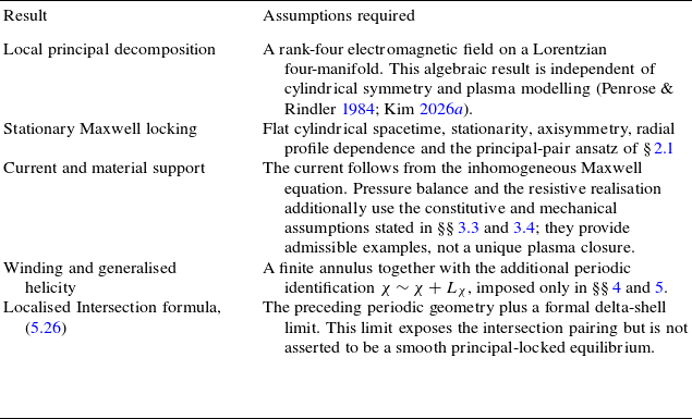

 σ
 σ
 1⩽r/r0⩽2
 σ=0.2
 k1=0.1
 k2=0.2
 Bϕ
 Bχ
 a
 C
 h
 a
 C
 h
 −CB2a′
 −hB2(r2a)′
 p(2)=0

 χ∼χ+Lχ
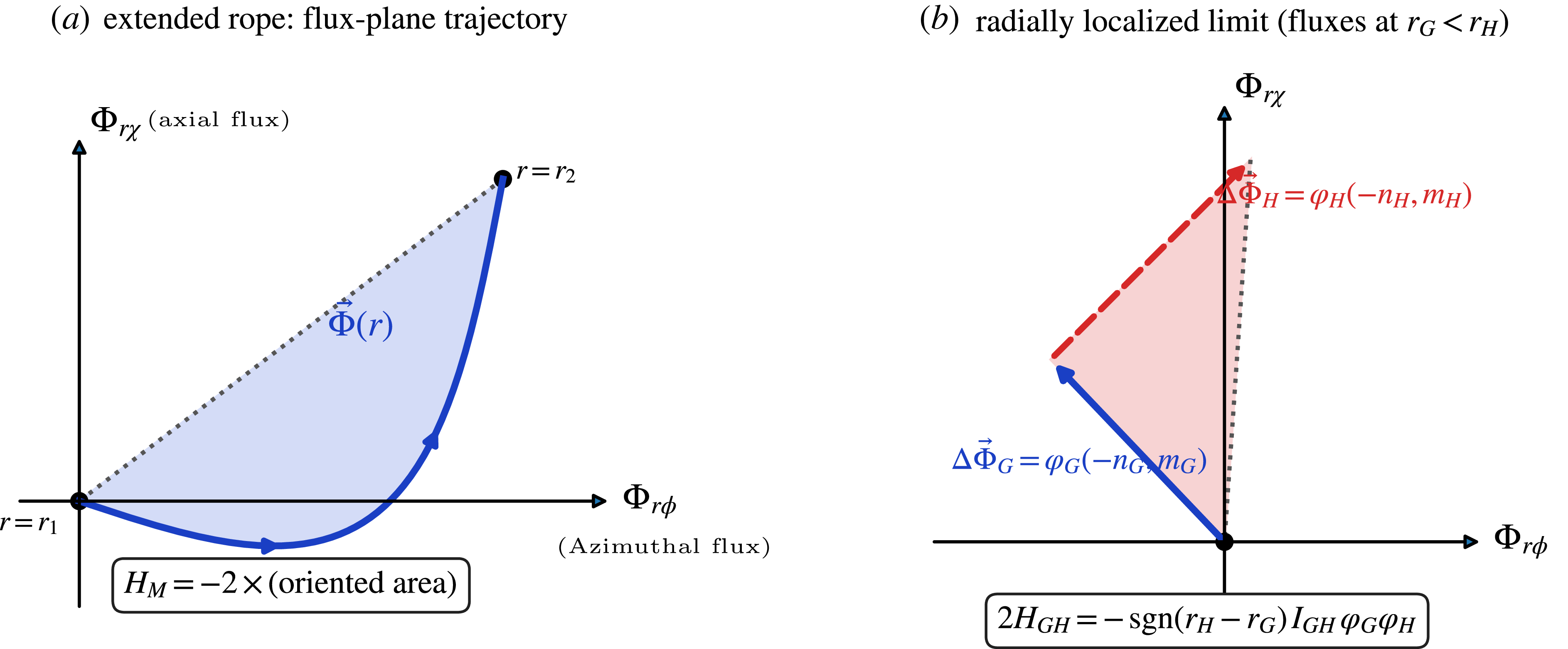
 HM
 Φ(r)
 2HGH=−sgn(rH−rG)IGHφGφH

 Open access

