NOMENCLATURE
- θ
-
pitch angle (deg)
- ω
-
frequency (rad/s)
- φ
-
phase angle (deg)
- M
-
modulus, absolute value of the frequency response
- f
-
specific force (m/s2)
-
(specific force is defined as the external force per unit of mass. The dimensions is (m/s2))
- g
-
gravity (m/s2)
- i
-
input signal
- u
-
output signal (or response)
- Δt
-
measured time difference (s)
- a/c
-
aircraft
- pa
-
aircraft pilot
- ps
-
simulator pilot
- x, y, z
-
along X, Y, and Z axes
Indices
1.0 INTRODUCTION
During the 1970s, the synergistic six-degrees-of-freedom (6DoF) hexapod-type motion system was introduced for flight training simulators. The results of experimental research demonstrated that motion feedback in tracking tasks improved pilot tracking behaviour and tracking performance considerably(Reference Meiry1–Reference Hosman7). The motion cueing of the 6DOF motion systems was well received and became mandatory for Zero Flight Time training. FAA Advisory Circular 120-40 of 1983(8) was the first regulatory document requiring 6DoF motion feedback for Phase II and Phase III flight simulators (Phase II and Phase III were indications of the simulator qualification for pilot training). The motion cueing algorithms for the 6DoF motion systems were based on the publications of Schmidt and Conrad(Reference Schmidt and Conrad9), and Parish, Dieudonne and Martin(Reference Parrish, Dieudonne and Martin10).
However, following the publication of FAA AC 120-40, simulator manufacturers considered the motion cueing of their simulators as an internal part of their product and, as a result, the transparency of the Motion Drive Algorithm (MDA) format and tuning parameters was lost. The adjustment of the MDAs was then – and still is – primarily based on the subjective judgment of experienced pilots. The outcome of this tuning process adjustment is highly dependent on the cooperation between the evaluation pilot and simulator software engineer who assess the final configuration. Being dependent on human experience, there is the potential for variability and errors. Newer versions of the FAA advisory circular 120-40A and 120-40B were published without changing the subjective acceptance of the motion cueing(11,12) . The same held for the ICAO Document 9625 edition 2, 1994(13), the European JAR-STD 1A, 1997(14), and Appendix A to FAA Part 60, 2000(15).
During the 1990s, it became clear that for the training of pilots of commuter aircraft, the Full Flight Simulator (FFS) was relatively expensive in comparison to the use of a FFS for pilot training for large transport aircraft. With the support of the FAA, experimental research to establish the contribution of motion stimulation to the transfer of training was carried out. Quasi-Transfer of Training studies were first performed by Volpe Lab(Reference Bürki-Cohen, Booth, Soja, Disario, Go and Longridge16). Many experimental studies on the contribution of simulator motion based on real or quasi-transfer of training followed. For an overview, see(Reference Winter, Dodou and Mulder17). In this reference, 24 studies on transfer of training are discussed. In the discussion of their study, the authors stated:
In our literature search, strikingly few studies actually measured motion, for example, by means of accelerometers in the simulator cabin. With the exceptions of Bürki-Cohen et al (2004), Martin (1985), and McDaniel, Scott and Browning (1983), none of the flight simulator motion experiments included in our meta-analysis provided an accurate description of the motion hardware and motion drive laws. In fact, in aviation, there are no formal guidelines for simulator motion cueing settings, and the gains and filters of motion platforms are adjusted by trial and error by “motion tuning” experts and pilots.
It is apparent that the researchers who performed the transfer of training studies did not emphasise the important prerequisite of calibrating the tool, i.e. the motion cueing system (the total system transforming the aircraft motions to simulator motions) of the flight simulator used for their experiment. Therefore, one may question the value of the results of these transfer of training studies, i.e. being only valid for the particular simulator used for that specific experimental configuration. Nevertheless, the general suggestion made by the transfer of training studies that the addition of motion feedback does not improve the transfer of training led to the ‘Motion-versus-No-Motion’ discussion. It was also suggested that the removal of the requirement for motion systems would arguably lower the cost of pilot training considerably.
In the spring of 2006, the International Working Group (IWG), under the guidance of the Royal Aeronautical Society, revised ICAO Document 9625 on simulator qualification. In all previous simulator qualification requirements, only the robotic characteristics of the motion system were subject to objective tests. These tests included the bandwidth, latency, leg balance and turnaround bump. Cueing, however, was left to pure ‘function subjective testing’. There was no alternative.
The dynamic characteristics of the motion cueing system are influenced by three components: the MDA, the motion hardware dynamics, and the digital delays in the motion system (computations, digital/analogue conversions, transmissions, etc.). As a result, the authors proposed a more rigorous methodology for these tests(Reference Advani and Hosman18,Reference Advani and Hosman19) in 2006. It involved a frequency-response measurement of the transfer function between the pilot position in the aircraft and in the simulator. In this way, the contribution of the MDA, the motion system dynamics and the time delay due to digital processing could collectively be taken into account.
The aircraft moves through six degrees of freedom, and the simulator uses its own six degrees of freedom to approximate the aircraft motions. Some aircraft motions are directly transformed to the simulator by scaling, while others, such as long-term specific forces, make use of simulator rotations to create the illusion of sustained motions. However, there are also parasitic (undesirable) motions consequential to the filtering or due to system dynamics, and these need to be verified as well. In the OMCT, a total of ten frequency responses are measured – six direct relations for each degree of freedom and four cross-coupling relations.
On request of the authors during a workshop at the AIAA Modelling and Simulation Technologies Conference in 2006, three laboratories performed the proposed test on their research simulators(Reference Advani, Hosman and Potter20). From the results it became clear that a large spread between the dynamic behaviour of motion cueing systems was found. With these foundational results, the simulator industry was convinced that a further development and evaluation of the proposed OMCT could lead to an objective test of the dynamic behaviour of the total motion cueing system in the frequency domain and that a criterion for motion cueing could indeed be developed. In 2011, an evaluation of the final test was started.
In the next sections of this paper, the setup of the Objective Motion Cueing Test, its evaluation and the motion cueing criterion will be discussed.
2.0 MOTION CUEING FUNDAMENTALS
Humans perceive self-motion through the integrated characteristics of their visual, vestibular and proprioceptive systems. Perception of self-motion is important to know where we are, to be able to move around in our environment, and to control our posture. Pilots perceive aircraft motions through the integrated processing of the neural response of the visual and vestibular system due to motion stimulation. The motion feedback in the aircraft improves pilot motion perception and control performance(Reference Hosman7).
In the aircraft, the pilot perceives the aircraft motions with his vestibular system at the pilot position. The perceived specific forces are influenced by the pilot's position relative to the aircraft centre of gravity (cg). In the simulator, the pilot perceives the simulated aircraft motions at the pilot's position in the simulator cab. To transform the aircraft motion resulting from the aircraft model at the aircraft cg, to motion at the pilot position in the aircraft and subsequently to the simulated motions at the pilot position in the simulator, the following steps have to be taken, Fig. 1:
-
1. Calculation of aircraft motion at pilot position in the aircraft, Fpa
-
2. Transformation from aircraft motions at Fpa to simulator upper platform reference frame motions
-
3. Correction of simulator motion to pilot position in the simulator, Fps
-
4. Generation of the simulator motion by the motion system
Transformation of aircraft flight model output to simulator response.

Note that the term ‘motion’ is broadly used. The variables tested are basically specific force and angular acceleration, as the vestibular system is sensitive for these variables
While the aircraft travels over large distances, the simulator motion remains within the boundaries of that system's motion space. This motion space is, in particular for linear translations, about six orders of magnitude smaller than the motion space of transport aircraft operation. The goal of the Motion Drive Algorithm, MDA, is to transform the aircraft motions to simulator motions such that:
-
• The pilot is provided with motion cues to maintain his perception and control behaviour as closely as possible to that in real flight.
-
• The simulator motions remain within the motion space of the motion system, to prevent false cueing if the mechanical limits are reached.
The total transformation of the aircraft motions to simulator motions is primarily influenced by the Motion Drive Algorithm(Reference Schmidt and Conrad9,Reference Parrish, Dieudonne and Martin10,Reference Reid and Nahon21) , but also by the dynamic characteristics of the motion system and by digital time delay of the total transformation process.
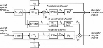
In Fig. 2, the basic scheme of the so-called Classical MDA from(Reference Reid and Nahon21) is presented. The Classical washout scheme consists basically of three channels: the translational channel transforming the input specific force to simulator translations, the rotation channel transforming the input angular rotations to simulator rotations, and the tilt-coordination channel for simulating low-frequency specific force by simulator tilt.
Basic scheme of the classical washout filter(Reference Reid and Nahon21). In this figure β = Euler angle, a = acceleration, Lis = rotation matrix, and Ts = conversion matrix to Euler angle.

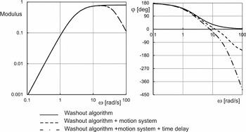
In Fig. 3, an example for the transfer of rotation with the influence of the contributing systems is presented.
Bode plot of the additional influence of the motion system characteristics and digital time delay to the washout algorithm of a high-pass rotation filter.

It is also important to note the influence of the form of the MDA. In order for the simulator to provide a ‘feel’ that is representative for the aircraft, the MDA parameters are typically tuned during acceptance by the evaluation pilot under different simulated flight conditions. Usually, the evaluation pilot's subjective feedback is used to tune these parameters. This, however, does not always lead to a consistently reliable and reproducible tuning of the system.
To improve the motion cueing of full flight simulators and make their characteristics more transparent, a reliable and objective test was required. In 2006, the authors proposed a frequency domain test which could characterise the total dynamic characteristics of the motion cueing system from the pilot cueing perspective(Reference Advani and Hosman18,Reference Advani and Hosman19) . Extensive discussions with the industry led to a number of improvements and, in collaboration with five simulator manufacturers and one university, to a successful evaluation of the test.
3.0 THE OMCT PRINCIPLE
The goal of the OMCT is to objectively measure the frequency responses of the complete motion cueing system at the pilot reference position in the simulator, Fps, and compare this with the motion that would take place at the pilot reference position in the aircraft, Fpa. The motion at Fps is measured while the motion at Fpa is calculated by the equations of motion in the simulation.
In most cases, multiple motion cueing algorithm configurations are used (e.g. in flight or on the ground). The OMCT is separately performed for each of these configurations as applied during training.
The motion cues in the simulator are intended to contribute to the pilot's motion perception in the simulator as they do in the aircraft. For the maximum possible transfer of the rotations and translations from the aircraft environment to the simulator, the modulus of the frequency responses should preferably be unity and the phase should be zero. While this would be the ideal case, the physics of the motion system and the characteristics of the MDA limit these possibilities. Since the simulator cabin moves within the limitations of the motion system, a one-to-one transformation over the whole frequency range is not feasible. Cross-talk between the rotational and translational degrees of freedom of the simulator comes into play due to the form of the algorithms and motion platform dynamics. In some cases, this cross-coupling is desirable (such as gravity align by rotation, which is used to simulate low-frequency specific forces). The net result is that the aircraft motions are transformed to the simulator motions through a complex transfer function.
The OMCT determines the frequency responses for the three rotational and three translational direct input-output relations. In addition, it determines the frequency response of four cross-couplings, i.e. between aircraft pitch and roll inputs to simulator surge and sway responses respectively and, secondly, between aircraft surge and sway inputs to simulator pitch and roll responses respectively. All other input-output relations are of minor importance. In summary, the following frequency responses are determined by the OMCT:
-
1. FSTD pitch response to aircraft pitch input
-
2. FSTD surge acceleration response due to aircraft pitch input.
-
3. FSTD roll response to aircraft roll input
-
4. FSTD sway specific force response due to aircraft roll input
-
5. FSTD yaw response to aircraft yaw input
-
6. FSTD surge specific force response to aircraft surge specific force input
-
7. FSTD pitch attitude response to aircraft surge specific force input
-
8. FSTD sway specific force response to aircraft sway specific force input
-
9. FSTD roll attitude response to aircraft sway specific force input
-
10. FSTD heave specific force response to aircraft heave specific force input
(FSTD is flight simulator training device; see Ref. 13.)
An MDA is composed of high-pass and low-pass filters, transformation matrices, and non-linear blocks such as tilt rate limiting and acceleration limiting(Reference Reid and Nahon21). An MDA may also contain special effects that generate motions not well characterised by the cueing algorithm, such as vibration buffets or short-term accelerations as a function of airport runway bumps. The MDA aims to provide a good balance between cueing of the aircraft motions and the limitation of the simulator motion system.
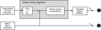
The aim of the OMCT is to determine the basic frequency response characteristics of the total motion cueing system, Fig. 4, while limiting the contribution of the non-linear elements of the motion cueing system as much as possible. The test as described in the RAeS Handbook(22) provides the input frequencies and amplitudes.
Input of the OMCT test signals to the motion cueing system and the measured responses at pilot positions Fpa and Fps.

As long as the motion cueing system may be considered linear, the frequency responses provide a full description of the dynamic behaviour of the motion cueing system in the frequency domain. Therefore, it is important that the range of input frequencies of the test signals cover the normal operating frequency range of the motions that occur during a training exercise. Since during most of the time in operational training the nonlinearities of the motion cueing system are not activated, application of the OMCT provides a reasonable insight into the motion cueing system's characteristics.
The test signals consist of sinusoids at 12 frequencies in the range of 0.1-15.8 rad/s. This frequency range and the number of frequencies have been chosen to achieve an adequate accuracy of the frequency responses over the frequency range of interest.
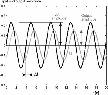
The relationship between the frequency and corresponding modulus M and phase φ defines the system frequency response. For the measurements required, the individual degrees of freedom are excited independently for pitch, roll and yaw, and for surge, sway and heave. For each discrete input frequency defined, the measured relation in modulus and phase should be determined. This can be done manually (by measuring amplitude and phase on the resulting plots like Fig. 5), or by using appropriate digital methods. The modulus M and phase φ are defined as:
 $$\begin{equation}
\begin{array}{l} M(\omega ) = {\rm{amplitude}}\,{\rm{of}}\,{\rm{output}}\,u(\omega )/{\rm{amplitude}}\,{\rm{of}}\,{\rm{input}}\,i(\omega )\\ \varphi (\omega ) = \Delta t\omega 360/2\pi ({\rm{deg}})\quad (\Delta t< 0\,{\rm{for}}\,{\rm{a}}\,{\rm{delay}}) \end{array}
\end{equation}$$
Definition of amplitudes of the input signal i, the output signal u and the time shift Δt.

A careful execution of the test using individual sinusoids takes about three hours. This time can be considerably shortened by applying a sum of sinusoids for the input signals instead of individual signal sweeps. In that case, however, care must be taken in choosing the sample frequency, the sinusoidal frequencies and the total measurement time to obtain an optimal result of the required frequency response based on the use of fast Fourier transform.
From the above description of the OMCT, it is clear that the results describe the motion cueing system dynamic characteristics between Fpa and Fps in the frequency domain. For correct simulation of the aircraft motions at the pilot position in the aircraft (which is the input to the motion cueing system), it is important that the calculation of the specific forces at pilot reference position Fpa is performed correctly.
4.0 THE OMCT EVALUATION
In consultation with the simulator industry, it was decided to evaluate the OMCT in cooperation with the flight simulation industry. This task was led by the authors and carried out through the RAeS Motion Task Team. The industry partners performed the OMCT as described in the RAeS Simulator Qualification Handbook(22), while the authors independently processed the OMCT data, adjusted the test where necessary, proposed a criterion and reported the results to the RAeS and the partners.
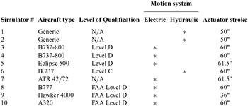
During the evaluation process, five simulator manufacturers (CAE, Moog, L3, Flight Safety International and Rexroth/Opinicus) and also the Delft University of Technology participated in this effort, making the OMCT data from 10 flight simulators available (see Table 1).
Overview of the simulators used in the OMCT evaluation

Note: The certification of simulator #7 was not yet available at the time of the measurements.
Processing of the first OMCT data demonstrated that performing the test for the first time could lead to some errors in the data. Most participants had to go back and correct their measurement techniques or data. The original proposal(Reference Advani and Hosman18,Reference Advani and Hosman19) suggested plotting the OMCT data in a Nichols plot. This was inspired by the presentation of the Sinacori-Schroeder criterion(Reference Sinacori23,Reference Schroeder24) . During the evaluation process, it turned out however that the industry preferred to use the Bode plots to present the OMCT data because that presentation format fitted better with the frequency response data and is common practice in working with cueing characteristics.
For each simulator-MDA combination, the OMCT data were received from the participating organisation. The authors plotted the data in Bode plots and verified the results with each particular participant. In a number of cases this led to further correction of the data.
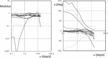
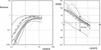
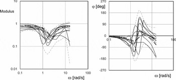
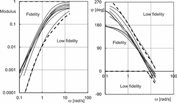
The OMCT data of the 10 simulators was plotted together for each test. The raw data indicated significant variability (see Figs 6, 8 and 9). As a reference, the OMCT data were computed for the results of a motion cueing system optimised for optimum motion feedback (dash-dotted lines in Figs 6, 8 and 9)(Reference Hosman, Advani and Haeck25,Reference Hosman, Advani and Haeck26) .
Frequency response for aircraft pitch rotation to simulator pitch rotation, Test 1. Grey lines indicate the average and ±2 the standard deviation.

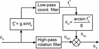
In Test 1, the transfer function of the aircraft pitch angle to simulator pitch angle over the entire frequency range is taken into account (see Fig. 7). Test 1 is configured as such in order to assure that the pitch angle is correctly presented in the simulator during climb and descent, i.e. at low frequencies. The results with the initially received data for the OMCT evaluation are presented in Fig. 6. In the analysis, one simulator showed only high-pass characteristics. As this does not represent aircraft pitch angle at low frequencies, it was considered an outlier and therefore discarded. The source of the error was not indicated to the authors.
Simplified block diagram of the generation of the simulator pitch angle due to aircraft pitch angle.

The next example presents the initial OMCT evaluation data for the transfer of the aircraft yaw to simulator yaw (Fig. 8). There was considerable spread in the results: The maximum and minimum phase angles indicate an average phase difference of about 200 degrees over the whole frequency range. This means that the simulators with the characteristics corresponding with these lines move approximately in opposite direction due to the same aircraft yaw angle changes. This is clearly not correct and the results were discussed with the corresponding participants.
Bode plots for aircraft yaw angle rotation to simulator platform yaw rotation, Test 5.

Based on the characteristics of the Classical MDA(Reference Reid and Nahon27), one would expect the characteristics of a second- and third-order high-pass filter. The majority of the lines indeed correspond with such a filter.
The third example is for Test 6: FSTD surge specific force response to aircraft surge specific force input. Due to the limited maximum displacement in surge of a typical hexapod motion system, as well as the interaction between the high-pass surge filter and the low-pass tilt coordination filter, the frequency responses show large deviations in modulus and phase in the mid-frequency range (Fig. 9). In addition, due to this interaction, the frequency response is sensitive to the non-linear rate limiter in the tilt-coordination channel of the MDA.
Bode plots for aircraft surge input to simulator surge response, Test 6. Grey lines indicate the average and ±2 standard deviation.

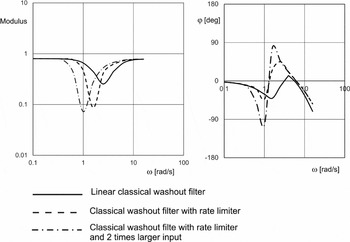
In Fig. 10, the influence of the magnitude of the input signal on the measured frequency response for Test 6 is presented. The frequency responses in Fig. 10 are measured with 12 individual sinusoids as described in Ref. 22 and based on a computer simulation. From this result, it is clear that the accuracy of the frequency responses determined with the OMCT is sensitive to linearity in the MDA. The frequency response accuracy of the Tests 6, 7, 8 and 9 is most sensitive to non-linearity.
The influence of the rate limiter in the translational channel of the MDA on the surge to surge frequency response. Input amplitude with rate limiter 1 and 2 m/s2.

5.0 RESULTS OF THE OMCT EVALUATION
After the final OMCT data of all participants was received, the total data set produced an overview of the state of the art of motion cueing. The feedback by the authors on the OMCT data to the participating organisations during the OMCT evaluation led in most cases to corrections of the data.
In one particular case, the manufacturer completely renewed the adjustment of their MDA. This improvement led to significantly greater acceptance by their test pilots. This manufacturer has since decided to update its entire fleet of devices to reflect these improvements. Other participants are also considering amendments to their MDAs or the tuning sets.
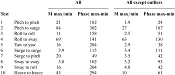
In the final data set of the OMCT evaluation, however, clear outliers remained. In Table 2, an overview is presented of the average width of the modulus and phase variation. It turned out that the results of two of the simulators had to be considered outliers. Ignoring these outliers reduced the width of the modulus and phase variation for the tests 1, 3, 5, 7, 9 and 10 considerably.
The average width of the modulus variation, Mmax/Mmin and the phase variation, φmax - φmin for all tests

The modulus of the frequency responses for the Tests 2 and 4 are small (≤0.05 and 0.18 for Tests 2 and 4, respectively). The frequency responses for Test 6 and 8 are influenced by the non-linearity in the cueing algorithm (Fig. 10).
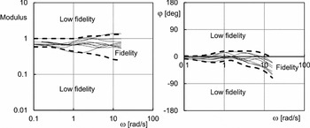
Based on the OMCT data set, after removal of the outliers the boundaries of a motion cueing criterion were established. The results of the final OMCT data set were also compared with the cueing algorithm developed, based on the integrated design of motion cueing systems method as described in Refs Reference Hosman, Advani and Haeck25 and Reference Hosman, Advani and Haeck26 and shown in Figs 6, 8, and 9 by a dash-dotted line. The proposed criterion was discussed with the simulator industry and, after some consideration, accepted for incorporation in Attachment F of ICAO Doc 9625(28). The boundaries of the criterion are presented in the Appendix of this article.
The OMCT (objective motion cueing test) turned out to be a valuable assessment of the motion cueing system. The resulting frequency responses provide a clear view of the dynamic characteristics of the overall motion cueing system. The participating organisations (simulator manufacturers and Delft University) welcomed the test as a valuable methodology for objectively evaluating the total motion performance of flight simulators.
The present boundaries of the criterion are the result of a compromise and, in the opinion of the authors, wider than necessary. More experience with the test has to be gained by the industry before a revision of the boundaries of the criterion may be considered. However, the present criterion rejects in any case all outliers, which is an important improvement compared to the subjective acceptance of motion cueing which did not lead to a consistently reliable and reproducible tuning of motion cueing systems.
In the meantime, DLR Braunschweig, NASA Ames and the NLR Amsterdam have also performed the OMCT with their research simulators(Reference Seehof, Durak and Duda29,Reference Zaal, Schroeder and Chung30) . The FAA has also proposed to incorporate the OMCT in its simulator requirements for FAR 125-Part 60(14).
6.0 DISCUSSION
In this paper, the design and evaluation of the objective motion cueing test for flight simulation training devices is discussed. The simulator industry and the Delft University of Technology participated in this effort into two ways. First, there were interactive discussions with the industry which helped to improve the test and associated definitions. Secondly, the industry and DUT participated actively in the evaluation process by performing the test on their simulators and made the results available for the evaluation.
From the parties involved in these tests, we received positive and encouraging reactions on the results of the OMCT. The frequency responses of the ten tests provide clear insight into the dynamic behaviour of the motion cueing system and enhance the effectiveness of fine-tuning the motion cueing characteristics. The fact that the test and the criterion will be part of the new edition of ICAO Doc 9625(28), and that the FAA has proposed to incorporate the test in FAA Part 60 makes clear that the OMCT is widely accepted.
The original test plan for the OMCT is described in Section 3e(1) of the RAeS Flight Simulation Evaluation Handbook(Reference Reid and Nahon21). Based on the experience gained with the OMCT during the evaluation described herein, a revised test plan has been developed and proposed to replace Section 3e(1) in the next edition of this handbook(Reference Hosman and Advani31). The most important changes are related to a more detailed description of the tests, the appointment of the dimension of the frequency responses of Tests 2, 4, 7, and 9, and the addition of the criterion boundaries.
The execution of the test as described takes approximately three hours and may be shortened significantly by using a sum of sinusoids as input test signals. This requires careful selection of the sinusoid frequencies, the sample frequency and the duration of the test signal, as defined by the theory of the fast Fourier transformations. The final accuracy of the frequency responses depends on the measurement noise. Accurate testing to evaluate the advantages and disadvantages of this method is required in order to develop adequate procedures for the full application of the method.
7.0 CONCLUSIONS
OMCT data and a motion cueing criterion are now available for transport aircraft simulation for the in-flight condition. With this, a first important step in the improvement of flight simulator motion cueing has been achieved. Additional measurements and evaluation are required to develop a criterion for the on-ground condition of transport aircraft simulation.
The same applies to helicopter simulation, where different motion cueing algorithm settings are used for hover and forward flight.
Finally, there are a number of research simulators equipped with motion systems which deviate from the typical hexapod motion systems on training simulators, including the NASA Ames Vertical Motion Simulator (US), Desdemona (Netherlands), and the Wright-Patterson Air Force Base LAMARS Simulator. OMCT data for the individual degrees of freedom and typical cross- relations of those simulators can help to compare the capabilities of these research simulators and be very helpful in the selection of the motion system design of future research devices.
Appendix
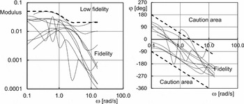
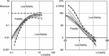
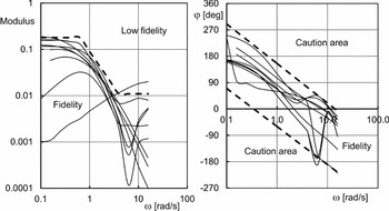
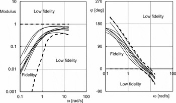
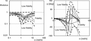
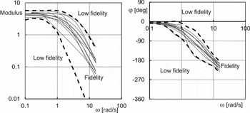
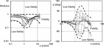
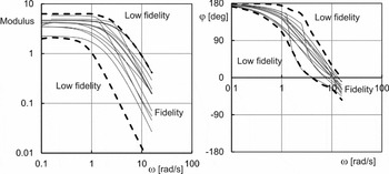
In the figures below, the criteria boundaries for all ten OMCT tests are presented together with the OMCT data received from the participating organisations in the OMCT evaluation. The criteria boundaries are indicated with dotted lines.
The boundaries for the modulus and phase of the frequency response for Test 1.

The boundaries for the modulus (m/deg) and the caution area for the phase of the frequency response for Test 2.

The boundaries for the modulus and phase of the frequency response for Test 3.

The boundaries for the modulus (m/deg) and the caution area for the phase of the frequency response for Test 4.

The boundaries for the modulus and phase of the frequency response for Test 5.

The boundaries for the modulus and phase of the frequency response for Test 6.

The boundaries for the modulus in (deg/(m/s2)) and phase of the frequency response for Test 7.

The boundaries for the modulus and phase of the frequency response for Test 8.

The boundaries for the modulus in (deg/m/s2)) and phase of the frequency response for Test 9.

The boundaries for the modulus and phase of the frequency response for Test 10.