



1. Introduction
An important criterion used to describe the dynamics of populations is exhibited in [Reference Cohen, Plank and Law10], among others, via the expression known as Taylor’s law (TL). This originated as an empirical pattern in ecology in such a way that, on comparable populations, the variance of each sample was approximately proportional to a power of the mean of that sample. Thousands of papers have been dedicated to the study of TL. This limits our ability to provide a comprehensive review. An important survey on the topic is [Reference Eisler, Bartos and Kertész21]. A key motivation for our work can be found in [Reference Kendal and JØrgensen23], which provides a central-limit-like convergence that explains TL, or [Reference Brown, Cohen and De la Pena7], which introduces a self-normalized empirical version of TL for some distributions with infinite mean.
The question posed here is about what happens if we observe only one trajectory of a random phenomenon. We clearly need ergodicity conditions to consistently investigate the expressions related to TL. Therein, we prove a novel theory for TL under dependence in the case when only a trajectory of the process of interest
 $(X_t)_{t\in\mathbb{Z}}$
is observed. It can, of course, be accommodated in the context of independent copies of the process
 $(X_t)_{t\in \mathbb{Z}}$
observed over different samples. For example, this is the case when dealing with mortality time series over ages or even regions [Reference Bohk, Rau and Cohen6], which means that the dependence in the sample has already been considered. In order to obtain laws of large numbers and the possibility of fitting those expressions, we restrict our paper to a specific frame. Essentially, we consider ergodic behaviors and focus on stationary time series. In this case, we are in a position to define a general TL possibly taking into account the dynamic behavior of the process of interest and not only its marginal distribution.
To achieve this, we proceed in two steps. First, we strictly extend the TL to the ergodic (dependent) setting, which we will call a static TL since it only relies on the marginal distribution of the stationary process
 $(X_t)_{t\in \mathbb{Z}}$
. Second, we introduce an alternative dynamic TL. The main contribution of the paper is to introduce such a TL that not only involves the marginal distribution of
 $X_0$
but also relies on the second-order structure of the process
 $(X_t)_{t\in \mathbb{Z}}$
, thus accounting for the dependence of the blocks. Recall, for example, that the sample average and variance are accurate measures of the mean and variation in the population, which gives sense to TL along some trajectory. However, the timeliness of our approach is supported by the findings of [Reference Reuman, Zhao, Sheppard, Reid and Cohen25], where it is shown that changes in synchrony (which may be caused by climate change) modify and can invalidate the TL. By incorporating the entire history of the time series, our dynamic approach to TL mitigates the effect of these changes.
The current work is developed in the context of weakly dependent variables that include, for example, Bernoulli shifts of independent and identically distributed (i.i.d.) random variables, such as
 $X_t = F\big(X_{t-1},X_{t-2}, \ldots;\, \xi_t\big)$
[Reference Doukhan and Wintenberger17], which depends on the complete past history of the process and some innovations; the simplest example is the case of ergodic Markov chains
 $X_t= F (X_{t-1} ; \xi_t )$
but this new approach also extends to more complex situations, such as infinite moving averages of i.i.d. inputs
 $X_t=\sum_{j=0}^{\infty}a_j X_{t-j}+\xi_t$
. Larger classes of examples, including ARCH, GARCH-type models, integer-valued GLM models, and possibly integer-valued models, may be found in [Reference Dedecker, Doukhan, Lang, Leon, Louhichi and Prieur12] and [Reference Doukhan13]; for more models see also [Reference Doukhan and Neumann16], [Reference Doukhan, Fokianos and Rynkiewicz18], and [Reference Fokianos, Stove, Tjostheim and Doukhan22], for example. Note that those classes of models and many others may easily fit the conditions in the current results, giving context to our settings and results. Such models include dependence over time and should be used in order to describe the dynamical evolution of a population [Reference Cohen, Plank and Law10]. It is, in fact, relevant to population dynamics and in particular to ecological applications; see also [Reference Cohen and Saitoh8], [Reference Saitoh29], and the references therein.
The static TL is a proper characteristic of marginal distributions. Since this novel approach includes consideration of dynamical issues, it is a better application of a TL that depends on the whole distribution of the analyzed process. In [Reference Cohen, Plank and Law10], the question of checking the validity for TL for some random phenomenon is addressed in the setting of i.i.d. sequences. Formally, for an integer
 $k>1$
and a sequence of positive random variables, the relation
 $\text{Var}Y=c (\mathbb{E} Y)^\alpha$
with
 $c\in \mathbb{R}$
and
 $\alpha>0$
was shown to hold in many empirical applications. This means that the consistency of empirical counterparts for those expressions is proved for the convergence in mean in the expressions
 \begin{equation*}c\approx \dfrac{\widehat{\text{Var}Y}}{\big(\widehat{\mathbb{E} Y}\big)^\beta}, \quad \text{with}\quad \widehat{\mathbb{E} Y}=\overline Y\ =\ \dfrac 1k\sum_{i=1}^kY_i\quad \text{and}\quad \widehat{\text{Var}Y}= \dfrac 1{k-1}\sum_{i=1}^k\big(Y_i-\overline Y\big)^2.\end{equation*}
Here, the expressions of the variance
 $\text{Var}Y$
and
 $\mathbb{E} Y $
make sense since those parameters provide a first approximation to the distributions of i.i.d. samples. Another analogous expression emerges in actuarial and financial sciences related to the so-called measures of variation, e.g. [Reference Albrecher and Teugels1,Reference Albrecher, Ladoucette and Teugels2]. It is strongly related to the ratio
 \begin{equation*}d\approx \dfrac{\widehat{\mathbb{E} Y^2}}{\big(\widehat{\mathbb{E} Y}\big)^\beta}, \quad \text{with}\quad \widehat{\mathbb{E} Y^2}=\dfrac 1k\sum_{i=1}^kY_i^2.\end{equation*}
In [Reference Albrecher, Ladoucette and Teugels2], the convergence of such self-normalized sums is investigated in detail. For instance, it is proved that the convergence in distribution of suitably normalized ratios holds for heavy- or light-tailed distributions. In [Reference Albrecher and Teugels1], the above approximation is proved to hold in
 $\mathbb{L}^p$
via the limit expression for each of the moments of the above ratio. In [Reference Cohen, Davis and Samorodnitsky9], the relevant case of heavy-tailed models is investigated, including vector-valued self-normalized results as well as empirical TL under heavy-tailed assumptions. Unlike these examples, our paper is principally concerned with dependent random variables, which have received less attention in the literature. Indeed, the theoretical literature has, thus far, dealt with the independent case, also referred to as the classic TL. We restrict our work to random variables with moments of order greater than 4. However, we deal with dependent random variables and thus handle the case of time series.
To the best of our knowledge, the current paper is the first attempt to include the dependence structure in such TLs. To achieve this, we first consider stationary and ergodic processes
 $(X_i)_{i\in\mathbb{Z}}$
to decompose the sequence of interest into Bernstein blocks. This allows us to divide the data up into blocks in such a way as to adequately control the dependence between blocks. For instance, the setting considered in [Reference Cohen, Davis and Samorodnitsky9] does not require the use of the Bernstein block variant of TL we consider in this paper. Indeed, this technique will be crucial to investigating the asymptotic distribution of the considered quantities in order to derive statistical properties for the two different TLs (static and dynamic). Formally, we show that the above expressions admit convergent behaviors. This follows the same idea as for the ‘classic’ behavior of such laws. Indeed, the variance involved in the above-mentioned expressions has a counterpart in the weakly dependent cases. Specifically, as explained in [Reference Doukhan13], [Reference Doukhan and Louhichi15], [Reference Rio26], and [Reference Doukhan14] under an adapted weak dependence assumption, the partial centered sums renormalized with a
 $\sqrt n-$
factor converge to a centered Gaussian distribution with variance
 $\sigma^2$
, such that
 \begin{equation}\sigma^2 = \sum_{j=-\infty}^\infty \text{Cov}\big(X_0,X_j\big).\end{equation}
Accordingly, the extension of the TL will inevitably incorporate the series of covariances, and not just over marginal distributions. By doing so, we take the view that such an index has a different meaning to the usual TL, which only depends on marginal distributions. However, this topic exceeds the scope of the paper. Instead, we will develop the limiting behavior of the statistics in question. The results developed throughout the paper take into account this new dynamic exponent as well as the classical (static) Taylor’s exponent; both are considered for general classes of dependent random processes.
The paper is organized as follows. In Section 2 we introduce the empirical expressions necessary to deal with both the dynamic and static TLs in a dependent setting. In Section 3 we deal with limit theory under these laws. (To this end we describe a Bernstein block technique used throughout the paper in order to control the dependence. Hence the limit distribution of suitably normalized expressions for both static and dynamic indices is proved in Section 3.) Finally, Section 4 is dedicated to a test of goodness-of-fit for the dynamic TL to hold. This means that the two results together will ensure a test for both TLs to hold. The necessary dependence tools and technical results are introduced in the appendices.
2. Self-normalized sums
Let
 $(Y_i)_{i\in\mathbb{Z}}$
and
 $(X_i)_{i\in\mathbb{Z}}$
be two sequences of non-negative and identically distributed random variables. Since this paper is focused on dependent and dynamic samples, we will henceforth let
 $(Y_i)_{i\in\mathbb{Z}}$
denote the statistics under consideration and let the sequence
 $(X_i)_{i\in\mathbb{Z}}$
denote the classic TL. Before we introduce TL with the general exponent
 $\beta>0$
, we recall the statistics associated with the usual TLs for
 $\beta=2$
, and we then turn to the dependent case.
Formally, with
 $k>0$
, we define
 $S_k$
as the ratio
 \begin{equation*}S_k = \dfrac{\sum_{j=1}^kY_j^2/k}{\Big(\sum_{j=1}^kY_j/k\Big)^2}=k\cdot \dfrac{\sum_{j=1}^kY_j^2}{\Big(\sum_{j=1}^kY_j\Big)^2}.\end{equation*}
Hence, with
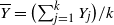 $\overline Y=\Big(\sum_{j=1}^kY_j\Big)/k$
, we can write
 \begin{equation}S_k=\dfrac{\sum_{j=1}^kY_j^2/k}{\overline Y^2}=\dfrac{k-1}k\cdot T_k+1,\end{equation}
where we let
 $T_k$
denote the TL statistics defined as
 \begin{equation}T_k = \dfrac{\sum_{j=1}^k\bigl(Y_j-\overline Y\bigr)^2/({k-1})}{\overline Y^2}.\end{equation}
This is a plug-in estimate of
 $T={\sigma^2}/{m^2}$
, with
 $m=\mathbb{E} Y_1$
and
 $\sigma^2=\text{Var}Y_1$
. Note that we can write
 \begin{equation}T_k = \dfrac{k}{k-1}\cdot (S_k-1),\end{equation}
so that the result of the asymptotic behavior of
 $T_k$
may be plugged into those for
 $S_k$
. The above relation provides us with a link between results for the self-normalized statistics
 $S_k$
and for Taylor’s statistics
 $T_k$
. More generally, for
 $\beta >0$
, as in [Reference Cohen, Plank and Law10], we consider TL with order
 $\beta$
for
 $\sigma^2=cm^\beta$
, where the corresponding statistics can be written as
 \begin{equation*}T_{k,\beta} = \dfrac{\sum_{j=1}^k\bigl(Y_j-\overline Y\bigr)^2/({k-1})}{\overline Y^\beta}.\end{equation*}
In this case, set
 $W_k=\sum_{j=1}^k\bigl(Y_j-\overline Y\bigr)^2/({k-1})$
; then
 \begin{align*} S_{k,\beta} &=\dfrac{\sum_{j=1}^kY_j^2/k}{\overline Y^\beta}\\ &= \dfrac{k-1}k\cdot T_{k,\beta}+\overline Y^{2-\beta}\\&=\dfrac{k-1}k\cdot \dfrac{ \sum_{j=1}^k\bigl(Y_j-\overline Y\bigr)^2/({k-1})}{\overline Y^{\beta}}+\overline Y^{2-\beta}\\ &= \biggl(\dfrac{k-1}k\cdot T_{k}+1\biggr)\overline Y^{2-\beta}.\end{align*}
In the dependent framework of a stationary time series, we use Bernstein blocks [Reference Bernstein5] to divide the sample
 $X_1,\ldots, X_n$
, for
 $n>0$
, into blocks of a given size to control the dependence between the blocks. To this end, we consider an integer
 $p_n\in\{1,\ldots,n\}$
and let
 $k_n=[n/p_n]$
. We then let
 $Y_i^{(n)}$
denote the sequence of partial sums over observations in block
 $B_{i,n}$
, that is,
 \begin{equation}Y_i^{(n)} = \dfrac1{p_n}\sum_{j\in B_{i,n}}X_j, \quad B_{i,n} = \big[(i-1)p_n+1,ip_n\big]\bigcap \mathbb{N} , \quad 1\le i \le k_n.\end{equation}
Hence the statistics under consideration defined in (2.2) and (2.1) with
 $k=k_n$
can now be denoted respectively as
 $S^{(n)}_\beta$
and
 $ T_\beta^{(n)}$
:
 \begin{align*}{ \overline Y}^{(n)}&= {\dfrac1{k_n}\sum_{i=1}^{k_n} Y_i^{(n)}},\\
S_\beta^{(n)}&= \dfrac{\sum_{j=1}^{k_n}\Big(Y^{(n)}_j\Big)^2/k_n}{\Big(\overline Y^{(n)}\Big)^\beta},\\
T_{\beta}^{(n)}&= \dfrac{\sum_{j=1}^{k_n}\Big(Y^{(n)}_j-\overline Y^{(n)}\Big)^2/({k_n-1})}{\Big(\overline Y^{(n)}\Big)^\beta}.\end{align*}
Moreover, for the sake of homogeneity, we instead let
 $S^{(n)}$
denote the expression
 $S_2^{(n)}$
.
Remark 2.1. (Bernstein blocks.) First, the reader is referred to Appendix A.2 for a second-order analysis of the behavior of partial sum processes in (2.4), and Appendix A.3 for a higher-order analysis.
Second, we note that, with additional blocks with sizes less than
 $p_n$
, we can use the entire data set, i.e.
 $X_1,\ldots,X_n $
, by setting
 $ B_{k_n+1,n}=[k_np_n+1, n]$
. By doing so, we do not affect the behavior of partial sums when
 $k_n\to \infty$
. Indeed, if the condition
 $a>1$
is fulfilled in (A.3) (see Appendix A.2), we can show that
 \begin{equation*}\text{Var}\Biggl(\sum_{j\in B_{k_n+1,n}}X_j\Biggr)={\text{O}} (p_n)\ll n,\end{equation*}
which entails that partial sums, up to n, behave the same way as sums over all blocks with size
 $p_n$
, as soon as
 $\sigma^2\ne0$
. In fact, in this case we shall have
 \begin{equation*}\lim_{p\uparrow\infty}\text{Var}\Biggl(\sum_{i=1}^pX_i/\sqrt{p}\Biggr)= \sigma^2 .\end{equation*}
Therefore, for the sake of readability, we do not consider this correction term henceforth.
Remark 2.2. (Dynamic TL with exponent
 $\beta$
.) For
 $\beta >0$
, we extend the above expressions for dynamic TL with order
 $\beta$
. Recall that in this case we are expecting a relationship of the form
 $\sigma^2=cm^\beta$
. In fact,
 $ T^{(n)}$
is associated with TL with exponent
 $\beta=2$
, and the following simple algebraic relation allows consideration of all the possible exponents
 $\beta$
. Notably,
 \begin{equation}S_{\beta}^{(n)}=\dfrac{\sum_{j=1}^{k_n}\Big(Y_j^{(n)}\Big)^2/k_n}{\Big(\overline Y^{(n)}\Big)^\beta}= \biggl(\dfrac{k_n-1}{k_n}\cdot T^{(n)}+1\biggr)\Big(\overline Y^{(n)}\Big)^{2-\beta},\end{equation}
which allows us to consider the TLs for more general settings.
3. Limit theory in distribution
Note that in this dependent framework,
 $\overline Y\equiv \overline X^{(n)}=(X_1+\cdots+X_n)/n$
is simply the empirical mean of the observed process
 $(X_i)_{i\in \mathbb{Z}}$
. Under basic ergodic assumptions, we have
 \begin{equation*}\lim_n \overline X^{(n)}=\mathbb{E} X=m\quad \text{a.s.}\end{equation*}
Hence the asymptotic behavior of the expression
 $T^{(n)}$
corresponding to
 $T_k$
in (2.3) for this dependent setting is
 \begin{equation*} \bar T^{(n)} = \dfrac1{m^2}\cdot\dfrac1{k_n}\sum_{i=1}^{k_n}\Big(Y_i^{(n)}-\overline X^{(n)}\Big)^2,\end{equation*}
which means that
 $\lim_n T^{(n)}/\bar T^{(n)}=1$
. Henceforth, we let
 \begin{equation*} \tilde T^{(n)} = \dfrac1{m^2}\cdot\dfrac1{k_n}\sum_{i=1}^{k_n}\Big(Y_i^{(n)}-m\Big)^2.\end{equation*}
Using assumption (1.1), for
 $\lim_np_n=\infty$
, standard conditions imply that
 \begin{equation}G_{i,n}=\sqrt{p_n}\Big(Y_i^{(n)}-m\Big) \quad \text{for all } 1\le i\le k_n,\end{equation}
has a
 ${\mathcal N}\big(0,\sigma^2\big)$
-standard Gaussian asymptotic behavior for each
 $ i\ge 1$
. Moreover, we have
 \begin{equation}\lim_n\mathbb{E} \big(G_{i,n}\big)^2=\sigma^2 \quad \text{for all } i\ge 1.\end{equation}
Remark 3.1. We remark that the classic (or static) TL corresponds to
 $p_n=1$
. In this case the corresponding blocks are no more asymptotically Gaussian, and thus the above asymptotic Gaussian behavior does not hold. Thus a separate discussion will be needed.
The relation (3.2) entails that we need to explicitly center the expression for
 $G_{i,n}^2$
. Thus, with the notation (3.1) we define the centered sequence
 \begin{equation}U_{i,n} = G_{i,n}^2-\mathbb{E} G_{i,n}^2 \quad \text{for all } 1\le i\le k_n,\end{equation}
or, more specifically,
 \begin{align*}\notag\tilde T^{(n)}&= \dfrac1{nm^2}\sum_{i=1}^{k_n}U_{i,n}+\dfrac1{nm^2}\sum_{i=1}^{k_n}\mathbb{E} G_{i,n}^2 \\ &= \dfrac1{nm^2}\sum_{i=1}^{k_n}U_{i,n}+\dfrac1{p_nm^2}\sigma^2+\dfrac{E G_{i,n}^2-\sigma^2}{p_nm^2}.\end{align*}
We now use the bound (A.5) to derive
 $\mathbb{E} G_{i,n}^2-\sigma^2={\text{O}}(1/{p_n})$
. To this end, by setting
 \begin{equation}{\mathcal G}_{n}=\dfrac1{m^2\sqrt{k_n}}\sum_{i=1}^{k_n} U_{i,n},\end{equation}
we deduce that
 \begin{equation*}g^{(n)} \equiv \sqrt{k_n}\biggl(p_n\tilde T^{(n)}- \dfrac{\sigma^2}{m^2}\biggr) ={\mathcal G}_{n}+{\text{O}} \biggl(\dfrac {\sqrt{k_n}}{p_n}\biggr),\end{equation*}
or equivalently
 \begin{equation*}g^{(n)} = {\mathcal G}_{n}+{\text{O}} \biggl(\sqrt{\dfrac {n}{p_n^3}}\biggr),\end{equation*}
since
 $n=k_np_n$
.
Next, we will prove in Theorem 3.1 that
 ${\mathcal G}_{n}$
admits a Gaussian asymptotic behavior
 ${\mathcal N}\big(0,\Sigma^2\big)$
by using Lemma 3 of [Reference Bardet, Doukhan, Lang and Ragache4]. We will refer to Appendix A.4 to derive the necessary dependence conditions. To this end, assume that for some
 $r>4$
,
 $\mathbb{E}|X_0|^r<\infty$
; then Lemma A.1 (see also [Reference Dedecker, Doukhan, Lang, Leon, Louhichi and Prieur12, equation (4.2.6)]) implies that
 $\big|\text{Cov} \big(U_{0,n},U_{q,n}\big)\big|\le C\big(\theta_n^U(q)\big)^{\frac{r-2}{r-1}} $
from weak dependence conditions for
 $q\ne0$
. Moreover, conditions for moments of
 $G_{i,n}$
with order
 $\delta >2 $
to be bounded are given in Lemma A.1. Now, in order to derive Lemma 3.1, we note that Lemmas A.2 and A.3 provide the conditions to ensure the existence of some
 $r>4$
such that
 $\|X_0\|_r<\infty $
. In fact, one needs conditions (A.8) or (A.9) to hold, as well as the following limit behaviors:
 \begin{equation*}\lim_{n\to \infty} p_n^2\sum_{\ell=1}^\infty \alpha^{\frac{r-4}{r}}(p_n\ell )=0\quad \text{and}\quad \lim_{n\to \infty} p_n^2\sum_{\ell=1}^\infty \theta^{\frac{r-4}{r-2}}(p_n\ell )=0.\end{equation*}
Under such conditions, we can state the following lemma.
Lemma 3.1. Assume that
 $\|X_0\|_r<\infty $
for some
 $r>4$
, and either
 $\alpha(q)={\text{O}} \big(q^{-\alpha}\big)$
or
 $\theta(q)={\text{O}} \big(q^{-\theta}\big)$
holds for
 $ \alpha>2\cdot {r}/{(r-4)}$
, or
 $ \theta>2\cdot {(r-2)}/{(r-4)}$
. Then we have
 \begin{equation*}\lim_{n\to\infty}\sum_{\ell\ne0} \big|\text{Cov}\big(U_{0,n},U_{\ell,n}\big)\big|=0.\end{equation*}
Also, we have
 \begin{equation*}\notag\Sigma^2=\dfrac1{m^4}\lim_n\mathbb{E}\big( U_{0,n}\big)^2.\end{equation*}
Proof.Letting
 $\widetilde X_i=X_i-m$
for
 $i\ge1$
, we can write
 \begin{align}\Sigma^2&=\dfrac1{m^4}\lim_n \dfrac 1{k_n}\text{Var}\Bigg(\sum_{i=1}^{k_n} U_{i,n}\Bigg) \notag \\
& =\dfrac1{m^4}\lim_n\mathbb{E}\big( U_{0,n}\big)^2 \notag \\
&=\dfrac1{m^4}\lim_n\text{Var}G^2_{0,n} \notag \\
&=\dfrac1{m^4}\lim_n\dfrac 1{p_n^2}\sum_{i,j,i^{\prime},j^{\prime}=1}^{p_n}\text{Cov} \Big( \widetilde X_i\widetilde X_{i^{\prime}}, \widetilde X_{j}\widetilde X_{j^{\prime}}\Big) \notag \\
&=\dfrac1{m^4}\sum_{i,j^{\prime}=1}^{p_n}\text{Cov} \Big(\widetilde X_0 \widetilde X_i, \widetilde X_0\widetilde X_{j}\Big).\end{align}
Remark 3.2. (Cumulants.) Note that (3.5) is related to the cumulants
 $\kappa\big(X_0,X_u,X_v,X_w\big)$
. Recall that
 $\kappa(X,Y,Z,T)$
is the coefficient of
 $t_1t_2t_3t_4$
in the Taylor expansion of
 $\log \mathbb{E} \exp({\text{i}} t\cdot {\mathbf V}) $
, if
 $t=(t_1,t_2,t_3,t_4)$
and
 ${\mathbf V}=(X,Y,Z,T)$
. If the process is Gaussian, then the cumulants of order greater than 2 all vanish. In any case, using [Reference Leonov and Shiryaev24] (see also [Reference Rosenblatt28] or [Reference Bardet, Doukhan and Lang3]), we can show that if all the moments are well-defined, then
 \begin{equation*}\text{Cov} ( XY, ZT)=\kappa(X,Y,Z,T)+\text{Cov}( X,Z)\text{Cov}( Y,T)+\text{Cov}( X,T)\text{Cov}( X,Z),\end{equation*}
since
 \begin{align*} \kappa(X,Y,Z,T)&= \text{Cov}( XY, ZT)-\text{Cov}( X,Y)\text{Cov}( Z,T)\\ &\quad -\text{Cov}( X,Z)\text{Cov}( Y,T)-\text{Cov}( X,T)\text{Cov}( X,Z).\end{align*}
Thus Remark 3.2 implies that
 \begin{align*} \text{Cov}\!\left( X_i X_{i^{\prime}}, X_{j}\!X_{j^{\prime}}\right)& = \kappa\!\left(X_i, X_{i^{\prime}}, X_{j}, X_{j^{\prime}}\right) + \text{Cov}\!\left( X_i, X_{j}\right)\text{Cov}!\left( X_{i^{\prime}}X_{j^{\prime}}\right) \\
&\quad + \text{Cov}\!\left( X_i ,X_{j^{\prime}}\right)\text{Cov}!\left( X_{i^{\prime}},X_{j}\right).\end{align*}
It thus follows that we may write
 $m^4\Sigma^2=\lim_nA_n$
with
 \begin{align*}A_n&= \dfrac1{p_n^2} \sum_{i,j,i^{\prime},j^{\prime}=1}^{p_n}\text{Cov}\!\left( X_iX_{i^{\prime}}, X_{j}X_{j^{\prime}}\right)=2 B_n+C_n,\\
B_n&= \dfrac1{p_n^2} \sum_{i,j,i^{\prime},j^{\prime}=1}^{p_n}\text{Cov}\!\left( X_i, X_{j}\right)\text{Cov}!\left( X_{i^{\prime}}X_{j^{\prime}}\right),\\
C_n&= \dfrac1{p_n^2} \sum_{i,j,i^{\prime},j^{\prime}=1}^{p_n}\kappa !\left( X_i, X_{j},X_{i^{\prime}}X_{j^{\prime}}\right).\end{align*}
Hence it is easy to prove that
 $ \lim_n B_n =\sigma^4$
and
 $ \lim_n C_n =0$
when the cumulant sums condition (3.6) holds. This assumption can be written as
 \begin{equation}\sum_{i,=1}^{\infty} \sum_{j=1}^{\infty} \sum_{k=1}^{\infty}\ |\kappa (i,j,k)|<\infty, \quad \text{with } \kappa (i,j,k)=\kappa \big(X_0, X_{i},X_{j}X_{k}\big).\end{equation}
We have thus proved, using Lemma 3.1, that if (3.6) holds, then Proposition 3.1 allows us to specify the limit variance
 $\Sigma$
in the central limit theorem (CLT).
Remark 3.3. (Sufficient conditions.) Condition (3.6) is widely discussed in [Reference Rosenblatt27] and Theorem 4 on page 138 provides a sufficient condition for (3.6) to hold; see also [Reference Rosenblatt28]. This condition is also used as condition M in [Reference Bardet, Doukhan and Lang3], in which a precise study provides the reader with sufficient strong mixing conditions which are under
 $\theta$
-weak dependence. More precisely, if
 $\mathbb{E}|X_0|^r<\infty$
, then condition (3.6) holds if one of the following additional conditions holds:
 \begin{equation*}\sum_{j=1}^\infty j^{\frac 2{r-4}}\alpha(j)<\infty\quad \text{and}\quad \sum_{j=1}^\infty \theta^{\frac{r-4}{r-1}}(j)<\infty.\end{equation*}
We should note that these conditions are not necessary for (3.6) but they are implied by the assumptions in Theorem 3.1.
Proposition 3.1. Assume that conditions in Lemma 3.1 and (3.6) hold; then
 \begin{equation}\Sigma^2=2\cdot\dfrac{\sigma^4}{m^4}.\end{equation}
Now assume that
 $\lim_{n\to\infty} {n}/{p_n^3}=0$
, and simply let
 \begin{equation} p_n=[\kappa n^{\zeta}] \quad \text{with } \zeta>\dfrac13.\end{equation}
Then we will prove that
 \begin{equation}\sqrt{k_n}\bar T^{(n)}={\mathcal G}_n+\sqrt{{{k_n}}}\cdot\dfrac{\sigma^2}{m^2}+\sqrt{k_n}\big(\bar T^{(n)}-\tilde T^{(n)}\big)+{\text{O}} \biggl(\sqrt{\dfrac {n}{p_n^3}}\biggr).\end{equation}
For this, we remark that the first term comes from the ergodic theorem and the CLT for empirical means. For the additional term, the centered Taylor’s statistics may be decomposed as follows:
 \begin{equation*}\bar T^{(n)}-\tilde T^{(n)}=\dfrac1{m^2}\Big(\overline X^{(n)}-m\Big)\Biggl(\dfrac1{k_n}\sum_{i=1}^{k_n}\Big(Y_i^{(n)}-m\Big)+\Big(\overline X^{(n)}-m\Big)\Biggr).\end{equation*}
The bound
 $\overline X^{(n)}-m= {\text{O}} (1/\sqrt{n})$
holds from (A.2). Similarly, we have
 $\text{Var}\Big(Y_i^{(n)}-m\Big)= {\text{O}} (1/{p_n})$
, and if (A.3) holds for
 $a>2$
, then
 \begin{equation*}\text{Var}\Biggl(\sum_{i=1}^{k_n}(Y_i^{(n)}-m)\Biggr)={\text{O}} \big(k_n/{p_n}\big).\end{equation*}
Indeed, we can see that
 \begin{align}\notag\text{Var}\Biggl(\sum_{i=1}^{k_n}Y_i^{(n)} \Biggr)&= \sum_{|\ell| \lt k_n}(k_n-|\ell|)\text{Cov}\Big(Y_0^{(n)},Y_\ell^{(n)}\Big) \\
&\le {\text{O}}\biggl(\dfrac{k_n}{p_n}\biggr)+2k_n\sum_{\ell=1}^{k_n}\Big|\text{Cov}\Big(Y_0^{(n)},Y_\ell^{(n)}\Big)\Big|.\end{align}
Thus
 \begin{equation} \text{Var}\Biggl(\sum_{i=1}^{k_n}Y_i^{(n)}\Biggr)={\text{O}} \biggl(\dfrac{k_n}{p_n}\biggr).\end{equation}
However, this is not straightforward as it needs a thorough investigation of the second term on the left-hand side of (3.10). In fact, for some
 $q\equiv q_n<p_n$
, which will be specified below, in order to prove this we need to decompose
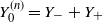 $Y_0^{(n)}=Y_-+Y_+$
such that
 \begin{equation*}Y_-=\dfrac1{p_n}\sum_{i=1}^{p_n-q_n}X_i, \quad Y_+=\dfrac1{p_n}\sum_{i=p_n-q_n+1}^{p_n}X_i .\end{equation*}
Then, with
 $\tilde k_n=[n/(p_n+q_n)]$
, we obtain
 \begin{equation*}\Big|\text{Cov}\Big(Y_0^{(n)},Y_\ell^{(n)}\Big)\Big|\le\Big|\text{Cov}\Big(Y_-,Y_\ell^{(n)}\Big)\Big|+\Big|\text{Cov}\Big(Y_+,Y_\ell^{(n)}\Big)\Big| .\end{equation*}
Indeed, if (A.3) holds for
 $a>1$
, then
 $ \text{Var}Y_\ell^{(n)}={\text{O}} (1/{p_n})$
, which leads to
 \begin{equation*}\Big|\text{Cov}\Big(Y_+,Y_\ell^{(n)}\Big)\Big| \le \dfrac1{p_n}\sum_{j=p_n-q_n+1}^{p_n}\Big|\text{Cov}\Big(X_j,Y_\ell^{(n)}\Big)\Big|\le \dfrac {q_n}{p_n} \sqrt{\text{Var}X_0\cdot \text{Var}Y_\ell^{(n)}}.\end{equation*}
This is written as
 \begin{equation*} \Big|\text{Cov}\Big(Y_+,Y_\ell^{(n)}\Big)\Big| = {\text{O}} \biggl(\dfrac{q_n}{p_n\sqrt{p_n}}\biggr).\end{equation*}
Hence the corresponding terms for the sum of the
 $k_n$
admit a contribution with order
 $ q_n\tilde k_n/p_n\sqrt{p_n}$
. For
 $q_n= {\text{O}} \bigl(\sqrt{p_n}/\tilde k_n\bigr)= {\text{O}} \Big(p_n^{3/2}/n\Big)$
, this contribution admits the order
 $ {\text{O}} (1/p_n)$
. Moreover, letting
 $q_n=[n^\nu]$
, the previous inequality holds for
 $0<\nu\le 3\zeta-1$
, which is only possible when
 $\zeta>\frac13$
in (3.8). Now, using the fact that
 $q_n<p_n$
, we have
 \begin{align*}\Big|\text{Cov}\Big(Y_-,Y_\ell^{(n)}\Big)\Big| &\le \dfrac1{p_n^2}\sum_{j=p_n-q_n+1}^{p_n}\sum_{u\in B_{\ell,n}}\bigl|\text{Cov}\bigl(X_j,X_u\bigr)\bigr|\\
&= {\text{O}} \biggl(\dfrac {q_n}{p_n^2}\biggr)\sum_{i\ge \ell p_n} i^{-a}\\
&={\text{O}} \biggl(\dfrac {q_n}{p_n^2}(\ell p_n)^{1-a}\biggr)\\
&=\ell^{1-a}{\text{O}} \biggl(\dfrac {q_n}{p_n} p_n^{-a}\biggr),\end{align*}
or, more simply,
 \begin{equation}\Big|\text{Cov}\Big(Y_-,Y_\ell^{(n)}\Big)\Big|= \ell^{1-a}{\text{O}} \Big(p_n^{-1}\Big),\end{equation}
since
 $a>1$
. Hence, from summation, the relations (3.11) with
 $a>2$
and (3.12) together imply
 \begin{equation*}\sum_{\ell=1}^{k_n}\Big|\text{Cov}\Big(Y_-,Y_\ell^{(n)}\Big)\Big| ={\text{O}} \Big(p_n^{-1}\Big).\end{equation*}
Finally, this allows us to conclude that the relation (3.11) holds for some
 $a>2$
. Accordingly, the relations (A.4) and (3.11) together imply
 \begin{equation}\bar T^{(n)}-\tilde T^{(n)}= {\text{O}} \biggl(\dfrac1{n}+\dfrac{\sqrt k_n}{k_n\sqrt {p_nn} }\biggr)= {\text{O}} \biggl(\dfrac1{n}\biggr). \end{equation}
Now, if we go back to (3.9), we can show that if we assume that
 $a>2$
in (A.3), then we can write
 \begin{equation*} \sqrt{k_n}\bar T^{(n)}=G^{(n)}+{{\sqrt{k_n}\cdot}}\dfrac{\sigma^2}{m^2}+\sqrt{k_n}\big(\bar T^{(n)}-\tilde T^{(n)}\big)+{\text{O}} \Bigg(\sqrt{\dfrac {1}{k_n}}+\sqrt{\dfrac1 {n}}\Bigg).\end{equation*}
Thus
 $G^{(n)}$
converges to
 $ {\mathcal N} (0, \Sigma^2)$
with
 $\Sigma^2$
defined from (3.7), provided that
 $\frac13<\zeta<1$
in (3.8).
Theorem 3.1. With notations (3.3) and (3.4), assume that for some
 $r>4$
,
 $\|X_0\|_r<\infty $
, and that (3.6) holds as well as
 $\lim_n \big(k_n^3q_n/n\big)=0$
. If, moreover, one of the following conditions is fulfilled,
 \begin{alignat*}{5}\alpha(q)&\,=\,&{\text{O}} \big(q^{-\alpha}\big),\quad & \textit{with } \alpha>2\cdot \dfrac{r}{r-4} &\quad & \textit{and}\quad \lim_n k_n\alpha(q_n)=0 ,\\
\theta(q)&\,=\,&{\text{O}} \big(q^{-\theta}\big),\quad & \textit{with } \theta>2\cdot \dfrac{r-2}{r-4} &\quad & \textit{and}\quad \lim_n nk_n\theta^{\frac{r-2}{r+2}}(q_n)=0,\end{alignat*}
then
 \begin{equation*}{\mathcal G}_{n}\underset{n\to \infty} {\to} {\mathcal N}\biggl(0,2\cdot\dfrac{\sigma^4}{m^4}\biggr)\end{equation*}
in distribution.
Proof.According to notations (3.3) and (3.4), for
 $1\le j\le k_n$
we set
 \begin{equation*}{\mathcal G}_{j,n}=\dfrac1{m^2\sqrt{k_n}}\sum_{i=1}^{j} U_{i,n} .\end{equation*}
A dependent version of the Lindeberg lemma (see Lemma 3 of [Reference Bardet, Doukhan, Lang and Ragache4]) requires the existence of some
 $\gamma>2$
and that the three following conditions hold:
 \begin{align}\lim_{n\to\infty}\dfrac1{m^4}\lim_n \dfrac 1{k_n}\text{Var}\Biggl(\sum_{i=1}^{k_n} U_{i,n}\Biggr)= \Sigma^2\quad \text{exists,}\end{align}
 \begin{align} \lim_{n\to\infty}\sum_{j=2}^{k_n}\Big|\text{Cov}\Big({\text{e}}^{{\text{i}} t{\mathcal G}_{j,n}},{\text{e}}^{{\text{i}} tU_{j,n}}\Big)\Big|= 0,\end{align}
 \begin{align} \lim_{n\to\infty}k_n^{-\gamma/2}\sum_{j=1}^{k_n}\mathbb{E} |U_{j,n}|^\gamma = 0.\end{align}
We will thus consider each of these three relations in turn.
Relation (3.14). The relation (3.14) is proved in Proposition 3.1 together with the expression
 \begin{equation*}\Sigma^2=2\cdot\dfrac{\sigma^4}{m^4}.\end{equation*}
Relation (3.15). The term (3.15) is somewhat tricky. First, notice that
 \begin{equation*}\text{Cov}\bigl({\text{e}}^{{\text{i}} t {\mathcal G}_{j,n} }, {\text{e}}^{{\text{i}} tU_{j,n}}\bigr) =\text{Cov}\bigl( {\text{e}}^{{\text{i}} t{\mathcal G}_{j,n}}-{\text{e}}^{{\text{i}} t{\mathcal G}_{j-1,n}}, {\text{e}}^{{\text{i}} tU_{j,n}}\bigr)+\text{Cov}\bigl({\text{e}}^{{\text{i}} t{\mathcal G}_{j-1,n}}, {\text{e}}^{{\text{i}} tU_{j,n}}\bigr),\end{equation*}
and since
 \begin{equation*}\mathbb{E}\bigl|{\text{e}}^{{\text{i}} t{\mathcal G}_{j,n}}-{\text{e}}^{{\text{i}} t{\mathcal G}_{j-1,n}}\bigr|\le \dfrac1{m^2\sqrt{k_n}}\mathbb{E}|U_{j,n}|={\text{O}} \biggl( \dfrac1{\sqrt{k_n}}\biggr),\end{equation*}
we obtain
 \begin{equation*}\Big|\text{Cov}\Big( {\text{e}}^{{\text{i}} t{\mathcal G}_{j,n}}-{\text{e}}^{{\text{i}} t{\mathcal G}_{j-1,n}}, {\text{e}}^{{\text{i}} tU_{j,n}}\Big)\Big| \le \dfrac2{m^2\sqrt{k_n}}\mathbb{E}|U_{j,n}|={\text{O}} \biggl( \dfrac1{\sqrt{k_n}}\biggr).\end{equation*}
Summing up
 $k_n$
terms above provides an expression with order
 ${\text{O}} (\sqrt{k_n})$
that does not converge to 0. This means that additional work has to be processed to derive (3.15). Consider the decomposition
 $ {\mathcal G}_{j,n}={\mathcal G}_{j,n}+({\mathcal G}_{j-1,n}-A)+{\mathcal G}_{j-1,n}+A,$
with
 $A=G^2-\mathbb{E} G^2$
and
 \begin{equation*}G=\dfrac1{\sqrt{p_n}}\sum_{i=jp_n-q_n}^{jp_n-1}X_i,\end{equation*}
such that the term G is negligible. Note that
 ${\mathcal G}^- ={\mathcal G}_{j-1,n}+A$
is
 $q_n$
-distant from
 ${\mathcal G}_{j,n}$
, and
 \begin{equation*} {\mathcal G}_{j,n}-\big({\mathcal G}_{j-1,n}+A\big)=G_{j,n}^2-G^2-\mathbb{E} \Big(G_{j,n}^2-G^2\Big). \end{equation*}
Therefore we have
 \begin{equation*}\mathbb{E}\bigl|G_{j,n}^2-G^2\bigr|\le \mathbb{E}\big|G_{j,n}-G\big|^2+2\mathbb{E}\big|\big(G_{j,n}-G\big)G_{j,n}\big|+2\mathbb{E}\big|\big(G_{j,n}-G\big)G\big|={\text{O}} \biggl(\sqrt{\dfrac{q_n} {p_n}}\biggr). \end{equation*}
In order to prove (3.15), we first need
 \begin{equation*}\lim_nk_n\sqrt{\dfrac{q_n} {k_np_n}}=0,\end{equation*}
which holds if
 $\lim_n{q_nk_n} /{p_n}=0$
. This is achieved when
 $p_n\sim n^u$
and
 $q_n\sim n^v$
, provided that
 $u>\frac12$
and
 $0<v<2u-1$
. Finally, what is left is to bound the second term, namely
 \begin{align*}\Big|\text{Cov}\Big({\text{e}}^{{\text{i}} t{\mathcal G}_{j-1,n}}, {\text{e}}^{{\text{i}} tU_{j,n}}\Big)\Big|&\le \Big|\text{Cov}\Big({\text{e}}^{{\text{i}} t{\mathcal G}^-}, {\text{e}}^{{\text{i}} tU_{j,n}}\Big)\Big|+\Big|\text{Cov}\Big({\text{e}}^{{\text{i}} t{\mathcal G}_{j-2}^{(n)}}\Big({\text{e}}^{{\text{i}} tU_{j-1,n}}-{\text{e}}^{{\text{i}} tA}\Big), {\text{e}}^{{\text{i}} tU_{j,n}}\Big)\Big|\\[3pt]
&\le \Big|\text{Cov}\Big({\text{e}}^{{\text{i}} t{\mathcal G}^-}, {\text{e}}^{{\text{i}} tU_{j,n}}\Big)\Big|+2t\mathbb{E}\Big| G_{j,n}^2-G^2-\mathbb{E} \Big(G_{j,n}^2-G^2\Big) \Big|\\[3pt]
&\le \Big|\text{Cov}\Big({\text{e}}^{{\text{i}} t{\mathcal G}^-}, {\text{e}}^{{\text{i}} tU_{j,n} }\Big)\Big|+{\text{O}} \biggl(\sqrt{\dfrac {q_n} {p_n}}\biggr). \end{align*}
To this end, we distinguish the two following cases.
-
(i) In the strong mixing case,
Thus condition (3.15) occurs when both conditions \begin{equation*} \Big|\text{Cov}\Big({\text{e}}^{{\text{i}} t{\mathcal G}^-},\ {\text{e}}^{{\text{i}} tU_{j,n}}\Big)\Big|\le \alpha(q_n). \end{equation*}
$\lim_n k^2_nq_n/p_n=0$
and
$\lim_n k_n\alpha(q_n)=0$
are fulfilled.
-
(ii) In the
$\theta$
-weakly dependent case, the situation is more intricate since the heredity of such conditions is less straightforward. Set
${\text{e}}^{{\text{i}} tU_{j,n}}=f\circ g\circ h\big((X_i)_{i\in B_{j,n}}\big)$
, with
$f(z)={\text{e}}^{{\text{i}} tz}$
,
$g(z)=z^2-\mathbb{E} G_{1,n}^2$
and
$h\big(x_1,\ldots, x_{p_n}\big)=\big(1/{\sqrt{p_n}}\big)\sum_{i=1}^{p_n}x_i$
. Hence
$\text{Lip} \, f=|t|$
and
$\text{Lip} \, h=1/{\sqrt{p_n}}$
. We let
$\overline U_{j,n }$
$\overline G_{j,n }$
be the recentered truncations at level
$M>0$
(to be precisely settled later) of
$U_{j,n }$
and
$\overline G_{j,n }$
, respectively. Indeed, let X be a real-valued random variable and
$M>0$
. Set
$\widehat X= \big( \widetilde X\vee({-}M)\big)\wedge M$
and
$\underline X=\widetilde X-\widehat X$
at a level
$M>0$
; then
$|\underline X|\le 2|\widetilde X|\text{11}{\big(| \widetilde X|\ge M\big)}$
. A centered version of this truncation is given by
$\overline X=\widehat X -\mathbb{E}\widehat X$
.

















Then, with the help of Lemma A.1 we can write
 \begin{align*}\Big|\text{Cov}\Big({\text{e}}^{{\text{i}} t{\mathcal G}^- }, {\text{e}}^{{\text{i}} tU_{j,n}}\Big)\Big| &\le\Big|\text{Cov}\Big({\text{e}}^{{\text{i}} t{\mathcal G}^- }, {\text{e}}^{{\text{i}} t\overline U_{j,n}}\Big)\Big|+ \Big|\text{Cov}\Big({\text{e}}^{{\text{i}} t{\mathcal G}^- }, {\text{e}}^{{\text{i}} tU_{j,n}}-{\text{e}}^{{\text{i}} t\overline U_{j,n}}\Big)\Big|\\[3pt]
&\le 2p_n\dfrac{|t| M^2} {\sqrt{p_n}} \theta(q_n)+ 2|t|\mathbb{E}\big|U_{j,n}-\overline U_{j,n}\big|\\[3pt]
&\le 2\sqrt{p_n}|t| M^2\theta(q_n)+ 2|t|\sqrt{\mathbb{E} \big|G_{j,n}+\overline G_{j,n}\big|\big|G_{j,n}-\overline G_{j,n}\big|}\\[3pt]
&\le 2\sqrt{p_n}|t| M^2\theta(q_n)+4|t|\sqrt{\mathbb{E} G^2_{j,n}E\big|G_{j,n}-\overline G_{j,n}\big|^2}\\[3pt]
&\le 2\sqrt{p_n}|t| M^2\theta(q_n)+{\text{O}} (1)\sqrt{p_n\mathbb{E} |X_0|^rM^{2-r}}\theta (q_n)\\[3pt]
&= {\text{O}} \Big( \sqrt{p_n}\theta^{\frac12\frac{r-2}{r+2}}(q_n)\Big),\quad \text{with } M=\theta^{-\frac2{2+r}}(q_n).\end{align*}
Thus condition (3.15) follows when
 $\lim_n k^2_nq_n/p_n=0$
and
 $\lim_n nk_n\theta^{\frac{r-2}{r+2}}(q_n)=0$
.
Relation (3.16). Lemma A.1 allows us to deal with condition (3.16) since
 \begin{equation*}\mathbb{E}\big|U_{j,n}\big|^\gamma=\mathbb{E}\big|G_{j,n}^2-\mathbb{E} G_{j,n}^2\big|^\gamma\le 2^\gamma\mathbb{E}\big|G_{j,n}\big|^{2\gamma}={\text{O}} (1)\end{equation*}
follows from a convexity argument. Now (3.16) holds for
 $\gamma>2$
if a moment with order
 $\delta=2\gamma>4$
fits Lemma A.1. This requires that decays in the strong mixing or
 $\theta$
-weak dependence both satisfy
 $\alpha,\theta\ge2\cdot{(r-2)}/{(r-4)}$
, which follows from the assumptions yielding (3.14).
Consider the function
 $f(x,y)=x/y^\beta$
, which is differentiable at the point
 $\big(\sigma^2,m\big)$
. Now set
 \begin{equation*} {N=\frac1{k_n}\sum_{i=1}^{k_n} G^2_{i,n}} \end{equation*}
(see (3.1)) and
 \begin{equation*} {D=\overline Y=m+\frac1{k_n\sqrt{p_n}}\sum_{i=1}^{k_n}G_{i,n},} \end{equation*}
which fit
 $\big(\sigma^2,m\big)$
. The
 $\delta$
-method is based upon the convergence in law of
 $\sqrt{k_n}((N,D)-\big(\sigma^2,m\big))$
, from (A.2). The vectors N and D, once renormalized, are asymptotically independent. Thus we have
 \begin{equation*}{\frac{\partial f}{\partial x}\big(\sigma^2, m\big)=1/m^\beta,\quad \frac{\partial f}{\partial y}\big(\sigma^2, m\big)=\beta\sigma^2/m^{\beta+1}}\end{equation*}
and
 $ \sqrt{k_n}(D-m)\to {\mathcal N}\big(0, \sigma^2\big)$
. Therefore we can obtain the following result.
Theorem 3.2. Assume that
 $\mathbb{E} |X_0|^{r}<\infty$
for
 $r>4$
and one of the following weak dependence or
 $\alpha$
-mixing conditions holds:
 \begin{equation*}\sum_{j=1}^\infty j^{\frac 2{r-4}}\ \alpha(j)<\infty \quad \textit{or}\quad \sum_{j=1}^\infty j^{\frac 2{r-4}}\ \theta^{\frac{r-2}{r-1}}(j)<\infty .\end{equation*}
Then the following result holds in distribution:
 \begin{equation*}\sqrt{k_n}\biggl(T^{(n)}_\beta-\dfrac{\sigma^2}{m^\beta}\biggr)\to {\mathcal N}(0,\Sigma),\quad \textit{with}\ \Sigma=\biggl( 2+\dfrac{\beta^2}{m^2}\biggr)\cdot\dfrac{\sigma^4}{m^{2\beta}}\;.\end{equation*}
In order to check that the conditions in Theorem 3.2 are consistent, we state them for two power decay cases.
Corollary 3.1. Let
 $p_n=[n^u]$
, and
 $q_n=[n^v]$
for
 $0<v<u<1$
. Assume that
 $u>\frac23$
and
 $v<3u-2$
. The conclusions of Theorem 3.1 hold for some
 $r>4$
,
 $\|X_0\|_r<\infty $
; (3.6) holds as well given one of the following conditions:
 \begin{alignat*}{3}\alpha(q)&=\,&{\text{O}} \big(q^{-\alpha}\big),\quad & \textit{with } \alpha>2\cdot \dfrac{r}{r-4}\vee \dfrac{1-u}v,\\
\theta(q)&=\,&{\text{O}} \big(q^{-\theta}\big),\quad & \textit{with } \theta>2\cdot \dfrac{r-2}{r-4}\vee\biggl( \dfrac{2-u}v\cdot \dfrac{r+2}{r-2}\biggr).\end{alignat*}
Remark 3.4. (Static TL.) Notice that when
 $p_n=1$
, we are left with the classic (or static) TL, for which
 $k_n=n$
and
 $Y_i^{(n)}=X_i$
, and
 $G_{i,n}=Y_i^{(n)}-m =X_i-m$
. In this case, the above reasoning does not apply and some further modifications are needed in the proof for a CLT. Specifically, (3.9) does not hold as it requires
 $p_n>1$
. Thus, in order to handle this case, we need to analyze the corresponding expressions thoroughly. Therefore we develop
 \begin{equation*}{\mathcal G}_{n}=\dfrac1{m^2\sqrt{n}}\sum_{i=1}^{n} \bigl((X_i-m)^2-\text{Var}X_0\bigr),\quad \tilde T^{(n)}={\mathcal G}_{n}+\dfrac{\sqrt{n}}{m^2}\text{Var}X_0 .\end{equation*}
Thus, using Appendix A.3 with
 $\delta=2$
requires that
 \begin{equation*}\bar T^{(n)}-\tilde T^{(n)}=\dfrac2{m^2}\Big(\overline X^{(n)}-m\Big)^2={\text{O}} \biggl(\dfrac1n\biggr).\end{equation*}
As a consequence we obtain
 \begin{equation*}\sqrt{n}\bar T^{(n)}={\mathcal G}_n+\dfrac{\sigma^2}{m^2}\sqrt{n}+{\text{O}} \biggl(\sqrt{\dfrac {1}{n}}\biggr), \quad \text{with } \sigma_0^2.\end{equation*}
Recalling (3.13), we have that
 $\lim_n\sqrt n\mathbb{E}\big|\bar T^{(n)}-\tilde T^{(n)}\big|=0,$
giving the following limit behavior:
 \begin{equation*}\sqrt n\Big(\tilde T^{(n)}-\mathbb{E}\tilde T^{(n)}\Big) =\dfrac1{m^2}\cdot\dfrac1{\sqrt n}\sum_{i=1}^{n}\Big((X_i-m)^2-\sigma^2_0\Big)\longrightarrow{\mathcal N}\Big(0,\Sigma_0^2/m^4\Big), \end{equation*}
with
 \begin{equation*}{\Sigma_0^2=\sum_{j=-\infty}^\infty \text{Cov} \Big((X_0-m)^2,(X_j-m)^2\Big),}\end{equation*}
when
 $\mathbb{E} |X_0|^{r}<\infty$
, for some
 $r>4$
. Moreover, according to [Reference Doukhan, Massart and Rio20] or Corollary 1 of [Reference Dedecker and Doukhan11] and to the heredity result Proposition 2.1 of [Reference Dedecker, Doukhan, Lang, Leon, Louhichi and Prieur12] (see also Appendix A.4), the CLT holds for squared variables
 $(X_i-m)^2$
. Hence, these make it possible to prove a central limit theorem when
 $p_n=1$
. In order to make the assumptions in the forthcoming result simpler, note that these conditions imply that Appendix A.3 holds for
 $\delta=2$
.
Here a vector-valued CLT still occurs and, contrary to Theorem 3.2, a cross-covariance term
 $C=\lim_nn\text{Cov}\big(m^2T^{(n)},\overline X\big)$
appears and
 \begin{equation*} {n\text{Cov}\bigl(m^2T^{(n)},\overline X\bigr)=\frac1n \sum_{i,j=1}^n\text{Cov}\bigl(X_i^2,X_j\bigr)-\text{Cov}\Big(\overline X^2,\overline X\Big)} \end{equation*}
converges to a skewness series
 \begin{equation}\gamma=\sum_{i=-\infty}^\infty \text{Cov}\bigl(X_0,X_i^2\bigr).\end{equation}
We thus analogously state the central limit theorem for the case
 $p_n=1$
.
Theorem 3.3. (Static TL.) Assume that
 $\mathbb{E} |X_0|^{r}<\infty$
for
 $r>4$
and the following weak dependence or
 $\alpha$
-mixing conditions hold:
 \begin{equation*}\sum_{j=1}^\infty j^{\frac 2{r-4}}\ \alpha(j)<\infty\quad \textit{or}\quad \sum_{j=1}^\infty j^{\frac 2{r-4}}\ \theta^{\frac{r-2}{r-1}}(j)<\infty.\end{equation*}
Then, using (3.17), we obtain the convergence
 \begin{equation*}\sqrt{n}{\biggl(T_\beta^{(n)}-\dfrac{\sigma_0^2}{m^{\beta}}\biggr)}\ \underset{n\to\infty}{\to} \ {\mathcal N}\biggl({0}, \dfrac{\Sigma_0^2}{m^{2\beta}}\biggr)\end{equation*}
in distribution, with
 \begin{equation*} \Sigma_0^2=\sum_{j=-\infty}^\infty \text{Cov} \Big((X_0-m)^2,\big(X_j-m\big)^2\Big){+\dfrac{2\beta\gamma\sigma^2}{m^{2\beta+1} }\,+\,\dfrac{\beta^2\sigma^4}{m^{2(\beta+1)}}}. \end{equation*}
Remark 3.5. (Practical sufficient conditions.) If
 $\alpha(q)\le cq^{-\alpha}$
or
 $ \theta(q)\le cq^{-\theta}$
hold, respectively, then the conditions of Theorem 3.3 hold, providing
 \begin{equation*}\alpha>\dfrac{r+2}{r-4} \quad \text{or} \quad \theta>\dfrac{r+2}{r-4}\cdot \dfrac{r-1}{r-2} .\end{equation*}

4. Test of goodness-of-fit
For goodness-of-fit testing purposes, one needs to estimate m empirically, for example by the empirical mean
 $\widehat m=\overline X_n$
. Many solutions are known to fit the limit variance
 $\sigma^2$
, by a convenient estimate
 $\widehat {\sigma^2}$
, as suggested in [Reference Doukhan, Jakubowicz, Leon and Berkes19] and the references therein. By doing so, we have
 $\widehat m-m={\text{O}} \big(1/\sqrt n\big)$
, while the rate of convergence for
 $\widehat {\sigma^2}$
is non-parametric, since a typical estimate of
 $\sigma^2$
is the value at 0 of the spectral density of X at the origin. Now, multiplying the conclusion of Theorem 3.2 by the constant
 $m^\beta/\sigma^2 $
, we obtain
 \begin{equation*}\sqrt{k_n} {\biggl(\dfrac{m^\beta}{\sigma^2} T_\beta^{(n)}-1\biggr)}\to {\mathcal N}\biggl({0}, 2{+\dfrac{\beta^2}{m^2}}\biggr)\end{equation*}
in distribution. This will be crucial to developing a testing procedure. Indeed, assume that
 $\tau$
is a quantile of the normal distribution, such that
 $\mathbb{P}\big(\big|{\mathcal N}\big(0,2{+{\beta^2}/{\widehat m^2}}\big)\big|>\tau\big)=\eta$
. Now assume that
 $\widehat \sigma^2$
and
 $ \widehat m$
are fast estimates of
 $\sigma^2$
and m. Then a confidence interval is constructed as follows:
 \begin{equation*}\lim\sup_{n\to\infty} \mathbb{P}\Big( T_\beta^{(n)}\notin [a_n(\beta),b_n(\beta)]\Big)\le \eta,\end{equation*}
where
 \begin{equation*}a_n(\beta)= {\dfrac{{\widehat \sigma^2}}{{\widehat m}^\beta}}\biggl(1 -\tau\dfrac{1}{\sqrt{k_n}}\biggr),\quad b_n(\beta)={\dfrac{{\widehat \sigma^2}}{{\widehat m}^\beta}}\biggl(1 +\tau\dfrac{1}{\sqrt{k_n}}\biggr).\end{equation*}
This leads to a test suitable for checking whether
 $\beta=\beta_0$
or
 $\beta\ne\beta_0$
, by rejecting the hypothesis in the case
 $ T_{\beta_0}^{(n)}\notin [a_n(\beta_0),b_n(\beta_0)]$
, with an asymptotic level
 $\eta$
.
Remark 4.1. (Test for the static TL.) From Theorem 3.3 we can derive analogous confidence intervals for
 $k_n=n$
, corresponding to the static TL. In fact, we have the following asymptotic behavior:
 \begin{equation*}\sqrt{k_n}{\Big( m^\beta T_\beta^{(n)}-\sigma^2\Big)}\to {\mathcal N}\Big(0, \Sigma_0^2\Big),\end{equation*}
in distribution. Hence a test of goodness-of-fit in this case may be considered. Similarly, this will also need the estimation of
 $\Sigma_0^2$
.
Remark 4.2. (A heuristic for the case of contiguous alternatives.) This test may be proved to be asymptotically powerful under contiguous series of alternatives. Namely, we may test hypotheses
 $\beta=\beta_0$
against
 $|\beta-\beta_0|\ge \delta_n$
for some
 $\delta_n\downarrow0$
with
 $\lim_n\sqrt k_n\delta_n/p_n=\infty$
. We simply sketch its asymptotic power. To this end, assume that
 $\lim_n p_n^3/n= 0$
. Hence we should prove that
 $\lim_n\sqrt {k_n}\bigl|T_\beta^{(n)}-T_{\beta_0}^{(n)}\bigr|=\infty$
, as in the following heuristic expressions:
 \begin{align} \notag T_\beta^{(n)}-T_{\beta_0}^{(n)}&=\dfrac1{k_n}\sum_{j=1}^{k_n}\Big(Y_j^{(n)}\Big)^2\biggl(\dfrac1{\Big(\overline Y^{(n)}\Big)^\beta}-\dfrac1{\Big(\overline Y^{(n)}\Big)^{\beta_0}}\biggr) \\[4pt]
&\,\sim \mathbb{E} \bigl(Y_0^{(n)}\bigr)^2\biggl(\dfrac1{m^\beta}-\dfrac1{m^{\beta_0}}\biggr)\notag\\[4pt]
&\,\sim \dfrac{-\ln m\cdot m^{-\beta_0}}{p_n}(\beta-\beta_0).\end{align}
Note that the function
 $f(\beta)=m^{-\beta}$
decays, providing that
 $m>1$
, which makes the above lower bound possible when
 $\beta>\beta_0+\delta_n$
. Hence, with a large probability, there exists a constant c such that
 \begin{equation*}\sqrt{k_n}\bigl|T_\beta^{(n)}-T_{\beta_0}^{(n)}\bigr|\ge c \delta_n\dfrac{\sqrt{ k_n}}{p_n}\end{equation*}
is unbounded. This, as well as different counter-hypotheses, will be rigorously investigated in further works.
Remark 4.3. The chain or equivalences (4.1) may also be useful for deriving the estimation of
 $\beta_0 $
, as well as a central limit theorem for
 $\big({p_n}/{\sqrt {k_n}}\big)\big(\tilde \beta -\beta_0\big)$
.
It is worth pointing out that analogous results hold for the simpler static TL following the same lines.
5. Conclusions
The present paper introduces a new dynamic TL. We prove a central limit theorem, in the dependent setting, for properly normalized relevant expressions related to both this new dynamic Taylor’s law and the static (or classic) one. Our frame is, however, restricted to light-tailed processes, and much more is needed to understand TLs under weaker assumptions, such as heavy tails, long-range dependence, and more. Many future issues will be considered in forthcoming publications. The corresponding results also need very precise empirical considerations in order to fully justify those new versions of the TL.
Remark 5.1. (Control of the moments.) The study of convergence in
 $\mathbb{L}^p$
is deferred to a forthcoming paper; let us simply say that in the dependent cases it seems hard to reach low moment assumptions because of the systematic use of covariance inequalities. High moment assumptions allow us to obtain equivalents for the moments of
 $T_\beta^{(n)}$
under dependence given heavy calculations. In any case, this study is more suitable for development in a more probabilistic review.
Remark 5.2. (Comparing Taylor’s laws.) Empirical studies will also be conducted to investigate the respective domain of validity of those two different Taylor’s laws. We suspect that the new dynamic TL may be more relevant to some specific cases such as those discussed in [Reference Cohen and Saitoh8,Reference Saitoh29]. Ecological considerations will be highlighted in such data studies.
Appendix A. Technical and useful tools
In this appendix we set up the dependence considerations useful in the core of the paper.
A.1. Notions of dependence
For the Euclidean space
 $\mathbb{R}^d$
equipped with some norm
 $\|\cdot\|$
and for a function
 $h\,:\, \mathbb{R}^d \to \mathbb{R}$
, we let
 \begin{equation*}\text{Lip} \,(h)=\sup_{x\ne y} \dfrac{|h(x)-h(y)|}{\|x-y\|} .\end{equation*}
Define the space
 $\Lambda_1 (\mathbb{R}^d)$
by the set of functions
 $h\,:\, \mathbb{R}^d \to \mathbb{R}$
such that
 $\text{Lip} \,(h)\le1$
. Furthermore, we denote
 $\|h\|_\infty=\sup_{x\in \mathbb{R}^d}|h(x)|$
. To be more specific, let
 $(\Omega, \mathcal{G}, \text{P})$
be a probability space. Following either [Reference Doukhan13] or [Reference Rio26], recall that for integers
 $1\le u,v\le \infty$
, the strong mixing coefficient is defined by
 \begin{align*} \alpha_{u,v}(q)&= \sup\!|\mathbb{P}(U\cap V)-\mathbb{P}(U)\mathbb{P}(V)| , \\ \alpha(q) &= \alpha_{\infty,\infty}(q).\end{align*}
Here the supremum is taken over
 $U\in{\mathcal U}$
, and
 $V\in{\mathcal V}$
; with
 ${\mathcal U}=\sigma(X_{i_1},\ldots,X_{i_u})$
, and
 ${\mathcal V}=\sigma\big(X_{j_1},\ldots,X_{j_v}\big)$
for integers
 $i_1\le\cdots\le i_u\le i_u+q\le j_1\le\cdots\le j_v$
; the suprema first run over all such integers and second over the
 $\sigma$
-fields
 ${\mathcal U}, {\mathcal V}$
.
On the other hand, the
 $\theta$
-coefficients ([Reference Dedecker and Doukhan11] or [Reference Dedecker, Doukhan, Lang, Leon, Louhichi and Prieur12]) are defined as the least non-negative number
 $\theta(q)$
such as
 \begin{equation}\big|\text{Cov}\big(f\big(X_{i_1},\ldots,X_{i_u}\big), g\big(X_{j_1},\ldots,X_{j_v}\big)\big)\big| \le v\text{Lip} \, g\,\|f\|_\infty \theta(q) ,\end{equation}
for integers
 $i_1,\ldots, i_u,j_1,\ldots,j_v$
which satisfy
 $i_1\le\cdots\le i_u\le i_u+r\le j_1\le\cdots\le j_v$
, and functions f, g, respectively, defined on the sets
 $\big(\mathbb{R}^d\big)^u$
and
 $\big(\mathbb{R}^d\big)^v$
equipped with the norm
 \begin{equation*}\|(x_1,\ldots,x_u)\|=\|x_1\|_\infty+\cdots+\|x_u\|_\infty, \quad x_1,\ldots, x_u\in\mathbb{R}^d, \end{equation*}
where
 $\|x\|_\infty=\max_{j}|x_{j}|$
, for any
 $x \in \mathbb{R}^d$
. The function g is assumed to be Lipschitz.
The sequence
 $(X_i)_i$
is said to be strongly mixing or
 $\theta$
-weakly dependent if
 $\lim_q\alpha(q)=0$
or respectively if
 $\lim_q\theta(q)=0$
. In case of any doubt concerning the process under consideration, those coefficients will be denoted by
 $\alpha_X(q)$
or
 $\theta_X(q)$
respectively.
Remark A.1. From a simple inclusion
 $\alpha_Y(q)\le \alpha_X(q)$
if
 $Y_t=h(X_t)$
, but the same heredity relation does not hold for the weak dependence coefficients
 $\theta$
; more tricky arguments are needed, such as the Proposition 2.1 of [Reference Dedecker, Doukhan, Lang, Leon, Louhichi and Prieur12].
A.2. Second-order behavior
For a stationary dependent sequence with mean m,
 $(X_i)_{i\in\mathbb{Z}} $
, we assume that partial sums are asymptotically Gaussian, in such a way that the following convergence holds with
 $\sigma^2$
defined from (1.1):
 \begin{align}\Gamma_{p}&\underset{ p\to\infty}{\to} {\mathcal N}\big(0,\sigma^2\big) \quad \text{in distribution},\notag \\
\text{with}\quad \Gamma_{p}&\equiv \sqrt p\cdot \dfrac1p\sum_{i=1}^p\big(X_i-\mathbb{E} X_i\big) .\end{align}
Remark A.2. The above assumption holds, for example, when the conditions of [Reference Doukhan, Massart and Rio20] or [Reference Dedecker and Doukhan11] hold. The assumptions considered here are strong mixing [Reference Doukhan13] or weak dependence conditions [Reference Doukhan and Louhichi15]. Many alternative assumptions are often used, such as Wu’s physical measure of dependence or mixingale assumptions.
As an assumption, let us also assume that there exist constants
 $c>0$
and
 $a>1$
such that
 \begin{equation}|\text{Cov} \big(X_0,X_j\big)|\le c(|j|+1)^{-a} \quad \text{for all } j\in\mathbb{Z}.\end{equation}
Hence, if
 $ a\ge2$
in the assumption (A.3), we first derive that
 \begin{equation} \mathbb{E} \Gamma_{p}^2 = {\text{O}} (1) \quad \text{if } a\ge2.\end{equation}
We now need to bound
 $\mathbb{E} \Gamma_{p}^2-\sigma^2$
. A simple decomposition yields
 \begin{equation*}\sigma^2-\mathbb{E} \Gamma_{p}^2 = \sum_{|j|>p}\text{Cov} \big(X_0,X_j\big)+\dfrac1{p}\sum_{|j|\le p}|j|\text{Cov} \big(X_0,X_j\big).\end{equation*}
Then, for a suitable constant
 $\zeta(a)$
only depending on a, we can write
 \begin{align*}\notag\bigl|\sigma^2-\mathbb{E} \Gamma_{p}^2\bigr|&\le 2c\sum_{j>p}(|j|+1)^{-a}+\dfrac c{p}\sum_{|j|\le p}(|j|+1)^{1-a}\\ &\le \zeta(a)c \biggl(p^{1-a}+\dfrac 1{p}\biggr) \\ \notag&\le \dfrac{2\zeta(a)c}p \quad \text{if } a\ge2 .\end{align*}
Finally, we have
 \begin{equation} \sigma^2-\mathbb{E} \Gamma_{p}^2 = {\text{O}} \biggl(\dfrac1p\biggr) \quad \text{if } a\ge2.\end{equation}
Remark A.3. When
 $1<a\le 2$
, we observe the weaker bound
 $\sigma^2-\mathbb{E} \Gamma_{p}^2= {\text{O}} \big(p^{1-a}\big)$
. More generally, the above bound may be written as
 $\sigma^2-\mathbb{E} \Gamma_{p}^2= {\text{O}} \bigl(p^{-\{1\wedge(a-1)\}}\bigr)$
for each
 $a>1$
. For the sake of simplicity we will assume that
 $a>2$
.
A.3. Moments of approximate Gaussian sums
Let
 $I\subset \mathbb{Z}$
be an interval with cardinality p, and let
 $\big(\widetilde X_i\big)_{i\in \mathbb{Z}}$
be a stationary sequence of centered random variables (in the current setting we simply write
 $\widetilde X_i=X_i-m$
). In this section we consider the behavior of approximate Gaussian sums
 \begin{equation}G_I=\dfrac1{\sqrt{p}}\sum_{i\in I}\widetilde X_i,\end{equation}
which is of independent interest. In Appendix A.2 we considered the second-order behavior of normalized partial sums
 $\Gamma_p=G_{[1,p]}$
. The present section aims to determine setting higher-order considerations providing asymptotic functional behavior for the process
 $\big(G_{[t+1,t+p]}\big)_{t\in \mathbb{Z}}$
as
 $p\to\infty$
. We will need such dependence assumptions ensuring that there exist a constant C such that if the interval
 $I\subset \mathbb{Z}$
includes less than p values, then
 \begin{equation}E G_I ^4\le C^4.\end{equation}
For instance, Lemma 2 and Corollary 2 of [Reference Dedecker and Doukhan11] (with
 $p=\delta$
in their notation) allow us to state the following result.
Lemma A.1. ([Reference Dedecker and Doukhan11]) Let
 $\big(\widetilde X_i\big)_{i\in \mathbb{Z}}$
be a stationary centered sequence. Define the normalized sum in (A.6) over an interval
 $I=[a,b]$
with
 $0\le b-a\le p$
. Then there exists a constant C such that, for each p and for each interval with cardinality less than or equal to p,
 \begin{equation*} \|G_I\|_\delta\le C\end{equation*}
holds if
 $\alpha$
-mixing or
 $\theta$
-weak dependence hold, respectively, and
 \begin{align*}\big\|\widetilde X_0\big\|_r\sum_{q=1}^\infty q^{\frac{\delta r-2r+1}{r-\delta}}\alpha(q)&< \infty,\\ \big\|\widetilde X_0\big\|_r\sum_{q=1}^\infty q^{\frac{\delta r-2r+1}{r-\delta}}\theta(q)&
< \infty.\end{align*}
Remark A.4. The case
 $\delta=4 $
is of special interest, and conditions to ensure that (A.7) holds under
 $\alpha$
-mixing or
 $\theta$
-weak dependence, respectively, become
 \begin{align}\big\|\widetilde X_0\big\|_r\sum_{q=1}^\infty q^{\frac{2r+1}{r-4}}\alpha(q) < \infty,\end{align}
 \begin{align}\big\|\widetilde X_0\big\|_r\sum_{q=1}^\infty q^{\frac{2r+1}{r-4}}\theta(q) < \infty.\end{align}
If
 $\alpha(q)={\text{O}} (q^{-\alpha})$
,
 $\theta(q)={\text{O}} \big(q^{-\theta}\big)$
, respectively, satisfy
 $\alpha>2\cdot{(r-2)}/{(r-4)}$
or
 $\theta>2\cdot{(r-2)}/{(r-4)}$
, then there also exists
 $\delta>4$
such that the conclusions of Lemma A.1 still hold.
Let I, J be two such disjoint sets with cardinality at most equal to p; then we will need to prove that
 \begin{equation*}\lim_p\text{Cov}\big(G_I^2,G_J^2\big)=0.\end{equation*}
First note that
 \begin{equation*}\text{Cov}\bigl(G_I^2,G_J^2\bigr)=\dfrac1{p^2}\sum_{i,j\in I}\sum_{k,\ell\in J}\text{Cov}\Big(\widetilde X_i\widetilde X_j,\widetilde X_k\widetilde X_\ell \Big).\end{equation*}
This expression is bounded by using the following bounds.
(i) First note that
 $\bigl|\text{Cov}\Big(\widetilde X_i\widetilde X_j,\widetilde X_k\widetilde X_\ell \Big)\bigr|\le 2\mathbb{E} \widetilde X_0^4$
follows from a systematic application of the Cauchy–Schwarz inequality. Hence, if now
 $d(\{i,j\},\{k,\ell\})\ge q$
, we have the following.
-
• Under strong mixing, the covariance inequality in [Reference Rio26] ensures that
\begin{equation*}\bigl|\text{Cov}\Big(\widetilde X_i\widetilde X_j,\widetilde X_k\widetilde X_\ell \Big)\bigr|\le 6\big\| \widetilde X_0\big\|_r^4\;\alpha^{\frac{r-4}r}(q).\end{equation*}
-
• Under
$\theta$
-weak dependence, we use a truncation at a level
$M>0$
to be settled later on, i.e.
$\overline X=\bigl(\widetilde X\vee({-}M)\bigr)\wedge M$
and
$\underline X=\widetilde X-\overline X$
, and then
$|\underline X|\le 2|\widetilde X|\text{11}_{\{|\widetilde X|\ge M\}}$
and
\begin{equation*}\Big|\text{Cov}\Big(\widetilde X_i\widetilde X_j,\widetilde X_k\widetilde X_\ell \Big)\Big| \le \bigl|\text{Cov}\bigl(\overline X_i\overline X_j,\overline X_k\overline X_\ell \bigr)\bigr|+ \sum_{u=1}^7A_u\le 2M^2\theta(q)+\sum_{u=1}^7A_u.\end{equation*}
Terms
$A_u$
, for
$u=1,\dots, 7$
, are obtained via expansions
$\widetilde X=\underline X+\overline X$
. Thus each term
$A_u$
is a covariance of products including at least one factor
$\underline X$
. Therefore the Markov inequality, with
$\mu=\mathbb{E}\big|\widetilde X_0\big|^r$
and with the coefficient
$ 112=7\cdot 2^4$
, leads to
\begin{align*} \Big|\text{Cov}\Big(\widetilde X_i\widetilde X_j,\widetilde X_k\widetilde X_\ell \Big)\Big| &\le 2M^2\theta(q)+112\mathbb{E}\big| \widetilde X_0\big|^4\text{11}_{\big\{\big|\widetilde X_0\big|\ge M\big\}} \\
&\le 2M^2\theta(q)+112M^{4-r}\mathbb{E}| \widetilde X_0|^r\\
&\le 4(56\mu)^{\frac{2}{r-2}}\theta^{\frac{r-4}{r-2}}(q) \quad \text{with } M=\biggl(\dfrac {56\mu}{\theta(q)}\biggr)^{\frac{1}{r-2}}\\
&\le c\theta^{\frac{r-4}{r-2}}(q).\end{align*}







Hence we may now obtain precise bounds.
(ii) Now, if
 $d(I,J)\ge q$
, then
 \begin{equation*}\Big|\text{Cov}\Big(G_I^2 ,G_J^2\Big)\Big| \le p^2\epsilon_q,\end{equation*}
for a convenient constant
 $c>0$
, and
 \begin{alignat*}{3}\epsilon_q&= 6\big\| \widetilde X_0\big\|_r^4\ \alpha^{\frac{r-4}r}(q),\quad &\text{under strong mixing,}\\ \epsilon_q&= c\ \theta^{\frac{r-4}{r-2}}(q),\quad &\text{under $\theta$-dependence.}\end{alignat*}
Lemma A.2. Let
 $\big(\widetilde X_i\big)_{i\in \mathbb{Z}}$
be a stationary centered sequence and define the normalized sum (A.6) over intervals I,J with cardinality less than or equal to p and distance at least equal to q. Then, if the sequence is either strongly mixing or
 $\theta$
-dependent and
 $\big\|\widetilde X_0\big\|_r$
for some
 $r>4$
, there exists a constant
 $c>0$
such that
 \begin{equation*} \bigl|\text{Cov}\Big(G_I^2 ,G_J^2\Big)\bigr|\le c p^2\;\alpha^{\frac{r-4}r}(q) \quad \textit{and}\quad \bigl|\text{Cov}\Big(G_I^2 ,G_J^2\Big)\bigr|\le c p^2\;\theta^{\frac{r-4}{r-2}}(q),\end{equation*}
respectively, under strong mixing and
 $\theta$
-dependent conditions.
(iii) Finally, if
 $d(I,J)<q$
and
 $q<p$
, then let
 $I^{\prime}\subset I$
be such that the distance of I
′ to J is more than q (if
 $I=[a,b]$
then either
 $I^{\prime}=[a,b-q]$
or
 $I^{\prime}=[a+q,b]$
). We set
 $G_I=G+G^{\prime}$
with
 \begin{equation*} G=\dfrac1{\sqrt{p}}\sum_{i\in I^{\prime}}\widetilde X_i.\end{equation*}
Then, using the Cauchy–Schwarz inequality together with Lemmas A.1 and A.2, we obtain, with the notation (A.3), that
 \begin{align}\notag\Big|\text{Cov}\Big(G_I^2 ,G_J^2\Big)\Big|&\le \Big|\text{Cov}\Big(G^2 ,G_J^2\Big)\Big|+2\Big|\text{Cov}\Big(GG^{\prime} ,G_J^2\Big)\Big|+\Big|\text{Cov}\Big(G^{\prime 2} ,G_J^2\Big)\Big|\\
\notag&\le p^2\epsilon_q+4\Big(\mathbb{E} G^4\Big)^{1/4}\Big(\mathbb{E} G^{\prime 4}\Big)^{1/4}\Big(\mathbb{E} G_J^4\Big)^{1/2}+4\Big(\mathbb{E} G^{\prime 4}\Big)^{1/2}\Big(\mathbb{E} G_J^4\Big)^{1/2}\\
\notag&\le p^2\epsilon_q+4C^4\sqrt{\dfrac{ q}{p}}+4C^4{\dfrac{ q}{p}}x\\
&\le p^2\epsilon_q+8C^4\sqrt{\dfrac{ q}{p}}.\end{align}
In this way, if conditions (A.8) or (A.9) hold, then
 $\lim_p p^2\alpha(p)=0$
or
 $\lim_p p^2\theta(p)=0$
since
 \begin{equation*}{\frac{ 2r+1}{r-4}>2.}\end{equation*}
This allows us to find
 $q\equiv q(p)\ll p$
such that the right-hand side of (A.10) tends to zero as
 $p\to\infty$
.
Now, more quantitatively, let us assume that
 $\epsilon_q\le c^{\prime} q^{-\kappa}$
. Then a choice
 $q=p^\epsilon$
for some
 $0<\epsilon=5/{(2\kappa+1)}<1$
gives the following bound for a constant
 $c_0>0$
:
 \begin{equation*}\Big|\text{Cov}\Big(G_I^2 ,G_J^2\Big)\Big| \le c_0p^{-\frac{\kappa-2}{2\kappa+1}}.\end{equation*}
These bounds all require that
 $\kappa>2$
, which means that if
 $\alpha(q)={\text{O}} (q^{-\alpha})$
,
 $\theta(q)={\text{O}} (q^{-\theta})$
, we will need respectively
 $\alpha>2\cdot{r}/{(r-4)}$
or
 $\theta>2\cdot{(r-2)}/{(r-4)}$
. Elementary calculations prove that the conditions in Lemma A.1 require exactly the same assumptions and Remark A.4 even ensures that
 $\|G_I\|_4\le C$
for any p and an interval I such that
 $\# I\le p$
.
Lemma A.3. Let
 $\big(\widetilde X_i\big)_{i\in \mathbb{Z}}$
be a stationary centered sequence with
 $\big\|\widetilde X_0\big\|_r<\infty$
for some
 $r>4$
. We define the normalized sum in (A.6) over intervals I, J with cardinality less than or equal to p.
-
(i) Assume that either condition (A.8) or (A.9) holds. Then
where the supremum is considered over the collection of intervals (I, J), with
\begin{equation*}\lim_p \sup_{(I,J)\in C(p)}\text{Cov}\Big(G_I^2 ,G_J^2\Big)=0,\end{equation*}
$I,J\subset \mathbb{Z}$
,
$\#I\le p$
,
$\#I\le p$
, and
$I\cap J=\emptyset$
.
-
(ii) Assume now that either strong mixing or
$\theta$
-dependence holds, i.e.
$\alpha(q)={\text{O}} \big(q^{-\alpha}\big)$
,
$\theta(q)={\text{O}} \big(q^{-\theta}\big)$
. Then, for
$\alpha>2\cdot{r}/{(r-4)}$
or
$\theta>2\cdot{(r-2)}/{(r-4)}$
, there exists a constant
$\gamma$
such that
\begin{align*} \Big|\text{Cov}\Big(G_I^2 ,G_J^2\Big)\Big|\le \gamma p^{-a},\quad a=\begin{cases}\dfrac{\alpha(r-4)-r}{2\alpha(r-4)+r}, \\[13pt]
\dfrac{\theta(r-4)-r}{2\theta(r-4)+r},\end{cases}\textit{respectively.}\end{align*}





A.4. Dependence properties of expressions of interest
In this appendix we will recall more heredity considerations as extensions to Bernstein block variants of Proposition 2.1 of [Reference Dedecker, Doukhan, Lang, Leon, Louhichi and Prieur12].
-
(i) If the process
$(X_i)_{i\in \mathbb{Z}}$
is strongly mixing, then heredity is simple and
\begin{equation*} \alpha^{U}_n(q ) \vee \alpha^{G}_n(q)\le \alpha((q-1)p_n+1).\end{equation*}
-
(ii) If the process
$(X_i)_{i\in \mathbb{Z}}$
is
$\theta$
-weakly dependent, then heredity is more tricky. For this we will use heredity results in Lemma 6 of [Reference Bardet, Doukhan and Lang3] to show that the sequence
$(U_{i,n})_{i\in \mathbb{N}}$
is also
$\theta_n^U(q)$
-weakly dependent. To this end, we first consider the normalized partial sums process
$G_{i,n}$
. Let
$f\,:\, \mathbb{R}^u\to\mathbb{R}$
and
$h\,:\, \mathbb{R}^v\to\mathbb{R}$
be functions as in (A.1), then set
$S=B_{i_1,n}\cup\cdots \cup B_{i_u,n}$
and
$T=B_{j_1,n}\cup\cdots \cup B_{j_v,n}$
. Finally, denote
Thus
\begin{align*}F_n((x_s)_{s\in S})&= f\Bigg(\dfrac1{{\sqrt p_n}}\Bigg(\sum_{s\in B_{i_\ell,n }}(x_s-m)\Bigg)_{1\le \ell\le u}\Bigg),\\
H_n((x_t)_{t\in T})&= h\Bigg(\dfrac1{{\sqrt p_n}}\Bigg(\sum_{t\in B_{j_\ell,n }}(x_t-m)\Bigg)_{1\le \ell\le v}\Bigg).\end{align*}
$\# T\le vp_n$
,
$\|F_n\|_\infty=\|f\|_\infty$
, and
$\text{Lip} \, H_n\le 1/{{\sqrt p_n}}$
now that the distance between the sets of indices S and T is at least
$(q-1)p_n$
. We thus calculate
Thus we have
\begin{align*} &\big|\text{Cov}\big(f\big(G_{i_1,n},\ldots,G_{i_u,n}\big), h\big(G_{j_1,n},\ldots,G_{j_v,n}\big)\big)\big|\\[2pt]
&\quad =\Big|\text{Cov}\Big(F_n\Big(\big(X_s\big)_{s\in S}\Big), H_n\Big(\big(X_t\big)_{s\in T}\Big)\Big|\\[2pt]
&\quad \le vp_n\cdot \dfrac1{{\sqrt p_n}}\text{Lip} \, H_n\,\|F_n\|_\infty \theta\big(\big(q-1\big)p_n+1\big)\\[2pt]
&\quad \le v{\sqrt p_n}\text{Lip} \, h\,\|f\|_\infty \theta\big(\big(q-1\big)p_n+1\big)\\[2pt]
&\quad \le v\text{Lip} \, h\,\|f\|_\infty \theta^{G}_n(q).\end{align*}
(A.11)Next we use Lemma 6 of [Reference Bardet, Doukhan and Lang3] to derive that
\begin{equation}\theta^{G}_n(q)\le {\sqrt p_n} \theta\big((q-1)p_n+1\big).\end{equation}
for a constant
\begin{equation*}{\theta_n^U(q)\le C\bigl(\theta_n^G(q) \bigr)^{\frac{r-2}{r-1}}}\end{equation*}
$C>0$
, if
$\mathbb{E}|X_0|^r<\infty $
. Finally, from (A.11), it follows that
\begin{equation*}\theta_n^U(q)\le C p_n^{\frac{r-2}{2(r-1)}} \theta^{\frac{r-2}{r-1}}\big((q-1)p_n+1\big).\end{equation*}








Acknowledgements
We express our sincere thanks to Joel E. Cohen for introducing us to TL and for helpful comments and suggestions. Visiting Joel E. Cohen at Rockefeller University and exchanges throughout the process were essential for the paper. P. Doukhan would like to thank Hansjoerg Albrecher for extremely fruitful discussions during a visit to Lausanne, as well as ISFA and Columbia for various visits and exchanges.
Funding information
This work is funded by CY Initiative of Excellence (grant ‘Investissements d’Avenir’ ANR-16-IDEX-0007), Project EcoDep. Y. Salhi’s work is supported by the BNP Paribas Cardif Chair ‘New Insurees, Next Actuaries’ (NINA). The views expressed herein are the author’s own and do not reflect those endorsed by BNP Paribas.
Competing intersts
There were no competing interests to declare which arose during the preparation or publication process of this article.



