1. Introduction
In many engineered systems, uncertainty is driven not only by failure mechanisms but also by the information protocol through which system health is observed. Continuous monitoring is often infeasible; instead, systems are inspected periodically and only partial evidence is revealed at inspection times. This transforms reliability assessment into a conditional inference problem and requires tools that explicitly incorporate inspection evidence into remaining-life analysis. In particular, when the system is observed at two scheduled inspection times, the available information is updated in two stages, and the resulting residual uncertainty depends simultaneously on the component lifetime distribution, the inspection times, and the architecture of the system.
Coherent systems provide a principled language for architecture-driven reliability modeling, with deep foundations in reliability theory and ageing concepts [Reference Barlow and Proschan7, Reference Samaniego45]. The signature representation provides a distribution-free decomposition of coherent system lifetime into order-statistic failure modes and supports architecture comparison and benchmarking [Reference Kochar, Mukerjee and Samaniego20, Reference Samaniego46]. Because this viewpoint is inseparable from order-statistic structure, classical order-statistics theory remains central [Reference Arnold, Balakrishnan and Nagaraja2].
The core idea of the present paper is to combine the signature representation of coherent systems with information-theoretic uncertainty measures under a double periodic inspection protocol. In such a setting, one is not merely interested in the unconditional lifetime of the system, but rather in the remaining lifetime after incorporating the evidence revealed by two inspection times. This evidence changes the conditional distribution of the system lifetime in a structure-dependent way. Therefore, a suitable uncertainty measure should be able to reflect both the inspection-conditioned nature of the lifetime information and the structural heterogeneity induced by the coherent design.
This paper focuses on a canonical and practically important scheme: two inspections at ordered times  $0 \lt t_1 \lt t_2$ under the event
 $t_1 \lt X_{j:n} \lt t_2 \lt T(n)$, which encodes the operational narrative that fewer than
 $j$ component failures occur by
 $t_1$, at least
 $j$ failures occur by
 $t_2$, and the system is still alive at
 $t_2$. Under this evidence, the object of interest becomes the conditional residual lifetime beyond
 $t_2$. The system lifetime is modeled by an absolutely continuous distribution, and all information-theoretic measures are developed in continuous time. The periodic inspections at
 $t_1$ and
 $t_2$ provide the conditioning events, but the analysis itself is conducted within a continuous-time framework. A key structural advantage of the double periodic inspection model is that the conditional survival law admits an explicit finite-mixture representation in terms of conditional order-statistic residual survivals, with mixing weights governed jointly by inspection timing and coherent architecture through the signature. To clarify the operational meaning of double inspections and conditional residual lifetime, we note two representative settings.
(1) Consider a backup power unit composed of multiple battery cells arranged in a coherent architecture. The unit is inspected at scheduled checkpoints
 $t_1 \lt t_2$. A typical outcome is that fewer than
$j$ cells have failed by
$t_1$, while by
$t_2$ at least
$j$ failures have occurred but the system remains operational. Under this scenario, the remaining service time beyond
$t_2$ depends sharply on the inspection-induced restriction on unobserved failure configurations, directly impacting replacement scheduling and redundancy planning.
(2) Flight-control architectures rely on redundancy and periodic diagnostics. Even when partial failures are detected at an early inspection time, the system may remain functional at a later inspection. Engineers must quantify how long the system is expected to continue operating given the inspection evidence, because this conditional assessment informs certification margins and fault-tolerant design.


These examples illustrate why a double periodic inspection protocol is not simply a minor extension of a single-inspection model. The first inspection provides partial survival information, whereas the second inspection further restricts the set of admissible component-failure configurations. Consequently, the resulting conditional residual lifetime is governed by an interaction between ageing, inspection timing, and system structure.
For clarity, Table 1 summarizes the principal notation used throughout the manuscript.
Summary of notations used throughout the manuscript.

Table 1 Long description
Two columns list, Notation and Description, pairing each symbol with its meaning used in the manuscript. Entries define component lifetimes, order statistics, and distribution functions including cumulative distribution, survival function, probability density, and hazard rate. System reliability notation includes coherent system lifetime, a signature vector with probabilities tied to order statistics, and two inspection times with an inspection index under a double periodic inspection protocol. Additional rows name conditional residual lifetime beyond the second inspection time, inspection dependent mixing weights, and conditional survival components. Information measures include extropy, cumulative residual extropy, Jensen cumulative residual extropy divergence, and relative cumulative residual extropy for two variables. Estimation notation covers an empirical distribution function, a kernel smoothed estimator of the distribution function, plug in and kernel smoothed estimators for mixing weights and conditional survival components, and plug in and kernel smoothed estimators for cumulative residual extropy and Jensen cumulative residual extropy divergence. Remaining entries define root mean squared error, the exponentiated Weibull distribution, and a random sample size distinct from system size.
Let a coherent system of order  $n$ consist of independent and identically distributed (IID) components
 $X_1,\ldots,X_n$ with common absolutely continuous CDF
 $F$. Let
 $T(n)$ denote the system lifetime. In this work, we focus on coherent systems with signature vectors of the form
 \begin{equation*}
\boldsymbol{s}=(0,\ldots,0,s_i,s_{i+1},\ldots,s_n), \qquad i=2,\ldots,n,
\end{equation*}
so that the system cannot fail before the  $i$th component failure. Assume the system is inspected at two times
 $0 \lt t_1 \lt t_2$. One inspection scenario of fundamental importance studied in [Reference Goli13] is the event
 \begin{equation*}
t_1 \lt X_{j:n} \lt t_2 \lt T(n), \qquad j=1,\ldots,i-1,
\end{equation*}
meaning that by time  $t_1$ fewer than
 $j$ component failures have occurred, by time
 $t_2$ at least
 $j$ failures have occurred, and yet the system is still alive at
 $t_2$. Under this information, the conditional residual lifetime of the system beyond
 $t_2$ is
 \begin{equation*}
T_{j,n}(t_1,t_2)=T(n)-t_2 \,\Big|\, \bigl(t_1 \lt X_{j:n} \lt t_2 \lt T(n)\bigr).
\end{equation*}
Its conditional SF is
 \begin{equation*}
\bar{F}_{T_{j,n}(t_1,t_2)}(x)
=
P\!\bigl(T(n)-t_2 \gt x \mid t_1 \lt X_{j:n} \lt t_2 \lt T(n)\bigr), \qquad x \gt 0.
\end{equation*}
A key feature of the double periodic inspection model is that this conditional SF admits an explicit finite mixture representation [Reference Goli13]:
 \begin{equation}
\bar{F}_{T_{j,n}(t_1,t_2)}(x)
=
\sum_{k=i}^{n} p_k(j,t_1,t_2)\,\nu_{k,j}(t_1,t_2,x),
\qquad x,t_1,t_2 \gt 0,\quad j=1,\ldots,i-1,
\end{equation}
where the mixture components are
 \begin{equation}
\nu_{k,j}(t_1,t_2,x)
=
P\!\bigl(X_{k:n}-t_2 \gt x \mid t_1 \lt X_{j:n} \lt t_2 \lt X_{k:n}\bigr),
\end{equation}
and the inspection-dependent mixing weights are
 \begin{equation}
p_k(j,t_1,t_2)
=
P\!\bigl(T(n)=X_{k:n}\mid t_1 \lt X_{j:n} \lt t_2 \lt T(n)\bigr),
\qquad k=i,\ldots,n.
\end{equation}
Moreover, the weights  $p_k(j,t_1,t_2)$ have the explicit signature-based form
 \begin{equation}
\begin{aligned}
p_k(j,t_1,t_2)
&=
\frac{
s_k
\displaystyle
\sum_{r=0}^{k-j-1}
\sum_{l=0}^{j-1}
\binom{n}{j+r}
\binom{j+r}{l}
F(t_1)^l
\bigl(F(t_2)-F(t_1)\bigr)^{j+r-l}
\bigl(1-F(t_2)\bigr)^{n-j-r}
}{
\displaystyle
\sum_{k=i}^{n}
s_k
\sum_{r=0}^{k-j-1}
\sum_{l=0}^{j-1}
\binom{n}{j+r}
\binom{j+r}{l}
F(t_1)^l
\bigl(F(t_2)-F(t_1)\bigr)^{j+r-l}
\bigl(1-F(t_2)\bigr)^{n-j-r}
}.
\end{aligned}
\end{equation}
The conditional component  $\nu_{k,j}(t_1,t_2,x)$ in (2) can be written explicitly as
 \begin{equation}
\nu_{k,j}(t_1,t_2,x)
=
\frac{
\sum_{r=0}^{k-j-1}
\sum_{l=0}^{j-1}
\binom{n}{j+r}
\binom{j+r}{l}
(\phi(t_1))^l
(F(x\mid t_1,t_2))^{j+r-l}
(1-F(x\mid t_1,t_2))^{n-j-r}
}{
\sum_{r=0}^{k-j-1}
\sum_{l=0}^{j-1}
\binom{n}{j+r}
\binom{j+r}{l}
(\phi(t_1))^l
(F(0\mid t_1,t_2))^{j+r-l}
(1-F(0\mid t_1,t_2))^{n-j-r}
},
\end{equation}
where
 \begin{equation*}
\phi(t_1)=\frac{F(t_1)}{1-F(t_1)},
\qquad
F(x\mid t_1,t_2)=\frac{F(t_2+x)-F(t_1)}{1-F(t_1)}.
\end{equation*}
Representation (1) shows that, under double periodic inspection, the system residual life beyond  $t_2$ is a finite mixture of conditional residual lifetimes of order statistics, with weights governed jointly by the system architecture, through the signature
 $\boldsymbol{s}$, and the inspection times
 $(t_1,t_2)$. This mixture structure provides a natural and analytically tractable probabilistic basis for developing information-theoretic uncertainty measures.
In the realm of information theory, entropy is a fundamental measure of uncertainty introduced by [Reference Shannon49]. As a dual counterpart, extropy was proposed by [Reference Lad, Sanfilippo and Agro21]. For a nonnegative random variable  $X$ with PDF
 $f(x)$, extropy is defined by
 \begin{equation*}
J(X)=-\frac{1}{2}\int_{0}^{\infty} f^2(x)\,dx.
\end{equation*}
A cumulative residual counterpart tailored to SFs is the CRJ, defined as
 \begin{equation}
\xi J(X)=-\frac{1}{2}\int_{0}^{\infty}\bar{F}_X^{\,2}(x)\,dx,
\end{equation}
where  $\bar F_X$ is the SF of
 $X$. Because CRJ is formulated directly in terms of the SF, it is particularly natural for reliability analysis, where tail behavior and remaining-life uncertainty are central. In the present inspection-conditioned setting, the SF entering (6) is precisely the conditional SF in (1). Hence, CRJ provides a direct way to quantify the uncertainty remaining after the two inspection times have been taken into account.
A broad literature studies system-level residual life, mean residual life, and related quantities for coherent structures, as well as related mean residual life functionals [Reference Asadi and Berred4]. Early work on parallel and  $k$-out-of-
 $n$ systems established systematic residual-life characterizations [Reference Asadi and Bayramoglu3, Reference Li and Zhao23]. Extensions to general coherent systems and refined structural properties have been developed in multiple directions [Reference Asadi and Goliforushani6, Reference Li and Zhang22, Reference Li and Zhao24, Reference Navarro, Balakrishnan and Samaniego29]. Residual-life functionals for systems with series/parallel structure and live components have been studied from both modeling and ordering perspectives [Reference Eryilmaz10, Reference Goliforushani, Asadi and Balakrishnan14, Reference Zhang, Du, Balakrishnan and Yan52]. Reliability and mean residual life under active redundancy and specific dependence models have also been addressed [Reference Bayramoglu8, Reference Ucer and Gurler51]. More recent studies have further enriched this line of research by considering coherent systems with non-identically distributed component lifetimes [Reference Jasiński17].
Inspection and monitoring schemes generate conditional lifetimes that differ qualitatively from unconditional residual life, because the observed inspection evidence restricts the set of possible failure histories. Mean past and mean residual life under double and multi monitoring have been developed, including  $k$-out-of-
 $n$ and
 $(n-k+1)$-out-of-
 $n$ settings [Reference Poursaeed43, Reference Zhang and Yang54]. Residual lifetime under double monitoring for consecutive structures and coherent systems has been studied in detail [Reference Eryilmaz and Bayramoglu11, Reference Goli13, Reference Guo, Zhang and Yan15, Reference Parvardeh, Balakrishnan and Arshadipour42], and mixture representations and preservation results under double monitoring have been established [Reference Feng, Zhang and Li12, Reference Zhang and Meeker53]. Inactivity times and inspection-driven behavior for dependent components under periodical inspection schemes further broaden this picture [Reference Navarro and Cali30, Reference Navarro, Pellerey and Longobardi33, Reference Sharifi, Taghipour and Zaretalab50]. Extensions involving copula properties and distribution-free comparisons also contribute important comparison tools [Reference Navarro27, Reference Navarro28, Reference Navarro and Gomis32, Reference Navarro, Pellerey and Longobardi33].
System signatures and their extensions provide a central bridge between architecture and stochastic behavior [Reference Kochar, Mukerjee and Samaniego20, Reference Marichal and Mathonet25, Reference Samaniego46]. Comparisons among coherent systems with dependent components using signatures and copulas have been developed [Reference Navarro and Cali30, Reference Navarro and Durante31], and exchangeability-based bounds further support distribution-free analysis [Reference Navarro and Rychlik34]. Complementary probabilistic tools such as spacing-based stochastic properties also inform related order-statistic arguments [Reference Misra and van der Meulen26]. In the present paper, the signature is used not only as a distribution-free structural descriptor, but also as the mechanism through which the coherent architecture enters the inspection-conditioned residual lifetime mixture.
The present work is positioned at the intersection of three research streams. The first stream concerns signature-based analysis of coherent systems, where the system lifetime is represented as a mixture of ordered component lifetimes and structural comparisons can be performed separately from the baseline component distribution. The second stream is inspection-based reliability analysis, in which the available lifetime information is updated at predetermined inspection times and residual performance is assessed conditionally on survival evidence. The third stream consists of information-theoretic uncertainty measures, particularly extropy-type functionals, which provide complementary descriptions of uncertainty in nonnegative lifetime models. By integrating these three streams, the proposed framework provides a structure-aware and inspection-conditioned quantification of uncertainty and complexity for coherent systems.
Despite the maturity of inspection-conditioned residual-life theory, the information-theoretic quantification of residual uncertainty under double periodic inspections remains comparatively underdeveloped. Existing entropy and extropy-based tools have provided powerful ways to measure uncertainty, heterogeneity, and complexity in lifetime and system-reliability settings, including Jensen-type constructions and survival-based divergence measures [Reference Asadi, Ebrahimi, Soofi and Zohrevand5, Reference Jahanshahi, Zarei and Khammar16, Reference Qiu, Wang and Wang44]. Recent developments have further connected CRJ and extropy-type indices to coherent and mixed systems, relative and divergence-based extropy measures, failure extropy, and residual-lifetime complexity [Reference Alizadeh Noughabi, Pakdaman and Alizadeh Noughabi1, Reference Chakraborty and Pradhan9, Reference Kharazmi and Balakrishnan19, Reference Pakdaman and Alizadeh Noughabi35–Reference Pakdaman and Noughabi41, Reference Saranya and Sunoj47]. However, to the best of our knowledge, no systematic framework has yet combined system signatures, double periodic inspection information, and CRJ to quantify the conditional uncertainty of coherent systems. Moreover, Jensen-type CRJ-based measures for comparing the structural complexity induced by different coherent designs under common double-inspection evidence have not been developed. This gap motivates the present study.
The originality of the proposed approach lies in treating the double periodic inspection evidence as part of the information structure of the reliability problem and then embedding this conditional structure into CRJ-based uncertainty and Jensen-CRJ-based complexity measures. The resulting indices do not merely summarize the baseline component lifetime distribution; rather, they quantify the uncertainty and heterogeneity that remain after the inspection evidence and the coherent architecture have jointly shaped the conditional residual lifetime law.
This paper develops a signature-based information-theoretic framework for coherent systems under double periodic inspections with the following integrated components.
• We introduce an inspection-conditioned CRJ framework for coherent systems under double periodic inspections. The proposed measure quantifies the cumulative residual uncertainty of the system lifetime after incorporating the information revealed by two scheduled inspection times.
• Using the system signature representation, we derive finite-mixture expressions for the proposed CRJ measure. These expressions separate the role of the component lifetime distribution from the role of the coherent system structure and therefore provide a tractable tool for comparing different designs under the same inspection protocol.
• We develop Jensen-type and relative CRJ-based divergence measures, with emphasis on the Jensen-CRJ (JCRJ), to quantify architecture-driven complexity and heterogeneity induced by different coherent designs under common inspection evidence.
• We establish stochastic-ordering results that allow coherent systems to be ranked in terms of inspection-conditioned CRJ and JCRJ. These results provide theoretical support for identifying structures with larger or smaller residual uncertainty and complexity, building on conditional lifetime-ordering theory and the stochastic-orders toolkit [Reference Khaledi and Shaked18, Reference Shaked and Shanthikumar48].
• Beyond theory, we propose nonparametric plug-in and kernel-smoothed estimators for the CRJ and JCRJ measures under double periodic inspections, study their large-sample behavior, and assess their finite-sample performance via Monte Carlo experiments under several lifetime distributions.
• To demonstrate practical applicability beyond classical reliability settings, we present a medical image analysis example. In this illustration, normalized image intensities are mapped to the same two-inspection mechanism, and the resulting CRJ and JCRJ profiles are used as methodological summaries of uncertainty and structural heterogeneity under a fixed inspection protocol.
The remainder of the paper is organized as follows. Section 2 develops CRJ for inspection-conditioned residual lifetimes and establishes stochastic-order tools for theoretical ranking. Section 3 introduces divergence measures of structural complexity. Section 4 presents nonparametric estimation and evaluates performance via Monte Carlo studies for both the inspection-conditioned uncertainty index CRJ and the corresponding complexity index JCRJ. Section 5 illustrates the proposed methodology through a medical imaging application under the same two-inspection protocol. Section 6 concludes.
2. CRJ of conditional residual lifetime of coherent systems under double regularly checking
Let  $X_1,\ldots,X_n$ denote the lifetimes of the components of a coherent system of order
 $n$, with system lifetime
 $T(n)$ and signature vector
 $
\boldsymbol{s}=(0,\ldots,0,s_i,s_{i+1},\ldots,s_n)$, where
 $i=2,\ldots,n$. Throughout this section, we focus on the double regularly checking scenario
 $
t_1 \lt X_{j:n} \lt t_2 \lt T(n)$, for
 $ j=1,\ldots,i-1,
$ introduced in Section 1. Under this inspection information, the conditional residual lifetime of interest is
 $T_{j,n}(t_1,t_2)$ with conditional SF
 $F_{T_{j,n}(t_1,t_2)}(x)$ given in (1). The CRJ of the conditional residual lifetime
 $T_{j,n}(t_1,t_2)$ is defined as
 \begin{align}\xi J\!\left(T_{j,n}(t_1,t_2)\right)
&=&
-\frac{1}{2}\int_0^\infty
\left(\bar{F}_{T_{j,n}(t_1,t_2)}(x)\right)^2\,dx\nonumber\\ &=&-\frac{1}{2}\int_0^\infty
\left(\sum_{k=i}^{n} p_k(j,t_1,t_2)\,\nu_{k,j}(t_1,t_2,x)\right)^2~dx.\end{align}
Using the explicit forms of the mixing weights  $p_k(j,t_1,t_2)$ and the conditional components
 $\nu_{k,j}(t_1,t_2,x)$ given in (4) and (5), respectively, Eq. (7) admits an explicit integral representation depending on the system signature and inspection times
 $(t_1,t_2)$. In particular, the CRJ is governed by the inspection-dependent probability vector
 \begin{equation*}
\boldsymbol{p}(t_1,t_2)
=
\bigl(p_1(j,t_1,t_2),\ldots,p_n(j,t_1,t_2)\bigr),
\end{equation*}
so that  $
\sum_{k=i}^{n} p_k(j,t_1,t_2)=1,
$ which can be interpreted as a conditional signature of the system under the inspection information
 $t_1 \lt X_{j:n} \lt t_2 \lt T$. Note that the vector
 $\boldsymbol{p}(t_1, t_2)$ depends on
 $j$ through its components
 $p_k(j, t_1, t_2)$ and has dimension
 $n$ (the system size). Throughout the text, this dependence is implicit in the notation. Representation (7) shows that, under double regularly checking, the CRJ of the system residual lifetime beyond
 $t_2$ is a weighted functional of the conditional survival components
 $\nu_{k,j}(t_1,t_2,x)$. The weights
 $p_k(j,t_1,t_2)$ jointly reflect the effects of system architecture and inspection timing on uncertainty accumulation. As a result, CRJ provides an informative measure for assessing the uncertainty of system performance under partial inspection information and allows coherent systems with similar unconditional behavior to be distinguished through their conditional residual structures.
Example 1. Consider a coherent system of order  $n=4$ with IID component lifetimes
 $X_1,\ldots,X_4$ and system lifetime
 $T(4)$. We focus on System 2 in Table 1, whose signature vector is
 $
\boldsymbol{s}=\left(0,\,\frac{1}{3},\,\frac{5}{12},\,\frac{1}{4}\right),
\qquad i=2,
$ so that the system cannot fail before the second component failure. The corresponding structure function representation is
 $
T(4)=\max\!\bigl(X_{2},\,\min(X_1,X_3)\bigr),
$ which matches the “consecutive
 $2$-out-of-
 $3$” configuration. The system is inspected at two ordered times
 $0 \lt t_1 \lt t_2$. We consider the fundamental double-checking scenario
 $
t_1 \lt X_{1:4} \lt t_2 \lt T(4)
$, meaning that no component failure is detected before
 $t_1$, at least one failure occurs by
 $t_2$, and the system is still alive at
 $t_2$. Under this inspection information, the conditional residual lifetime is
 $
T_{1,4}(t_1,t_2)=T(4)-t_2 \,\big|\, \bigl(t_1 \lt X_{1:4} \lt t_2 \lt T(4)\bigr).
$ Assume that each component lifetime follows a Weibull distribution with shape
 $\beta \gt 0$ and scale
 $\eta \gt 0$, with
 $
F(x)=1-\exp\!\left\{-\left(\frac{x}{\eta}\right)^{\beta}\right\},~~ x\ge 0.
$ To illustrate the effect of different hazard-rate regimes (while keeping the same family), we fix
 $\eta=1$ and consider three values of the shape parameter:
 $
(\beta,\eta)\in\{(1,1),\,(1.6,1),\,(0.7,1)\}.
$ These correspond, respectively, to a constant hazard rate (
 $\beta=1$, exponential case), an increasing hazard rate (
 $\beta \gt 1$), and a decreasing hazard rate (
 $\beta \lt 1$). Figure 1 reports the resulting six panels: three surface plots and three contour plots of
 $\xi J\!\left(T_{1,4}(t_1,t_2)\right)$, corresponding to the three Weibull parameter settings.
Surface (left panels) and contour (right panels) plots of the CRJ  $\xi J\!\left(T_{1,4}(t_1,t_2)\right)$ for System 2 under Weibull component lifetimes with different hazard-rate regimes, evaluated under double regularly checking.

Figure 1 Long description
A 3D surface plot titled, beta equals 1, eta equals 1. The horizontal axis is labeled, t1, with tick labels 1, 2, 3, 4. The depth axis is labeled, t2, with tick labels 1, 2, 3, 4. The vertical axis is labeled, xi J open parenthesis T1,4 open parenthesis t1, t2 close parenthesis close parenthesis, with tick labels minus 0.3, minus 0.4, minus 0.5. The surface forms a broad, nearly flat top near minus 0.3 and drops toward about minus 0.5 along one edge. The image B showing a contour plot titled, beta equals 1, eta equals 1. The horizontal axis is labeled, t1, with tick labels 1, 2, 3, 4. The vertical axis is labeled, t2, with tick labels 1, 2, 3, 4. Multiple diagonal contour lines run from lower left toward upper right. Several contour labels are visible on the lines, including minus 0.34, minus 0.33 and minus 0.32. The image C showing a 3D surface plot titled, beta equals 1.6, eta equals 1. The horizontal axis is labeled, t1, with tick labels 1, 2, 3, 4. The depth axis is labeled, t2, with tick labels 1, 2, 3, 4. The vertical axis is labeled, xi J open parenthesis T1,4 open parenthesis t1, t2 close parenthesis close parenthesis, with tick labels minus 0.1, minus 0.2, minus 0.3, minus 0.4. The surface rises steeply from near minus 0.4 at the corner where t1 and t2 are near 1, then levels off near minus 0.1 across much of the remaining area. The image D showing a contour plot titled, beta equals 1.6, eta equals 1. The horizontal axis is labeled, t1, with tick labels 1, 2, 3, 4. The vertical axis is labeled, t2, with tick labels 1, 2, 3, 4. A small set of contour lines appears in the lower left region. Visible contour labels include minus 0.1, minus 0.2 and minus 0.3. The image E showing a 3D surface plot titled, beta equals 0.7, eta equals 1. The horizontal axis is labeled, t1, with tick labels 1, 2, 3, 4. The depth axis is labeled, t2, with tick labels 1, 2, 3, 4. The vertical axis is labeled, xi J open parenthesis T1,4 open parenthesis t1, t2 close parenthesis close parenthesis, with tick labels minus 1, minus 2, minus 3. The surface is higher near the top around minus 1 and slopes downward toward values near minus 3 along one side. The image F showing a contour plot titled, beta equals 0.7, eta equals 1. The horizontal axis is labeled, t1, with tick labels 1, 2, 3, 4. The vertical axis is labeled, t2, with tick labels 1, 2, 3, 4. Many diagonal contour lines run from lower left toward upper right, with several numeric labels printed along the lines, including minus 1.0, minus 2.0 and minus 3.0.
The contour plots provide a concise and informative visualization of how the  $
\xi J\!\left(T_{1,4}(t_1,t_2)\right)
$ evolves jointly with the two inspection times
 $t_1$ and
 $t_2$ under the double regularly checking framework. Recall that the conditioning event
 $
t_1 \lt X_{1:4} \lt t_2 \lt T(4)
$ represents partial inspection information: no system failure is observed by time
 $t_1$, at least one component failure is detected by time
 $t_2$, while the system remains operational at
 $t_2$. Consequently, the residual lifetime beyond
 $t_2$ reflects both the structural constraints of the coherent system and the information revealed through inspections. Across all contour plots, a clear monotone pattern is observed: the CRJ values increase (i.e., move toward zero) as either
 $t_1$ or
 $t_2$ increases. This behavior is consistent with the interpretation of CRJ as a measure of uncertainty, since later inspection times correspond to stronger conditioning and hence reduced uncertainty in the residual system lifetime.
More specifically, the contour lines are typically steeper in the  $t_2$-direction than in the
 $t_1$-direction. This indicates that the second inspection time
 $t_2$, which provides the most recent confirmation of system survival, plays a dominant role in shaping the conditional residual uncertainty. In contrast, variations in
 $t_1$ influence the CRJ more gradually, reflecting the diminishing impact of early inspection information as time progresses. The geometry of the contour lines further reveals the interaction between the two inspection times. For fixed
 $t_2$, increasing
 $t_1$ leads to higher CRJ values, indicating a reduction in uncertainty due to the restriction of admissible failure configurations prior to
 $t_2$. Similarly, for fixed
 $t_1$, increasing
 $t_2$ substantially decreases uncertainty by narrowing the set of future failure scenarios compatible with system survival beyond
 $t_2$.
From the perspective of the double inspection model, these patterns highlight a key feature: the CRJ depends not only on the elapsed time since the last inspection, but also on the width of the inspection interval  $(t_1,t_2)$. Narrower inspection intervals induce stronger conditioning and therefore lower residual uncertainty, which is reflected by higher (less negative) CRJ levels in the contour plots. Overall, the contour plots demonstrate that CRJ provides a refined characterization of conditional residual uncertainty under periodic inspections. Unlike unconditional measures, it captures how inspection timing reshapes the space of admissible system trajectories, thereby revealing structural and informational effects intrinsic to coherent systems operating under double regularly checking.
A comparison of the contour plots across different hazard-rate regimes reveals that the shape of the component hazard function has a pronounced impact on the accumulation of conditional uncertainty. Under a constant hazard rate, the CRJ varies smoothly with  $t_1$ and
 $t_2$, reflecting a balance between temporal information and system structure. In contrast, under an increasing hazard rate, later inspection times lead to a more rapid reduction in uncertainty, as the probability of component failure grows with age and survival up to
 $t_2$ conveys stronger information. Under a decreasing hazard rate, the gradual decline in failure intensity results in a slower restriction of admissible failure scenarios, yielding a more moderate increase of CRJ with respect to inspection times. These differences indicate that CRJ is sensitive not only to system architecture and inspection policy, but also to the dynamic nature of component hazard rates, thereby providing a comprehensive measure of conditional uncertainty in coherent systems under double inspection.
Figure 2 shows that, for fixed  $t_1$, the
 $\xi J\!\left(T_{1,4}(t_1,t_2)\right)$ approaches a stable level as
 $t_2$ increases, regardless of the hazard-rate regime. This indicates that, beyond a sufficiently large second inspection time, additional survival information does not significantly reduce uncertainty. The convergence is faster under increasing hazard rates and slower under decreasing hazard rates, reflecting the differing informational content of late-life survival across regimes.
CRJ  $\xi J\!\left(T_{1,4}(t_1,t_2)\right)$ as a function of
 $t_1$ for two fixed values of
 $t_2$, under double regularly checking.

Figure 2 Long description
A showing t1 equals 0.5. The horizontal axis label is t2, with labeled ticks at 1, 2, 3, 4, 5. The vertical axis label is xi J of T1,4 of t1, t2, with labeled ticks at 0, minus 1, minus 2, minus 3, minus 4. The legend entries are beta equals 1 constant, beta equals 1.6 increasing, beta equals 0.7 decreasing. The beta equals 1 constant series is drawn as a solid line. The beta equals 1.6 increasing series is drawn as a dashed line. The beta equals 0.7 decreasing series is drawn as a dotted line. Series data as coordinate pairs: No plotted markers or numeric point labels are visible, so coordinate pairs cannot be extracted reliably. Visible line behavior relative to the labeled ticks: All three lines rise steeply between t2 just below 1 and about t2 equals 1, then flatten as t2 increases toward 5. The dashed line stays closest to 0 across the full t2 range. The solid line stays below the dashed line. The dotted line stays below the solid line. Near the left edge, the dotted line begins near the minus 4 tick and rises quickly to around the minus 1 region by about t2 equals 1. By t2 from about 2 to 5, the three lines appear nearly flat, with the dashed line just below 0, the solid line between 0 and minus 1 and the dotted line between minus 1 and 0. B showing t1 equals 1.5. The horizontal axis label is t2, with labeled ticks at 1.5, 2.0, 2.5, 3.0, 3.5, 4.0, 4.5, 5.0. The vertical axis label is xi J of T1,4 of t1, t2, with labeled ticks at 0, minus 2, minus 4, minus 6, minus 8. The legend entries are beta equals 1 constant, beta equals 1.6 increasing, beta equals 0.7 decreasing. The beta equals 1 constant series is drawn as a solid line. The beta equals 1.6 increasing series is drawn as a dashed line. The beta equals 0.7 decreasing series is drawn as a dotted line. Series data as coordinate pairs: No plotted markers or numeric point labels are visible, so coordinate pairs cannot be extracted reliably. Visible line behavior relative to the labeled ticks: All three lines rise steeply from t2 near 1.5 to about t2 equals 2.0, then flatten as t2 increases toward 5. The dashed line stays closest to 0 across the full t2 range. The solid line stays below the dashed line. The dotted line stays below the solid line. Near the left edge, the dotted line begins near the minus 8 tick and rises quickly to around the minus 2 region by about t2 equals 2.0. By t2 from about 2.5 to 5.0, the three lines appear nearly flat, with the dashed line just below 0, the solid line between 0 and minus 2 and the dotted line between minus 2 and 0.
To further assess the performance of the CRJ under the double regularly checking framework, we next consider component lifetime models with a bathtub-shaped hazard rate. Such models are fundamental in reliability engineering, as they capture early-life failures, a period of stable operation, and eventual wear-out. The following example investigates the CRJ behavior of a coherent system under double regularly checking when component lifetimes exhibit a bathtub-shaped hazard rate.
Example 2. Consider a coherent system of order four with IID component lifetimes  $X_1,\ldots,X_4$. We focus on System 3 in Table 1, whose signature vector is
 $
\boldsymbol{s}
=\left(0,\,\frac{1}{2},\,\frac{1}{4},\,\frac{1}{4}\right),
$ The corresponding structure function representation of the system lifetime is
 $
T(4)=\max\!\bigl(X_1,\,\min(X_2,X_3,X_4)\bigr).
$ Each component lifetime is assumed to follow an EW distribution with CDF
 $
G(y)=\left(1-\exp\!\left\{-\left(\frac{y}{\lambda}\right)^{\beta}\right\}\right)^{\alpha},~ y \gt 0.
$ where
 $\alpha \gt 0$,
 $\beta \gt 0$, and
 $\lambda \gt 0$ are shape and scale parameters. The EW family is particularly suitable in reliability analysis due to its ability to generate non-monotone hazard-rate patterns, including bathtub-shaped behavior. The system is inspected at two ordered times
 $0 \lt t_1 \lt t_2$, and we consider the double regularly checking scenario
 $
t_1 \lt X_{1:4} \lt t_2 \lt T(4).
$ Under this inspection information, the conditional residual lifetime beyond
 $t_2$ is defined by
 $
T_{1,4}(t_1,t_2)
=
T(4)-t_2 \,\Big|\, \bigl(t_1 \lt X_{1:4} \lt t_2 \lt T(4)\bigr).
$ In the numerical illustrations below, we consider a set of EW parameters that yield bathtub-shaped hazard rates as
 $
(\alpha,\beta,\lambda)=
(0.4,1.5,2).
$ Surface and contour plots of the resulting CRJ are used to examine how early-life failures and wear-out effects interact with inspection timing and system structure under double regularly checking.
As shown in Figure 3, the surface and contour plots indicate that  $\xi J\!\left(T_{1,4}(t_1,t_2)\right)$ exhibits a pronounced nonlinear dependence on the inspection times
 $(t_1,t_2)$ under a bathtub-shaped hazard rate. Early inspections are associated with higher uncertainty due to the persistence of infant-failure effects, whereas inspections conducted in the wear-out phase lead to a stabilized CRJ surface. The curved contour lines further reveal a strong interaction between
 $t_1$ and
 $t_2$, emphasizing the critical role of inspection timing in uncertainty reduction for systems governed by nonmonotone hazard mechanisms.
Surface (left) and contour (right) plots of the  $\xi J\!\left(T_{1,4}(t_1,t_2)\right)$ for the coherent system
 $T(4)=\max\!\bigl(X_1,\min(X_2,X_3,X_4)\bigr)$, under EW component lifetimes, evaluated within the double regularly checking framework.

Figure 3 Long description
A showing a three dimensional surface plot with a mesh. Text above the plot reads, alpha equals 0.4, beta equals 1.5, lambda equals 2. The x-axis label is t1, with tick labels 1, 2, 3, 4. The y-axis label is t2, with tick labels 1, 2, 3, 4. No unit text is shown for t1 or t2. The vertical axis label is xi J open parenthesis T1,4 open parenthesis t1, t2 close parenthesis close parenthesis. No unit text is shown for xi J open parenthesis T1,4 open parenthesis t1, t2 close parenthesis close parenthesis. The vertical axis has tick labels minus 0.3, minus 0.4, minus 0.5, minus 0.6, minus 0.7. The surface values increase toward less negative values as t1 and t2 increase, with the lowest visible values near minus 0.7 at smaller t1 and smaller t2 and the highest visible values near minus 0.3 at larger t1 and larger t2. B showing a contour plot. Text above the plot reads, alpha equals 0.4, beta equals 1.5, lambda equals 2. The x-axis label is t1, with tick labels 1, 2, 3, 4. The y-axis label is t2, with tick labels 1, 2, 3, 4. No unit text is shown for t1 or t2. Contour lines are labeled with negative values, including minus 0.3 and minus 0.25. The contour lines form diagonal bands where t2 increases as t1 increases.
Figure 4 complements the surface/contour visualization by isolating the marginal impact of each inspection time on the conditional residual uncertainty. In the left panel, increasing  $t_2$ (with
 $t_1$ fixed) typically drives
 $\xi J\!\left(T_{1,4}(t_1,t_2)\right)$ upward toward zero, reflecting that a later confirmation of system survival at the second inspection imposes stronger conditioning and hence reduces uncertainty in the remaining lifetime beyond
 $t_2$. In the right panel, varying
 $t_1$ (with
 $t_2$ fixed) produces a milder but systematic effect: as
 $t_1$ increases, the admissible failure histories within
 $(t_1,t_2)$ become more constrained, leading again to less negative CRJ levels. The separation between the two curves in each panel shows how early versus later inspection information contributes differently to uncertainty reduction, consistent with the double-inspection mechanism that couples the inspection window length
 $(t_2-t_1)$ with the system’s coherent structure.
Slice plots of  $\xi J\!\left(T_{1,4}(t_1,t_2)\right)$ under double regularly checking: (left) as a function of
 $t_2$ for two fixed values of
 $t_1$, and (right) as a function of
 $t_1$ for two fixed values of
 $t_2$.

Figure 4 Long description
A showing a multi-line line graph of xi J of T1,4 of t1, t2 versus t2 for two fixed values of t1. The vertical axis label is xi J of T1,4 of t1, t2, with tick labels 0, minus 2, minus 4, minus 6, minus 8, minus 10, minus 12. The horizontal axis label is t2, with tick labels 1, 2, 3, 4, 5, 6. The legend lists two series, t1 equals 0.5 and t1 equals 1.5, shown with different line styles, one solid and one dashed. The solid curve rises quickly from a value below minus 2 at t2 just under 1, then stays close to 0 for larger t2 values. The dashed curve stays close to 0 for most of the shown t2 range, with a near vertical drop to around minus 12 at a t2 value between 1 and 2, then returns to values close to 0 as t2 increases. B showing a multi-line line graph of xi J of T1,4 of t1, t2 versus t1 for two fixed values of t2. The vertical axis label is xi J of T1,4 of t1, t2, with tick labels 0, minus 2, minus 4, minus 6, minus 8. The horizontal axis label is t1, with tick labels 0.2, 0.4, 0.6, 0.8, 1.0, 1.2, 1.4. The legend lists two series, t2 equals 0.5 and t2 equals 1.5, shown with different line styles, one solid and one dashed. The solid curve decreases as t1 increases from about 0.2 toward about 0.5, reaching near minus 8 around t1 about 0.5. The dashed curve stays close to 0 across most of the t1 range, then drops sharply near the right end of the axis, reaching values below minus 6 near t1 around 1.4.
By employing Eq. (7), the CRJ associated with conditional residual lifetimes under double regularly checking can be systematically evaluated, allowing for meaningful comparisons across different coherent system structures. This formulation explicitly incorporates the inspection-induced conditioning and the system signature into the uncertainty assessment. To support such comparisons, several stochastic orderings are recalled, which provide the theoretical basis for ranking conditional residual lifetime distributions and their CRJ values. These orderings, as developed in [Reference Shaked and Shanthikumar48] and further discussed in [Reference Shaked and Shanthikumar48], underpin the comparative results established in this section.
Definition 1. (Stochastic orders) Let  $X$ and
 $Y$ be two random variables with CDFs
 $F$ and
 $G$ and PDFs
 $f$ and
 $g$, respectively. Then
 $X$ is said to be smaller than
 $Y$ in the sense of:
(i) usual stochastic order (denoted by  $X\leqslant_{st}Y$ or
 $F\leqslant_{st}G$) if
 $ \bar{F}(x)\leq \bar{G}(x)$ for all
 $x$;
(ii) hazard rate order (denoted by  $X\leqslant_{hr}Y$ or
 $F\leqslant_{hr}G$) if
 ${\displaystyle \frac{\bar{G}(x)}{\bar{F}(x)}}$ is increasing in
 $x$.
(iii) disperse order (denoted by  $X\leqslant_{disp}Y$ or
 $F\leqslant_{disp}G$) if
 $g(G^{-1}(v))\leq f(F^{-1}(v))$ for all
 $0 \lt v \lt 1$.
Also, let  $\boldsymbol{ p}$ and
 $\boldsymbol{ q}$ be two discrete distributions on the integers
 $\{1, ..., n\}$. Then, it is said that (see, for example, Kochar et al. 1999)
(iv)  $\boldsymbol{ p}\leqslant _{st}\boldsymbol{ q}$ if and only if
 $\sum\limits_{i=j}^{n}p_{i}\leq \sum\limits_{i=j}^{n}q_{i}$, for
 $j=1,\cdots,n$.
(v)  $\textbf{p}\leqslant _{hr}\textbf{q}$ if and only if
 ${\sum\limits_{i=j}^{n}p_{i}}\Big/{\sum\limits_{i=j}^{n}q_{i}}$ is decreasing in
 $j$, for
 $j=1,\cdots,n$.
(vi)  $\textbf{p}\leqslant _{lr}\textbf{q}$ if and only if
 ${p_{i}}/q_{i}$ is decreasing in
 $i$, for
 $i=1,\cdots,n$ when
 $p_{i},q_{i} \gt 0$.
In what follows, we formalize the conditional residual lifetime of a coherent system under double regularly checking through the model
 \begin{equation*}
\begin{aligned}
&\mathcal{M}_{\,T_{j,n}(t_1,t_2),\,\nu_{k,j}(t_1,t_2,\cdot),\,\boldsymbol{p}(t_1,t_2),\,T(n),\,\pmb{s},\,\pmb{X},\,F}
\;=\;
\bigl\{
T_{j,n}(t_1,t_2),\,
\nu_{k,j}(t_1,t_2,\cdot),\,
\boldsymbol{p}(t_1,t_2), \\
& T(n)=\phi(X_1,\ldots,X_n),\,
\boldsymbol{s}=(s_1,\ldots,s_n),\,
\pmb{X}=(X_1,\ldots,X_n),\,
F
\bigr\},
\end{aligned}
\end{equation*}
where  $X_i$ for
 $i=1,...,n$ are IID component lifetimes with common CDF
 $F$. Here,
 $T_{j,n}(t_1,t_2)=T(n)-t_2 \mid (t_1 \lt X_{j:n} \lt t_2 \lt T(n))$ denotes the conditional residual lifetime beyond the second inspection time, and
 $\boldsymbol{p}(t_1,t_2)$ is the inspection dependent probability vector defined in (4). Within this framework, the CRJ
 $\xi J\!\left(T_{j,n}(t_1,t_2)\right)$ in (7) provides a concise measure of conditional residual uncertainty. In the sequel, we compare the CRJ of coherent systems by exploiting stochastic orderings with respect to the inspection times
 $(t_1,t_2)$ and the induced vectors
 $\boldsymbol{p}(t_1,t_2)$, thereby characterizing how system structure and inspection timing jointly govern conditional uncertainty.
We next establish stochastic-ordering comparisons for the conditional residual lifetime under double regularly checking. The key driver of these comparisons is the inspection-dependent mixing vector  $\boldsymbol{p}(t_1,t_2)$, which acts as a conditional signature under the event
 $t_1 \lt X_{j:n} \lt t_2 \lt T(n)$.
Theorem 1 Consider  $\mathcal{M}^X_{\,T^X_{j,n}(t_1,t_2),\,\nu^X_{k,j}(t_1,t_2,\cdot),\,\boldsymbol{p}^X(t_1,t_2),\,T^X(n),\,\pmb{s}^X,\,\pmb{X},\,F}$ and
 $\mathcal{M}^Y_{\,T^Y_{j,n}(t_1,t_2),\,\nu^Y_{k,j}(t_1,t_2,\cdot),\,\boldsymbol{p}^Y(t_1,t_2),\,T^Y(n),\,\pmb{s}^Y,\,\pmb{Y},\,F}$ as the model structures representing conditional residual lifetime of coherent systems operating under double periodic inspection.
(i) If
$\boldsymbol{p}^{X}(t_1,t_2)\le_{st}\boldsymbol{p}^{Y}(t_1,t_2)$, then
$\xi J\!\left(T^X_{j,n}(t_1,t_2)\right)\geq\xi J\!\left(T^Y_{j,n}(t_1,t_2)\right)$.(ii) If
$\boldsymbol{p}^{X}(t_1,t_2)\le_{hr}\boldsymbol{p}^{Y}(t_1,t_2)$, then
$\xi J\!\left(T^X_{j,n}(t_1,t_2)\right)\geq\xi J\!\left(T^Y_{j,n}(t_1,t_2)\right)$.(iii) If
$\boldsymbol{p}^{X}(t_1,t_2)\le_{lr}\boldsymbol{p}^{Y}(t_1,t_2)$, then
$\xi J\!\left(T^X_{j,n}(t_1,t_2)\right)\geq\xi J\!\left(T^Y_{j,n}(t_1,t_2)\right)$.


Proof. These conclusions can be directly inferred from Theorem 2.5 in [Reference Goli13], which provides the formal foundation for this result.
We now provide a numerical illustration of Theorem 1.
Example 3. Consider two coherent systems of order  $n=4$ with IID component lifetimes
 $X_1,\ldots,X_4$ following a Weibull distribution with CDF
 $
F(x)=1-\exp\!\left\{-\left(\frac{x}{\eta}\right)^{\beta}\right\},\ x\ge 0,
$ where
 $\beta\in(0,1)$ and
 $\eta \gt 0$, so that the component hazard rate is decreasing. We work under the double regularly checking condition
 $t_1 \lt X_{j:4} \lt t_2 \lt T$, and take
 $j=2$. Let System
 $X$ and System
 $Y$ have signature vectors
 $
\boldsymbol{s}^{X}=\Big(0,0,\tfrac12,\tfrac12\Big),
$
 $\boldsymbol{s}^{Y}=(0,0,0,1),
$ respectively. The second system corresponds to the
 $4$-parallel structure, while the first allocates equal signature weight to the third and fourth order statistics. For
 $j=2$, the inspection-dependent mixing vectors are
 $
\boldsymbol{p}^{X}(t_1,t_2)
=\bigl(0,0,p^{X}_3(t_1,t_2),p^{X}_4(t_1,t_2)\bigr),
$
 $\boldsymbol{p}^{Y}(t_1,t_2)
=(0,0,0,1),
$ where, from (4),
 \begin{equation*}
p^{X}_3(t_1,t_2)=\frac{A_3(t_1,t_2)}{A_3(t_1,t_2)+A_4(t_1,t_2)},
\qquad
p^{X}_4(t_1,t_2)=\frac{A_4(t_1,t_2)}{A_3(t_1,t_2)+A_4(t_1,t_2)},
\end{equation*}
with
 \begin{equation*}
A_3(t_1,t_2)=6\bigl(1-F(t_2)\bigr)^2\Big(\Delta^2+2F(t_1)\Delta\Big),
\end{equation*}
 \begin{equation*}
A_4(t_1,t_2)=6\bigl(1-F(t_2)\bigr)^2\Big(\Delta^2+2F(t_1)\Delta\Big)
+4\bigl(1-F(t_2)\bigr)\Big(\Delta^3+3F(t_1)\Delta^2\Big),
\qquad
\Delta:=F(t_2)-F(t_1).
\end{equation*}
Since for all  $0 \lt t_1 \lt t_2$ we have
 \begin{equation*}
\sum_{m=4}^{4} p^{X}_m(t_1,t_2)=p^{X}_4(t_1,t_2)\le 1
=\sum_{m=4}^{4} p^{Y}_m(t_1,t_2),
\end{equation*}
and for  $r=1,2,3$,
 \begin{equation*}
\sum_{m=r}^{4} p^{X}_m(t_1,t_2)=1
=\sum_{m=r}^{4} p^{Y}_m(t_1,t_2),
\end{equation*}
it follows that  $
\boldsymbol{p}^{X}(t_1,t_2)\le_{st}\boldsymbol{p}^{Y}(t_1,t_2),
\qquad \text{for all } 0 \lt t_1 \lt t_2.
$ Hence, by Theorem 1,
 $
\xi J\!\left(T^{X}_{2,4}(t_1,t_2)\right)
\ge
\xi J\!\left(T^{Y}_{2,4}(t_1,t_2)\right),
$ demonstrating that, under identical inspection times, System
 $X$ exhibits no larger conditional residual uncertainty than System
 $Y$ (see Figure 5).
Surface comparison of  $\xi J\!\left(T^{X}_{2,4}(t_1,t_2)\right)$ and
 $\xi J\!\left(T^{Y}_{2,4}(t_1,t_2)\right)$ under double regular checking, illustrating the uniform dominance of System
 $X$ over System
 $Y$.

Figure 5 Long description
A three dimensional surface plot with two overlaid surfaces and a legend. The legend shows two entries labeled, xi J open parenthesis T2 comma 4 superscript x open parenthesis t1 comma t2 close parenthesis close parenthesis and xi J open parenthesis T2 comma 4 superscript y open parenthesis t1 comma t2 close parenthesis close parenthesis. The horizontal axis along the left front edge is labeled, t1, with tick labels 2, 3, 4, 5, 6 and 7. The horizontal axis along the right front edge is labeled, t2, with tick labels 6, 8, 10 and 12. The vertical axis is labeled, xi J, with tick labels minus 20, minus 40, minus 60 and minus 80. Both surfaces form a broad high region near xi J around minus 20 across much of the t1 and t2 range and both drop into a narrow, steep trough near the lower corner where t1 is around 7 and t2 is around 6. The trough reaches below the lowest labeled tick of minus 80. The two surfaces closely overlap across the plot, including along the steep sides of the trough.
Theorem 2 Consider  $\mathcal{M}^X_{\,T^X_{j,n}(t_1,t_2),\,\nu^X_{k,j}(t_1,t_2,\cdot),\,\boldsymbol{p}^X(t_1,t_2),\,T^X(n),\,\pmb{s}^X,\,\pmb{X},\,F}$ and
 $\mathcal{M}^Y_{\,T^Y_{j,n}(t_1,t_2),\,\nu^Y_{k,j}(t_1,t_2,\cdot),\,\boldsymbol{p}^Y(t_1,t_2),\,T^Y(n),\,\pmb{s}^Y,\,\pmb{Y},\,G}$ as the model structures representing conditional residual lifetime of coherent systems operating under double periodic inspection. If
 $X_1\le_{hr}Y_1$, then
 $\xi J\!\left(T^X_{j,n}(t_1,t_2)\right)\geq\xi J\!\left(T^Y_{j,n}(t_1,t_2)\right)$.
Proof. The conclusion follows from the stochastic-order preservation mechanism developed in Theorem 3.2 of [Reference Goli13], which formalizes the stability of ordering relations under inspection-induced signature mixtures.
Example 4. Consider two coherent systems of order  $n=4$ operating under double periodic inspection at times
 $0 \lt t_1 \lt t_2$, and suppose that the inspection outcome corresponds to the event
 $
t_1 \lt X_{1:4} \lt t_2 \lt T,
$ that is, no component fails before
 $t_1$, at least one component fails by
 $t_2$, and the system is still alive at
 $t_2$. Let System
 $T^X$ be the coherent structure
 $
T^X=\max\!\bigl(X_1,\min(X_2,X_3),\min(X_3,X_4)\bigr)$ with
 $\boldsymbol{s}^{X}=\left(0,\tfrac{1}{6},\tfrac{7}{12},\tfrac{1}{4}\right)$ and let System
 $T^Y$ be the
 $4$-parallel system
 $
T^Y=X_{4:4}=\max(X_1,X_2,X_3,X_4),
$ with
 $\boldsymbol{s}^{Y}=(0,0,0,1).
$ Assume that the component lifetimes in System
 $T^X$ are IID Weibull with CDF
 $
F(x)=1-\exp\!\left(-x^{2}\right),~ x\ge 0,
$ whereas the component lifetimes in System
 $T^Y$ are IID Weibull with CDF
 $
G(x)=1-\exp\!\left(-\frac{x^{2}}{4}\right),~x\ge 0.
$ For a Weibull law with CDF
 $H(x)=1-\exp\{-(x/\eta)^{\beta}\}$, the hazard rate is
 $
h(x)=\frac{\beta}{\eta}\left(\frac{x}{\eta}\right)^{\beta-1},~ x \gt 0.
$ Therefore, the hazard rates corresponding to
 $F$ and
 $G$ are
 $
h_X(x)=2x
$ and
 $h_Y(x)=\frac{x}{2}.
$ Hence
 \begin{equation*}
\frac{h_X(x)}{h_Y(x)}=\frac{2x}{x/2}=4 \gt 1,
\qquad x \gt 0.
\end{equation*}
Thus  $h_X(x)\ge h_Y(x)$ for all
 $x \gt 0$, which implies the hazard-rate ordering
 $
X_1\le_{hr}Y_1.
$ Consequently, by Theorem 2,
 $
\xi J\!\left(T^X_{1,4}(t_1,t_2)\right)\;\ge\;\xi J\!\left(T^Y_{1,4}(t_1,t_2)\right),
~ 0 \lt t_1 \lt t_2.
$ Figure 6 visualizes this dominance over the inspection plane
 $(t_1,t_2)$ by comparing the corresponding CRJ surfaces.
Surface comparison of  $\xi J\!\left(T^X_{1,4}(t_1,t_2)\right)$ (System 4) and
 $\xi J\!\left(T^Y_{1,4}(t_1,t_2)\right)$ (
 $4$-parallel) under double periodic inspection, illustrating the ordering induced by the hazard-rate relation
 $X_1\le_{hr}Y_1$.

Figure 6 Long description
A 3D surface plot with two overlaid surfaces and a legend. The legend lists, xi J open parenthesis T superscript X subscript 1 comma 4 open parenthesis t1 comma t2 close parenthesis close parenthesis and xi J open parenthesis T superscript Y subscript 1 comma 4 open parenthesis t1 comma t2 close parenthesis close parenthesis. The x-axis is labeled, t1, with tick labels 2, 3, 4, 5, 6, 7. The y-axis is labeled, t2, with tick labels 6, 8, 10, 12. The z-axis is labeled, xi J, with tick labels minus 5, minus 10, minus 15. Both surfaces form a broad high region near the top of the plot and a narrow, steep trough that drops toward the lowest visible z values near the center of the t1 and t2 plane. The surface labeled with T superscript X subscript 1 comma 4 is drawn as a filled surface. The surface labeled with T superscript Y subscript 1 comma 4 is drawn as a mesh surface. Across the visible domain, the filled surface lies above the mesh surface, including along the sloping sides and around the central trough.
3. JCRJ divergence under double periodic inspection
Divergence-based functionals have long provided a principled mechanism for quantifying structural heterogeneity in coherent systems. Within the entropy framework initiated by [Reference Shannon49], system-level complexity was compared to ordered component behavior through a Jensen–Shannon construction [Reference Asadi, Ebrahimi, Soofi and Zohrevand5]. Replacing entropy by extropy, as introduced by [Reference Lad, Sanfilippo and Agro21], led to a dual Jensen–extropy formulation [Reference Qiu, Wang and Wang44]. More recently, Chakraborty and Pradhan [Reference Chakraborty and Pradhan9] extended this paradigm to survival analysis by grounding the divergence in CRJ, thereby introducing a Jensen-type construction based on  $\xi J(\cdot)$.
The present inspection setting necessitates an explicitly conditional adaptation of this idea. Under double regularly checking, the conditional residual lifetime  $T_{j,n}(t_1,t_2)$ admits the finite mixture representation (1), with inspection-dependent weights (4) and conditional survival components (5) (see [Reference Goli13]). This decomposition separates architectural effects, encoded through the signature vector, from inspection information, encoded through
 $(t_1,t_2)$. It therefore provides a natural structural scaffold for defining a divergence that measures inspection-induced complexity.
Motivated by the JCRJ construction of [Reference Chakraborty and Pradhan9], we define the inspection-conditioned divergence
 \begin{equation}
\mathrm{JCRJ}_{j,n}(t_1,t_2)
=
\xi J\!\left(T_{j,n}(t_1,t_2)\right)
-
\sum_{k=i}^{n}
p_k(j,t_1,t_2)\,
\xi J\!\left(\nu_{k,j}(t_1,t_2,\cdot)\right),
\end{equation}
where  $\xi J(\cdot)$ is given in (6). The first term quantifies the cumulative residual uncertainty of the inspection-conditioned system lifetime, whereas the second term represents the inspection-weighted mean of the corresponding component-level conditional uncertainties.
To clarify the geometric content of (8), consider two nonnegative random variables  $U$ and
 $V$ with SFs
 $\bar F_U$ and
 $\bar F_V$. Following the survival-based distance formulation implicit in [Reference Chakraborty and Pradhan9], define
 \begin{equation}
R(U:V)
=
\frac{1}{2}
\int_{0}^{\infty}
\big(
\bar F_U(x)-\bar F_V(x)
\big)^2\,dx.
\end{equation}
The functional  $R(U:V)$ defined in (9) coincides with the relative CRJ between
 $U$ and
 $V$, introduced by [Reference Chakraborty and Pradhan9], and represents the squared
 $L^2$ separation between their SFs over
 $(0,\infty)$.
The following result shows that the divergence (8) coincides exactly with a signature-weighted mean of the distances (9).
Proposition 1. For fixed  $0 \lt t_1 \lt t_2$ and
 $j\in\{1,\ldots,i-1\}$, the divergence in (8) satisfies
 \begin{equation}
\mathrm{JCRJ}_{j,n}(t_1,t_2)
=
\sum_{k=i}^{n}
p_k(j,t_1,t_2)\,
R\!\left(
T_{j,n}(t_1,t_2):
\nu_{k,j}(t_1,t_2,\cdot)
\right).
\end{equation}
Proof. From the mixture representation (1),
 \begin{equation*}
\bar F_{T_{j,n}(t_1,t_2)}(x)
=
\sum_{k=i}^{n}
p_k(j,t_1,t_2)\,
\nu_{k,j}(t_1,t_2,x),
\qquad x \gt 0,
\end{equation*}
with  $\sum_{k=i}^{n}p_k(j,t_1,t_2)=1$.
Using (9) and expanding the square,
 \begin{align*}
&\sum_{k=i}^{n}
p_k(j,t_1,t_2)\,
R\!\left(
T_{j,n}(t_1,t_2):
\nu_{k,j}
\right)
\\
&=
\frac12
\sum_{k=i}^{n}
p_k(j,t_1,t_2)
\int_{0}^{\infty}
\Big(
\bar F_{T_{j,n}(t_1,t_2)}(x)
-
\nu_{k,j}(t_1,t_2,x)
\Big)^2 dx
\\
&=
\frac12
\int_{0}^{\infty}
\sum_{k=i}^{n}
p_k(j,t_1,t_2)
\Big[
\bar F_{T_{j,n}(t_1,t_2)}^{\,2}(x)
-
2\bar F_{T_{j,n}(t_1,t_2)}(x)
\nu_{k,j}(t_1,t_2,x)
+
\nu_{k,j}^{\,2}(t_1,t_2,x)
\Big] dx.
\end{align*}
Since the weights sum to one and reproduce the mixture, the cross term simplifies, yielding
 \begin{equation*}
-\frac12
\int_{0}^{\infty}
\bar F_{T_{j,n}(t_1,t_2)}^{\,2}(x)\,dx
+
\frac12
\sum_{k=i}^{n}
p_k(j,t_1,t_2)
\int_{0}^{\infty}
\nu_{k,j}^{\,2}(t_1,t_2,x)\,dx.
\end{equation*}
By the definition of CRJ in (6), this equals
 \begin{equation*}
\xi J\!\left(T_{j,n}(t_1,t_2)\right)
-
\sum_{k=i}^{n}
p_k(j,t_1,t_2)\,
\xi J\!\left(\nu_{k,j}(t_1,t_2,\cdot)\right),
\end{equation*}
which coincides with (8).
Representation (10) shows that the inspection-conditioned divergence is nonnegative and vanishes precisely when the conditional system residual lifetime coincides with each mixture component. In particular, within the double inspection framework, the divergence measures the additional structural complexity induced by the coherent architecture, beyond that inherent in the inspection-conditioned order statistics.
3.1. Structural comparison of four-component coherent systems under Weibull components
We now specialize the inspection–conditioned framework developed in Sections 2–3 to the complete class of coherent systems of order four whose structure functions and signature vectors are summarized in Table 2. Throughout this section, component lifetimes are assumed to be IID with Weibull distribution  $
F(x)=1-\exp\!\left\{-\left(\frac{x}{\eta}\right)^{\beta}\right\},
\qquad x\ge 0,
$ where
 $\beta \gt 0$ and
 $\eta \gt 0$. For the numerical illustrations reported in Figures 7 and 8, we fix the Weibull parameters at
 $\beta=0.8$ and
 $\eta=12$. This parametric setting permits a controlled examination of how hazard shape interacts with system architecture under the double regularly checking mechanism introduced in (1)–(4).
CRJ values for the eight coherent systems under Weibull components, plotted versus  $t_1$ for
 $t_2=0.5,1.5,3$.

Figure 7 Long description
A multi-line line graph with legend entries, System 1, System 2, System 3, System 4, System 5, System 6, System 7, System 8. Text above the plot reads, t2 equals 0.5. The horizontal axis label reads, t1, with tick labels 0.0, 0.1, 0.2, 0.3, 0.4, 0.5. The vertical axis label reads, xi j, with tick labels negative 10, negative 20, negative 30, negative 40, negative 50. Each system is shown as a separate line with a distinct line pattern and marker symbol, as indicated by the legend. Across t1 from 0.0 to 0.5, all eight lines slope downward. System 3 stays highest across the range and System 8 stays lowest across the range. The image B showing a multi-line line graph with legend entries, System 1, System 2, System 3, System 4, System 5, System 6, System 7, System 8. Text above the plot reads, t2 equals 1.5. The horizontal axis label reads, t1, with tick labels 0.0, 0.5, 1.0, 1.5. The vertical axis label reads, xi j, with tick labels negative 10, negative 20, negative 30, negative 40, negative 50. Each system is shown as a separate line with a distinct line pattern and marker symbol, as indicated by the legend. Across t1 from 0.0 to 1.5, all eight lines slope downward. The lines bend more sharply downward near the right end of the axis. System 3 stays highest across the range and System 8 stays lowest across the range. The image C showing a multi-line line graph with legend entries, System 1, System 2, System 3, System 4, System 5, System 6, System 7, System 8. Text above the plot reads, t2 equals 3. The horizontal axis label reads, t1, with tick labels 0.0, 0.5, 1.0, 1.5, 2.0, 2.5, 3.0. The vertical axis label reads, xi j, with tick labels negative 10, negative 20, negative 30, negative 40, negative 50. Each system is shown as a separate line with a distinct line pattern and marker symbol, as indicated by the legend. Across t1 from 0.0 to 3.0, all eight lines slope downward. The lines bend more sharply downward near the right end of the axis. System 3 stays highest across the range and System 8 stays lowest across the range.
JCRJ values for the eight coherent systems under Weibull components, plotted versus  $t_1$ for
 $t_2=0.5,1.5,3$.

Figure 8 Long description
A multi line graph with legend entries, System 1, System 2, System 3, System 4, System 5, System 6, System 7, System 8. The legend uses distinct line styles and point markers for each system. Text above the plot reads, t2 equals 0.5. The horizontal axis label reads, t1, with tick labels 0.0, 0.1, 0.2, 0.3, 0.4, 0.5, giving a range from 0.0 to 0.5. The vertical axis label reads, JCRJ, with tick labels 0, 2, 4, 6, 8, 10, giving a range from 0 to 10. System 8 is plotted along the baseline at JCRJ equals 0 across the t1 range, shown as repeated markers. Systems 1 to 7 are plotted as upward curving lines that increase as t1 increases, with a sharper upward bend near t1 close to 0.5. At t1 close to 0.5, the highest curve is System 1 near JCRJ about 9 and the lowest among Systems 1 to 7 is System 6 near JCRJ about 5. System 8 coordinate pairs: (0, 0). The image B showing a multi line graph with the same legend entries, System 1, System 2, System 3, System 4, System 5, System 6, System 7, System 8, distinguished by different line styles and point markers. Text above the plot reads, t2 equals 1.5. The horizontal axis label reads, t1, with tick labels 0.0, 0.5, 1.0, 1.5, giving a range from 0.0 to 1.5. The vertical axis label reads, JCRJ, with tick labels 0, 2, 4, 6, 8, 10, giving a range from 0 to 10. System 8 is plotted along the baseline at JCRJ equals 0 across the t1 range, shown as repeated markers. Systems 1 to 7 increase as t1 increases and curve upward more strongly near t1 close to 1.5. At t1 close to 1.5, System 1 is the highest curve near JCRJ about 10 and System 6 is the lowest among Systems 1 to 7 near JCRJ about 6. System 8 coordinate pairs: (0, 0). The image C showing a multi line graph with the same legend entries, System 1, System 2, System 3, System 4, System 5, System 6, System 7, System 8, distinguished by different line styles and point markers. Text above the plot reads, t2 equals 3. The horizontal axis label reads, t1, with tick labels 0.0, 0.5, 1.0, 1.5, 2.0, 2.5, 3.0, giving a range from 0.0 to 3.0. The vertical axis label reads, JCRJ, with tick labels 0, 2, 4, 6, 8, 10, giving a range from 0 to 10. System 8 is plotted along the baseline at JCRJ equals 0 across the t1 range, shown as repeated markers. Systems 1 to 7 increase as t1 increases and show a strong upward bend near t1 close to 3.0. At t1 close to 3.0, System 1 is the highest curve near JCRJ about 10 and System 6 is the lowest among Systems 1 to 7 near JCRJ about 6. System 8 coordinate pairs: (0, 0).
Coherent systems of order  $4$ and their signature vectors.

Table 2 Long description
Systems are numbered 1 through 8, each paired with a lifetime expression labeled, T and a signature vector labeled, Signature s with four entries. System 1 uses the maximum of X1 and X2 and is noted as 2-parallel, with signature entries 0, one sixth, one third, one half. System 2 uses the maximum of X2 and the minimum of X1 and X3 and is noted as consecutive 2-out-of-3, F, with signature 0, one third, five twelfths, one quarter. System 3 uses the maximum of X1 and the minimum of X2, X3, and X4, with signature 0, one half, one quarter, one quarter. System 4 uses the maximum of X1, the minimum of X2 and X3, and the minimum of X3 and X4, with signature 0, one sixth, seven twelfths, one quarter. System 5 uses the maximum of X1, X2, and X3 and is noted as 3-parallel, with signature 0, 0, one quarter, three quarters. System 6 uses the maximum of the second order statistic among X2 and X3 and X4, with signature 0, 0, three quarters, one quarter. System 7 uses the minimum of the maximum of X1, X2, X3 and the maximum of X2, X3, X4, with signature 0, 0, one half, one half. System 8 uses the maximum of X1, X2, X3, and X4 and is noted as 4-parallel, with signature 0, 0, 0, 1.
For each system, we evaluate the conditional residual lifetime  $T_{j,4}(t_1,t_2)$ under the inspection event
 $t_1 \lt X_{j:4} \lt t_2 \lt T$ and compute its CRJ via (7). Because the conditional SF admits the finite-mixture representation (1), all inspection effects enter exclusively through the signature-weighted probability vector
 $\boldsymbol{p}(t_1,t_2)$. Hence, any structural differentiation observed in CRJ or JCRJ is intrinsically architecture-driven.
Figure 7 displays  $\xi J(T_{j,4}(t_1,t_2))$ as a function of
 $t_1$ for three fixed inspection horizons
 $t_2=0.5,1.5,3$. Recall that CRJ is nonpositive by definition.
The ordering below is given strictly according to the numerical values of  $\xi J$ (from largest to smallest). Because all CRJ values are negative, a larger numerical value corresponds to a value closer to zero. From the figure, the systems satisfy
 \begin{equation*}
\text{System 3} \gt \text{System 2} \gt \text{System 4} \gt \text{System 6} \gt \text{System 1} \gt \text{System 7} \gt \text{System 5} \gt \text{System 8},
\end{equation*}
where the inequality is understood in the usual numerical sense. Thus, System 3 attains the largest numerical CRJ values (least negative), whereas System 8 attains the smallest numerical CRJ values (most negative).
However, since CRJ is an inverse indicator of uncertainty, more negative values correspond to higher conditional uncertainty. Consequently, when interpreted in terms of uncertainty, the ranking is reversed: System 8 exhibits the highest inspection-conditioned uncertainty, while System 3 exhibits the lowest.
Importantly, this numerical hierarchy remains stable across  $t_2=0.5,1.5,$ and
 $3$. Increasing the inspection horizon
 $t_2$ shifts all curves upward toward zero, yet the relative numerical ordering across system architectures remains essentially unchanged.
We next examine the JCRJ divergence, which quantifies structural heterogeneity through the signature-weighted aggregation of relative CRJ distances (see Proposition 1). Unlike CRJ, JCRJ is nonnegative; larger values indicate greater architectural divergence between the conditional system lifetime and its order-statistic components.
Figure 8 reports JCRJ as a function of  $t_1$ for the same inspection horizons. A complementary structural stratification is observed.
Hybrid and partially redundant architectures (Systems 4 and 2) consistently achieve the highest JCRJ levels, revealing substantial divergence between the system lifetime and the benchmark order statistics. Moderately redundant configurations (Systems 1, 6, and 7) form an intermediate layer. Pure parallel architectures (Systems 5 and 8) exhibit the lowest divergence, with System 8 attaining JCRJ identically equal to zero, since its lifetime coincides with the largest order statistic and no structural dispersion arises.
In contrast to CRJ, which quantifies absolute conditional uncertainty, the JCRJ index is a nonnegative divergence measure that captures structural complexity. Larger JCRJ values indicate greater architectural heterogeneity, that is, a larger deviation between the conditional system lifetime and its inspection induced order statistic benchmark. Based on the numerical results, the induced complexity ranking (from highest to lowest JCRJ) is
 \begin{equation*}
\text{System 1}
\ge
\text{System 3} \gt \text{System 2} \gt \text{System 7}
\ge
\text{System 4} \gt \text{System 5}
=
\text{System 6} \gt \text{System 8}=0.
\end{equation*}
Systems 1 and 3 exhibit the largest divergence values, and therefore the highest levels of structural complexity under double inspection. They are followed by Systems 2 and 7, which retain substantial architectural dispersion. Systems 5 and 6 show comparatively moderate divergence, while the fully parallel configuration (System 8) yields JCRJ identically equal to zero, reflecting the absence of structural heterogeneity: its lifetime coincides with a single order statistic, and no mixture-induced complexity arises. Increasing  $t_2$ slightly rescales divergence magnitudes but does not alter the structural ordering. This stability indicates that JCRJ is governed primarily by the dispersion pattern of the signature vector, rather than by the inspection horizon itself.
Taken together, the CRJ–JCRJ analysis reveals two complementary informational dimensions of coherent systems under inspection:
• CRJ measures the magnitude of conditional uncertainty.
• JCRJ measures the degree of structural complexity.
These dimensions are fundamentally distinct. A system may exhibit low uncertainty yet high architectural complexity, or conversely, high uncertainty with limited structural dispersion. Reliability magnitude and structural complexity are therefore not synonymous notions.
Under Weibull components, the hazard shape influences the scale of both indices but does not overturn their structural hierarchy. The signature vector remains the principal determinant of inspection-conditioned informational behavior. Overall, inspection-based CRJ and JCRJ measures provide a structurally sensitive and theoretically coherent framework for discriminating coherent systems beyond classical reliability metrics.
4. Nonparametric estimation under double periodic inspections
Let  $X_1,\ldots,X_N$ be an IID sample from the absolutely continuous baseline distribution function
 $F$ on
 $[0,\infty)$. Here
 $N$ denotes the sample size and should not be confused with the system size
 $n$ appearing in the signature representation. Fix inspection times
 $0 \lt t_1 \lt t_2$ and consider the double-checking event
 \begin{equation*}
t_1 \lt X_{j:n} \lt t_2 \lt T(n), \qquad j=1,\ldots,i-1.
\end{equation*}
Under this inspection information, the conditional SF of  $T_{j,n}(t_1,t_2)$ admits the finite-mixture representation given in (1), where the mixing weights
 $p_k(j,t_1,t_2)$ and the conditional component SFs
 $\nu_{k,j}(t_1,t_2,x)$ are explicitly specified in (4) and (5), respectively. This closed-form structure permits direct plug-in and kernel-smoothed nonparametric inference for both the inspection-conditioned uncertainty index CRJ and the associated complexity index JCRJ.
4.1. Nonparametric estimators of CRJ
The CRJ of the conditional residual lifetime  $T_{j,n}(t_1,t_2)$ is
 \begin{equation}
\xi J\!\left(T_{j,n}(t_1,t_2)\right)
=
-\frac{1}{2}\int_0^\infty
\left(\bar{F}_{T_{j,n}(t_1,t_2)}(x)\right)^2\,dx.
\end{equation}
Let
 \begin{equation*}
\widehat F_N(t)=\frac{1}{N}\sum_{r=1}^N \mathbf{1}\{X_r\le t\},
\qquad
\widehat{\bar F}_N(t)=1-\widehat F_N(t).
\end{equation*}
Define  $\widehat p_{k,N}$ and
 $\widehat \nu_{k,j;N}$ by substituting
 $\widehat F_N$ for
 $F$ in (4) and (5). Whenever a denominator involving
 $\widehat{\bar F}_N(t_1)$ appears, use the stabilized version
 \begin{equation*}
\widehat{\bar F}_{N,\varepsilon}(t_1)=\max\{\widehat{\bar F}_N(t_1),\varepsilon_N\},
\end{equation*}
where  $\varepsilon_N \gt 0$ is a deterministic sequence such that
 $\varepsilon_N\downarrow 0$. The resulting estimated conditional SF is
 \begin{equation*}
\widehat{\bar F}_{T;N}(x)
=
\sum_{k=i}^{n}\widehat p_{k,N}(j,t_1,t_2)\,
\widehat \nu_{k,j;N}(t_1,t_2,x),
\end{equation*}
and the plug-in estimator of CRJ is
 \begin{equation}
\widehat{\xi J}_{\,N}^{\,\mathrm{plug}}(t_1,t_2)
=
-\frac{1}{2}\int_0^\infty \left(\widehat{\bar F}_{T;N}(x)\right)^2\,dx.
\end{equation}
In numerical implementation, the integral in (12) is evaluated by trapezoidal quadrature over a grid
 \begin{equation*}
0=x_0 \lt \cdots \lt x_M=x_{\max},
\end{equation*}
where  $x_{\max}$ is chosen sufficiently large so that the tail contribution is negligible.
To reduce the staircase effect induced by the empirical distribution function at the points  $t_1$,
 $t_2$, and
 $t_2+x$, consider the smoothed estimator
 \begin{equation*}
\widehat F_{N,h}(t)=\frac{1}{N}\sum_{r=1}^N
\Phi\!\left(\frac{t-X_r}{h}\right),
\qquad
\widehat{\bar F}_{N,h}(t)=1-\widehat F_{N,h}(t),
\end{equation*}
where  $\Phi$ denotes the standard normal distribution function and
 $h=h_N\downarrow 0$. Define
 $\widehat p_{k,N,h}$ and
 $\widehat \nu_{k,j;N,h}$ by substituting
 $\widehat F_{N,h}$ into (4) and (5), and set
 \begin{equation*}
\widehat{\bar F}_{T;N,h}(x)
=
\sum_{k=i}^{n}\widehat p_{k,N,h}(j,t_1,t_2)\,
\widehat \nu_{k,j;N,h}(t_1,t_2,x).
\end{equation*}
Then the kernel-smoothed CRJ estimator is
 \begin{equation}
\widehat{\xi J}_{\,N}^{\,\mathrm{ker}}(t_1,t_2)
=
-\frac{1}{2}\int_0^\infty \left(\widehat{\bar F}_{T;N,h}(x)\right)^2\,dx.
\end{equation}
Assumption 1. Fix  $0 \lt t_1 \lt t_2$ such that
 $0 \lt F(t_1) \lt F(t_2) \lt 1$, and assume
 \begin{equation*}
\int_0^\infty \Big(\bar{F}_{T_{j,n}(t_1,t_2)}(x)\Big)^2\,dx \lt \infty.
\end{equation*}
For the stabilized plug-in estimator, assume also that  $\varepsilon_N\downarrow 0$ almost surely. For the kernel estimator, assume
 $h_N\downarrow 0$ and
 $Nh_N\to\infty$ as
 $N\to\infty$.
Lemma 1. Under Assumption 1, for each fixed  $x\ge 0$, the mapping
 \begin{equation*}
F \mapsto \bar{F}_{T_{j,n}(t_1,t_2)}(x)
\end{equation*}
is continuous with respect to pointwise convergence of  $F(t_1)$,
 $F(t_2)$, and
 $F(t_2+x)$. Moreover,
 \begin{equation*}
0\le \bar{F}_{T_{j,n}(t_1,t_2)}(x)\le 1,
\qquad x\ge 0.
\end{equation*}
Proof. Fix  $x\ge 0$. By (4), the mixing weights
 $p_k(j,t_1,t_2)$ are ratios of finite sums of products involving the scalars
 $F(t_1)$,
 $F(t_2)-F(t_1)$, and
 $1-F(t_2)$, multiplied by binomial coefficients and signature weights. On the interior region
 $0 \lt F(t_1) \lt F(t_2) \lt 1$, the normalizing denominator in (4) is strictly positive. Hence each
 $p_k(j,t_1,t_2)$ is a continuous function of
 $(F(t_1),F(t_2))$, and the vector
 $(p_i,\ldots,p_n)$ forms a probability vector.
Next, by (5), the component term  $\nu_{k,j}(t_1,t_2,x)$ is also expressed as a ratio of finite sums depending on
 $F$ only through
 \begin{equation*}
\phi(t_1)=\frac{F(t_1)}{1-F(t_1)}
\qquad\text{and}\qquad
F(x\mid t_1,t_2)=\frac{F(t_2+x)-F(t_1)}{1-F(t_1)}.
\end{equation*}
Under  $0 \lt F(t_1) \lt F(t_2) \lt 1$, these quantities are well-defined and vary continuously with
 $F(t_1)$,
 $F(t_2)$, and
 $F(t_2+x)$. The denominator in (5) is again strictly positive, and therefore
 $\nu_{k,j}(t_1,t_2,x)$ is continuous in the same arguments. Since it is a conditional SF, it satisfies
 \begin{equation*}
0\le \nu_{k,j}(t_1,t_2,x)\le 1.
\end{equation*}
Finally, using the mixture representation (1),
 \begin{equation*}
\bar{F}_{T_{j,n}(t_1,t_2)}(x)
=
\sum_{k=i}^{n} p_k(j,t_1,t_2)\,\nu_{k,j}(t_1,t_2,x),
\end{equation*}
which is a finite convex combination of terms in  $[0,1]$ with weights summing to one. Hence
 \begin{equation*}
0\le \bar{F}_{T_{j,n}(t_1,t_2)}(x)\le 1,
\end{equation*}
and the asserted continuity follows.
Theorem 3 Under Assumption 1,
 \begin{equation*}
\widehat{\xi J}_{\,N}^{\,\mathrm{plug}}(t_1,t_2)
\xrightarrow{\mathrm{a.s.}}
\xi J\!\left(T_{j,n}(t_1,t_2)\right),
\qquad N\to\infty.
\end{equation*}
Proof. By the Glivenko–Cantelli theorem,
 \begin{equation*}
\sup_{t\ge 0}|\widehat F_N(t)-F(t)|\to 0
\qquad \text{a.s.}
\end{equation*}
Hence, for each fixed  $x\ge 0$,
 \begin{equation*}
\widehat F_N(t_1)\to F(t_1),\qquad
\widehat F_N(t_2)\to F(t_2),\qquad
\widehat F_N(t_2+x)\to F(t_2+x)
\end{equation*}
almost surely. Because  $\varepsilon_N\downarrow 0$, the stabilization does not alter the limit. Lemma 1 therefore yields
 \begin{equation*}
\widehat{\bar F}_{T;N}(x)\to \bar{F}_{T_{j,n}(t_1,t_2)}(x)
\qquad \text{a.s. for each fixed }x\ge 0.
\end{equation*}
Moreover,
 \begin{equation*}
0\le \widehat{\bar F}_{T;N}(x)\le 1,
\qquad
0\le \bar{F}_{T_{j,n}(t_1,t_2)}(x)\le 1.
\end{equation*}
Under Assumption 1, the integrand is square-integrable in the limit, and the same boundedness provides domination on every finite interval. Consequently,
 \begin{equation*}
\int_0^\infty \left(\widehat{\bar F}_{T;N}(x)\right)^2\,dx
\to
\int_0^\infty \left(\bar{F}_{T_{j,n}(t_1,t_2)}(x)\right)^2\,dx
\qquad \text{a.s.}
\end{equation*}
and multiplying by  $-1/2$ proves the result.
Theorem 4 Under Assumption 1,
 \begin{equation*}
\widehat{\xi J}_{\,N}^{\,\mathrm{ker}}(t_1,t_2)
\xrightarrow{p}
\xi J\!\left(T_{j,n}(t_1,t_2)\right),
\qquad N\to\infty.
\end{equation*}
Proof. For each fixed  $t\ge 0$, standard kernel distribution theory implies
 \begin{equation*}
\widehat F_{N,h}(t)\to F(t)
\qquad \text{in probability}
\end{equation*}
whenever  $h_N\downarrow 0$ and
 $Nh_N\to\infty$. Therefore, for each fixed
 $x\ge 0$,
 \begin{equation*}
\big(\widehat F_{N,h}(t_1),\widehat F_{N,h}(t_2),\widehat F_{N,h}(t_2+x)\big)
\to
\big(F(t_1),F(t_2),F(t_2+x)\big)
\end{equation*}
in probability. By Lemma 1,
 \begin{equation*}
\widehat{\bar F}_{T;N,h}(x)\to \bar{F}_{T_{j,n}(t_1,t_2)}(x)
\qquad \text{in probability for each fixed }x\ge 0.
\end{equation*}
Again,
 \begin{equation*}
0\le \widehat{\bar F}_{T;N,h}(x)\le 1.
\end{equation*}
Combining this boundedness with Assumption 1 yields convergence in probability of the quadratic integral, and the claim follows.
Proposition 2. For any  $N$ and any
 $h \gt 0$, the numerically truncated estimators computed on
 $[0,x_{\max}]$ satisfy
 \begin{equation*}
-\frac{1}{2}x_{\max}
\le
\widehat{\xi J}_{\,N}^{\,\ast}(t_1,t_2)
\le
0,
\qquad
\ast\in\{\mathrm{plug},\mathrm{ker}\},
\end{equation*}
whenever the estimated conditional SF is well-defined.
Proof. Since
 \begin{equation*}
0\le \widehat{\bar F}_{T;\cdot}(x)\le 1,
\end{equation*}
we have
 \begin{equation*}
0\le \big(\widehat{\bar F}_{T;\cdot}(x)\big)^2\le 1
\qquad \text{for } x\in[0,x_{\max}].
\end{equation*}
Therefore,
 \begin{equation*}
0
\le
\int_0^{x_{\max}}\big(\widehat{\bar F}_{T;\cdot}(x)\big)^2\,dx
\le
x_{\max}.
\end{equation*}
Multiplying by  $-1/2$ gives the stated bound.
4.2. Nonparametric estimators of JCRJ
The inspection-conditioned JCRJ divergence is defined by
 \begin{equation}
\mathrm{JCRJ}_{j,n}(t_1,t_2)
=
\xi J\!\left(T_{j,n}(t_1,t_2)\right)
-
\sum_{k=i}^{n} p_k(j,t_1,t_2)\,
\xi J\!\left(\nu_{k,j}(t_1,t_2,\cdot)\right),
\end{equation}
where
 \begin{equation*}
\xi J\!\left(\nu_{k,j}(t_1,t_2,\cdot)\right)
=
-\frac{1}{2}\int_0^\infty
\Big(\nu_{k,j}(t_1,t_2,x)\Big)^2\,dx.
\end{equation*}
Using the plug-in quantities introduced above, define
 \begin{equation*}
\widehat{\xi J}_{\,N}^{\,\mathrm{plug}}\!\left(\nu_{k,j}\right)
=
-\frac{1}{2}\int_0^\infty
\left(\widehat \nu_{k,j;N}(t_1,t_2,x)\right)^2\,dx,
\qquad k=i,\ldots,n,
\end{equation*}
and set
 \begin{equation}
\widehat{\mathrm{JCRJ}}_{\,N}^{\,\mathrm{plug}}(t_1,t_2)
=
\widehat{\xi J}_{\,N}^{\,\mathrm{plug}}(t_1,t_2)
-
\sum_{k=i}^{n}\widehat p_{k,N}(j,t_1,t_2)\,
\widehat{\xi J}_{\,N}^{\,\mathrm{plug}}\!\left(\nu_{k,j}\right).
\end{equation}
Analogously, using  $\widehat p_{k,N,h}$ and
 $\widehat \nu_{k,j;N,h}$, define
 \begin{equation*}
\widehat{\xi J}_{\,N}^{\,\mathrm{ker}}\!\left(\nu_{k,j}\right)
=
-\frac{1}{2}\int_0^\infty
\left(\widehat \nu_{k,j;N,h}(t_1,t_2,x)\right)^2\,dx,
\qquad k=i,\ldots,n,
\end{equation*}
and
 \begin{equation}
\widehat{\mathrm{JCRJ}}_{\,N}^{\,\mathrm{ker}}(t_1,t_2)
=
\widehat{\xi J}_{\,N}^{\,\mathrm{ker}}(t_1,t_2)
-
\sum_{k=i}^{n}\widehat p_{k,N,h}(j,t_1,t_2)\,
\widehat{\xi J}_{\,N}^{\,\mathrm{ker}}\!\left(\nu_{k,j}\right).
\end{equation}
Assumption 2. Assume Assumption 1. In addition, for each  $k=i,\ldots,n$,
 \begin{equation*}
\int_0^\infty \Big(\nu_{k,j}(t_1,t_2,x)\Big)^2\,dx \lt \infty.
\end{equation*}
Proposition 3. For fixed  $(t_1,t_2)$,
 \begin{equation*}
\mathrm{JCRJ}_{j,n}(t_1,t_2)\ge 0.
\end{equation*}
Moreover, whenever the estimated quantities are well-defined,
 \begin{equation*}
\widehat{\mathrm{JCRJ}}_{\,N}^{\,\mathrm{plug}}(t_1,t_2)\ge 0,
\qquad
\widehat{\mathrm{JCRJ}}_{\,N}^{\,\mathrm{ker}}(t_1,t_2)\ge 0.
\end{equation*}
Proof. Suppress  $(j,t_1,t_2)$ for brevity and write
 \begin{equation*}
\bar S(x)=\bar{F}_T(x)=\sum_{k=i}^{n}p_k\nu_k(x),
\qquad
\sum_{k=i}^{n}p_k=1.
\end{equation*}
Then
 \begin{equation*}
\mathrm{JCRJ}
=
-\frac{1}{2}\int_0^\infty \bar S(x)^2\,dx
+
\frac{1}{2}\sum_{k=i}^{n}p_k\int_0^\infty \nu_k(x)^2\,dx.
\end{equation*}
Using the identity
 \begin{equation*}
\sum_{k=i}^{n}p_k\big(\bar S(x)-\nu_k(x)\big)^2
=
\sum_{k=i}^{n}p_k\nu_k(x)^2-\bar S(x)^2,
\end{equation*}
which follows from  $\bar S(x)=\sum_{k=i}^{n}p_k\nu_k(x)$ and
 $\sum_{k=i}^{n}p_k=1$, we obtain
 \begin{equation*}
\mathrm{JCRJ}
=
\frac{1}{2}\sum_{k=i}^{n}p_k\int_0^\infty
\big(\bar S(x)-\nu_k(x)\big)^2\,dx
\ge 0.
\end{equation*}
The same argument applies to the plug-in and kernel estimators after replacing  $(p_k,\nu_k,\bar S)$ by their estimated counterparts. Since the estimated conditional SF remains a convex combination of the estimated component SFs, both estimators are nonnegative whenever they are well-defined.
Theorem 5 Under Assumption 2,
 \begin{equation*}
\widehat{\mathrm{JCRJ}}_{\,N}^{\,\mathrm{plug}}(t_1,t_2)
\xrightarrow{\mathrm{a.s.}}
\mathrm{JCRJ}_{j,n}(t_1,t_2),
\qquad N\to\infty.
\end{equation*}
Proof. By Theorem 3,
 \begin{equation*}
\widehat{\xi J}_{\,N}^{\,\mathrm{plug}}(t_1,t_2)
\to
\xi J\!\left(T_{j,n}(t_1,t_2)\right)
\qquad \text{a.s.}
\end{equation*}
For each fixed  $k=i,\ldots,n$, pointwise almost sure convergence
 \begin{equation*}
\widehat \nu_{k,j;N}(t_1,t_2,x)\to \nu_{k,j}(t_1,t_2,x)
\end{equation*}
follows from the same continuity argument used above together with (5). Since
 \begin{equation*}
0\le \widehat \nu_{k,j;N}(t_1,t_2,x)\le 1,
\qquad
0\le \nu_{k,j}(t_1,t_2,x)\le 1,
\end{equation*}
Assumption 2 implies
 \begin{equation*}
\widehat{\xi J}_{\,N}^{\,\mathrm{plug}}\!\left(\nu_{k,j}\right)
\to
\xi J\!\left(\nu_{k,j}(t_1,t_2,\cdot)\right)
\qquad \text{a.s.}
\end{equation*}
Also,
 \begin{equation*}
\widehat p_{k,N}(j,t_1,t_2)\to p_k(j,t_1,t_2)
\qquad \text{a.s.}
\end{equation*}
by continuity of (4). Since (15) is a finite sum of strongly consistent terms, the claim follows.
Theorem 6 Under Assumption 2,
 \begin{equation*}
\widehat{\mathrm{JCRJ}}_{\,N}^{\,\mathrm{ker}}(t_1,t_2)
\xrightarrow{p}
\mathrm{JCRJ}_{j,n}(t_1,t_2),
\qquad N\to\infty.
\end{equation*}
Proof. Under Assumption 1, for each fixed  $t$, the smoothed estimator satisfies
 \begin{equation*}
\widehat F_{N,h}(t)\to F(t)
\qquad \text{in probability}.
\end{equation*}
Therefore, for each fixed  $k=i,\ldots,n$ and
 $x\ge 0$,
 \begin{equation*}
\widehat p_{k,N,h}(j,t_1,t_2)\to p_k(j,t_1,t_2)
\qquad\text{and}\qquad
\widehat \nu_{k,j;N,h}(t_1,t_2,x)\to \nu_{k,j}(t_1,t_2,x)
\end{equation*}
in probability, by continuity of (4) and (5). Using again the boundedness of the estimated component SFs together with Assumption 2, we obtain
 \begin{equation*}
\widehat{\xi J}_{\,N}^{\,\mathrm{ker}}\!\left(\nu_{k,j}\right)
\to
\xi J\!\left(\nu_{k,j}(t_1,t_2,\cdot)\right)
\qquad \text{in probability},
\end{equation*}
as well as
 \begin{equation*}
\widehat{\xi J}_{\,N}^{\,\mathrm{ker}}(t_1,t_2)
\to
\xi J\!\left(T_{j,n}(t_1,t_2)\right)
\qquad \text{in probability}.
\end{equation*}
Substituting these convergences into (16) and applying Slutsky’s theorem completes the proof.
Remark 1. The estimators are computationally convenient because (4) and (5) depend on the baseline distribution function only through evaluations at  $t_1$,
 $t_2$, and
 $t_2+x$. Consequently, both empirical substitution and kernel smoothing are immediate to implement. Moreover, all survival quantities involved lie in
 $[0,1]$, which is helpful for stable numerical integration.
4.3. Asymptotic normality, influence functions, and variance estimation
The preceding results establish consistency. We now derive the first-order limiting distribution of the plug-in estimators, together with their influence functions and consistent variance estimators. Throughout, fix  $(j,n,i,t_1,t_2)$ and write
 \begin{equation*}
a=F(t_1), \qquad b=F(t_2), \qquad c_x=F(t_2+x).
\end{equation*}
Because the mixing weights depend on  $F$ only through
 $(a,b)$ and the conditional components depend on
 $F$ only through
 $(a,c_x)$, the conditional SF in (1) may be written as
 \begin{equation*}
\bar{S}_F(x)=\mathcal{S}(a,b,c_x)
=
\sum_{k=i}^{n}p_k(a,b)\,\nu_{k,j}(a,c_x).
\end{equation*}
Define
 \begin{equation*}
g_1(x)=\partial_a \mathcal{S}(a,b,c_x), \qquad
g_2(x)=\partial_b \mathcal{S}(a,b,c_x), \qquad
g_3(x)=\partial_c \mathcal{S}(a,b,c)\big|_{c=c_x}.
\end{equation*}
Equivalently,
 \begin{equation*}
g_1(x)
=
\sum_{k=i}^{n}\Big[
\partial_a p_k(a,b)\,\nu_{k,j}(a,c_x)
+
p_k(a,b)\,\partial_a \nu_{k,j}(a,c_x)
\Big],
\end{equation*}
 \begin{equation*}
g_2(x)
=
\sum_{k=i}^{n}\partial_b p_k(a,b)\,\nu_{k,j}(a,c_x),
\qquad
g_3(x)
=
\sum_{k=i}^{n}p_k(a,b)\,\partial_c \nu_{k,j}(a,c)\big|_{c=c_x}.
\end{equation*}
Assumption 3. In addition to Assumption 2, assume that  $F$ is absolutely continuous,
 $0 \lt F(t_1) \lt F(t_2) \lt 1$, and
 \begin{equation*}
\int_0^\infty
|\bar{S}_F(x)|\Big(|g_1(x)|+|g_2(x)|+|g_3(x)|\Big)\,dx \lt \infty,
\end{equation*}
together with
 \begin{equation*}
\int_0^\infty \bar{S}_F(x)^2\,dx \lt \infty.
\end{equation*}
Assume also the analogous integrability conditions for each component functional
 \begin{equation*}
\xi J\!\left(\nu_{k,j}(t_1,t_2,\cdot)\right)
\end{equation*}
and its first-order derivatives with respect to the relevant arguments, so that all influence functions appearing below are square integrable.
Theorem 7 (Asymptotic normality of the plug-in CRJ)
Under Assumption 3,
 \begin{equation*}
\sqrt{N}\Big(
\widehat{\xi J}_{\,N}^{\,\mathrm{plug}}(t_1,t_2)
-
\xi J\!\left(T_{j,n}(t_1,t_2)\right)
\Big)
\xrightarrow{d}
\mathcal{N}\!\big(0,\sigma^2_{\mathrm{CRJ}}\big),
\end{equation*}
where
 \begin{equation*}
\sigma^2_{\mathrm{CRJ}}
=
\mathbb{E}\!\left[\psi_{\mathrm{CRJ}}(X_1)^2\right],
\end{equation*}
and the influence function is
 \begin{equation*}
\psi_{\mathrm{CRJ}}(z)
=
A_1\big(\mathbf{1}\{z\le t_1\}-F(t_1)\big)
+
A_2\big(\mathbf{1}\{z\le t_2\}-F(t_2)\big)
-
\Big(H\big((z-t_2)_+\big)-c_3\Big),
\end{equation*}
with
 \begin{equation*}
A_1=-\int_0^\infty \bar{S}_F(x)\,g_1(x)\,dx,
\qquad
A_2=-\int_0^\infty \bar{S}_F(x)\,g_2(x)\,dx,
\end{equation*}
 \begin{equation*}
H(u)=\int_u^\infty \bar{S}_F(x)\,g_3(x)\,dx,
\qquad
c_3=\int_0^\infty \bar{S}_F(x)\,g_3(x)\,F(t_2+x)\,dx.
\end{equation*}
Proof. Define the functional
 \begin{equation*}
\theta(G)
=
-\frac{1}{2}\int_0^\infty \bar{S}_G(x)^2\,dx,
\end{equation*}
where
 \begin{equation*}
\bar{S}_G(x)
=
\mathcal{S}\big(G(t_1),G(t_2),G(t_2+x)\big).
\end{equation*}
Under Assumption 3, the map  $G\mapsto \bar{S}_G(x)$ is differentiable at
 $F$, and differentiation under the integral sign is justified by the stated integrability conditions. Hence the Hadamard derivative of
 $\theta$ at
 $F$ in the direction
 $\eta$ is
 \begin{equation*}
D\theta_F[\eta]
=
-\int_0^\infty \bar{S}_F(x)
\Big[
g_1(x)\eta(t_1)+g_2(x)\eta(t_2)+g_3(x)\eta(t_2+x)
\Big]\,dx.
\end{equation*}
Since
 \begin{equation*}
\sqrt{N}(\widehat F_N-F)
\end{equation*}
converges weakly to an  $F$-Brownian bridge, the functional delta method implies
 \begin{equation*}
\sqrt{N}\big(\theta(\widehat F_N)-\theta(F)\big)
\xrightarrow{d}
\mathcal{N}(0,\sigma^2_{\mathrm{CRJ}}),
\end{equation*}
with influence function
 \begin{equation*}
\psi_{\mathrm{CRJ}}(z)=D\theta_F[\delta_z-F].
\end{equation*}
Substituting  $\eta=\delta_z-F$ gives
 \begin{equation*}
\begin{split}
\psi_{\mathrm{CRJ}}(z)
=
-\int_0^\infty \bar{S}_F(x)
\Bigl[
& g_1(x)\bigl(\mathbf{1}\{z\le t_1\}-F(t_1)\bigr)
+ g_2(x)\bigl(\mathbf{1}\{z\le t_2\}-F(t_2)\bigr) \\
& + g_3(x)\bigl(\mathbf{1}\{z\le t_2+x\}-F(t_2+x)\bigr)
\Bigr]\,dx.
\end{split}
\end{equation*}
Now
 \begin{equation*}
\mathbf{1}\{z\le t_2+x\}=\mathbf{1}\{x\ge (z-t_2)_+\},
\end{equation*}
and therefore Fubini’s theorem yields
 \begin{equation*}
\int_0^\infty \bar{S}_F(x)\,g_3(x)\,\mathbf{1}\{z\le t_2+x\}\,dx
=
\int_{(z-t_2)_+}^{\infty}\bar{S}_F(x)\,g_3(x)\,dx
=
H\big((z-t_2)_+\big),
\end{equation*}
which gives the stated form. The variance representation follows from  $\mathbb{E}[\psi_{\mathrm{CRJ}}(X_1)]=0$.
Theorem 8 (Asymptotic normality of the plug-in JCRJ)
Under Assumption 3,
 \begin{equation*}
\sqrt{N}\Big(
\widehat{\mathrm{JCRJ}}_{\,N}^{\,\mathrm{plug}}(t_1,t_2)
-
\mathrm{JCRJ}_{j,n}(t_1,t_2)
\Big)
\xrightarrow{d}
\mathcal{N}\!\big(0,\sigma^2_{\mathrm{JCRJ}}\big),
\end{equation*}
where
 \begin{equation*}
\sigma^2_{\mathrm{JCRJ}}
=
\mathbb{E}\!\left[\psi_{\mathrm{JCRJ}}(X_1)^2\right],
\end{equation*}
and
 \begin{equation*}
\psi_{\mathrm{JCRJ}}(z)
=
\psi_{\mathrm{CRJ}}(z)
-
\sum_{k=i}^{n}
\left[
\dot p_k(z)\,\theta_k(F)+p_k(F)\,\psi_{\theta_k}(z)
\right],
\end{equation*}
with
 \begin{equation*}
\theta_k(F)
=
\xi J\!\left(\nu_{k,j}(t_1,t_2,\cdot)\right),
\end{equation*}
 \begin{equation*}
\dot p_k(z)
=
\partial_a p_k(a,b)\big(\mathbf{1}\{z\le t_1\}-F(t_1)\big)
+
\partial_b p_k(a,b)\big(\mathbf{1}\{z\le t_2\}-F(t_2)\big),
\end{equation*}
and
 \begin{equation*}
\begin{split}
\psi_{\theta_k}(z)
=
-\int_0^\infty \nu_{k,j}(t_1,t_2,x)
\Bigl[
& \partial_a \nu_{k,j}(a,c_x)\bigl(\mathbf{1}\{z\le t_1\}-F(t_1)\bigr) \\
& + \partial_c \nu_{k,j}(a,c)\big|_{c=c_x}
\bigl(\mathbf{1}\{z\le t_2+x\}-F(t_2+x)\bigr)
\Bigr]\,dx.
\end{split}
\end{equation*}
Proof. Consider the functional
 \begin{equation*}
\Theta(F)
=
\xi J\!\left(T_{j,n}(t_1,t_2)\right)
-
\sum_{k=i}^{n}p_k(F)\,\theta_k(F).
\end{equation*}
The first term has influence function  $\psi_{\mathrm{CRJ}}(z)$ by Theorem 7. For each
 $k$, the weight
 $p_k(F)$ depends only on
 $(F(t_1),F(t_2))$, hence its influence function is
 $\dot p_k(z)$. Likewise,
 $\theta_k(F)$ is a quadratic functional of the same general form as the CRJ functional, and its influence function is
 $\psi_{\theta_k}(z)$. Applying the product rule for Hadamard derivatives to
 $p_k(F)\theta_k(F)$ and summing over
 $k$ gives
 \begin{equation*}
\psi_{\mathrm{JCRJ}}(z)
=
\psi_{\mathrm{CRJ}}(z)
-
\sum_{k=i}^{n}
\left[
\dot p_k(z)\,\theta_k(F)+p_k(F)\,\psi_{\theta_k}(z)
\right].
\end{equation*}
The conclusion then follows from the functional delta method.
A consistent variance estimator is obtained by empirical influence-function substitution. Replace  $F$ by
 $\widehat F_N$ throughout
 $\psi_{\mathrm{CRJ}}$ and
 $\psi_{\mathrm{JCRJ}}$, using the same stabilization as in the point estimators whenever necessary, and evaluate the resulting integrals numerically. If the estimated influence values are denoted by
 $\widehat\psi_\bullet(X_r)$, then
 \begin{equation}
\widehat\sigma^2_{\bullet}
=
\frac{1}{N}\sum_{r=1}^{N}\widehat\psi_\bullet(X_r)^2,
\qquad
\bullet\in\{\mathrm{CRJ},\mathrm{JCRJ}\},
\end{equation}
is consistent for  $\sigma^2_{\bullet}$. Therefore, the asymptotic standard error is
 \begin{equation*}
\widehat{\mathrm{SE}}_\bullet=\frac{\widehat\sigma_\bullet}{\sqrt{N}},
\end{equation*}
and an approximate two-sided  $(1-\alpha)$ confidence interval is
 \begin{equation*}
\widehat\theta_\bullet
\pm
z_{1-\alpha/2}\,\widehat{\mathrm{SE}}_\bullet.
\end{equation*}
Corollary 1. (Kernel estimators)
Assume, in addition, that
 \begin{equation*}
\sqrt{N}\,h_N^2\to 0.
\end{equation*}
Then the kernel-smoothed estimators  $\widehat{\xi J}_{\,N}^{\,\mathrm{ker}}(t_1,t_2)$ and
 $\widehat{\mathrm{JCRJ}}_{\,N}^{\,\mathrm{ker}}(t_1,t_2)$ have the same asymptotic distributions as their plug-in counterparts, with the same asymptotic variances.
Proof. Under the stated bandwidth condition, the smoothing bias is of smaller order than  $N^{-1/2}$, whereas the stochastic part is asymptotically equivalent to that of the empirical distribution function. Hence the kernel-smoothed estimators are asymptotically equivalent to the corresponding plug-in estimators, and the result follows from Slutsky’s theorem.
The plug-in and kernel-smoothed estimators developed in this section assume that complete lifetime observations of the system components are available. In practice, when only interval-censored data between inspections are recorded, one would need to employ appropriate methods for estimating the underlying CDF  $F$ before applying the CRJ/JCRJ formulas.
4.4. Monte Carlo assessment for CRJ and JCRJ estimators
We assess the finite-sample performance of the proposed nonparametric estimators of  $\xi J\!\left(T_{j,n}(t_1,t_2)\right)$ and
 $\mathrm{JCRJ}_{j,n}(t_1,t_2)$ under the double periodic inspection model. In each Monte Carlo replicate, an IID sample
 $X_1,\ldots,X_N$ is generated from a baseline component distribution
 $F$ on
 $[0,\infty)$. The plug-in estimators are obtained by substituting the empirical CDF
 $\widehat F_N$ into the closed-form expressions (4) and (5), and then evaluating the defining quadratic integrals in (12) and (15) by trapezoidal quadrature. To reduce staircase variability at the inspection points
 $t_1,t_2$ and at
 $t_2+x$, a kernel-smoothed version is constructed by replacing
 $\widehat F_N$ with
 $\widehat F_{N,h}(t)=N^{-1}\sum_{r=1}^N \Phi((t-X_r)/h)$, leading to (13) and (16).
We report the Monte Carlo bias and RMSE for sample sizes  $N\in\{20,30,50,100\}$ and system sizes
 $n\in\{5,7,10,15\}$. The inspection times are fixed at
 $(t_1,t_2)=(1,2)$. To ensure that both uncertainty (CRJ) and structural complexity (JCRJ) are nondegenerate, we adopt the signature vector
 \begin{equation*}
\boldsymbol{s}=(0,\ldots,0,\tfrac12,\tfrac12),\qquad i=n-1,
\qquad\text{and set}\qquad j=n-2.
\end{equation*}
Each configuration is replicated  $B=5,000$ times. The kernel bandwidth is chosen by the heuristic rule
 $h=\lfloor\sqrt{N}+0.5\rfloor\cdot \widehat\sigma\,N^{-1/5}$, where
 $\widehat\sigma$ is the sample standard deviation.
Recall that  $\xi J\!\left(T_{j,n}(t_1,t_2)\right)$ is an absolute uncertainty index for the inspection-conditioned residual lifetime: since CRJ is nonpositive by definition, values closer to zero correspond to lower uncertainty, while more negative values indicate higher uncertainty. In contrast,
 $\mathrm{JCRJ}_{j,n}(t_1,t_2)$ is a nonnegative divergence and is interpreted as a structural complexity index: larger values indicate greater discrepancy between the conditional system residual lifetime and its inspection-induced benchmark components, hence greater complexity.
We first consider lognormal component lifetimes with parameters  $(\mu,\sigma)=(0.5,0.8)$. Table 3 summarizes the Monte Carlo bias and RMSE for both estimators. For CRJ, the kernel estimator is uniformly competitive and typically yields a smaller RMSE than the plug-in estimator, especially for smaller samples (e.g.,
 $N=20,30$ across all
 $n$), reflecting the benefit of smoothing the staircase behavior of
 $\widehat F_N$ at the inspection points. As
 $N$ increases, RMSE decreases for both estimators, consistent with convergence of the estimated CDF increments entering (4) and (5). For JCRJ, both estimators remain numerically stable across the full grid of
 $(n,N)$ and exhibit small bias and RMSE at moderate and large sample sizes, indicating that the proposed complexity estimator is well-behaved even under a relatively heavy-tailed baseline. Overall, Table 3 indicates that smoothing is particularly beneficial for CRJ in small samples, whereas JCRJ is robustly estimable throughout.
Monte Carlo comparison of nonparametric estimators of  $\xi J\!\left(T_{j,n}(t_1,t_2)\right)$ and
 $\mathrm{JCRJ}_{j,n}(t_1,t_2)$ under Lognormal
 $(\mu=0,\sigma=0.8)$ components (double inspection at
 $t_1=1$,
 $t_2=2$).

Table 3 Long description
Columns list n_sys and N_sample, then CRJ and JCRJ results split into plug in and kernel, each with Bias and RMSE. For n_sys 5, CRJ plug in RMSE decreases from 2.18442 at N_sample 20 to 0.13850 at 100, while CRJ kernel RMSE decreases from 0.34626 to 0.12227. For n_sys 5, JCRJ plug in RMSE decreases from 0.43781 at 20 to 0.01290 at 100, and JCRJ kernel RMSE decreases from 0.04036 to 0.01223. For n_sys 7, CRJ plug in RMSE goes from 3.00372 at 20 to 0.17845 at 100, and CRJ kernel RMSE goes from 0.45777 to 0.17609; JCRJ plug in RMSE goes from 0.04997 to 0.02019, and JCRJ kernel RMSE goes from 0.04362 to 0.01975. For n_sys 10, CRJ plug in RMSE goes from 3.55710 at 20 to 0.28794 at 100, and CRJ kernel RMSE goes from 0.99201 to 0.30619; JCRJ plug in RMSE goes from 0.11356 to 0.03614, and JCRJ kernel RMSE goes from 0.13321 to 0.03744. For n_sys 15, CRJ plug in RMSE goes from 3.29392 at 20 to 0.56330 at 100, and CRJ kernel RMSE goes from 1.13841 to 0.60055; JCRJ plug in RMSE goes from 0.12459 to 0.09801, and JCRJ kernel RMSE goes from 0.12816 to 0.07781. Bias values are negative for CRJ in every row, while JCRJ bias is near zero or positive for n_sys 5 and 7, mixed for n_sys 10, and negative at smaller N_sample for n_sys 15.
Monte Carlo comparison of nonparametric estimators of  $\xi J\!\left(T_{j,n}(t_1,t_2)\right)$ and
 $\mathrm{JCRJ}_{j,n}(t_1,t_2)$ under Weibull
 $(\text{shape}=1.3,\text{scale}=1.5)$ components (double inspection at
 $t_1=1$,
 $t_2=2$).

Table 4 Long description
Rows are grouped by nsys values 5, 7, 10, and 15, each paired with Nsample values 20, 30, 50, and 100. For each row, CRJ and JCRJ are each reported with two methods, Plug in and Kernel, and each method has Bias and RMSE columns. For nsys 5, CRJ Plug in bias goes from minus 0.08999 at Nsample 20 to minus 0.01954 at 100, with RMSE from 0.31337 down to 0.09671; CRJ Kernel bias ranges from minus 0.05625 to minus 0.02979 with RMSE from 0.22000 down to 0.09502. For nsys 5, JCRJ Plug in bias ranges from 0.00719 to 0.00115 with RMSE from 0.15384 down to 0.00853, and JCRJ Kernel bias ranges from 0.00179 to 0.00211 with RMSE from 0.01662 down to 0.00764. For nsys 7, CRJ Plug in has bias minus 0.20823 and RMSE 1.33903 at Nsample 20, then bias minus 0.01699 and RMSE 0.12811 at 100; CRJ Kernel at Nsample 20 has bias minus 0.07995 and RMSE 0.30672, then bias minus 0.03780 and RMSE 0.13045 at 100. For nsys 7, JCRJ Plug in bias stays between 0.00104 and 0.00193 with RMSE between 0.02984 and 0.01229, while JCRJ Kernel bias stays between 0.00273 and 0.00318 with RMSE between 0.02623 and 0.01133. For nsys 10, CRJ Plug in bias ranges from minus 0.09480 to minus 0.02813 with RMSE from 0.98879 to 0.19860, and CRJ Kernel bias ranges from minus 0.05258 to minus 0.06808 with RMSE from 0.40438 to 0.20556; JCRJ Plug in bias ranges from minus 0.01568 to 0.00177 with RMSE from 0.03710 to 0.02483, and JCRJ Kernel bias ranges from minus 0.00705 to 0.00503 with RMSE from 0.03501 to 0.02320. For nsys 15, CRJ Plug in bias goes from 0.10802 at Nsample 20 to minus 0.00021 at 100 with RMSE from 1.03245 to 0.30460, while CRJ Kernel bias goes from 0.07759 to minus 0.06549 with RMSE from 0.54276 to 0.30756; JCRJ Plug in bias goes from minus 0.06746 to minus 0.00167 with RMSE from 0.06920 to 0.05183, and JCRJ Kernel bias goes from minus 0.04589 to 0.00446 with RMSE from 0.04882 to 0.04144.
We next consider Weibull components with parameters  $(\text{shape},\text{scale})=(1.3,1.5)$. Table 4 shows that CRJ estimation is substantially more accurate than in the lognormal case: RMSE levels are smaller across most
 $(n,N)$, consistent with the smoother and lighter-tailed nature of the Weibull model at the inspection arguments. Kernel smoothing continues to improve the CRJ RMSE at small
 $N$ (notably
 $N=20,30$), while the gap narrows as
 $N$ grows, as expected from asymptotic consistency. For JCRJ, both estimators produce small RMSE values across all configurations, indicating that the architecture-sensitive complexity index is estimated reliably. The stability of the JCRJ columns, together with diminishing RMSE as
 $N$ increases, supports the use of the divergence estimator for structural comparison under inspection, even when
 $n$ is moderately large. Overall, Table 4 confirms that in a regular hazard regime, both CRJ and JCRJ are accurately recoverable, and kernel smoothing mainly accelerates finite-sample stabilization.
Finally, we consider EW components with CDF
 \begin{equation*}
F(x)=\left(1-e^{-(x/\lambda)^{\beta}}\right)^{\alpha},\qquad x \gt 0,
\end{equation*}
using  $(\alpha,\beta,\lambda)=(0.7,1.3,1.5)$. Table 5 reports the results. Relative to the Weibull baseline, the CRJ plug-in RMSE is larger for small
 $N$ in several settings, which is consistent with the additional shape flexibility induced by the exponentiation parameter
 $\alpha$. Kernel smoothing produces a clear improvement for CRJ across most
 $(n,N)$, confirming that smoothing is particularly valuable for stabilizing an absolute uncertainty functional that depends quadratically on the estimated conditional survival curve. For JCRJ, both estimators again remain stable and display decreasing RMSE with increasing
 $N$. The kernel estimator yields the most uniform performance across system sizes, indicating that smoothing also stabilizes the complexity estimator when the baseline model is more shape-flexible. Overall, Table 5 supports the conclusion that the proposed estimators remain reliable under flexible lifetime families, with kernel smoothing providing the strongest gains for CRJ.
Monte Carlo comparison of nonparametric estimators of  $\xi J\!\left(T_{j,n}(t_1,t_2)\right)$ and
 $\mathrm{JCRJ}_{j,n}(t_1,t_2)$ under EW components with CDF
 $F(x)=\left(1-e^{-(x/\lambda)^{\beta}}\right)^{\alpha}$ using
 $(\alpha,\beta,\lambda)=(0.7,1.3,1.5)$ (double inspection at
 $t_1=1$,
 $t_2=2$).

Table 5 Long description
Rows are grouped by n_sys values 5, 7, 10, and 15, each shown at N_sample values 20, 30, 50, and 100. Columns report Bias and RMSE for CRJ and for JCRJ, each split into plug in and kernel methods. For n_sys 5, CRJ plug in RMSE decreases from 1.02952 at N_sample 20 to 0.08960 at 100, while CRJ kernel RMSE decreases from 0.21008 to 0.08280; JCRJ plug in RMSE decreases from 0.36971 to 0.00742, and JCRJ kernel RMSE decreases from 0.01426 to 0.00645. For n_sys 7, CRJ plug in RMSE goes from 2.71738 at N_sample 20 to 0.12043 at 100, while CRJ kernel RMSE goes from 0.27193 to 0.11544; JCRJ plug in RMSE goes from 0.02889 to 0.00959, and JCRJ kernel RMSE goes from 0.02397 to 0.00866. For n_sys 10, CRJ plug in RMSE goes from 2.62671 at N_sample 20 to 0.15274 at 100, while CRJ kernel RMSE goes from 0.38553 to 0.15649; JCRJ plug in RMSE goes from 0.02932 to 0.01370, and JCRJ kernel RMSE goes from 0.02856 to 0.01221. For n_sys 15, CRJ plug in RMSE goes from 1.37047 at N_sample 20 to 0.24569 at 100, while CRJ kernel RMSE goes from 0.51319 to 0.25347; JCRJ plug in RMSE goes from 0.04013 to 0.02753, and JCRJ kernel RMSE goes from 0.03457 to 0.02604. Bias values are negative for CRJ in every row for both methods, while JCRJ bias values are near zero and change sign depending on n_sys and method.
Concluding remarks. Across Tables 3–5, RMSE decreases with  $N$ for both criteria, confirming the practical convergence of the proposed estimators under double inspection. Kernel smoothing is most beneficial for CRJ (uncertainty), particularly under heavier-tailed or more shape-flexible baselines, whereas JCRJ (complexity) is estimated stably across a wide range of
 $(n,N)$ and provides a robust architecture-sensitive summary under periodic inspections.
5. Medical image analysis under double periodic inspection via CRJ and JCRJ
This section illustrates how the inspection-conditioned uncertainty and complexity functionals developed in Sections 2–4 can be operationalized in a digital imaging context. A key methodological point is that the image is not treated merely as a histogram. Instead, the double periodic inspection mechanism is embedded directly into the analysis by interpreting normalized pixel intensities as realizations from an unknown baseline CDF  $F$ supported on
 $[0,1]$. Two inspection thresholds
 $0 \lt t_1 \lt t_2 \lt 1$ act as information gates that generate the inspection event
 \begin{equation*}
t_1 \lt X_{j:n} \lt t_2 \lt T(n),
\end{equation*}
and therefore induce the conditional residual structure quantified by  $\xi J\!\left(T_{j,n}(t_1,t_2)\right)$ and
 $\mathrm{JCRJ}_{j,n}(t_1,t_2)$. In this way, the uncertainty score is compelled to respect the same two-stage observation protocol that drives the reliability model of the paper.
We use a publicly available brain MRI slice from Wikimedia Commons. Specifically,  $X$ denotes a grayscale MRI image downloaded from the Wikimedia Commons file
https://upload.wikimedia.org/wikipedia/commons/b/b2/MRI_of_Human_Brain.jpg.
The image is used here solely as a representative medical texture with heterogeneous regions (high-contrast outer boundary, mid-gray tissues, and low-intensity background). The usage and redistribution terms are governed by the license stated on the corresponding Wikimedia Commons source page.
Let the normalized grayscale image be  $X\in[0,1]$, obtained by affine rescaling of the pixel values to the unit interval. To probe sensitivity to clinically relevant photometric manipulations (e.g., window/level changes), we construct three deterministic perturbations:
 \begin{equation*}
Y=\mathrm{rescale}\!\left(0.92X+0.04\right),\qquad
Z=\mathrm{rescale}\!\left(X^{1.8}\right),\qquad
W=\mathrm{rescale}\!\left(X^{0.55}\right),
\end{equation*}
where  $\mathrm{rescale}(\cdot)$ denotes a min–max renormalization to
 $[0,1]$ applied after each transformation. This implementation detail preserves dynamic range and avoids degenerate near-binary images that can arise when power transformations are applied directly on already low-contrast medical scans. The linear map in
 $Y$ mimics a mild contrast/brightness adjustment; the convex map
 $Z$ emphasizes bright structures and suppresses mid-tones; and the concave map
 $W$ expands low intensities and compresses high intensities.
To ensure that both uncertainty (CRJ) and structural complexity (JCRJ) are nondegenerate and signature-sensitive, we evaluate the image-derived indices under two distinct coherent-system signatures, consistent with the double inspection model of this paper:
• Architecture A (two-point tail signature). We take
$n=10$ and
so that only the last two order-statistic failure modes contribute to the conditional mixture under double inspection.
\begin{equation*}
\boldsymbol{s}^{(A)}=(0,\ldots,0,\tfrac12,\tfrac12),\qquad i=n-1,\qquad j=n-2,
\end{equation*}• Architecture B (four-component hybrid signature). We take
$n=4$ and
which belongs to the four-component coherent class studied earlier and induces a richer inspection-dependent mixture.
\begin{equation*}
\boldsymbol{s}^{(B)}=\left(0,\tfrac16,\tfrac{7}{12},\tfrac14\right),\qquad i=2,\qquad j=1,
\end{equation*}


For the empirical implementation, we randomly sample  $N=5,000$ pixel intensities from the normalized MRI image without imposing any spatial model, and we apply the same deterministic transformations to obtain the samples associated with
 $Y$,
 $Z$, and
 $W$. Thus, the four channels are analyzed on a common sampled intensity basis, which makes the resulting CRJ and JCRJ comparisons directly interpretable as consequences of the photometric transformations rather than of unequal sample sizes.
We fix the first inspection threshold at  $t_1=0.35$ and evaluate the second inspection threshold over a grid
 $t_2\in\{0.45,0.50,\ldots,0.80\}$, always enforcing
 $t_2 \gt t_1$. For each image
 $(X,Y,Z,W)$, we compute: (i) a plug-in estimator obtained by substituting the empirical CDF
 $\widehat F_N$ into the closed-form expressions of
 $p_k(j,t_1,t_2)$ and
 $\nu_{k,j}(t_1,t_2,\cdot)$ and (ii) a kernel-smoothed estimator obtained by replacing
 $\widehat F_N$ with
 $\widehat F_{N,h}$. The resulting estimated conditional SF
 $\widehat F_{T_{j,n}(t_1,t_2)}(x)$ is then inserted into the quadratic functionals defining CRJ and JCRJ.
To address empirical variability, we complement the point estimates with percentile bootstrap uncertainty quantification. For each image channel and each architecture, we generate  $B=200$ bootstrap resamples, recompute both the plug-in and kernel estimators, and then report pointwise
 $95\%$ bootstrap confidence intervals together with bootstrap standard errors along the entire
 $t_2$ grid. Because the paper does not derive closed-form variance expressions or asymptotic laws for these nonlinear functionals, the bootstrap is used here as a practical finite-sample device for uncertainty assessment rather than as a substitute for a full asymptotic distribution theory.
The two indices play complementary roles:
• CRJ is an absolute uncertainty index under double inspection; values closer to
$0$ indicate lower conditional uncertainty in the inspection-conditioned residual structure.• JCRJ is a relative structural complexity index; larger values indicate greater divergence between the conditional system residual lifetime and its signature-weighted conditional components, hence stronger architectural heterogeneity.

Figure 9 displays the benchmark MRI image and its three deterministic perturbations generated exactly as in the computational pipeline. The CRJ and JCRJ trajectories, together with their bootstrap confidence bands, are reported in Figures 10–13. This resolves the cross-reference issue in the earlier version by explicitly pointing to the empirical figures used in the discussion below.
We now quantify how the proposed inspection-conditioned indices discriminate among the benchmark brain MRI image  $X$ and its deterministic photometric perturbations
 $Y=\mathrm{rescale} (0.92X+0.04)$,
 $Z=\mathrm{rescale} (X^{1.8})$, and
 $W=\mathrm{rescale} (X^{0.55})$ (Figure 9). Throughout, we interpret normalized pixel intensities as an IID sample from an unknown baseline distribution
 $F$ supported on
 $[0,1]$ and impose the double periodic inspection mechanism through two thresholds
 $0 \lt t_1 \lt t_2 \lt 1$. We fix
 $t_1=0.35$ and vary the second inspection threshold over the grid
 $t_2\in\{0.45,0.50,\ldots,0.80\}$. For each
 $t_2$, we evaluate the inspection-conditioned residual lifetime
 $T_{j,n}(t_1,t_2)$ under the two architectures defined above.
Benchmark medical image  $X$ (brain MRI slice) and its deterministic photometric perturbations generated in the numerical pipeline:
 $Y=\mathrm{rescale} (0.92X+0.04)$,
 $Z=\mathrm{rescale} (X^{1.8})$, and
 $W=\mathrm{rescale} (X^{0.55})$, where
 $\mathrm{rescale}$ denotes min–max normalization to
 $[0,1]$.

CRJ trajectories for Architecture A with pointwise  $95\%$ bootstrap confidence bands (
 $B=200$) under the plug-in and kernel estimators, for
 $t_1=0.35$ and
 $t_2\in\{0.45,0.50,\ldots,0.80\}$.

Figure 10 Long description
Four line graphs arranged in a two by two grid, with facet labels W, X, Y and Z. Text at the top reads, CRJ vs t2 dash ArchA. A second line reads, Ribbon equals 95 percent Bootstrap CI left parenthesis B equals 200 right parenthesis. The horizontal axis label reads, t2. The vertical axis label reads, CRJ. W: The t2 axis shows tick labels 0.5, 0.6, 0.7, 0.8. The CRJ axis shows tick labels minus 2.35, minus 2.40, minus 2.45, minus 2.50. Two lines and two shaded bands are shown. The lines decrease from left to right. X: The t2 axis shows tick labels 0.5, 0.6, 0.7, 0.8. The CRJ axis shows tick labels minus 2.35, minus 2.40, minus 2.45. Two lines and two shaded bands are shown. The lines decrease from left to right. Y: The t2 axis shows tick labels 0.5, 0.6, 0.7, 0.8. The CRJ axis shows tick labels minus 2.35, minus 2.40, minus 2.45. Two lines and two shaded bands are shown. The lines decrease from left to right. Z: The t2 axis shows tick labels 0.5, 0.6, 0.7, 0.8. The CRJ axis shows tick labels minus 2.30, minus 2.35, minus 2.40, minus 2.45. Two lines and two shaded bands are shown. The lines decrease from left to right. Legend text at the bottom reads, Estimator, Kernel, Plug dash in. Additional legend text reads, 95 percent CI, Kernel 95 percent CI, Plug dash in 95 percent CI.
JCRJ trajectories for Architecture A with pointwise  $95\%$ bootstrap confidence bands (
 $B=200$) under the plug-in and kernel estimators, for
 $t_1=0.35$ and
 $t_2\in\{0.45,0.50,\ldots,0.80\}$.

Figure 11 Long description
The graph set titled ′JCRJ vs t2 ArchA′ displays JCRJ trajectories against t2 for Architecture A across four panels: W, X, Y and Z. Each panel includes two estimator lines, Kernel and Plug-in, distinguished by different line styles and colors, with shaded 95 percent confidence bands. Panel W: - X-axis: t2, ranging from 0.5 to 0.8. - Y-axis: JCRJ, ranging from 0.0005 to 0.0015. - Kernel and Plug-in lines are close, with a slight peak near t2 equals 0.5. Panel X: - X-axis: t2, ranging from 0.5 to 0.8. - Y-axis: JCRJ, ranging from 0.0005 to 0.0020. - Both lines show a consistent downward trend. Panel Y: - X-axis: t2, ranging from 0.5 to 0.8. - Y-axis: JCRJ, ranging from 0.0005 to 0.0020. - Similar downward trend as panel X. Panel Z: - X-axis: t2, ranging from 0.5 to 0.8. - Y-axis: JCRJ, ranging from 0.001 to 0.003. - Higher overall JCRJ levels compared to other panels. Overall, the graph illustrates the close alignment of Kernel and Plug-in estimators across different panels, with slight variations in peak and trough levels. The purpose is to show the differences in JCRJ trajectories under different estimators for Architecture A.
CRJ trajectories for Architecture B with pointwise  $95\%$ bootstrap confidence bands (
 $B=200$) under the plug-in and kernel estimators, for
 $t_1=0.35$ and
 $t_2\in\{0.45,0.50,\ldots,0.80\}$.

Figure 12 Long description
A line graph labeled, W. Text above the plots reads, CRJ vs t2 dash ArchB. Text below reads, Estimator, Kernel, Plug in, 95 percent CI, Kernel 95 percent CI, Plug in 95 percent CI. The horizontal axis label is t2, with ticks at 0.5, 0.6, 0.7 and 0.8. The vertical axis label is CRJ, with ticks at minus 2.35, minus 2.40, minus 2.45 and minus 2.50. Two solid lines are shown with shaded confidence bands. The Kernel line stays slightly above the Plug in line across the plotted t2 range. Both lines slope downward from near minus 2.35 at the left side of the plot to near minus 2.50 at the right side of the plot. The two confidence bands overlap across the plotted range. The image B showing a line graph labeled, X. The horizontal axis label is t2, with ticks at 0.5, 0.6, 0.7 and 0.8. The vertical axis shows ticks at minus 2.35, minus 2.40, minus 2.45 and minus 2.50. Two solid lines are shown with shaded confidence bands. The Kernel line stays slightly above the Plug in line across the plotted t2 range. Both lines slope downward from near minus 2.35 at the left side of the plot to near minus 2.50 at the right side of the plot. The two confidence bands overlap across the plotted range. The image C showing a line graph labeled, Y. The horizontal axis label is t2, with ticks at 0.5, 0.6, 0.7 and 0.8. The vertical axis shows ticks at minus 2.35, minus 2.40 and minus 2.45. Two solid lines are shown with shaded confidence bands. The Kernel line stays slightly above the Plug in line across the plotted t2 range. Both lines slope downward from near minus 2.35 at the left side of the plot to near minus 2.48 at the right side of the plot. The two confidence bands overlap across the plotted range. The image D showing a line graph labeled, Z. The horizontal axis label is t2, with ticks at 0.5, 0.6, 0.7 and 0.8. The vertical axis shows ticks at minus 2.30, minus 2.35, minus 2.40 and minus 2.45. Two solid lines are shown with shaded confidence bands. The Kernel line and the Plug in line are nearly on top of each other across the plotted t2 range. Both lines slope downward from near minus 2.30 at the left side of the plot to near minus 2.45 at the right side of the plot. The two confidence bands overlap across the plotted range.
JCRJ trajectories for Architecture B with pointwise  $95\%$ bootstrap confidence bands (
 $B=200$) under the plug-in and kernel estimators, for
 $t_1=0.35$ and
 $t_2\in\{0.45,0.50,\ldots,0.80\}$.

Figure 13 Long description
JCRJ vs t2 dash ArchB. Ribbon equals 95 percent Bootstrap CI equals B equals 200. Four line graphs labeled W, X, Y, Z plot JCRJ on the vertical axis against t2 on the horizontal axis. Two estimator series are shown in each graph, Kernel and Plug in, each with a 95 percent confidence interval ribbon. Shared horizontal axis label: t2. Tick labels shown: 0.5, 0.6, 0.7, 0.8. W graph. Vertical axis label: JCRJ. Tick labels shown: negative 0.01, 0.00, 0.01, 0.02, 0.03. Both estimator lines start above 0.03 at the left side of the plot, drop to near 0.00 around t2 about 0.55, then go below 0.00 and reach their lowest values around negative 0.01 near t2 about 0.65 to 0.70, then rise slightly toward t2 0.8. X graph. Vertical axis label: JCRJ. Tick labels shown: negative 0.010, negative 0.005, 0.000, 0.005, 0.010, 0.015. Both estimator lines start above 0.010 at the left side of the plot, drop below 0.000 by around t2 about 0.5, reach their lowest values around negative 0.010 near t2 about 0.65 to 0.70, then rise toward about negative 0.007 to negative 0.008 by t2 0.8. Y graph. Vertical axis label: JCRJ. Tick labels shown: negative 0.01, 0.00, 0.01. Both estimator lines start near 0.01 at the left side of the plot, drop below 0.00 by around t2 about 0.5, reach their lowest values around negative 0.01 near t2 about 0.65, then rise slightly toward t2 0.8. Z graph. Vertical axis label: JCRJ. Tick labels shown: 0.00, 0.01, 0.02, 0.03. Both estimator lines start near 0.03 at the left side of the plot, decrease steadily toward 0.00 by around t2 about 0.6, then continue slightly below 0.00 and flatten toward t2 0.8. Legend text: Estimator, Kernel, Plug in. Legend text: 95 percent CI, Kernel 95 percent CI, Plug in 95 percent CI.
Figures 10–13 report not only the estimated CRJ and JCRJ curves but also the associated pointwise  $95\%$ bootstrap confidence bands for both the plug-in and kernel procedures. This additional layer is important for the empirical application because it shows which features of the trajectories are stable under resampling and which are potentially sensitive to finite-sample fluctuation. Across all panels, the plug-in and kernel curves remain very close, and their confidence bands overlap substantially, indicating that the main conclusions are not driven by the particular nonparametric smoothing device.
Across all channels and both architectures, the estimated CRJ profiles exhibit a clear and systematic dependence on the second inspection threshold. In the present implementation, the CRJ curves move monotonically downward as  $t_2$ increases, so the conditional uncertainty profile is not flat with respect to the inspection horizon. This monotone behavior is consistently reproduced by the bootstrap replications, and the confidence bands typically become narrower for larger
 $t_2$, reflecting reduced empirical variability in the later-inspection regime. The effect is visible for both the plug-in and kernel estimators and therefore appears to be structurally linked to the inspection-conditioning mechanism rather than to a particular estimation scheme.
The numerical output confirms that the two estimators are nearly indistinguishable in magnitude. For example, under Architecture A and for the original image  $X$ at
 $t_2=0.60$, the plug-in estimate of CRJ is approximately
 $-2.433$ with a
 $95\%$ bootstrap confidence interval
 $(-2.441,-2.426)$, while the corresponding JCRJ estimate is about
 $0.0010$ with interval
 $(0.0008,0.0011)$. Under Architecture B for the same image and threshold, the plug-in CRJ estimate is approximately
 $-2.420$ with interval
 $(-2.427,-2.411)$, whereas the JCRJ estimate is approximately
 $-0.0096$ with interval
 $(-0.0106,-0.0084)$. These representative values illustrate two points simultaneously: first, the empirical uncertainty bands are fairly tight, and second, the inferential scale of JCRJ can depend materially on the system architecture.
Beyond this global pattern, the CRJ trajectories still discriminate meaningfully among the four image channels. The benchmark image  $X$ and the mild affine perturbation
 $Y$ remain very close throughout, with strong overlap of their confidence bands, showing that a modest brightness/contrast adjustment does not substantially alter the inspection-conditioned residual uncertainty. By contrast, the nonlinear transforms
 $Z$ and
 $W$ produce visibly different CRJ trajectories, indicating that convex and concave remappings of intensities modify the residual structure seen through the double-inspection filter. Hence, the method is able to separate photometric changes that are essentially distribution-preserving from those that materially reshape the inspection-conditioned uncertainty profile.
The JCRJ results provide complementary information by focusing on complexity induced by the signature-weighted conditional mixture. Here again, the bootstrap bands are informative. They show that the major ranking patterns are stable, while also clarifying where channel-specific differences become small enough that over-interpretation should be avoided. In particular, the uncertainty ribbons tend to be wider for smaller  $t_2$ and narrower for larger
 $t_2$, which is consistent with the visual impression that early-inspection complexity is more sensitive to finite-sample fluctuation. At the substantive level, JCRJ distinguishes how the image transformation interacts with the architecture of the coherent system. Architectures A and B do not simply rescale one another; rather, they emphasize different inspection-conditioned component mixtures, so the same transformation can display different complexity behavior under the two signatures. This is precisely the type of architecture-sensitive effect that JCRJ is designed to capture.
From the standpoint of medical-image analysis, the contribution of the proposed framework is therefore not merely to produce another set of intensity summaries. Instead, CRJ and JCRJ supply two complementary descriptors of the image intensity field under a prescribed inspection protocol: CRJ measures inspection-conditioned residual uncertainty, while JCRJ measures inspection-conditioned mixture complexity. In practical terms, this allows one to compare whether a transformation primarily changes the overall uncertainty of the residual intensity structure, the architecture-sensitive heterogeneity of that structure, or both. The MRI example shows that these two aspects need not move in lockstep, which is useful when assessing the effect of clinically relevant preprocessing operations such as contrast adjustment or nonlinear intensity remapping.
More broadly, the empirical application now supports three concrete messages. First, the method is stable: the plug-in and kernel implementations lead to almost identical trajectories and heavily overlapping confidence bands. Second, the method is discriminative: it separates the original image and the mild affine perturbation from the more structurally disruptive nonlinear transforms. Third, the method is uncertainty-aware: by reporting bootstrap confidence intervals and bootstrap standard errors, the revised analysis no longer relies on point estimates alone. This directly addresses the reviewer concern that the earlier version lacked variability assessment in the applied section.
Taken together, Figures 10–13 show that the proposed inspection-conditioned functionals are empirically informative and practically interpretable. They reveal not only how the estimated CRJ and JCRJ curves behave across inspection thresholds, but also how reliable those estimated trajectories are under resampling. Accordingly, the medical-image example now serves a dual purpose: it illustrates the applied meaning of the proposed nonparametric estimators and, at the same time, documents their finite-sample stability in a realistic imaging setting.
To complement the graphical presentation, Tables 6–9 report the point estimates, bootstrap standard errors, and pointwise  $95\%$ bootstrap confidence intervals for the plug-in estimator at all inspection thresholds. We report the plug-in tables in the main text for compactness, since the kernel-based results are numerically very close and visually overlap with the plug-in bands in the figures. The full kernel numerical results are available in the supplementary computational output.
Several points emerge from Tables 6–9. First, the bootstrap standard errors are small relative to the magnitude of the corresponding estimates in nearly all settings, which provides direct numerical support for the stability suggested by the smooth curves in Figures 10–13. Second, the confidence intervals for  $X$ and
 $Y$ are almost indistinguishable throughout much of the threshold grid, under both architectures and for both measures. This numerical overlap strengthens the interpretation that a mild affine intensity transformation leaves the inspection-conditioned complexity structure largely intact. Third, the nonlinear channels
 $Z$ and
 $W$ exhibit more noticeable separation in both point estimates and confidence intervals, especially for JCRJ under Architecture B, where the threshold-dependent transition from positive to negative values is clearly resolved. A further recurring feature is the reduction in uncertainty as
 $t_2$ increases. In both architectures, and for both CRJ and JCRJ, the bootstrap standard errors and the widths of the confidence intervals tend to decrease in the upper-threshold regime. This trend is also consistent with the visual impression of tighter overlap in the graphical displays at larger values of
 $t_2$. From an applied perspective, this means that the proposed estimators are not only able to detect meaningful differences between channels but also become increasingly stable in the higher-threshold inspection range. Taken together, the image panels, the threshold-dependent curves, and the numerical uncertainty summaries lead to a coherent practical conclusion. The proposed CRJ and JCRJ measures behave conservatively under the mild affine modification
 $Y$ but respond clearly to the nonlinear transformations
 $Z$ and
 $W$. This is precisely the pattern one would hope to see from a useful complexity descriptor in medical image analysis: it should not overreact to benign distribution-preserving perturbations, yet it should register deeper structural alterations when they are present. Moreover, the comparison between Architectures A and B shows that the framework is sensitive to architecture-dependent changes in image organization, thereby extending its relevance beyond a single processing configuration. Overall, these findings support the use of CRJ and JCRJ as stable and practically informative nonparametric tools for comparing transformed medical images under inspection-conditioned uncertainty.
For full transparency and reproducibility, the analysis code (including image preprocessing, computation of CRJ and JCRJ, bootstrap uncertainty quantification, and figure generation) is publicly available at the following GitHub repository: https://github.com/rezaalizadehn/Noughabi. This repository enables full replication of the results and facilitates further use of the proposed methodology by other researchers.
Architecture A: CRJ plug-in estimates with bootstrap standard errors and pointwise  $95\%$ bootstrap confidence intervals.

Table 6 Long description
Columns are Channel, t2, Estimate, SE, 95% CI lower, and 95% CI upper. Channel X has estimates from -2.367189 at t2 0.45 to -2.485031 at 0.80, with SE from 0.004967 down to 0.001899 and confidence limits from -2.377601 to -2.358493 at 0.45 and from -2.489116 to -2.481955 at 0.80. Channel Y matches X on the estimate values at each t2, with SE from 0.004869 at 0.45 to 0.001967 at 0.80 and confidence limits from -2.376480 to -2.357116 at 0.45 and from -2.488701 to -2.480711 at 0.80. Channel Z has estimates from -2.302610 at t2 0.45 to -2.460719 at 0.80, with SE from 0.005987 down to 0.003245 and confidence limits from -2.316744 to -2.292254 at 0.45 and from -2.468539 to -2.455519 at 0.80. Channel W has estimates from -2.359671 at t2 0.45 to -2.492871 at 0.80, with SE from 0.002938 down to 0.001253 and confidence limits from -2.365083 to -2.354686 at 0.45 and from -2.495366 to -2.490648 at 0.80. For each channel, the estimate decreases stepwise as t2 increases through 0.50, 0.55, 0.60, 0.65, 0.70, and 0.75, and the confidence interval bounds shift downward accordingly.
Architecture A: JCRJ plug-in estimates with bootstrap standard errors and pointwise  $95\%$ bootstrap confidence intervals.

Table 7 Long description
Columns list channel, t2, estimate, SE, and 95 percent confidence interval lower and upper. For channel X, estimates decrease from 0.002109 at t2 0.45 to 0.000238 at t2 0.80, with SE from 0.000093 to 0.000031 and confidence intervals from 0.001912 to 0.002267 at t2 0.45 and 0.000174 to 0.000290 at t2 0.80. For channel Y, estimates match X at each t2, from 0.002109 at t2 0.45 to 0.000238 at t2 0.80, with SE from 0.000091 to 0.000032 and confidence intervals from 0.001935 to 0.002292 at t2 0.45 and 0.000182 to 0.000313 at t2 0.80. For channel Z, estimates decrease from 0.002940 at t2 0.45 to 0.000781 at t2 0.80, with SE from 0.000116 to 0.000082 and confidence intervals from 0.002680 to 0.003148 at t2 0.45 and 0.000594 to 0.000911 at t2 0.80. For channel W, estimates rise slightly from 0.001525 at t2 0.45 to 0.001553 at t2 0.50, then decrease to 0.000127 at t2 0.80, with SE from 0.000047 to 0.000015 and confidence intervals from 0.001438 to 0.001623 at t2 0.45 and 0.000098 to 0.000156 at t2 0.80. At each listed t2 value, Z has the largest estimate and W has the smallest estimate.
Architecture B: CRJ plug-in estimates with bootstrap standard errors and pointwise  $95\%$ bootstrap confidence intervals.

Table 8 Long description
Rows are grouped by Channel, with columns for t2, Estimate, SE, 95% CI lower, and 95% CI upper. For channel X, estimates go from -2.343140 at t2 0.45 to -2.480269 at t2 0.80, with SE decreasing from 0.004800 to 0.002075 and confidence interval bounds moving from -2.352710 to -2.334097 at t2 0.45 to -2.483794 to -2.476077 at t2 0.80. For channel Y, estimates match X at each t2, from -2.343140 at 0.45 to -2.480269 at 0.80, with SE from 0.004877 down to 0.002082 and confidence intervals from -2.351224 to -2.331990 at 0.45 to -2.484104 to -2.475697 at 0.80. For channel Z, estimates go from -2.278978 at t2 0.45 to -2.453134 at t2 0.80, with SE from 0.004992 down to 0.003392 and confidence intervals from -2.289210 to -2.268518 at 0.45 to -2.459036 to -2.445972 at 0.80. For channel W, estimates go from -2.335456 at t2 0.45 to -2.489311 at t2 0.80, with SE from 0.002788 down to 0.001304 and confidence intervals from -2.340870 to -2.329487 at 0.45 to -2.491639 to -2.486410 at 0.80. At each listed t2 value, W has the smallest SE among the four channels, while Z has the largest SE.
Architecture B: JCRJ plug-in estimates with bootstrap standard errors and pointwise  $95\%$ bootstrap confidence intervals.

Table 9 Long description
Columns are Channel, t2, Estimate, SE, 95% CI lower, and 95% CI upper. Channel X has estimates 0.009334 at t2 0.45, then -0.001792 at 0.50, reaching -0.010229 at 0.65 and ending -0.006908 at 0.80; SE ranges from 0.001566 to 0.000178, and the 95% CI at t2 0.80 is -0.007229 to -0.006530. Channel Y matches X on estimates at each t2, with SE from 0.001510 at t2 0.45 down to 0.000152 at 0.75; at t2 0.80 the 95% CI is -0.007204 to -0.006567. Channel Z declines from 0.029063 at t2 0.45 to 0.016488 at 0.50, 0.009362 at 0.55, 0.002671 at 0.60, then negative from -0.001134 at 0.65 to -0.004636 at 0.80; at t2 0.60 the 95% CI is -0.000809 to 0.006159. Channel W declines from 0.032015 at t2 0.45 to 0.017941 at 0.50 and 0.003957 at 0.55, then negative from -0.006342 at 0.60 to -0.005819 at 0.80; at t2 0.45 the 95% CI is 0.029875 to 0.034437. At t2 0.45, W has the largest estimate, followed by Z, then X and Y; by t2 0.80, Z is -0.004636, W is -0.005819, and X and Y are -0.006908.
6. Conclusion and broader significance
Periodic inspections fundamentally reshape reliability analysis because remaining lifetime must be evaluated conditionally on partial evidence revealed at inspection times. In this work, we developed a signature-based information-theoretic framework for coherent systems under two scheduled inspections, with the conditional residual lifetime beyond the second inspection as the primary inferential target. By embedding the inspection-conditioned mixture structure into CRJ, we obtained an uncertainty index that is both structurally interpretable and operationally relevant: it responds directly to inspection timing and to redundancy allocation encoded by the system signature.
Our theoretical contributions are fourfold. First, we derived a signature-based representation of the inspection-conditioned CRJ that makes the joint role of system architecture and inspection timing explicit. Second, we established stochastic-order comparison results, under the usual, hazard-rate, and likelihood-ratio orders (Theorems 1 and 2), which provide rigorous ranking tools for conditional residual lifetimes and for the inspection-induced mixing structure, enabling transparent comparisons across coherent designs under a common inspection policy. Third, we introduced divergence measures built from CRJ that separate uncertainty magnitude from architecture-driven heterogeneity, yielding a principled notion of inspection-conditioned structural complexity. Fourth, on the inferential side, our nonparametric plug-in and kernel-smoothed estimators (Theorems 3 and 4) make the framework operational when the baseline lifetime distribution is unknown, being strongly consistent and consistent in probability, respectively.
From a practical standpoint, the framework equips reliability analysts and system designers with inspection-aware tools for comparing coherent architectures beyond unconditional reliability summaries, explicitly balancing uncertainty reduction against structural complexity under fixed inspection resources. Our numerical study makes these implications concrete. Example 1 shows how the underlying hazard regime, constant, increasing, or decreasing, together with the placement of the two inspection times jointly reshapes the CRJ profile, so that uncertainty contraction is governed not by inspection timing alone but by its interaction with component aging. Example 4 illustrates how the ordering results of Theorems 1–2 translate into a visible dominance of one system over another across the inspection plane, confirming that the stochastic-order criteria are not merely formal but yield actionable design rankings. The Monte Carlo results further indicate that both estimators perform reliably at realistic sample sizes.
Beyond classical reliability settings, the medical imaging study illustrates that the proposed inspection-conditioned indices are not tied to a specific engineering domain: when the same two-inspection protocol is imposed on normalized intensity distributions, the resulting uncertainty and complexity profiles can discriminate between photometric transformations in a manner consistent with their redistribution of mass across the intensity scale. This highlights a broader principle of the paper: once a two-stage observation protocol induces conditional residual structure, the proposed information measures provide a unified language for quantifying how evidence reduces uncertainty and how structure generates heterogeneity. Future work may extend these ideas to heterogeneous or dependent component lifetimes, to adaptive or optimized inspection schedules, and to alternative survival-based information functionals, further strengthening the link between information theory, inference under partial observation, and reliability-driven design. While the current work focuses on complete data, the proposed CRJ and JCRJ measures can, in principle, be adapted to interval-censored settings by replacing the empirical  $\hat{F}$ with a suitable estimator for the SF under censoring. This extension represents a promising direction for future research.
Acknowledgments
The medical image used in Section 5 (brain MRI slice) was obtained from Wikimedia Commons and is publicly available at: https://upload.wikimedia.org/wikipedia/commons/7/71/MRI_of_Human_Brain.jpg. The image is distributed under the license specified on its corresponding Wikimedia Commons source page. No additional datasets were generated. R. Alizadeh Noughabi and Z. Pakdaman jointly developed the main theoretical framework, derived the mathematical results, and performed the analytical proofs. Both authors contributed equally to the writing of the manuscript, preparation of figures and numerical illustrations, and interpretation of the results. All authors reviewed and approved the final version of the manuscript. Both authors contributed equally to this work.
Funding statement
No funding was received for conducting this study.
Competing interest
The authors declare no competing interests.


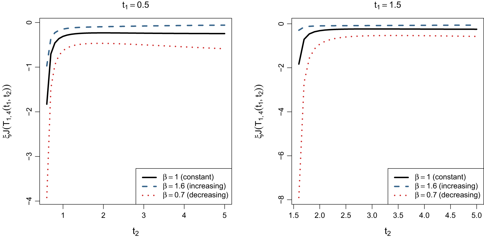


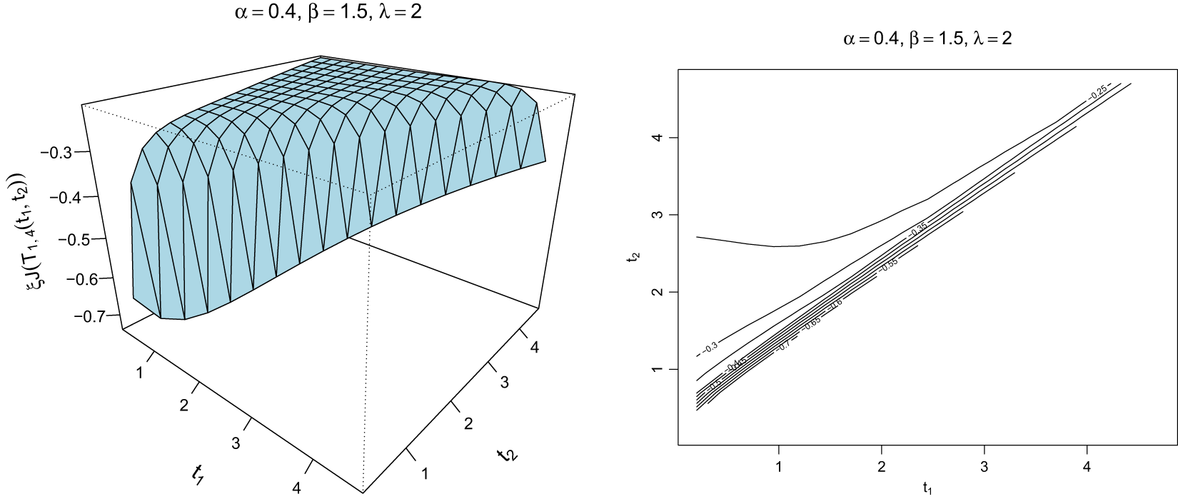


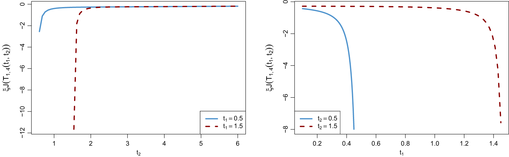


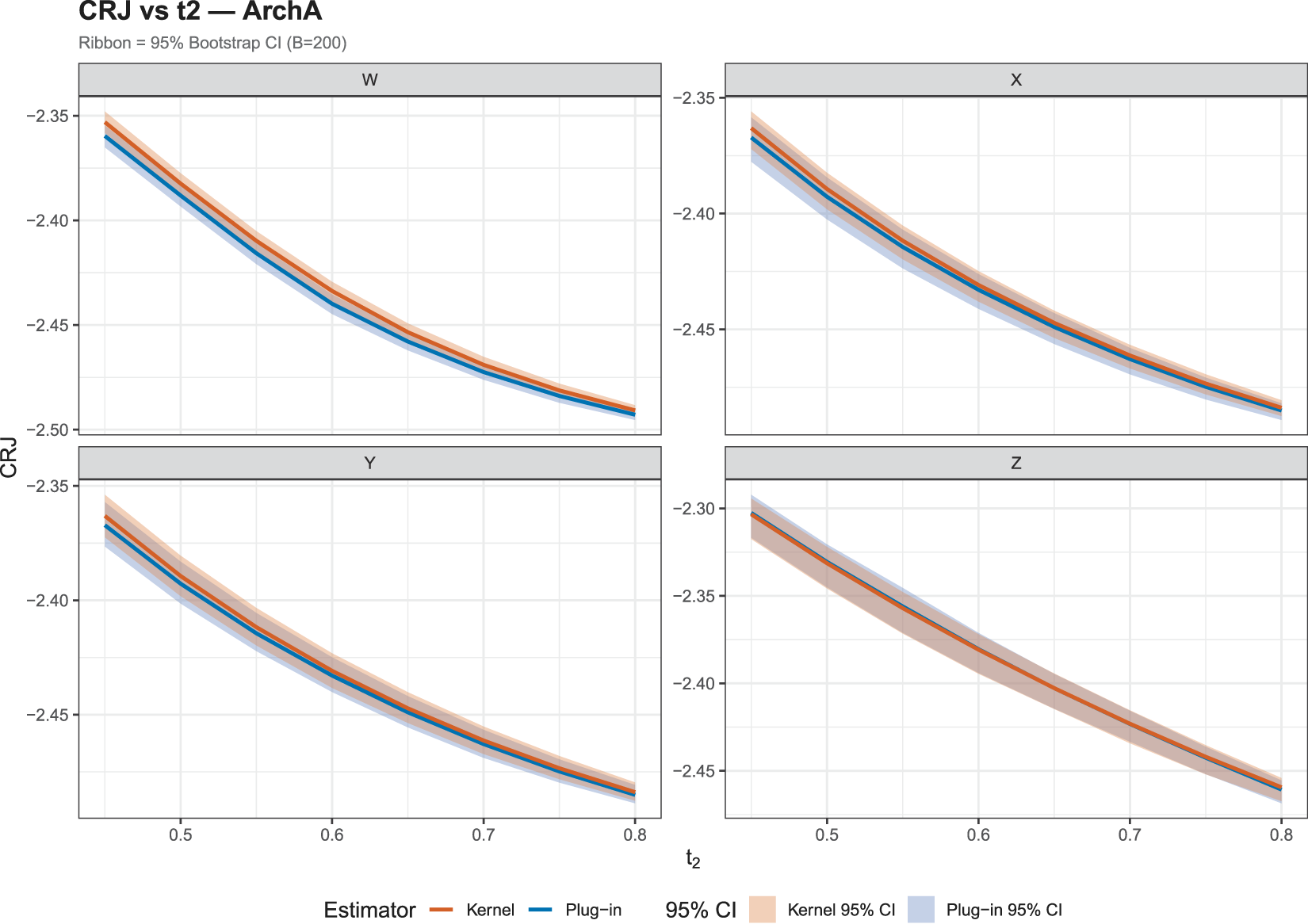


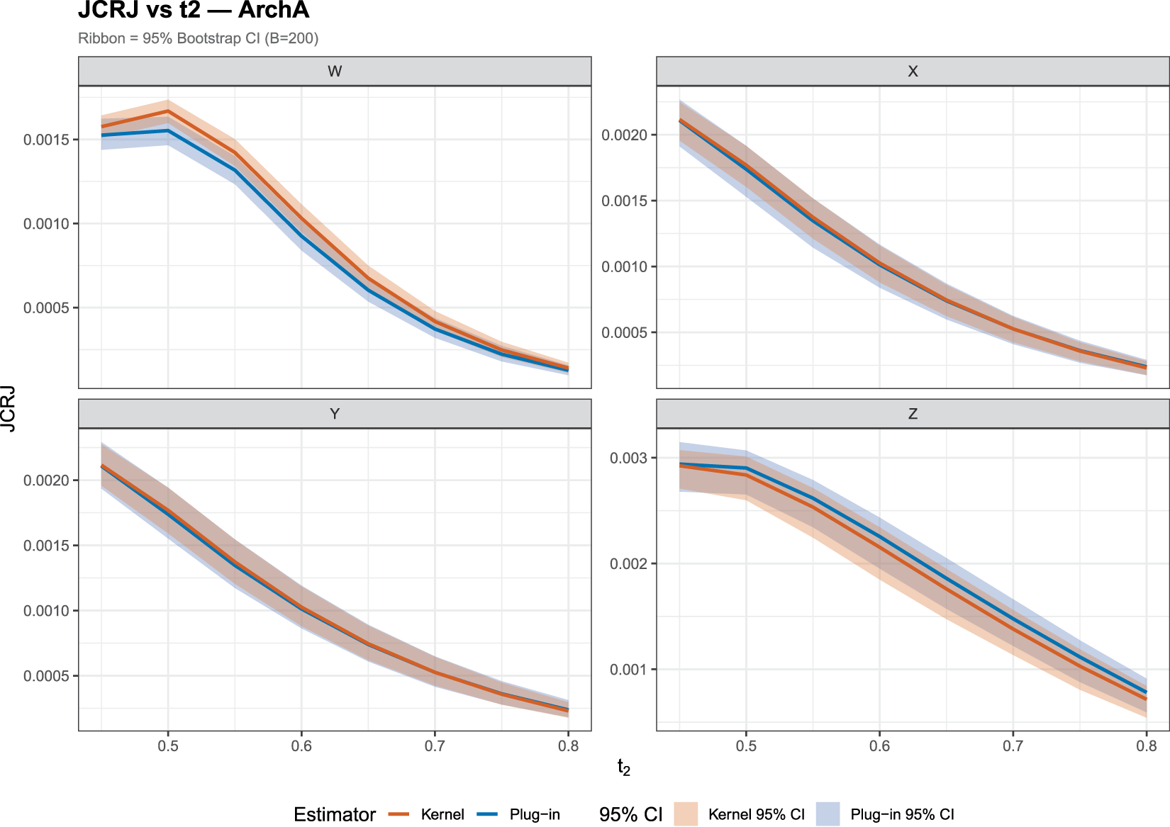


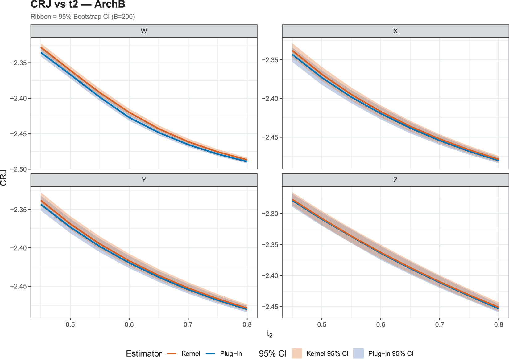


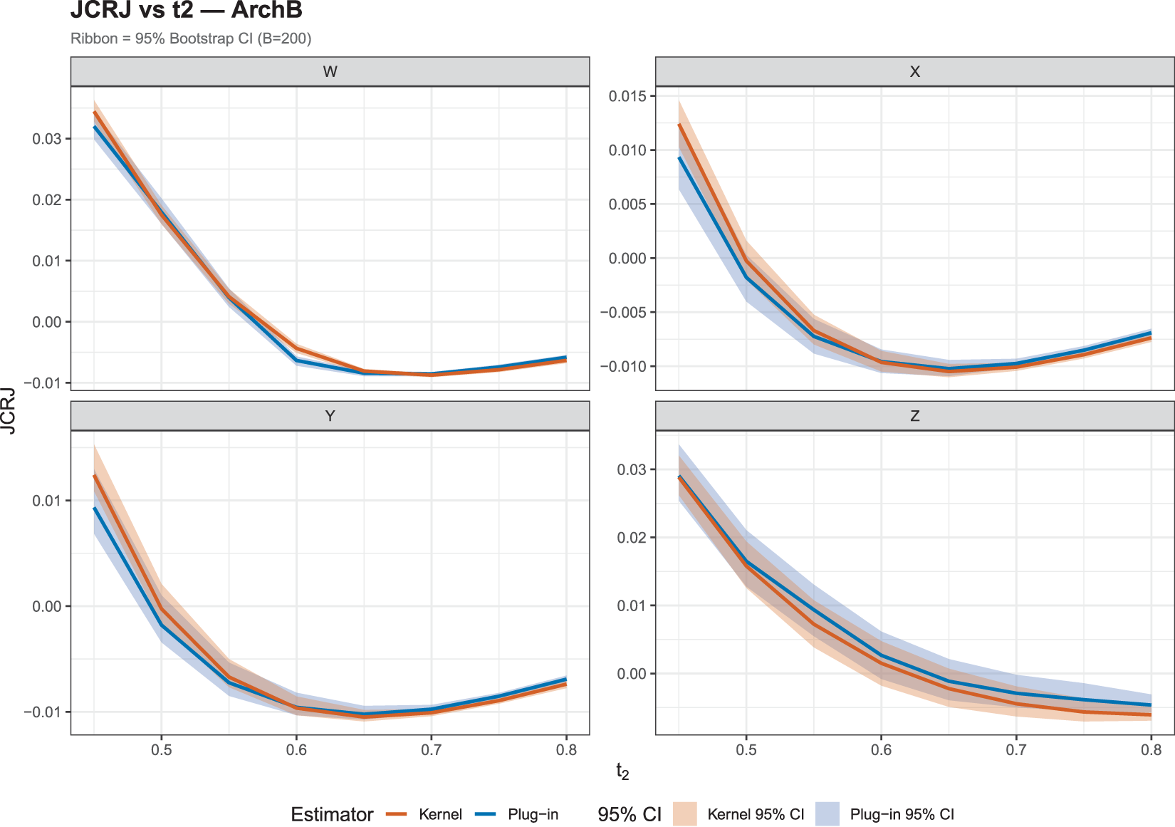


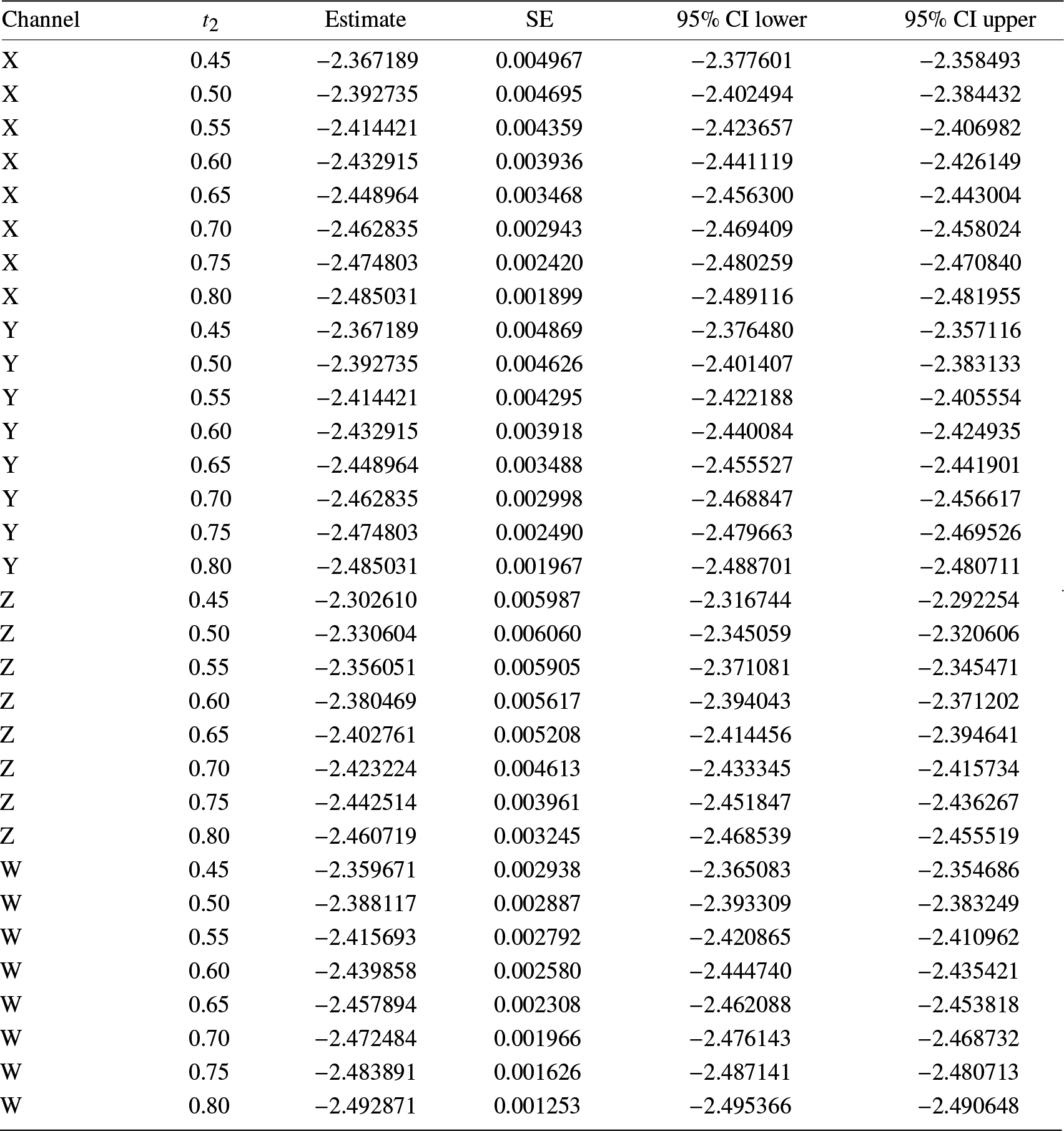

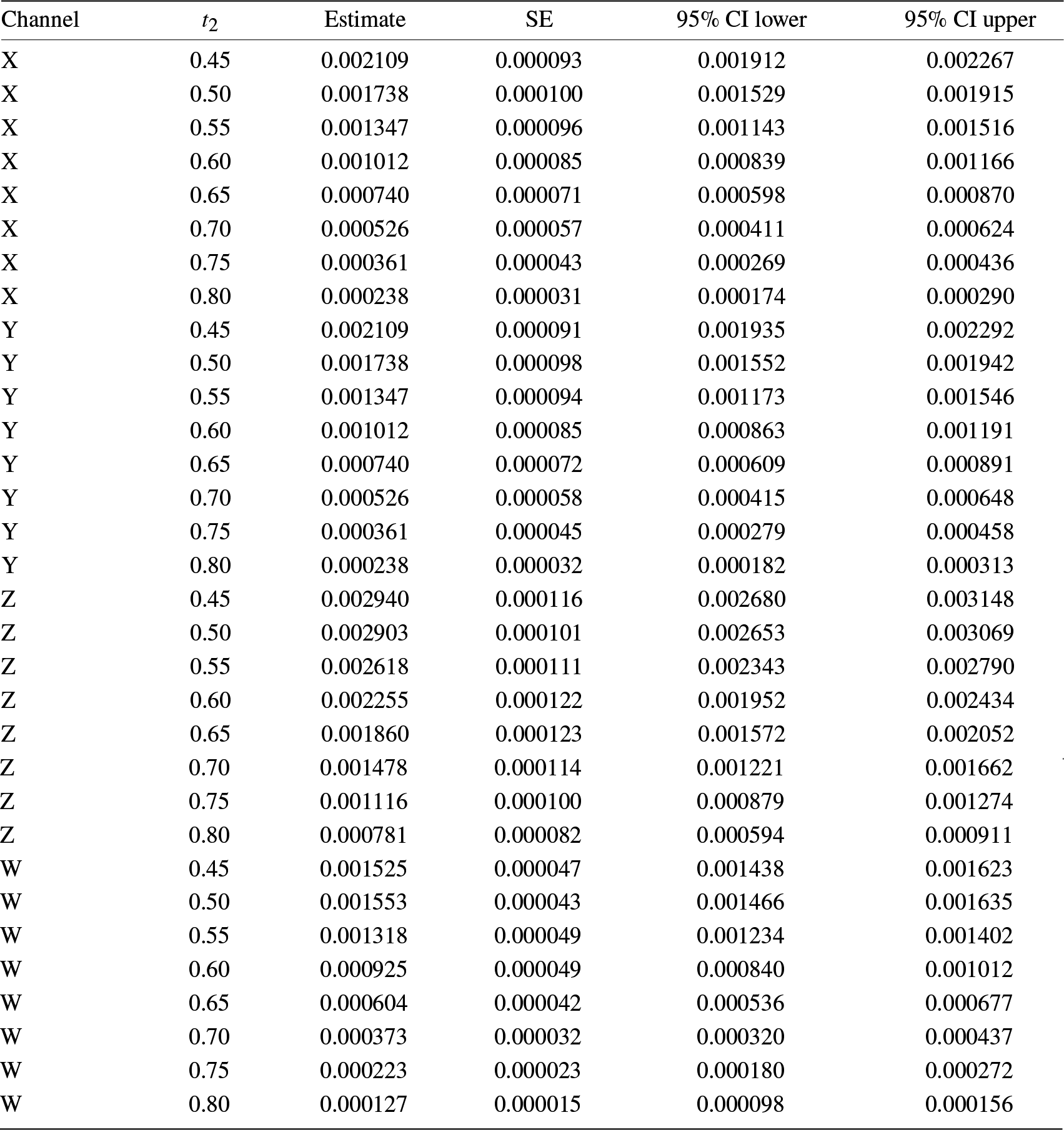

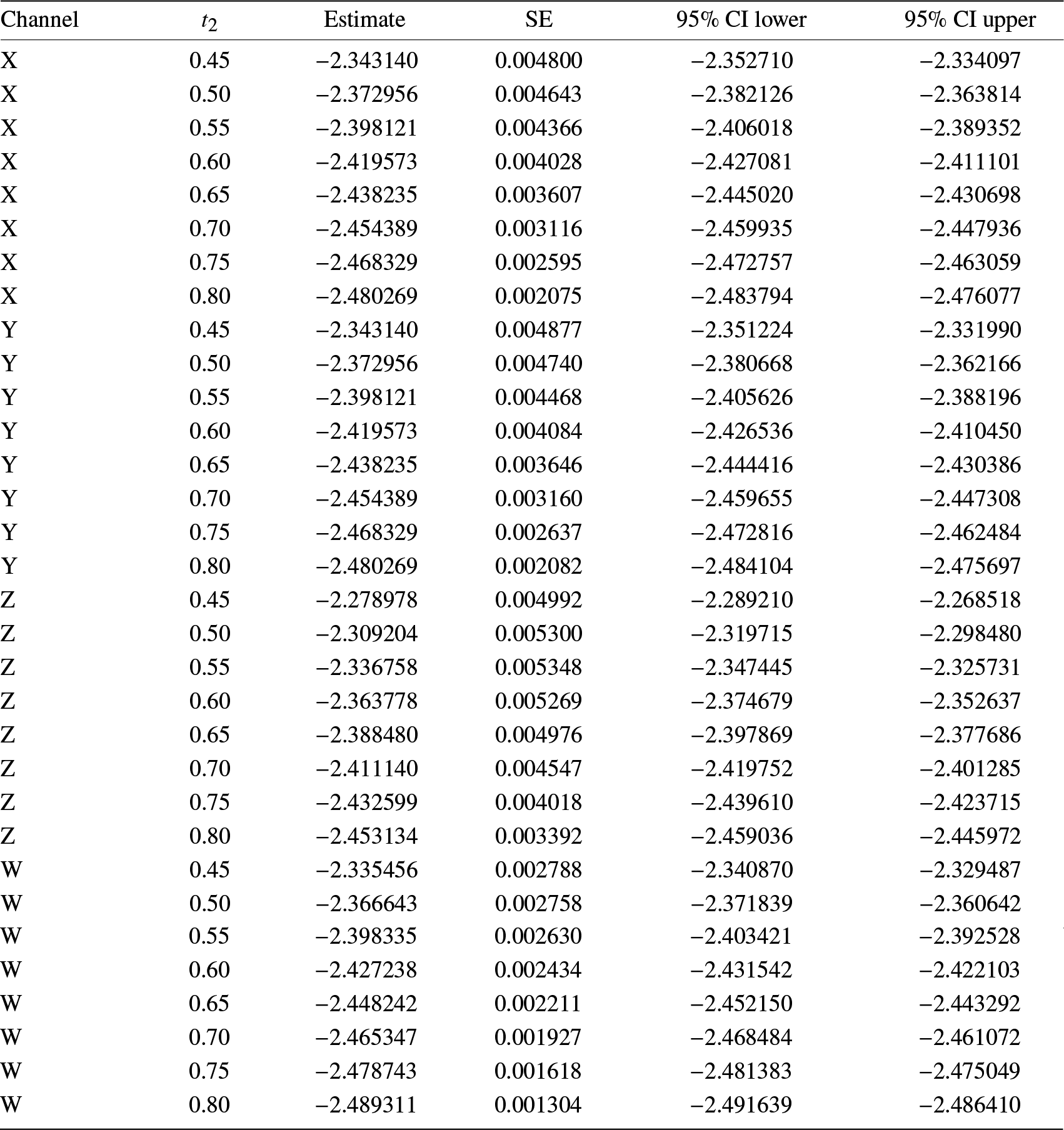


 Open access