Introduction

Recent glaciological and glacial-geological studies have shown that improved understanding of glacial systems requires better knowledge of how ice interacts with unconsolidated subglacial sediments. The current three-part series explores ice-sediment interactions in the absence of channelized surficial melt water reaching the bed and presents testable hypotheses about this situation; we do not consider the more difficult case of moulins supplying water to the bed.

In part I (Reference AlleyAlley, 1989), I hypothesized that in the absence of channelized melt-water supplies, if aquifers beneath a wet-based glacier on an unconsolidated bed were inefficient compared to the supply of basal melt water, then a distributed basal water system with low effective pressure would develop at the ice-sediment interface. In this paper I discuss how such a water system will affect partitioning of basal velocity between sliding, ploughing of clasts, and pervasive and discrete deformation of subglacial sediments. Then in part III (Reference Alley, Blankenship, Rooney and BentleyAlley and others, 1989) we use the known and inferred characteristics of Ice Stream B to make specific hypotheses about that ice stream.

Sliding

Most wet-based glaciers are restrained mainly by interaction with the roughness of their beds. An inefficient aquifer beneath a wet-based glacier will cause water to accumulate at the ice-bed interface until the accumulations become interconnected and allow drainage along that interface. Such an interconnected water system will have little effect on sliding velocity if it occupies only a small fraction, f, of the bed area and thus does not reduce the bed roughness significantly. Sliding resistance is a complicated function of size, shape, and arrangement of bed-roughness elements (Reference NyeNye, 1969; Reference WeertmanWeertman, 1969; Reference KambKamb, 1970; Reference FowlerFowler, 1987; Reference LliboutryLliboutry, 1987a,b; and earlier papers by most of these authors), but in general f must be large to allow fast sliding. For a given bed roughness, an increase in f requires an increase in water pressure so that water pressure exceeds ice normal stress over a larger fraction of the bed, as argued in part I.

The interconnected fractional area, f, must increase with the average water-film thickness, d, in a manner that depends on bed geometry. For a glacial till, a reasonable assumption is that the bed contains spherical clasts in different size classes, with all clasts in any class having the same size. The clasts with radii R_j occupy volume fraction of the till V_j for each of the j size classes, pores occupy volume fraction V_p, and

(1)

In an isotropic medium, areal fraction occupied on a section plane equals volume fraction for any size class (Reference UnderwoodUnderwood, 1970), and I will assume that this applies at the ice-till interface. I also will assume that each clast forms a hemispherical bump of radius R_j. With these assumptions, f the dependence of on d can be approximated for any specified grain-size distribution as

(2)

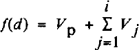
where i is chosen so that d #x2265; R_i the clast radius in the i th size class, but d ≤R_i+1 The base of the glacier is chosen as the base of the ice, so the porosity is assumed ice-free and the water system always occupies V_p.

It commonly is observed that tills contain a wide range of grain-sizes, from clay to boulders, and that the volume fractions are similar in size classes with logarithmically scaled radii (but often with bimodal peaks; Reference Sugden and JohnSugden and John, 1976, p. 228–31). One simple relation that meets these criteria is to divide clasts into seven size classes with radii R_j = 10⁻⁶, 10⁻⁵, … 10#x00B0; m, with one-tenth of the till volume in each of the seven size classes and with 30% of the volume in pores. This allows equation (2) to be approximated continuously as

(3)

where d is in meters. equation (2) does not allow for progressive submergence of individual clasts as d increases, whereas equation (3) is a crude attempt to do so. equation (3) is useful for calculating examples, and we will argue in part III that it is a reasonable assumption to use for Ice Stream B. Of course, the equivalent of equation (2) or (3) should be written as accurately as possible for any subglacial sediment under consideration.

Typical water-film thicknesses beneath a fast-moving glacier are likely to be 1–10 mm (e.g. Reference WeertmanWeertman, 1972; Reference Weertman and BirchfieldWeertman and Birchfield, 1982; part III), which from equation (3) gives f ≈; 0.7. From Weertman sliding theory (e.g. Reference WeertmanWeertman, 1964,1969), the sliding velocity u _s, under such conditions is approximately

(4)

where τ_b is the basal shear stress; the pre-factor can be evaluated from the bed roughness and depends on the controlling obstacle size, which typically is 1–10 mm (Reference WeertmanWeertman, 1964,1969). Using Weertman’s preferred constants, including an ice-hardness parameter of 0.17 bar⁻³ a⁻¹, and assuming that interference of stress fields around clasts reduces the effective bed roughness by a factor of 4 below that expected from the assumed roughness without interference (Reference Brown, Hallet and BoothBrown and others, 1987), the roughness assumed in equation (3) with a basal shear stress of tenths of a bar (10⁴-10⁵Pa) and with f = 0.7 (d = 1–10 mm), gives a sliding velocity of u_s = 0(1–10 m/a).

This calculated sliding velocity is low compared to similar calculations for typical bedrock beds considered by Weertman (e.g. Reference WeertmanWeertman, 1969) and other workers. The reason is that the spacing between obstacles of near the controlling size is small on a till bed as compared to a polished granite, for example.

Limited examples seem to support this contention that till beds cause glacier sliding to be slow. At Breidamerkurjökull, Reference Boulton and HindmarshBoulton and Hindmarsh (1987) showed that motion between markers in the base of the ice and the top of the underlying, deforming till accounts for only about 10% of the basal velocity of about ≤ 30 m/a; because of the finite size of the markers used, the sliding velocity is 4 3 m/a. Similarly, beneath Blue Glacier, Reference Engelhardt, Harrison and KambEngelhardt and others (1978) observed little or no slip between basal ice and the top of a “mobile sub-sole drift”, except during periods when the basal water was artificially overpressurized through drilling and the ice was floated off the bed. Notice, however, that natural water-layer thicknesses at the ice-bed interface were not measured at Breidamerkurjökull or at Blue Glacier.

It also is worth noting that clay-rich tills with few clasts ≥ 1 mm do occur naturally. If small clasts in such tills fail to aggregate into larger units, then and sliding velocities for such tills could be quite large. It is the common occurrence of clasts 0(1–10 mm) in radius that makes a till rough to ice.

Ploughing

In addition to sliding (see above) and pervasive bed deformation (see part I and below), a complete treatment of basal processes must consider the possiblity of ploughing. This is a transitional state between sliding and pervasive deformation in which individual clasts in contact with sliding ice are dragged through a till that is deforming locally but not pervasively. Ploughing was described by Reference Boulton, Dent and MorrisBoulton and others (1974), and was placed within a theoretical framework by Reference Brown, Hallet and BoothBrown and others (1987). In the discussion that follows, I briefly summarize the discussion of ploughing by Reference Brown, Hallet and BoothBrown and others (1987) and relate it to my treatment of sliding and bed deformation. I find that in most cases rapid ploughing is likely to lead directly to pervasive deformation so that ploughing need not be modeled separately; however, further data on till properties are needed to strengthen this conclusion.

First, I will simplify the ploughing model of Reference Brown, Hallet and BoothBrown and others (1987) and recast it in terms of the variables used in part I. Ploughing is initiated when the shear stress on a clast exceeds the local sediment strength on the yield surface for motion of that clast. As before, consider that the bed is composed of clasts in discrete size classes, with all clasts in a class having the same size. Let the average shear stress be τ_b, with clasts occupying fractional area s of the bed and water occupying fractional area f = 1 -s. In some arbitrary area A, clasts in the jth size class occupy area S _jA and support shear force τ_jA, so that the local shear stress on a clast in the v'th size class is τ_jA/(s_jA) = ^τ _j/S_j Also, let the local effective pressure on the failure surface for motion of a clast be N₁J and the local sediment strength be N_lJ/a₁ where a₁ is a geometric factor.

Reference Brown, Hallet and BoothBrown and others (1987) showed that ploughing occurs when the ploughing index , where

(5)

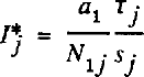
(Reference Brown, Hallet and BoothBrown and others (1987) called the ploughing index P* I use I* to avoid confusion here with pressure and stress terms P* Reference Brown, Hallet and BoothBrown and others (1987) also showed that

(6)

where ϕ is the angle of internal friction in degrees and cohesion has been assumed to be zero (Reference Brown, Hallet and BoothBrown and others, 1987).

The local effective stress can be approximated by N_1J = P_bj - P_w, where P_bj is the normal stress on the clast and P_w is the water pressure. Subtracting P_w from both sides of equation (A3) in part I and remembering that N = P_i - P_w yields

(7)

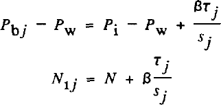
or substituting for ² from equation (22) in part I

(8)

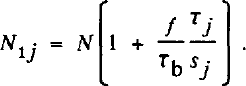
(Strictly, P_bj measures the vertical stress on a clast but N₁J measures the stress normal to the failure surface of a clast and adjacent materials. This could be corrected for by multiplying β by a numerical constant in equation (7). Reference Brown, Hallet and BoothBrown and others (1987, p. 8991) estimated K, the equivalent of β in equation (7), as between 0.1 and 0.44. For hydrostatically pressured water in subglacial sediments of Ice Stream B near the Upstream B camp, we estimate β ≈ 0.4 (part III). The extra constant in equation (7) thus should be near unity, and we omit it.)

It is convenient to define a new parameter, ζ_j as

(9)

It is the fraction of the average shear force (i.e. the force on a typical area A) that is supported by clasts in the jth size class.) Then combining Equations (5), (8), and (9) gives

(10)

The onset of ploughing occurs at I*_j=1, i.e. for

(11)

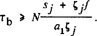
It is of interest to substitute typical numerical values into relationship (11). Reference WeertmanWeertman (1964) estimated that ζ_j= 1/3-1/2 for controlling obstacles, which will be the first to plough Reference Brown, Hallet and Booth(Brown and others, 1987). For the till bed introduced in equation (3), s_j = 0.1, and f = 0.3 for water occupying pore spaces only. Taking ζ_j = 1/2 and ϕ = 25° as typical for till Reference Brown, Hallet and Booth(Brown and others, 1987) yields a₁ = 2.7 and τ≥ 0.2N to allow ploughing.

An increase in shear stress above this minimum value will cause clasts of other sizes to plough and thus will increase the fraction of the bed ploughing. In the mathematical limit of the entire bed ploughing, the average behavior can be calculated by letting s_j = s and ζ_j = 1 in relationship (11), and remembering that s + f = 1. Then, from relationship (11), ζ_b > N/a₁ .

Ploughing of the entire bed is crudely equivalent to development of a continuous shear plane at the base of the ploughing clasts (but see below). It differs from pervasive deformation only in that continuous motion is restricted to the uppermost layer of clasts; deeper material disturbed by passage of large clasts returns to a static condition between disturbances. For ϕ = 25° and a₁ = 2.7 in a cohesionless till, the theory ofReference Brown, Hallet and Booth Brown and others (1987) predicts that ploughing of the entire bed would occur for ζ_b > 0.4N. In comparison, the criterion for pervasive deformation is

(12)

or for ϕ = 25°, ζ_b ≥ 0.5N.

Caution must be used in extending the ploughing theory of Reference Brown, Hallet and BoothBrown and others (1987) to high ploughing fraction. For example, the theory does not allow for overlap of failure surfaces of adjacent ploughing clasts, which would occur if most clasts were ploughing. Ignoring such complications, however, the calculations above suggest the not-so-startling result that a shear plane can be initiated in a till at a shear stress less than that required for pervasive deformation. Shear planes are observed in some tills (e.g. Reference MacClintock and DreimanisMacClintock and Dreimanis, 1964; Reference Boulton and HindmarshBoulton and Hindmarsh, 1987), lending credibility to this result. (It is unknown whether the processes of 100% ploughing causing a shallow shear plane in till actually occur.) However, this result suggests that there is a narrow range of basal shear stress (0.4 ≤ τ_b < 0.5N) in which ploughing of the entire bed can occur without pervasive deformation. This range is of similar width (0.1 to 0.2N) for tan ϕ = 0.2, and narrows to zero at tan ϕ = 0.75.

Another important complication must be introduced here. Laboratory experiments and field observations show that deformation of a till (or any granular material) causes it to dilate, and that a water-saturated till is weaker in its dilated state than in its collapsed, lodged state (Reference Boulton, Dent and MorrisBoulton and others, 1974; Reference Boulton and HindmarshBoulton and Hindmarsh, 1987). When deformation ceases, a dilated till tends to collapse back to its stronger, lodged state (Reference Boulton and DentBoulton and Dent, 1974). Reference Brown, Hallet and BoothBrown and others (1987) used ϕ = 25° as a typical value for till that is not actively deforming and suggested ϕ ≈ 11 (tan ϕ = 0.2) is a plausible minimum for till; Reference Alley, Blankenship, Bentley and RooneyAlley and others (1987a) suggested that ϕ ≈ 11° is the most likely value for the dilated, deforming till postulated beneath Ice Stream B. If tan ϕ ≈ 0.2 applies to a deforming till, then τ_b > 0.2N is sufficient to maintain deformation of an already deforming, non-cohesive till.

Reference Boulton, Dent and MorrisBoulton and others (1974) noted that a ploughing clast will dilate till locally by disturbing other clasts both adjacent and subjacent to it. If the time required for any locally dilated region to collapse back to its lodged state is long compared to the time until that region is disturbed by another ploughing clast, then that region will remain dilated and soft. The time between passages of ploughing clasts will decrease as the ploughing fraction increases with increasing shear stress. The possibility thus exists that ploughing will cause a transition to pervasive deformation at τ_b < 0.5N, the strength of lodged, undisturbed till. (It also is possible that ploughing will reduce the shear stress required to initiate further ploughing.)

I thus find that τ ≥C₁N will initiate ploughing, where C₁ ≈ 0.2, that an increased ploughing fraction requires C₁ > 0.2, but that pervasive till deformation will be sustained for C₁ ≈ 0.2. It is likely that C₁ passes through a maximum at some intermediate level of ploughing on the way to pervasive deformation, although any maximum must be less than or equal to 0.5, the value for pervasive deformation of a lodged till. To calculate the behavior between the onset of ploughing and pervasive deformation would require comparison of the disturbance rate from ploughing to the rate of collapse of dilated till following disturbance, but the collapse rate is unknown.

However, it is of some interest to calculate the disturbance rate. Consider the till bed introduced above, and suppose that ploughing is occurring only for clasts of radius 10 mm, which probably approximates the critical size on Ice Stream B. Such clasts occupy about 10% of the surface area of the ice-bed interface, and have a mean spacing in any direction (assuming isotropy) of about 120 mm (Reference UnderwoodUnderwood, 1970, p. 83). At a basal velocity of about 500 ma⁻¹ (typical of Ice Stream B), the average delay time between passage of clasts ploughing at a velocity close to the ice-stream velocity would be about 2 h at any spot. This delay time would be reduced slightly if I allowed for the increase in ploughing area caused by ploughing clasts pushing material ahead of them. Also, an increase in the fraction of the bed ploughing would reduce the delay, until there would be little delay if the entire bed were moving. Thus, if the time for a dilated till to collapse to a lodged state is long compared to 2 h for the ice velocity and till bed assumed here, ploughing would dilate the bed and lead to pervasive deformation with little or no increase in shear stress; however, if the collapse time is short compared to 2 h, the shear stress would need to increase substantially above the minimum for ploughing to mobilize a large fraction of the bed before pervasive deformation could begin. Unfortunately, I know of no available data to estimate the collapse time.

It is also of interest to ask under what conditions ploughing can lead to large basal velocities without pervasive deformation occurring. Reference Brown, Hallet and BoothBrown and others (1987) have presented indirect evidence for ploughing velocities of about 500ma⁻¹ without pervasive deformation beneath the former Vashon glacial lobe, whereas the direct evidence of Reference Boulton and HindmarshBoulton and Hindmarsh (1987) shows pervasive deformation without significant ploughing beneath Breidamerkurjökull.

As noted above, Reference Brown, Hallet and BoothBrown and others (1987) have proposed that ploughing clasts support a large fraction of the basal shear stress, occupy 0(10%) of the bed, and cover a size range centered on the controlling obstacle size (0(10⁻³–10⁻² m)). Reference Brown, Hallet and BoothBrown and others (1987) implicitly used a zero-viscosity (or a perfect-plasticity) model in which the ploughing velocity of a clast approaches the ice velocity if the shear stress on the clast equals the minimum value needed to cause motion. Real materials typically exhibit non-zero viscosity and finite exponent in power-law creep, such that strain-rate increases with stress; a Bingham model (velocity increasingly linearly with shear stress above the yield strength) or some other similar model is usually assumed (e.g. Reference Boulton and HindmarshBoulton and Hindmarsh, 1987). In either case, a large ploughing velocity without pervasive deformation would require a viscosity some orders of magnitude less than that measured at Breidamerkurjökull (Reference Boulton and HindmarshBoulton and Hindmarsh, 1987) or inferred for Ice Stream B (Reference Alley, Blankenship, Rooney and BentleyAlley and others, 1987b). To see this, consider the case of the UpB camp on Ice Stream B₁ where we have inferred that N ≈ 50 kPa, and tan ϕ ≈ 0.2 (Reference Alley, Blankenship, Rooney and BentleyAlley and others, 1987a; Reference Blankenship, Bentley, Rooney and AlleyBlankenship and others, 1987). The Bingham equation is

(13)

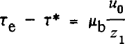
where τ_e is the effective shear stress causing deformation, τ* is the shear strength, u₀ is the velocity at the top of a deforming layer Z₁ thick, and u_b is the Bingham viscosity of the layer. For pervasive deformation

(14)

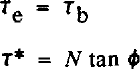
where cohesion again has been taken to be zero. For ploughing of the jth size class, from Equations (5)-(9)

(15)

At UpB, u_b ≈ 500 m a⁻¹, Z₁ ≈ 6m for pervasive deformation, and Z₁ ≈ 0.02 m for ploughing of controlling obstacles. The Bingham viscosity for pervasive deformation at UpB then is about 120 Pa a. Taking S_j0.1, f = 0.3, τ_j ϕ= 0.5 for ploughing of controlling obstacles only through a bed with water only in pore spaces then μ_b = 2.0 Pa a for ploughing through till with ϕ = 25° (lodged till) and μ_b = 3.2 Pa a for ϕ = 11° (dilated till); these values would be reduced to μ_b = 0.67 Pa a and μ_b = 2.9 Pa a if f = 0.7. Even letting N = 0, M_b = 4 Pa a is required to obtain u₀ = 500 m a⁻¹ by ploughing. If ploughing of controlling clasts is to yield a velocity similar to that inferred for pervasive deformation at UpB, then the till viscosity must be reduced by one to two orders of magnitude. (For comparison, typical Bingham viscosities for Breidamerkurjökull calculated from equation (13) and data from Boulton and Hindmarsh (1987) are around 3000 Pa a, or an order of magnitude higher than inferred at UpB, but Reference Fahnestock and HumphreyFahnestock and Humphrey (1988) reported a linear viscosity of about 30 Pa a beneath Columbia Glacier.) If more of the bed is allowed to plough, S_j will increase more rapidly than ζ_j on the ploughing fraction because the first size class to plough supports the largest fraction of the shear stress. This will decrease ( τ_ej- τ*_J) and thus require a lower Bingham viscosity to achieve the same ploughing velocity as calculated from equation (13).

This calculation places constraints on possible ploughing behavior, provided that ploughing obeys a Bingham-type deformation law. (Similar results to those above are also obtained using a linear-viscous model or the model preferred by Reference Boulton and HindmarshBoulton and Hindmarsh (1987).) For a given shear stress and water pressure at the ice-bed interface, the velocity from pervasive deformation of a till ≥0(1 m) thick is likely to be at least 1–2 orders of magnitude faster than that from ploughing through the same till. High ploughing velocities without pervasive deformation are likely only if the shear stress is less than the yield strength for pervasive deformation but the Bingham viscosity is at least J-2 orders of magnitude lower than that measured at Breidamerkurjökull or inferred at UpB.

The continuum treatment of granular materials used here introduces some ambiguity at large ploughing fractions. If clasts in many size classes are ploughing, the matrix through which they plough has a grain-size distribution and properties different from those of the bulk till. However, these differences are minimized when only one size class is ploughing. Note also that ploughing as modeled by Reference Brown, Hallet and BoothBrown and others (1987) occurs through till that is not deforming pervasively and thus is strong, but that I have used viscosities from soft, dilated, pervasively deforming till for comparison. Allowing for this difference would strengthen the conclusion reached above that high velocities through ploughing are unlikely.

To summarize, ploughing of clasts through lodged till will begin for τ i C₁N with C₁ ≈ 0.2, and all clasts in contact with the ice will plough for C₁ ≈ 0.4. Initiation of pervasive deformation of an undisturbed till requires C₁ ≈ 0.5, but pervasive deformation may be maintained for C₁ ≈ 0.2. An interesting, though unproven, hypothesis is that ploughing will dilate and soften till locally, allowing initiation of further ploughing and of pervasive deformation for values of C₁ somewhat smaller than specified here. High basal velocities through ploughing without pervasive deformation require lower Bingham viscosities in the ploughing layer than have been reported or estimated for modern tills. Based on these considerations, on our previous calculations that most velocity at the Upstream B camp in Ice Stream B arises from pervasive bed deformation (Reference Alley, Blankenship, Bentley and RooneyAlley and others, 1987a), and on the observations of basal motion dominated by pervasive deformation at Breidamerkurjökull (Reference Boulton and HindmarshBoulton and Hindmarsh, 1987), we will proceed in part III to model Ice Stream B assuming that ploughing does not contribute significantly to the basal ice velocity.

I do not have enough data to propose hypotheses for the differences between the inferred behavior of the Vashon glacier lobe (ploughing without pervasive deformation; Reference Brown, Hallet and BoothBrown and others, 1987) and of Ice Stream B (pervasive deformation; Reference Alley, Blankenship, Bentley and RooneyAlley and others, 1987a). Assuming that both inferences are correct, the difference might lie in till properties, the (lack of) availability of channelized, clean water from surface melt, or the (lack of) ice-marginal effects during glacier retreat. This is an area that clearly merits further study; the probability that abundant surficial melt water reached the bed of the Vashon glacier lobe at discrete points may provide a profitable starting place for such study.

Pervasive Deformation

General considerations

A sufficiently large basal shear stress will cause pervasive deformation in a subglacial sediment. Such deformation has been observed beneath Breidamerkurjökull (Reference Boulton and HindmarshBoulton and Hindmarsh, 1987) and Columbia Glacier (Reference MeierMeier, 1989), and inferred elsewhere. The velocity-tlepth profile and thickness of a pervasively deforming till layer are important in determining ice and till fluxes, and may be used in some cases to constrain the flow law for till; however, these topics have received little study to date.

Here I calculate velocity-depth profiles for the likely range of till properties and for both lithostatic and hydrostatic water-pressure gradients. The solutions obtained also apply if water-pressure gradients less than hydrostatic are specified; however, I do not consider the estimation of such gradients, which has been modeled by Reference Boulton and HindmarshBoulton and Hindmarsh (1987) and Reference ClarkeClarke (1987), among others. I exclude from consideration extrusion flow of till, which might occur if till viscosities were reduced to values typical of surficial debris flows by water pressures essentially equal to overburden pressures. Such flows could not be steady unless restricted to channels narrow compared to the ice thickness, owing to the mechanical instability of extrusion flow (Reference NyeNye, 1952). Extrusion flow has been modeled by Reference Mellors and WhillansMellors and Whillans (1986) and Mellors (unpublished), and its geomorphic implications have been discussed by Reference Boulton and HindmarshBoulton and Hindmarsh (1987). There is no direct evidence for the existence of such flow, however, and measured and inferred till viscosities at Breidamerkurjökull, Blue Glacier, UpB Reference Alley, Blankenship, Rooney and Bentley(Alley and others, 1987b), and Columbia Glacier (Reference Fahnestock and HumphreyFahnestock and Humphrey, 1988) are too high to allow significant extrusion flow (Reference Alley, Blankenship, Rooney and BentleyAlley and others, 1987b; Mellors, unpublished).

For this discussion, I adopt the coordinate axes shown in Figure 1, with the origin at the ice-till interface, z positive downward, and x positive in the direction of ice flow. The system is assumed to be two-dimensional: Reference BoultonBoulton (1979) discussed three-dimensional effects.

Fig. 1.

Coordinate axes for till-deformation calculations, with the origin at the ice-till inter face (or the top of the till if there is a significant water layer), z positive downward, and x positive in the direction of flow. The ice velocity is u_i, the sliding velocity is u_y the till velocity is u, the till velocity at z = 0 is u₀, and u_i = u_s + U₀ if there is no ice deformation. The pervasively deforming till thickness is Z₁.

If a fluid occupies communicating pore spaces in a material and is not flowing vertically, then the effective pressure is

(16)

where N₀ is the effective pressure at z = 0 and Δρ is the difference between the bulk density, ρ_b> and the pore-fluid density.

In a till that is not deforming, the pore-fluid density is the density of water, ρ_w, and the effective pressure assumes hydrostatic values given by

(17)

Effective pressure increases more rapidly with depth than this if downward porous flow occurs to a deeper, efficient aquifer.

Studies of debris flows suggest that, if the debris framework is deformed rapidly enough, water and fine clasts form an effective fluid in which larger clasts float (Reference Rodine and JohnsonRodine and Johnson, 1976;Reference Hampton Hampton, 1979). The fluid density then approaches the bulk density, and Δ ρ is reduced toward zero. In the limit of very fast deformation, Δ ρ = 0 and the fluid can be said to exhibit a lithostatic pressure gradient, giving

(18)

It is unknown whether equation (17), (18), or some intermediate case applies at the strain-rates that occur beneath glaciers lacking efficient deeper aquifers.

Deforming thickness

The thickness of a pervasively deforming layer can be limited by three factors: its yield strength, its strain-rate, or a change to a stronger material. The stronger material is the most obvious case; if a thin till directly overlies fresh granite, one would not expect the deforming layer to be thicker than the till.

Deformation of till causes it to dilate and soften (Reference Boulton, Dent and MorrisBoulton and others, 1974), but if the strain is not sufficiently rapid the dilated structure will collapse and the till will stiffen (Reference Boulton and DentBoulton and Dent, 1974). Alley and others (Reference Alley, Blankenship, Bentley and Rooney1986,1987a) proposed that this must place a limit on the possible deforming thickness; ice continuity limits potential ice velocity, and the minimum strain-rate for dilatancy then should limit the deforming thickness. This idea is speculative, but I will return to it below.

Yield-strength control is better established, and must figure in any full treatment of till properties. If effective pressure increases with depth, then yield strength also increases with depth, typically much more rapidly than does shear stress. If so, then the yield stress must increase above the shear stress at some depth in the till, stopping deformation.

The basal shear stress increases with depth in till according to

(19)

where α_i and _b are the down-stream slopes of the ice-air and ice-till interfaces, respectively, and ρ_j and h are the density and thickness of ice, respectively. For a horizontal bed (α_b = 0) and a surface slope α_i = 0.002, typical of Ice Stream B, T_b increases downward at about 20 Pa/m. By comparison, for hydrostatic water of density p_w = 1000 kg/m³ in till of bulk density ρ_b = 2000 kg/m³ and internal friction tan ϕ = 0.2, the yield strength increases downward at about 2000 Pa/m, or about two orders of magnitude faster. It is thus a good approximation to assume that T_b is constant in till; this can be called the thin-till approximation.

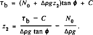
Making this approximation, then the basal shear stress equals the yield stress at depth z₂ given by

(20)

Velocity-depth profiles

Most proposed flow laws for shear deformation of water-saturated sediments have the form

(21)

where u is the velocity in the x direction, K_b is a constant (strictly speaking, K_b here is twice the value of K_b in equation (1), part I), and τ*, the yield strength, is given by

(22)

In the thin-till, lithostatic-water case where τ_b and N are independent of z, the velocity varies linearly with depth. If τ_b is constant but N varies with depth, equation (21) generates an interesting family of curves.

To investigate this family of curves further, it is convenient to make some definitions. Above, I defined z₂ as the depth at which the yield strength would equal the shear stress if the till were homogeneous and at least as thick as z_r Now I define Z₁ as the thickness of the deforming layer; that is,

(23)

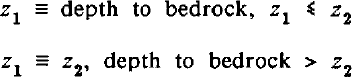
where “bedrock]” is any material under a till with a significantly higher yield strength. Combining Equations (20),(23) gives the general flow law for till as

(24)

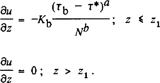
In addition, I define z₀ to be the depth at which the effective pressure is twice the value at the ice-till interface,

(25)

or an appropriate modification if downward water flow occurs. The variable z₀ measures how rapidly effective pressure increases with depth, Z₁ is the deforming thickness, and z₂ is the depth at which deformation would cease because of yield strength of the deforming layer.

Returning to equation (24) with z < Z₁, Equations (20) and (25) allow the deformation to be described by

(26)

which integrates to

(27)

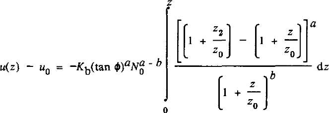
where u(0) = u ₀. At z = z₁, u drops to zero. Letting Z = Z_i in equation (27), solving for the constant terms and substituting back into equation (27) yields

(28)

A second integration gives the depth-averaged velocity, u , as

(29)

Equation (28) shows that the relative velocity u/u₀ occurs in a six-dimensional space defined by the powers a and b, and the depths z, z₀, Z₁, and z₂. I will restrict further attention to the case a = 1, appropriate to the Bingham and linear-viscous cases. Reference Boulton and HindmarshBoulton and Hindmarsh (1987) measured N, u₀, and z₁, and estimated τ_b for several sites beneath Breidamerkurjökull, and fitted the data using equation (24) with ∂u/∂z = u₀Z₁ and with τ* = 0 or τ* determined from their measurements. Their results were a = 1.33, b = 1.80 for τ* = 0, and a = 0.625, b = 1.25 for τ* > 0. They did not report errors on these determinations; based on my analysis of their data, I estimate standard errors of ±0.2–0.3 on a and b. If so, then a = 1 is consistent with their data. Also, a = 1 allows a good fit to the longitudinal profile of Ice Stream B (see part III). I wish to emphasize that I choose a = I as the mathematically simplest expression that is consistent with the available data, but I do not argue that a = 1 necessarily is exactly correct.

Taking a = 1, the integrations in Equations (28) and (29) then can be done for arbitrary values of the parameters b, z₀, Z₁, and z₂, and the variable z. Results are listed in Tables I and II in terms of dimensionless variables defined there. The general case is valid for b ≠ 1,2,3; logarithmic terms arise in b for b = 1,2 and in u for b = 1,2,3, as shown. In the limit of Z₁ = Z₂ (ω = 1), deformation occurs to bedrock. In the limit of z₂ → ∞ (ω →0), u and u are well behaved and give the behavior for a till with no yield strength.

Table I.

Equations for velocity-depth profiles in till with a = 1

Table 2.

Equations for average velocity in till with a = 1

The behavior for selected values of b and the dimensionless variables of Table I is plotted in Figures 2 and 3. Rapid velocity decrease with increasing depth near the top of the till is favored by large values of b and of χ = z ₀/z ₁ which lead to relatively low values of ö7 and thus of till flux. The variable ω = Z₁/z₂ determines how rapidly the velocity decreases to zero near the base of the deforming layer; large ω requires that the deeper velocities be almost asymptotic to zero, requiring rapid velocity decrease with depth near the top of the deforming layer and thus small u However, the velocity-depth profile is less sensitive to ω than to b or x.

Fig. 3.

Depth-averaged velocity of pervasive deformation, u , normalized by u₀, plotted against x (= chi), for different values of x (ω= omega); all variables are defined in the caption to Figure 2. Each plot contains curves for b = 0, 1, 2, 3, and 5 (indicated to the lower right of the appropriate curve) assuming a = 1. The average velocity (and thus till flux) decreases with increasing b and ω and with decreasing x. The likely values of x, b, and ω discussed in this paper and in part III give u /u ≈ 0.1–0.5.

Fig. 2.

Velocity-depth plots. Plots of u/u₀ (horizontal till velocity normalized by velocity at top of till) are shown against relative depth, ψ (= psi = z/z₁ where Z₁ is the base of pervasive deformation and z is the depth). The exponent a = 1 in equation (24), and each column of plots is headed by the value of the exponent b used in that column; each row uses the value of ω shown at the left (ω = omega = Z₁Zz_v where z₂ is the depth at which the shear stress would equal the strength of the pervasively deforming till). Each plot contains curves for x = 0.01, I, 10, 100, where x = Z₀/z₁ and z₀ is the depth at which the effective pressure, N, in the till is twice the value at the ice-till interface, N₀. Curves for b = 0 are independent of x as shown. For b ≥ 1, curves are identified by x values placed to their lower right, unless otherwise indicated. The limiting case of x = 0, b > 0 gives a curve plotting on the top and left coordinate axes (as does b →∞); the x = 0.01 curves for b = 5 are close to this behavior. In the limit of x → ∞, curves with b ≠ O become identical to the b = 0 curves; the x = 10 and x = 100 curves for small b are essentially at this limit and plot quite close together. All curves are monotonie and smooth; slight irregularities in the figure arise from the computerized plotting package used.

In principle, if till deformation obeys equation (24) with a = 1, then one can measure z₀, z₁ Z₂ (possibly), and u(z), and determine b and Z₂ (if necessary) from comparison between the data and Figure 2. Although no-one has measured all of the necessary parameters in a deforming till and the applicability of equation (24) is open to question, analysis of the seminal data set of G.S. Boulton and co-workers from Breidamerkurjökull (e.g. Reference Boulton, Dent and MorrisBoulton and others, 1974; Reference BoultonBoulton, 1979;Reference Boulton and Hindmarsh Boulton and Hindmarsh, 1987) suggests that this method is workable but difficult.

In Figure 4, I show the velocity-depth data of Reference Boulton and HindmarshBoulton and Hindmarsh (1987, fig. 2) re-plotted according to the variables used here. In each case, I have estimated the velocity at the top of the till, u₀, by interpolating linearly between the velocities of the lowermost marker in the ice and the uppermost marker in the till in Reference Boulton and HindmarshBoulton and Hindmarsh (1987, fig. 2). I have also assumed that the thickness of the deforming layer (z₁ = z₂) is the till thickness above the lowermost marker placed by Reference Boulton and HindmarshBoulton and Hindmarsh (1987), although slow motion across discrete shear planes is reported to occur below the lowermost markers.

Fig. 4.

Measured velocity-depth profiles of till beneath Breidamerkurjökull (Reference Boulton and HindmarshBoulton and Hindmarsh, 1987, fig. 2) plotted on the scale defined in the caption to Figure 2, Numbers 1–4 refer to the arrays 1–4 shown in Figure 2 of Reference Boulton and HindmarshBoulton and Hindmarsh (1987). The inflection points that I identify with the base of pervasive deformation are indicated by arrows.

Comparison of Figures 2 and 4 shows immediately that the real world is more complicated than assumed in equation (24). Some of the “wiggles” in the velocity-depth profiles in Figure 4 are caused by proximity to large rigid clasts (e.g. arrays 3 and 4 near Z/Z₁ = 0.6, where the shear strain-rate decreases almost to zero; Reference Boulton and HindmarshBoulton and Hindmarsh, 1987). Also, transverse flow may have minor effects on velocity-depth profiles (Reference BoultonBoulton, 1979). However, the rapid downward decrease in velocity (large shear strain-rate) near the base of each curve requires a different explanation.

The inflection points (that is, the points where the shear strain-rates pass through minima, which I term inflection points for convenience (Fig. 4)) in the velocity-depth profiles occur at (array 4) or just above (arrays 1, 2, 3) the depths where Reference Boulton and HindmarshBoulton and Hindmarsh (1987) observed a downward change in mode of deformation from pervasive creep to shear on discrete planes. The till porosity is relatively high and decreases slowly with increasing depth above the inflection point, but decreases rapidly with depth from near the inflection point to the bottom of the profile (Reference Boulton and HindmarshBoulton and Hindmarsh, 1987, fig. 4a).

I suggest that these observations demonstrate the existence of a minimum strain-rate required to maintain dilation (Alley and others, Reference Alley, Blankenship, Bentley and Rooney1986,1987a). Remember that till can be transformed from a compact, strong state to a dilated, weak state by strain in the presence of excess water (so that the material remains saturated) and this is reversible if the pore water can escape during compaction (Reference Boulton and DentBoulton and Dent, 1974). It is reasonable to expect that if the strain-rate in a dilated material becomes too low, then the collapse process will be dominant over dilation, causing the till to lose porosity and gain strength. The feed-back related to this (slow strain → collapse → stronger till → slower strain) should cause the transition zone between soft, dilated, pervasively deforming till and strong, collapsed till without pervasive deformation to be relatively thin. However, discrete shearing is possible under conditions that suppress pervasive deformation (see discussion on ploughing, above), and thus might occur in and just below this transition zone. Calculations by J.S. Walder (personal communication, 1988) suggest that such slow shearing at the base of a pervasively deforming till is possible over consolidated rock as well.

The minimum strain-rate hypothesis then predicts that pervasive deformation will cease when the strain-rate falls to some critical value (or the effective pressure and shear strength rise to some critical value compared to the shear stress), that the strain-rate just above this depth will exceed the expected strain-rate just above the depth where τ = τ* (z = z₂) in equation (24), that the porosity will decrease rapidly near this depth, and that discrete shearing may occur near and below this depth. The agreement between hypotheses and observations suggests strongly that a minimum strain-rate for dilation does exist and is reached near the inflection points shown in Figure 4.

This discussion suggests that tan ϕ (and possibly C and N) are inverse functions of du/dz, and that the true flow law is likely to be a very complicated entity, as discussed by Reference ClarkeClarke (1987). It remains possible, however, that equation (24) (and its solutions in Table I) can be modified to provide a reasonable approximation of the actual behavior. Reference Boulton and HindmarshBoulton and Hindmarsh (1987) showed that the porosity decreases downward only slowly in the upper *70% of the deforming layer before dropping rapidly into the zone of discrete shearing, and porosity should be a good proxy for till strength for a given till. Suppose we let z ≡ Z₃, be the depth to the bottom of the relatively homogeneous upper part of the layer, so that the strain-rate falls to the minimum value to maintain dilation ( ) at z = z₃. Assume further that tan ϕ, C, and z₀ are independent of Z in this upper, pervasively deforming region. Then equation (23) can be rewritten as

(30)

and equation (24) still describes pervasive deformation.

Here Z₁ is the thickness of the pervasively deforming layer, Z₂ is the depth at which the yield strength of this pervasively deforming layer would equal the basal shear stress, and z₃ is the depth at which the pervasive deformation ceases (or would cease) because of strain-rate control. This means that Z₁ ≤ Z₃ ≤ Z₂.

With these assumptions, Figure 2 and Table I still describe the deformation, but the variable ω = Z₁/z₂ cannot be larger than Z_b/z₂ and thus is less than 1. Also, the velocity u must be understood as arising from pervasive deformation; discrete shear at the base of the pervasively deforming layer provides an additional velocity just as discrete shear at the top of the layer provides the additional sliding velocity.

The data of Reference Boulton and HindmarshBoulton and Hindmarsh (1987) show that the sediment porosity (and by inference, the softness of the sediment) does decrease slowly downward in the pervasively deforming layer. Thus, calculations following equation (24) and using the appropriate values of constants will underestimate the curvature of measured velocitydepth profiles. Stated differently, if z₀, z₁ z₂, and z₃ are known and b is chosen to provide the best match between calculated and observed velocity-depth profiles, then this value of b will place an upper limit on the true value.

Bearing this in mind, we now can attempt to fit the velocityiepth profiles for the pervasively deforming layer at Breidamerkurjökull, and thus to constrain the flow law for till. The inflection points in Figure 4, which I argue are good approximations of z₃, occur at ψ = z/z₁ ≈ 0.8 (array 1), 0.6 (array 2), 0.75 (array 3), and 0.7 (array 4). Defining these points to be z_s and the deformational velocity, u, at these points to be zero yields the curves shown in Figure 5. From the data and calculations of Reference Boulton and HindmarshBoulton and Hindmarsh (1987), the effective pressure at the ice-till interface is N ≈ 40 kPa, and the effective pressure would double at z₀ ≈ 3 m. The pervasively deforming layer is Z₁ ≈ 0.4 m thick, so x = Z₀/z_l ≈ 7.

Fig. 5.

Curves from Figure 4 above the inflection points, recalculated so that u = 0, ψ = 1 at the inflection points. The curve labeled “model” is calculated from equation (28) with a = 1, b = 2, x=7, and ω = 0.9.

The reader can compare Figures 2 and 5 to estimate which values of ω and b in Figure 2 predict curves similar to those in Figure 5. I do not try a detailed, statistical curve-fitting exercise because of the large variability in the observed profiles and the uncertainties introduced by depth variation of till properties, the presence of large, rigid clasts, and the likely occurrence of transverse flow. However, by inspection, I find that b ≈ 2–3, ω ≈ 0.9 provides a good fit. Reducing ω requires an increase in b to maintain reasonable agreement between model and observed curves, but the quality of the fit deterioriates slowly from (ω, b = (0.9, 2) to (0.5, 5), and becomes very bad for smaller ω. It is notable that the values I find that give a good fit (0.9, 2–3) give b close to what we would expect based on the between-site fit of Reference Boulton and HindmarshBoulton and Hindmarsh (1987), especially if we reduce b slightly from 2–3 to allow for the effect of slow variation of till properties with depth in the pervasively deforming layer. I therefore suggest that a curve-fitting exercise such as this is not a sensitive test for flow-law constants, but does aid in constraining these constants.

If we accept (ω, b) = (0.9, 2) as a working hypothesis, two further calculations suggest themselves. First, at z = Z₁, the slope of the model curve gives as an estimate for , the minimum strain-rate required to maintain pervasive till dilation and deformation.

Secondly, the estimate ω ≈ 0.9 can be used to constrain the yield strength of the dilated till. Because ω = Z₁Zz_i and Z₁ ≈ 0.4 m, Z₂ ≈ 0.45 m. At this point, T_b = N tan ϕ+ C for the dilated till. Reference Boulton and HindmarshBoulton and Hindmarsh (1987) (also see Reference Boulton and DentBoulton and Dent, 1974; Reference Boulton, Dent and MorrisBoulton and others, 1974; Reference BoultonBoulton, 1979) measured C ≈ 4 kPa, tanϕ≈ 0.625, and presented data that allow us to estimate N(0.45 m) ≈ 46 kPa; however, the method used to measure tan ϕ probably over-estimates that number (Reference Alley, Blankenship, Bentley and RooneyAlley and others, 1987a). If T_b were known accurately, then we could use N(Z₂), C, and T_b to estimate tan ϕ. Unfortunately, the measurements of Reference BoultonBoulton and Hindmarsh (1987) were made within a few ice thicknesses of the glacier terminus, where effects of longitudinal deviatoric stresses (Reference NyeNye, 1967) or back-pressure from small push moraines can cause the basal shear stress to deviate significantly from the usual assumption τ_b = p₁gha, where ρ_i, h, and ρ are the ice density, thickness, and surface slope, respectively. (Reference Boulton and HindmarshBoulton and Hindmarsh (1987) did not report the method they used to estimate τ_b; possible uncertainties from near-terminus effects probably broaden the likely errors in their determination of flow-law exponents beyond the limits I cited above.) Nevertheless, if we assume as an exercise that the usual basal shear-stress formula applies, then T_b ≈ 30 kPa and tan ϕ = 0.56. A similar calculation with ω = 0.5, z₂ = 0.8 would give tan ϕ = 0.51. These calculations certainly involve large errors, but in principle calculations such as these can be used to constrain till strength better.

Hypotheses

My discussion of velocity-depth profiles in deforming tills has covered a number of aspects. More than anything else, I believe it demonstrates the need for well-designed, direct studies of subglacial deformation. The studies of Boulton and co-workers (e.g. Reference Boulton and DentBoulton and Dent, 1974; Reference Boulton, Dent and MorrisBoulton and others, 1974; Reference BoultonBoulton, 1979; Reference Boulton and HindmarshBoulton and Hindmarsh, 1987) clearly are the standard against which all other efforts will be judged, but it is equally clear that this single project does not constrain the full range of possible behaviors.

Despite our large uncertainties regarding till properties, the discussion above does provide some information on till deformation. It also allows me to propose the following hypotheses, most of which should be testable in future field programs:

Acknowledgements

I thank CR. Bentley, D.D. Blankenship, T.J. Hughes, and S.T. Rooney for helpful comments on the manuscript, and I am indebted to J.S. Walder for numerous suggestions and criticisms, not all of which are answered satisfactorily here. I thank A.N. Mares for manuscript preparation, and C.R. Alley for computerized figure drafting. This work was supported by the U.S. National Science Foundation under grant DPP87–16016. This is contribution number 498 of the Geophysical and Polar Research Center, University of Wisconsin-Madison.