1. Introduction
The study of Bernoulli percolation on
 $\mathbb{Z}^d$
is more than 60 years old and the existence of a non-trivial phase transition for
 $d\geq 2$
is well established for the model and several of its variants, but the exact value of the critical parameter
 $p_\mathrm{c}$
is seldom known. A celebrated result of Kesten [Reference Kesten11] proved that the critical probability in Bernoulli bond percolation on
 $\mathbb{Z}^2$
is
 $\frac12$
. Besides that, the exact critical probability was established only for some planar lattices where symmetry and duality properties are well explored. On the other hand, for dimensions
 $d\geq 3$
, there is not much hope of finding exact values for the critical probability. Several non-rigorous estimates, either via Monte Carlo methods (see the very efficient algorithm in [Reference Newman and Ziff14]) or statistical estimates based on a comparison with dependent percolation (see [Reference Bollobás and Riordan2, Section 6.2] for an overview) are present in the literature, but rigorous bounds are rare (see, in different contexts, [Reference Campanino and Russo3, Reference Liggett12, Reference Wierman15, Reference Wierman and Parviainen17]). In this paper, we focus on finding rigorous upper bounds for site and bond Bernoulli percolation on
 $\mathbb{Z}^d$
for every
 $d\geq 3$
, in both the oriented and non-oriented cases. Although those bounds are still far from the values obtained from Monte Carlo simulations, we believe that most of them are the best rigorous upper bounds in the literature.
The primary tools we use are dynamical couplings between the models we seek to understand and models where bounds or precise values for the critical probabilities are known. Such couplings are now a classic tool in percolation theory, but its extensive use to establish upper bounds on critical parameters for all dimensions, we believe, is new. In [Reference Chayes and Schonmann4], the authors establish inequalities between the critical thresholds of site and bond non-oriented percolation through the use of differential inequalities.
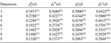
The remainder of the text is organized as follows: In Section 2 we precisely define the models; state the main results; and, in Subsection 2.3, we give a numerical table with upper bounds for the critical probabilities in homogeneous Bernoulli percolation models for dimensions up to
 $d=9$
. In Section 3 we establish some dynamical couplings and in Section 4 we prove the theorems.
2. The models and main results
For
 $d \geq 1$
, the underlying graph for all the models will be the d-dimensional hypercubic lattice in which the set of vertices is
 $\mathbb{Z}^d$
and the set of edges is the set of non-ordered pairs
 $E(\mathbb{Z}^d) \,:\!=\, \{ \langle v, u \rangle \colon v, u \in \mathbb{Z}^d \text{ and } |v-u| =1\}$
. We abuse notation and denote this graph simply by
 $\mathbb{Z}^d$
. Throughout the text, for each
 $x \in \mathbb{R}$
we will denote by
 $\lfloor x \rfloor$
the largest integer smaller than or equal to x.
This section is divided into two subsections. The first is devoted to bond percolation models, while the second is devoted to site percolation models.
Before we proceed with formal definitions of the models, we introduce some notation that will be useful.
Definition 1. Given two real numbers
 $a \in (0,1)$
and
 $b > 1$
, we denote by
 $\mathrm{Sol}(a,b)$
the unique solution of
 $x = a[x + (1-x)^b]$
in the interval (0,1).
Observe that for every x in the interval (0,1), the right-hand side of the equation is smaller than a, therefore
 $\mathrm{Sol}(a,b) < a$
. Writing
 $f(x) = x - a[x + (1-x)^b]$
, we have
 $f(0) = -a < 0$
and
 $f(1) = 1 - a > 0$
. Moreover, observe that
 $f'(x) = (1 - a) + ab(1-x)^{b-1} > 0$
for every
 $x \in (0,1)$
, which guarantees the uniqueness of
 $\mathrm{Sol}(a,b)$
.
2.1. Bond percolation
Given
 $p \in [0,1]$
, consider a family of independent random variables
 $\{X_e\}_{e \in E(\mathbb{Z}^d)}$
where, for each
 $e \in E(\mathbb{Z}^d)$
,
 $X_e$
has Ber(p) distribution. Let
 $\mu_e$
be the law of
 $X_e$
, and let
 $\mathbb{P}_{p} \,:\!=\, \prod_{e \in E(\mathbb{Z}^d)} \mu_e$
be the resulting product measure. We declare an edge e to be open if
 $X_e=1$
and closed otherwise.
We first consider the non-oriented case and denote by
 $\{x \leftrightarrow y\}$
the event where
 $x, y \in \mathbb{Z}^d$
are connected by an open path, i.e. there exist
 $x_0, \dots, x_n$
such that
 $x_0 = x$
,
 $x_n =y$
, and each
 $\langle x_{j-1}, x_j \rangle$
belongs to
 $E(\mathbb{Z}^d)$
and is open for
 $j=1, \dots, n$
. Let
 $\mathcal{C}^\mathrm{b}_0 \,:\!=\, \{x \in \mathbb{Z}^d\colon 0 \leftrightarrow x\}$
be the open cluster of the origin, and
 $|\mathcal{C}^\mathrm{b}_0|$
its size.
We define the percolation probability by
 $\theta^\mathrm{b}_d(p) \,:\!=\, \mathbb{P}_p(|\mathcal{C}^\mathrm{b}_0|= \infty)$
. The critical point for the non-oriented bond Bernoulli percolation model will be denoted by
 \begin{equation*} p_\mathrm{c}^\mathrm{b}(d)=\sup\big\{p \geq 0 \colon \theta^\mathrm{b}_d(p)=0\big\}.\end{equation*}
We now consider the oriented case. Let
 $\{e_1, \dots, e_d\}$
be the set of positive unit vectors of
 $\mathbb{Z}^d$
. We denote by
 $\{x \rightarrow y\}$
the event where
 $x, y \in \mathbb{Z}^d$
are connected by an oriented open path, i.e. there exist
 $x_0, \dots, x_n$
such that
 $x_0 = x$
,
 $x_n =y$
, and, for each
 $j=1, \dots, n$
, we have
 $x_j - x_{j-1} \in \{e_1, \dots, e_d\}$
and
 $\langle x_{j-1}, x_j\rangle$
is open. Let
 $\vec{\mathcal{C}}^\mathrm{b}_0 \,:\!=\, \{ x \in \mathbb{Z}^d \colon 0 \rightarrow x\}$
be the oriented open cluster of the origin, and
 $|\vec{\mathcal{C}}^\mathrm{b}_0|$
its size.
Analogously, we define
 $\vec{\theta}^{\mathrm{b}}_d(p) \,:\!=\, \mathbb{P}_p(|\vec{\mathcal{C}}^\mathrm{b}_0|= \infty)$
to be the corresponding oriented percolation probability, and we denote the critical point for the oriented bond Bernoulli percolation model by
 \begin{align*}\vec{p}_\mathrm{c}^{\mathrm{b}}(d)=\sup\{p \geq 0 \colon \vec{\theta}^{\mathrm{b}}_d(p)=0\}.\end{align*}
For the non-oriented bond percolation model, our result is the following.
Theorem 1. Consider non-oriented bond Bernoulli percolation and let
 $p^{\ast}(d)$
be the unique solution in
 $(0,1)$
of
 \begin{equation} \prod_{i=0}^2\big(1-(1-p)^{\lfloor({d+i})/{3}\rfloor}\big) = 2-\sum_{i=0}^2(1-p)^{\lfloor({d+i})/{3}\rfloor}. \end{equation}
Then, for every
 $d\geq 3$
, we have
 $p_\mathrm{c}^\mathrm{b}(d) \leq p^{\ast}(d)$
.
To state our result for oriented bond percolation model, we recall Definition 1.
Theorem 2. Consider oriented bond Bernoulli percolation on
 $\mathbb{Z}^d$
. The following three statements hold:
-
(i) If d is even, then
 $\vec{p}^\mathrm{b}_\mathrm{c}(d) \leq 1-\big(\frac13\big)^{2/d}$
.
-
(ii) For
$d \geq 4$
,
\begin{align*} \vec{p}^\mathrm{b}_\mathrm{c}(d) \leq \frac{1}{d}+\frac{C_d}{d^2}, \qquad \text{where} \quad C_d=1+\frac{8}{d}+\frac{d^{5/2}}{(\sqrt{2\pi})^{d-1}}\left[\frac{d-1}{d-3}\right]{\mathrm{e}}^{{1}/{12d}}. \end{align*}
-
(iii) For any dimension
$d\geq 2$
,
$\vec{p}^\mathrm{b}_\mathrm{c}(d+1) \leq \mathrm{Sol}(\vec{p}^\mathrm{b}_\mathrm{c}(d),(d+1)/d)$
.


Remark 1. Theorem 2(ii) is implicitly given in [Reference Gomes, Pereira and Sanchis6]. A precise description is given in the proof.
Remark 2. It is known (see [Reference Cox and Durrett5]) that
 $\vec{p}^\mathrm{b}_\mathrm{c}(d)\sim 1/d$
, hence the second upper bound above is asymptotically sharp.
2.2. Site percolation
Given a parameter
 $p \in [0,1]$
, we consider a family
 $\{X_v\}_{v \in \mathbb{Z}^d}$
of independent Bernoulli random variables with parameter p. As before,
 $\mathbb{P}_p$
will denote the resulting product measure. A vertex
 $v \in \mathbb{Z}^d$
is declared to be open if
 $X_v = 1$
and closed otherwise.
Now, the sequence of vertices
 $(x_0, \dots, x_n)$
is said to be an open path if all the vertices are open and, for each
 $j = 1, \dots, n$
,
 $\langle x_{j-1}, x_j\rangle \in E(\mathbb{Z}^d)$
. If, in addition to these conditions, for each
 $j = 1, \dots, n$
we have
 $x_j - x_{j-1}\in \{e_1, \dots, e_d\}$
, the sequence is said to be an oriented open path. With these definitions, we define
 $\mathcal{C}^\mathrm{s}_0$
,
 $\vec{\mathcal{C}}^\mathrm{s}_0$
,
 $\theta_d^\mathrm{s}(p)$
, and
 $\vec{\theta}_d^\mathrm{s}(p)$
accordingly.
Finally, the critical points for non-oriented and oriented site Bernoulli percolation are respectively given by
 $p_\mathrm{c}^\mathrm{s}(d)=\sup\{p \geq 0 \colon \theta^s_d(p)=0\}$
and
 $\vec{p}_\mathrm{c}^\mathrm{s}(d)=\sup\{p \geq 0 \colon \vec{\theta}^\mathrm{s}_d(p)=0\}$
.
To state our results for site percolation models, we recall Definition 1.
Theorem 3. Consider non-oriented site Bernoulli percolation on
 $\mathbb{Z}^d$
. The following three statements hold:
-
(i) If d is even, then
$p_\mathrm{c}^\mathrm{s}(d) \leq 1-(0,32)^{2/d}$
. -
(ii) If d is divisible by 3, then
$p_\mathrm{c}^\mathrm{s}(d) \leq 1-\big(\frac12\big)^{3/d}$
. -
(iii) For any dimension
$d\geq 2$
,
$p_\mathrm{c}^\mathrm{s}(d+1) \leq \mathrm{Sol}(p^\mathrm{s}_\mathrm{c}(d),2d/(2d-1))$
.




Theorem 4. Consider oriented site Bernoulli percolation on
 $\mathbb{Z}^d$
. The following two statements hold:
-
(i) If d is even, then
$\vec{p}_\mathrm{c}^\mathrm{s}(d) \leq 1-\big(\frac14\big)^{2/d}$
. -
(ii) For any dimension
$d \geq 2$
,
$\vec{p}_\mathrm{c}^\mathrm{s}(d+1) \leq \mathrm{Sol}(\vec{p}^\mathrm{s}_\mathrm{c}(d),(d+1)/d)$
.


2.3. Explicit bounds
In this subsection we present a table with rigorous upper bounds for bond and site Bernoulli percolation in
 $\mathbb{Z}^d$
up to
 $d=9$
, in both the oriented and non-oriented cases. Each column gives a numerical upper bound rounded to four decimals for the critical probability in the head of the column.
Numerical bounds up to dimension 9.

The method for obtaining each entry in Table 1 was as follows:
-
(*) The bound for non-oriented site percolation in dimension
$d = 3$
,
$p_\mathrm{c}^\mathrm{s}(3) < \frac12$
, was given in [Reference Campanino and Russo3]. -
(1) All bounds for non-oriented bond percolation were obtained by computing
$p^{\ast}(d)$
as given in Theorem 1. -
(2) The bound for oriented bond percolation in dimension
$d = 3$
was obtained from Theorem 2(iii) together with the bound
$\vec{p}^\mathrm{b}_\mathrm{c}(2)\leq \frac23$
given in [Reference Liggett12]. -
(3) The bound for oriented bond percolation in dimension
$d = 4$
was obtained from Theorem 2(i). -
(4) The bound for oriented bond percolation in dimension
$d = 5$
was obtained from Theorem 2(iii) together with the bound obtained for
$d=4$
. -
(5) The bounds for oriented bond percolation in dimensions
$d \in \{6, 7, 8, 9\}$
were obtained from Theorem 2(ii). -
(6) The bounds for non-oriented site percolation in dimensions
$d \in \{4, 8\}$
were obtained from Theorem 3(i). -
(7) The bounds for non-oriented site percolation in dimensions
$d \in \{6, 9\}$
were obtained from Theorem 3(ii). -
(8) The bound for non-oriented site percolation in dimensions
$d \in \{5, 7\}$
were obtained from Theorem 3(iii) together with the bounds obtained for
$d \in \{4,6\}$
. -
(9) The bound for oriented site percolation in dimension
$d = 3$
was obtained from Theorem 2(iii) together with the bound
$\vec{p}^\mathrm{s}_\mathrm{c}(2) \leq \frac34$
given in [Reference Liggett12]. -
(10) The bounds for oriented site percolation in dimensions
$d \in \{4,6,8\} $
were obtained from Theorem 4(i). -
(11) The bounds for oriented site percolation in dimensions
$d \in \{5,7,9\}$
were obtained from Theorem 4(ii) together with the bounds obtained for
$d \in \{4,6,8\}$
.


Remark 3. Recently, Yu and Wierman, using similar methods, published [Reference Yu and Wierman18] proving the same upper bound for non-oriented bond percolation in
 $\mathbb{Z}^3$
as ours.
3. The dynamical couplings
Although we are only interested in homogeneous percolation, some of the tools we will use are related to couplings between anisotropic bond percolation models. The algorithm used for establishing the couplings is reminiscent of the one used in [Reference Grimmett and Marstrand10, Lemma 1].
We now define the anisotropic (or inhomogeneous) non-oriented and oriented bond percolation models. For each
 $i=1, \dots, d$
, let
 $E_i = \{ \langle x, x + e_i \rangle\colon x \in \mathbb{Z}^d\}$
be the set of edges parallel to
 $e_i$
. Given
 $p_1, \dots, p_d \in [0,1]$
, we consider a family of independent random variables
 $\{X_e\}_{e \in E(\mathbb{Z}^d)}$
, but now, for each
 $e \in E_i$
,
 $X_e$
has Ber(
 $p_i$
) distribution,
 $i=1, \dots, n$
. The open cluster of the origin
 $\mathcal{C}^\mathrm{b}_0$
and the oriented open cluster of the origin
 $\vec{\mathcal{C}}^\mathrm{b}_0$
are defined analogously. The probabilities that
 $|\mathcal{C}^\mathrm{b}_0|$
,
 $|\vec{\mathcal{C}}^\mathrm{b}_0|$
are infinite will be denoted by
 $\theta_d(p_1, \dots, p_d)$
and
 $\vec{\theta}_d (p_1, \dots, p_d)$
respectively.
The first coupling is the content of [Reference Gomes, Pereira and Sanchis7, Proposition 1].
Proposition 1. ([Reference Gomes, Pereira and Sanchis7, Proposition 1].) Consider inhomogeneous non-oriented Bernoulli bond percolation in
 $\mathbb{Z}^d$
. Let
 $p_1, \dots, p_{d+1} \in [0,1]$
, and let
 be such that

Then
 .
Observe that throughout
 $d-3$
applications of Proposition 1 we are able to compare a d-dimensional model with a three-dimensional one. In the next proposition we will obtain a comparison of the model in
 $\mathbb{Z}^3$
with the model in the triangular lattice
 $\mathbf{T}$
(defined below). Since the critical surface for inhomogeneous bond percolation in
 $\mathbf{T}$
is well established [Reference Grimmett9, Theorem 11.116], this comparison will be our strategy to obtain a proof of Theorem 1.
Now we define the triangular lattice
 $\mathbf{T}$
. This lattice is simply
 $\mathbb{Z}^2$
with extra edges of the form
 $\langle v,v+(1,1)\rangle$
. That is,
 $\mathbf{T} = (V_{\mathbf{T}}, E_{\mathbf{T}})$
where the set of vertices is given by
 $V_{\mathbf{T}} = \mathbb{Z}^2$
and the set of edges
 $E_{\mathbf{T}}$
is the set of non-ordered pairs
 $\{\langle v, u\rangle \colon v-u = (1,0), (0,1), \text{ or } (1,1)\}$
. We will denote by
 $\theta_{\mathbf{T}}$
the corresponding percolation probability.
We will consider inhomogeneous bond percolation on
 $\mathbf{T}$
, where the corresponding parameters
 $(p_1,p_2,p_3)$
will refer to edges of the form
 $\langle v,v+(1,0)\rangle$
,
 $\langle v,v+(0,1)\rangle$
, and
 $\langle v,v+(1,1)\rangle$
, respectively.
In the next proposition, we construct a monotonic coupling between inhomogeneous bond percolation on the triangular lattice
 $\mathbf{T}$
with parameters
 $(p_1,p_2,p_3)$
and on
 $\mathbb{Z}^3$
with the same parameters.
Our proof is reminiscent of the arguments used in [Reference Campanino and Russo3], where a strictly inequality is given for the homogeneous site model. In the homogeneous setting, the next proposition is just a special case of [Reference Benjamini and Schramm1, Theorem 1]. We observe that this theorem already gives the bound
 $p^\mathrm{b}_\mathrm{c}(3)\leq p^\mathrm{b}_\mathrm{c}(\mathbf{T})\leq 0.3473$
. Moreover, our proof is essentially the same as in [Reference Benjamini and Schramm1]; we include it here for the sake of completeness since we need to deal with the inhomogeneous setting. More general results involving strict inequalities for the critical parameter of quotient graphs have recently been obtained in [Reference Martineau and Severo13].
Proposition 2. Given the parameters
 $(p_1,p_2,p_3)\in [0,1]$
, consider two inhomogeneous bond Bernoulli percolation processes, one on the triangular lattice and the other on
 $\mathbb{Z}^3$
. Then
 \begin{align*}\theta^\mathrm{b}_{\mathbf{T}}(p_1,p_2,p_3)\leq\theta_3(p_1,p_2,p_3).\end{align*}
Proof. We construct a dynamic coupling between the percolation process on
 $\mathbb{Z}^{3}$
with parameters
 $(p_1,p_2, p_3)$
and an infection process over
 $\mathbf{T}$
. We do it in such a way that the law of infected sites in
 $\mathbf{T}$
is the same as the law of the open cluster of the origin for anisotropic percolation on
 $\mathbb{Z}^3$
, and also that if the infection process survives, the open cluster of the origin of the process in
 $\mathbb{Z}^3$
must be infinite.
Before introduce the coupling, let us set the following auxiliary notation:
 \begin{equation} \tau({\pm}(1,0))=\pm (1,0,0), \qquad \tau({\pm}(0,1))=\pm (0,1,0), \qquad \tau({\pm}(1,1))=\pm (0,0,1) . \end{equation}
The coupling will be built based on a susceptible–infected strategy described as follows. First, we declare the origin of
 $\mathbf{T}$
as the initial infected component. Next, at each time step, we possibly grow the infected component. Consider a vertex v in the infected component of
 $\mathbf{T}$
, and a neighbor
 $v+u$
outside the infected component. The vertex v will be associated with some vertex x(v) in the open cluster of the origin in
 $\mathbb{Z}^3$
. If
 $\langle x(v), x(v)+\tau(u) \rangle$
is open, we infect
 $v+u$
(and write
 $x(v+u) = x(v) + \tau(u)$
).
Formally, the coupling is obtained by the sequence of sets
 $(I_n, x(I_n), R_n, S_n)_{n \geq 0}$
. Here,
 $I_n$
represents the infected vertices in
 $\mathbf{T}$
,
 $x(I_n)$
represents the vertices in
 $\mathbb{Z}^{3}$
associated with the infected vertices, and
 $R_n$
represents the removed edges of
 $\mathbf{T}$
. Finally, given
 $I_n$
,
 $x(I_n)$
, and
 $R_n$
, the susceptible edges set is given by
 $S_{n} \,:\!=\, \{\langle v,u\rangle\in E_{\mathbf{T}}\colon v\in I_{n}\mbox{ and }u\notin I_{n}\}\cap R_{n}^\mathrm{c}$
. At time
 $n=0$
, we set
 $I_0 = \{0\} \subset V_{\mathbf{T}}$
,
 $R_0 = \emptyset \subset E_{\mathbf{T}}$
,
 $x(0) = 0 \in \mathbb{Z}^{3}$
, and
 $$ S_0 \,:\!=\, \{\langle v,u\rangle\colon v\in I_{0}\mbox{ and }u\notin I_{0}\}\cap R_{0}^\mathrm{c} = \{\langle 0,\pm(1,0)\rangle, \langle 0,\pm(1,0)\rangle, \langle 0,\pm(1,1)\rangle\}. $$
This means that, at time
 $n=0$
, only the vertex 0 is infected, and it can potentially infect any of its neighbors, so all edges containing the origin are susceptible. After that, in each step, an infected vertex tries to infect a non-infected vertex through a susceptible edge (if the latter exists). From now on, we choose an arbitrary, but fixed, ordering of the edges in
 $\mathbf{T}$
. Suppose that
 $I_n$
,
 $x(I_n)$
,
 $R_n$
, and
 $S_n$
are already defined. If there is no susceptible edge then the process stops. More specifically, if
 $S_n = \emptyset$
then, for all
 $k \geq 1$
,
 $I_{n+k} = I_n$
,
 $R_{n+k} = R_n$
, and
 $S_{n+k} = S_n$
. Otherwise,
 $S_n \neq \emptyset$
. In this case, let
 $g_n$
be the smallest edge in
 $S_n$
. Since
 $g_n \in S_n$
, it has to be equal to some
 $\langle v, v+u_n \rangle$
, where
 $v \in I_n$
,
 $v+u_n \notin I_n$
, and
 $u_n \in \{ \pm (0,1), \pm (1,0), \pm (1,1)\}$
. Then, v infects
 $v+u_n$
if
 $\langle x(v), x(v)+\tau (u_n) \rangle$
is open in
 $\mathbb{Z}^{3}$
(recall the definition of
 $\tau$
in (2)). More precisely, if
 $\langle x(v), x(v)+\tau (u_n) \rangle$
is open in
 $\mathbb{Z}^{3}$
then we write
 $I_{n+1} \,:\!=\, I_n \cup \{v+u_n\}$
, and define
 $x(v+u_n) \,:\!=\, x(v) + \tau(u_n)$
. Otherwise, if
 $\langle x(v), x(v)+ \tau(u_n) \rangle$
is closed in
 $\mathbb{Z}^{3}$
, we set
 $I_{n+1}\,:\!=\, I_n$
.
In either case, we have explored
 $g_n$
, thus we remove it and write
 $R_{n+1} \,:\!=\, R_n \cup \{g_n\}$
. Next, to conclude our induction step, we set
 $S_{n+1} \,:\!=\, \{ \langle v, u \rangle \colon v \in I_{n+1} \mbox{ and } u \notin I_{n+1} \} \cap R_{n+1}^\mathrm{c}$
. Observe that the function
 $x\colon \cup_n I_n \longrightarrow \mathbb{Z}^{3}$
is injective. In fact, if
 $v= (v_1, v_2) \in I_n$
then, by construction,
 $x(v) = (x_1,x_2,x_3)$
satisfies
 $v_1=x_1+x_3$
and
 $v_2=x_2+x_3$
. Now, observe that the image of x is contained in the open cluster of the origin
 $\mathcal{C}^\mathrm{b}_0$
of
 $\mathbb{Z}^{3}$
. Since x is injective,
 $|\cup_n I_n| \leq |\mathcal{C}^\mathrm{b}_0|$
. Also, note that
 $\cup_{n} I_n$
has the same law as
 $\mathcal{C}^{\mathbf{T}}_0$
, where
 $\mathcal{C}^{\mathbf{T}}_0$
is the open cluster of the origin in
 $\mathbf{T}$
with parameters
 $p_1, p_2,p_3$
. Therefore,
 $\theta^\mathrm{b}_{\mathbf{T}}(p_1,p_2,p_3) \leq \theta_{3}(p_1,p_2,p_3)$
, and the proof of Proposition 2 follows.
The next two propositions are devoted to constructing two couplings that will be used to prove Theorems 2, 3, and 4. The exploration methods in these couplings are reminiscent of the coupling in [Reference Gomes, Sanchis and Silva8] (where edges are split) and give an upper bound for the critical probability for any percolation model in
 $\mathbb{Z}^{d+1}$
as a function of the corresponding critical probability in
 $\mathbb{Z}^d$
.
Proposition 3. Consider oriented bond Bernoulli percolation on
 $\mathbb{Z}^{d+1}$
and suppose that
 \begin{equation} p > \vec{p}^\mathrm{b}_\mathrm{c}(d) \big[p + (1-p)^{(d+1)/d}\big]. \end{equation}
Then
 $\vec{\theta}^\mathrm{b}_{d+1}(p)>0$
.
Proof. We prove this proposition in two steps. First, we will define a multigraph
 $\mathbb{Z}^{d+1}_{\mathcal{E}}$
and show that, with certain parameters, the model on
 $\mathbb{Z}^{d+1}_{\mathcal{E}}$
is equivalent to the homogeneous model on
 $\mathbb{Z}^{d+1}$
with parameter p. To conclude, we will show that if p satisfies inequality (3), then this new model on
 $\mathbb{Z}^{d+1}_{\mathcal{E}}$
dominates a supercritical model on
 $\mathbb{Z}^{d}$
.
Let
 ${\mathcal{E}} = \{e_1, \dots, e_d\}$
denote the set of positive unit vectors of
 $\mathbb{Z}^d$
. To avoid ambiguities, we denote the set of positive unit vectors of
 $\mathbb{Z}^{d+1}$
by
 $\{ u_1, \dots, u_{d+1}\}$
. Consider the multigraph
 $\mathbb{Z}^{d+1}_{\mathcal{E}}$
defined as follows: the set of vertices is
 $\mathbb{Z}^{d+1}$
and the set of edges is given by
 $E(\mathbb{Z}^{d+1}_{\mathcal{E}})\,:\!=\, \big({\cup_{i=1}^d}E_i\big) \cup E_{\mathcal{E}}$
, where
 $E_i = \{\langle x, x + u_i\rangle\colon x \in \mathbb{Z}^{d+1}\}$
,
 $i=1, \dots, d$
, and we define
 $E_{\mathcal{E}} \,:\!=\, \{\langle v, v+u_{d+1}\rangle_e\colon v \in \mathbb{Z}^{d+1}, e \in {\mathcal{E}}\}$
. In words, each edge of
 $\mathbb{Z}^{d+1}$
parallel to
 $u_{d+1}$
is split into another
 $|{\mathcal{E}}|$
edges indexed by
 ${\mathcal{E}}$
in
 $\mathbb{Z}^{d+1}_{\mathcal{E}}$
, while edges parallel to all other directions remain unmodified.
Now consider inhomogeneous oriented bond Bernoulli percolation on
 $\mathbb{Z}^{d+1}_{\mathcal{E}}$
, where edges in
 $\cup_{i=1}^d E_i$
are open with probability p and edges in
 $E_{\mathcal{E}}$
are open with probability q, where q is such that
 $(1-p) = (1-q)^{|{\mathcal{E}}|}$
. Clearly, the distribution of the open cluster in this model is the same as in the homogeneous model on
 $\mathbb{Z}^{d+1}$
with parameter p. We construct a coupling showing that the model on
 $\mathbb{Z}_{\mathcal{E}}^{d+1}$
with parameters p and q as above, dominates the homogeneous model on
 $\mathbb{Z}^d$
with parameter
 $p/[1 - (1-p)q]$
.
First, for each
 $e_i \in \mathcal{E}$
, let
 $ \sigma(e_i)\,:\!=\, u_i \in \mathbb{Z}^{d+1}$
. Then, for each
 $v \in \mathbb{Z}^{d+1}$
and each
 $e \in {\mathcal{E}}$
, let A(v, e) be the event where either the edge
 $\langle v, v+\sigma(e) \rangle$
is open or, for some
 $k \geq 1$
,
-
• the edges
$\langle v+ iu_{d+1}, v + (i+1)u_{d+1} \rangle_e$
,
$i = 0, \dots, k-1$
, are open, -
• the edges
$\langle v + iu_{d+1}, v + iu_{d+1} + \sigma(e) \rangle$
,
$i = 0, \dots, k-1$
, are closed, and -
•
$\langle v + ku_{d+1}, v + ku_{d+1} + \sigma(e) \rangle$
is open.


In the event A(v, e), we define
 $u(v,e) = v+\sigma(e)$
if
 $\langle v, v+\sigma(e) \rangle$
is open, or
 $u(v,e) = v + k u_{d+1} + \sigma(e)$
if
 $k \geq 1$
is such that the above three conditions are met. Observe that
 \begin{align*} \mathbb{P}(A(v,e)) = p\sum_{i = 0}^{\infty}[q(1-p)]^i = \frac{p}{1 - (1-p)q} & = \frac{p}{1-(1-p)(1-(1-p)^{1/d})} \\ & = \frac{p}{p + (1-p)^{(d+1)/d}}. \end{align*}
Similarly to what was done for Proposition 2, we now build the sequence of sets
 $(I_n,x(I_n),R_n$
,
 $S_n)_{n \geq 0}$
. For
 $n = 0$
, we set
 $I_0 = \{0\} \subset \mathbb{Z}^d$
,
 $R_0 = \emptyset \subset E(\mathbb{Z}^d)$
, and
 $x(0) = 0 \in \mathbb{Z}_{\mathcal{E}}^{d+1}$
. Suppose that, for some
 $n \geq 0$
,
 $I_n$
,
 $x(I_n)$
, and
 $R_n$
are already defined. Then
 $S_n \subset E(\mathbb{Z}^d)$
is given by
 \begin{equation*} S_{n} \,:\!=\, \{\langle v, u \rangle \colon v \in I_{n} \mbox{ and } u \notin I_{n}\} \cap R_{n}^\mathrm{c}. \end{equation*}
If
 $S_n = \emptyset$
, our sequence becomes constant, i.e.
 \begin{equation} (I_{n+k}, x(I_{n+k}), R_{n+k}, S_{n+k}) = (I_n, x(I_n), R_n, S_n) \quad \text{for all } k \geq 1. \end{equation}
Otherwise, let
 $g_n = \langle v , v + e \rangle$
be the smallest (according to a prefixed ordering, as in Proposition 2) edge of
 $S_n$
, where
 $v \in I_n$
,
 $e \in {\mathcal{E}}$
, and
 $v+e \notin I_n$
. We set
 $R_{n+1} = R_n \cup \{g_n\}$
. We also set
 \begin{equation*} I_{n+1} = \begin{cases} I_n \cup \{v+e\} & \text{if } A(x(v),e) \text{ occurs}, \\ I_n & \text{otherwise}. \end{cases} \end{equation*}
In the case that A(x(v), e) occurs, we set
 $x(v+e) = u(x(v),e)$
.
Once our sequence
 $(I_n, x(I_n), R_n, S_n)_ {n \geq 0}$
is built, note that, by construction, the function
 $x\colon \cup_n I_n \longrightarrow \mathbb{Z}^{d+1}_{\mathcal{E}}$
is injective. In fact, for each
 $v \in \cup_n I_n$
, the projection of x(v) into
 $\mathbb{Z}^d$
is equal to v. The conclusion of the proof follows in a similar way to that of Proposition 2.
Proposition 4. Consider non-oriented site Bernoulli percolation on
 $\mathbb{Z}^{d+1}$
, and suppose that
 \begin{equation} p > p^\mathrm{s}_\mathrm{c}(d) [p + (1-p)^{2d/(2d-1)}]. \end{equation}
Then
 $\theta^\mathrm{s}_{d+1}(p)>0$
.
Proof. The strategy of the proof is similar to the previous proposition. As before, let
 $\{e_1, \dots, e_d\}$
denote the set of positive unit vectors of
 $\mathbb{Z}^d$
, and let
 $\{ u_1, \dots, u_{d+1}\}$
denote the set of positive unit vectors of
 $\mathbb{Z}^{d+1}$
. We consider a graph where each vertex of
 $\mathbb{Z}^{d+1}$
is split into another
 $2d-1$
vertices.
For each
 $v\in\mathbb{Z}^{d+1}$
, we define the set of split vertices
 $V_v\,:\!=\,\{v^{(1)},\dots,v^{(2d-1)}\}$
. Let
 $\mathbb{Z}^{d+1}_V$
be the graph with vertex set
 $\cup_{v \in \mathbb{Z}^{d+1}} V_v$
and edge set
 \begin{equation*} E(\mathbb{Z}^{d+1}_V) \,:\!=\, \{\langle x,y\rangle \colon x\in V_v \text{ and } y\in V_u \text{ for some } \langle v,u \rangle \in E(\mathbb{Z}^{d+1})\}. \end{equation*}
Given p satisfying (5), let q be such that
 $(1-p) = (1-q)^{2d-1}$
. We consider the non-oriented site Bernoulli percolation model on
 $\mathbb{Z}^{d+1}_V$
with parameter q. Note that the probability that at least one vertex in
 $V_0$
percolates on
 $\mathbb{Z}^{d+1}_V$
equals the probability that the origin percolates in the model of non-oriented site percolation on
 $\mathbb{Z}^{d+1}$
with parameter p.
To build the coupling between
 $\mathbb{Z}^{d+1}_V$
with parameter q and
 $\mathbb{Z}^d$
with parameter
 $p/[1 - (1-p)q]$
, we again construct a sequence of sets
 $(I_n, x(I_n), R_n, S_n)_{n \geq 0}$
. Since we are considering a site model, for each
 $n \geq 0$
the sets
 $R_n$
and
 $S_n$
will be, respectively, the sets of removed and susceptible vertices (instead of edges) at step n. We start with two infected vertices (otherwise the origin should have been split into 2d vertices, instead of
 $2d-1$
). For
 $n = 0$
, we set
 $I_0 = \{0, e_1\} \subset \mathbb{Z}^d$
,
 $R_0 = \emptyset \subset \mathbb{Z}^d$
,
 $x(0) = 0^{(1)} \in \mathbb{Z}_V^{d+1}$
, and
 $x(e_1) = u_1^{(1)} \in \mathbb{Z}_V^{d+1}$
. Inductively, if, for some
 $n \geq 0$
, the sets
 $I_n$
,
 $x(I_n)$
, and
 $R_n$
are already defined, we set
 \begin{equation} S_n = \{u \in \mathbb{Z}^d \colon \langle v,u \rangle \in E(\mathbb{Z}^d) \text{ for some } v \in I_n\} \cap (I_n \cup R_n)^\mathrm{c}. \end{equation}
If
 $S_n = \emptyset$
, the sequence becomes constant, as in (4). Otherwise, let
 $a_n$
be the smallest (in a preset ordering) vertex of
 $S_n$
. We can write
 $a_n = v+ e$
, such that
 $v \in I_n$
and
 $e \in \{\pm e_1, \dots, \pm e_d\}$
. In this case, let
 $j_n$
denote the number of susceptible neighbors of v (including
 $a_n$
), i.e.
 \begin{equation*} j_n \,:\!=\, \vert\{u \in S_n \colon \langle v, u \rangle \in E(\mathbb{Z}^d)\}\vert . \end{equation*}
Since we start with two infected vertices, necessarily
 $|S_n| \neq 2d$
, and then
 $1 \leq j_n \leq 2d-1$
.
For each
 $i \in \{1, \dots, d\}$
, we set the notation
 $\sigma({\pm} e_i) = \pm u_i$
.
Consider the event
 $A_n(v,e)$
where either, for some
 $\ell \in \{1, \dots, 2d-1 \}$
, the vertex
 $(x(v)+\sigma(e))^{(\ell)}$
is open or, for some
 $k \geq 1$
and
 $\ell \in \{1, \dots, 2d-1\}$
,
-
• the vertices
$(x(v) + iu_{d+1})^{(j_n)}$
,
$i = 1, \dots, k$
, are open, -
• for each
$i \in \{0, \dots, k-1\}$
, the vertices
$(x(v) + iu_{d+1} + \sigma(e))^{(j)}$
,
$j = 1, \dots, 2d-1$
, are closed, and -
• the vertex
$(x(v) + ku_{d+1} + \sigma(e))^{(\ell)}$
is open.


Observe that event
 $A_n$
is defined based on the whole previous construction up to time n, but is independent of the past. Therefore, the event
 $A_n(v,e)$
has probability
 \begin{align*} \mathbb{P}(A_n(v,e)) & = (1 - (1-q)^{2d-1})\sum_{i=0}^{\infty}\big[q(1-q)^{2d-1}\big]^i \\ & = \frac{p}{1 - (1-p)q} \\ & = \frac{p}{1-(1-p)(1-(1-p)^{1/(2d-1)})} = \frac{p}{p + (1-p)^{2d/(2d-1)}}. \end{align*}
To conclude our induction step, we set
 \begin{align*} R_{n+1} & = \begin{cases} R_n \cup \{v+e\} & \text{if } A_n(v,e) \text{ does not occur}, \\ R_n & \text{otherwise}; \end{cases} \\ I_{n+1} & = \begin{cases} I_n \cup \{v+e\} & \text{if } A_n(v,e) \text{ occurs}, \\ I_n & \text{otherwise}. \end{cases} \end{align*}
In the event
 $A_n(v,e)$
, if, for some
 $\ell \in \{1, \dots, 2d-1 \}$
, the vertex
 $(x(v)+\sigma(e))^{(\ell)}$
is open, we set
 $x(v+e) =( x(v)+\sigma(e) )^{(\ell)}$
. Otherwise, let
 $k \geq 1$
and
 $\ell \in \{1, \dots, 2d-1\}$
be such that the above three conditions are satisfied; in this case, we set
 $x(v+e) =( x(v)+ k u_{d+1} + \sigma(e) )^{(\ell)}$
.
By construction, for each
 $v \in \cup_n I_n$
the projection of x(v) onto
 $\mathbb{Z}^d$
is equal to v. Therefore
 $x\colon \mathbb{Z}^d \longrightarrow \mathbb{Z}^{d+1}_V$
is also injective. It follows that the site percolation model in
 $\mathbb{Z}^{d+1}_V$
(with
 $e_1^{(1)}$
declared open) dominates the infection process
 $(I_n)_{n \geq 0}$
. Since
 $|{\cup_n} I_n|$
has the same distribution as the size of the open cluster of
 $\{0, e_1\}$
in a supercritical percolation model on
 $\mathbb{Z}^d$
with parameter
 $p / [p + (1-p)^{2d/(2d-1)}] > p^\mathrm{s}_\mathrm{c}(d)$
, the proof follows.
4. Proofs of theorems
In this section we prove the theorems using the couplings of the last section.
4.1. Proof of Theorem 1
Proof. Note that in Proposition 1 the selection of the final pair of coordinates was arbitrary; this approach can be applied to any pair of coordinates. Given
 $d \geq 3$
, following this idea, we partition the set of directions of
 $\mathbb{Z}^d$
into three subsets of sizes
 $\lfloor{d}/{3}\rfloor$
,
 $\lfloor({d+1})/{3}\rfloor$
, and
 $\lfloor({d+2})/{3}\rfloor$
, and iteratively apply the proposition to each subset. We can readily verify that this partition provides the optimal bound. After
 $d-3$
applications of Proposition 1, we obtain
 $\theta_d(p)\geq\theta_3(p_1,p_2,p_3)$
, where
 $p_i=1-(1-p)^{\lfloor({d+i-1})/{3}\rfloor}$
for
 $i=1,2,3$
. Now, by Proposition 2, we have
 $\theta_3(p_1,p_2,p_3)\geq \theta_{\mathbf{T}}(p_1,p_2,p_3)$
. Let
 $p^*(d)$
be as defined as (1). From the definition of
 $p^*(d)$
, if
 $p>p^{\ast}(d)$
we have
 $ p_1 + p_2 + p_3 - p_1p_2p_3 > 1$
, and then, by [Reference Grimmett9, Theorem 11.116],
 $\theta_{\mathbf{T}}(p_1,p_2,p_3)>0$
.
In this way, we conclude that
 $\theta_d(p)\geq\theta_3(p_1,p_2,p_3) \geq \theta_{\mathbf{T}}(p_1,p_2,p_3)>0$
, which yields the result.
4.2. Proof of Theorem 2
Proof. First, we remark that Proposition 1 holds mutatis mutandis for inhomogeneous oriented bond Bernoulli percolation. As a consequence, we have the following corollary, which we state without proof.
Lemma 1. Let
 $k \in \mathbb{N}$
be such that d is divisible by k. Given
 $p \in [0,1]$
, let
 $\tilde{p}$
be such that
 $(1-\tilde{p}) = (1-p)^{d/k}$
. Then
 $\vec{\theta}^\mathrm{b}_d(p) \geq \vec{\theta}_k^\mathrm{b}(\tilde{p})$
.
Taking
 $k=2$
in Lemma 1 and using Liggett’s upper bound
 $\vec{p}_\mathrm{c}^\mathrm{b}(2) \leq \frac23$
[Reference Liggett12], Theorem 2(i) follows. Item (iii) is equivalent to Proposition 3.
Finally, (ii) is implicitly proved in [Reference Gomes, Pereira and Sanchis6]. There, the authors defined a quantity
 $\lambda(1/d, \dots, 1/d)$
and showed [Reference Gomes, Pereira and Sanchis6, (3.2)] that if
 $p \in [0,1]$
satisfies
 $\phi(d) \,:\!=\, \lambda(1/d, \dots, 1/d) \leq dp -1$
, then
 $\vec{\theta}^\mathrm{b}_d(p) > 0$
. In particular,
 $\vec{p}_\mathrm{c}^\mathrm{b}(d) \leq ({1+\phi(d)})/{d}$
. The conclusion follows from the estimate given in [Reference Gomes, Pereira and Sanchis6, Subsection 3.1] (see the equation above (3.5) there), i.e.
 \begin{align*} \phi(d) \leq \frac{1}{d} + \frac{8}{d^2} + \frac{d^{3/2}}{(\sqrt{2\pi})^{d-1}}\bigg[\frac{d-1}{d-3}\bigg]{\mathrm{e}}^{{1}/{12d}}. \end{align*}
4.3. Proof of Theorem 3
Inhomogeneous percolation is not well defined for site models, and therefore we are not able to formulate a version of Proposition 1 for site percolation. But note that Lemma 1 only involves homogeneous models. In the following, we give its site version.
Lemma 2. Consider non-oriented site Bernoulli percolation on
 $\mathbb{Z}^{d}$
. Let
 $k \in \mathbb{N}$
be such that d is divisible by k. Given
 $p \in [0,1]$
, let
 $\tilde{p}$
be such that
 $(1-\tilde{p}) = (1-p)^{d/k}$
. Then
 ${\theta}^\mathrm{s}_d(p) \geq {\theta}^\mathrm{s}_k(\tilde{p})$
.
Proof. The lemma follows by a coupling between non-oriented site Bernoulli percolation on
 $\mathbb{Z}^d$
with parameter p, and on
 $\mathbb{Z}^{k}$
with parameter
 $\tilde{p}$
. To establish this coupling, we again construct a sequence of vertex sets
 $(I_n, x(I_n), R_n, S_n)_{n \geq 0}$
.
First, we recall that
 $\mathcal{E} = \{e_1, \dots, e_d\}$
is the set of positive unit vectors of
 $\mathbb{Z}^d$
and let
 $(D_{u_1}, \dots, D_{u_k})$
be a uniform partition of
 $\mathcal{E}$
into k subsets indexed by the set
 $\{u_1, \dots, u_k \}\subset\mathbb{Z}^k$
of positive unit vectors of
 $\mathbb{Z}^k$
. For each
 $u \in \{u_1, \dots, u_k \} $
, let
 $D_{-u} = -D_u$
.
Consider the non-oriented site Bernoulli percolation model on
 $\mathbb{Z}^d$
with parameter p. For each
 $v \in \mathbb{Z}^d$
and each
 $u \in \{\pm u_1, \dots, \pm u_k\}$
, we define the event
 $B(v,u) \,:\!=\, \{ v+e$
is open, for some
 $ e \in D_u \}$
. If the event B(v, u) occurs, we set
 $e(v,u) = v+e$
, where e is an open vertex that guarantees the occurrence of B(v, u). Note that
 $\mathbb{P}(B(v,u)) = \tilde{p}$
.
For
 $n = 0$
, we define
 $I_0 = \{0\} \subset \mathbb{Z}^k$
,
 $R_0 = \emptyset \subset \mathbb{Z}^k$
, and
 $x(0) = 0 \in \mathbb{Z}^d$
. If, for some
 $n \geq 0$
, the sets
 $I_n$
,
 $x(I_n)$
, and
 $R_n$
are already defined, let
 $S_n$
be as given in (6). If
 $S_n = \emptyset$
, the sequence becomes constant as in (4). Otherwise, let
 $v_n$
be the smallest vertex of
 $S_n$
(according to a preset ordering of
 $\mathbb{Z}^k$
). In this case, we write
 $v_n = v+u \notin I_n$
, where
 $v \in I_n$
and
 $u \in \{\pm u_1, \dots, \pm u_k\}$
. To conclude the induction step, we define
 \begin{align*} R_{n+1} & = \begin{cases} R_n \cup \{v+u\} & \text{if } B(x(v),u) \text{ does not occur}, \\ R_n & \text{otherwise}; \end{cases} \\ I_{n+1} & = \begin{cases} I_n \cup \{v+u\} & \text{if } B(x(v),u) \text{ occurs}, \\ I_n & \text{otherwise}. \end{cases} \end{align*}
If B(x(v), u) occurs, we define
 $x(v+u) = e(x(v),u)$
.
Note that, by construction, the function
 $x\colon \cup_n I_n \longrightarrow \mathbb{Z}^d$
is such that, for each
 $v = v_{u_1}u_1+ \cdots + v_{u_k}u_k \in \cup_n I_n$
, writing
 $x(v) = x_{e_1} e_1 + \cdots + x_{e_d} e_d$
, we have
 $\sum_{e \in D_u} x_e = v_u$
for all
 $u \in \{u_1, \dots, u_k\}$
. Therefore,
 $x\colon \cup_n I_n \longrightarrow \mathbb{Z}^d$
is injective. The conclusion of the lemma follows as in previous couplings.
With Lemma 2 we are now able to conclude the goal of this subsection.
Proof of Theorem
3. Theorem 3(i) follows by taking
 $k=2$
in Lemma 2, together with Wierman’s upper bound
 $p_\mathrm{c}^\mathrm{s}(2)\leq 0.68$
[Reference Wierman16]. Taking
 $k=3$
in Lemma 2 and using the upper bound
 $p_\mathrm{c}^\mathrm{s}(3) < \frac12$
[Reference Campanino and Russo3], (ii) follows. Item (iii) follows directly by Proposition 4.
4.4. Proof of Theorem 4
Proof. First, we remark that Lemma 2 and Proposition 4 hold mutatis mutandis for oriented site Bernoulli percolation. Therefore, to conclude the proof of Theorem 4, the last ingredient is Liggett’s upper bound
 $\vec{p}^\mathrm{s}_\mathrm{c}(2) \leq \frac34$
[Reference Liggett12].
Acknowledgements
The authors thank Roger Silva for valuable comments on a first version of the manuscript, and the two anonymous referees for their valuable comments and suggestions, which helped us improve the text.
Funding information
P. A. Gomes has been supported by São Paulo Research Foundation (FAPESP), grant 2020/02636-3 and grant 2023/13453-5. A. Pereira was partially funded by the Fundação de Amparo a Pesquisa de Alagoas, Fapeal (Project APQ2022021000107; E:60030.0000000161/ 2022) and by Conselho Nacional de Desenvolvimento Científico e Tecnológico – CNPq, Universal (402952/2023-5). R. Sanchis has been partially supported by Conselho Nacional de Desenvolvimento Cientfico e Tecnológico (CNPq), CAPES and by FAPEMIG (APQ-00868-21 and RED-00133-21).
Competing interests
There were no competing interests to declare which arose during the preparation or publication process of this article.