INTRODUCTION
This paper describes some trends in human body mass over the very long run and proposes a theory that can explain these trends. The first humans arose about two million years ago. Up until about 50,000 years ago humans grew bigger; thereafter human body mass began to decline. Indeed, the decline over the last 50,000 years has been comparable in size to the preceding rise but much faster. We suggest that these physiological trends can be understood by linking them to trends in human population density and technology.1
By “humans” we here mean members of the whole genus Homo, not only the species Homo sapiens (anatomically modern humans). The task is thus to model a process through which humanity as we know it came to be. Many changes occurred in this process, not least in the size and organization of the brain. However, changes in body mass are particularly interesting because they were not monotonic, and because they seem to relate to changes in the ecological environment.
The facts described here should not be confused with humans becoming both taller and fatter over the last three centuries or so, which is probably due to improved nutrition and health, as humans have left a stage of Malthusian stagnation and incomes have started to grow (see, e.g., Fogel and Costa 1997). The focus here is on a completely different epoch and a much longer time span: not three hundred years but several tens of millennia, and more. Physiological changes over such long time spans are more likely to be driven by natural selection than changes in, e.g., food supply. Notably, humans are smaller today than 50,000 years ago, but it is hard to argue that we were less undernourished then.2
Section 4 offers some thoughts on the role played by natural selection in shaping human body size in more recent times.
This paper sets up a growth model that can explain these facts and give them a useful interpretation. This contributes to a growing literature using economic theory to analyze issues in anthropology and biology (e.g., Smith 1975, 1992; Brander and Taylor 1998; Galor and Moav 2001, 2002, 2005; Robson and Kaplan 2003), none of which has yet explicitly analyzed trends in body mass.
The starting point of the theory proposed here is that large body types can procure more food than small, but also carry higher costs in terms of metabolism. An agent's fertility depends on food procurement net of his or her metabolic needs. A denser population makes a big body less useful in food procurement, while keeping metabolic requirements fixed. Thus, population growth shifts the reproductive advantage from large to small bodies. Moreover, the model generates a population growth path that produces this reproductive shift endogenously.
The initial population is assumed to be sparse and dominated by small types (which is consistent with fossil data). This generates an initial slow parallel rise over time in average body mass and population density. Rising population levels at some stage spur faster technological progress, and thus even denser population, and eventually a reversal in body trends.
The critical assumption is that body mass and technology have low complementarity, so technological advances affect small and big types' reproduction symmetrically. However, the rise in population density that follows from technological progress adversely affects big types.
Physical anthropologists do not have many theories of what caused these trends. Rather, their work is mostly descriptive and whatever explanations can be found are often little more than lists of other facts, and quite “partial equilibrium” in character. For example, Ruff (2002) explains the rising trend in body mass by human habitats expanding into colder regions (such as Europe) where many of the bigger fossils have been found. It is well known that a big body protects against cold. However, that does not explain why body mass declined over the last 50,000 years. Robson and Kaplan (2003) focus on rising brain-to-body ratios in human history, which in part were driven by decreasing body mass in the most recent phase, but do not address why body and brain mass increased in tandem before that. The model proposed here explains both the rise and the decline in body mass. It is also consistent with selection for smaller body documented among other animals in response to resource limitation, in particular so-called island dwarfism.
The rest of this paper is organized as follows. This section proceeds by describing the facts (Section 1.1) and linking the paper to some recent work (Section 1.2). Next, Section 2 sets up the baseline model. Section 3 extends the baseline setting by allowing body mass (and technology) to be used in competition for food against other humans. Section 4 ends with a concluding discussion.
Empirical Motivation
Body mass
The facts described here refer to body mass (or weight), but humans have also changed in other ways over the last two million years. Examples of changes include the development of bipedalism, increased brain-to-body mass (or encephalization) ratio, increased longevity, reduced hair cover, and changes in height and body shape. Neanderthals, for example, who died out about 40,000 years ago, had shorter limbs and larger trunks than humans alive today. Part of their greater weight was thus due to different body proportions, rather than height. When it comes to setting up a model we shall think of changes in one single variable, body mass.
Knowledge about body mass (or other characteristics) of individuals who lived so long ago is based on inferences made from populations of living humans and other primates. From these populations physical anthropologists know quite well the correlation between the size and shape of many small bones and the age, sex, and body weight of the individuals they belong to. With the right statistical techniques, even small and scattered fossil bones can thus generate useful inferences about, e.g., body mass. There is a debate in the profession about how to interpret several individual fossils, but the general long-term trends in body mass described here do not seem very controversial.3
See Ruff (1994, 2002) and Ruff et al. (1997) for a more detailed description and discussion of the facts. McHenry (1992) discusses the regression techniques.
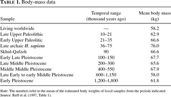
Table 1 lists the estimated body weights for different samples of humans and their respective time ranges.4
The data on living humans to which the fossil body weights are compared refer to a large set of ethnic groups from all over the world; from Irish, to Australian aborigines, to Inuites, to Yemenite Jews (Ruff 1994).

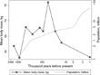
Trends in human body mass and total world population. Sources: for population, Kremer (1993); for body mass, see Table 1. (The times are chosen as the midpoints of the periods reported.)

We are not the first to note this inversely U-shaped pattern, even in the economics literature. For example, the same body mass trends can be seen in Robson and Kaplan (2003, Figure 1), although in a different context (and also is somewhat harder to distinguish because the time scale is not logarithmic). There is also complementary evidence supporting these trends. Ruff (2002, p. 216) points out that many large material artifacts have been found from the periods for which human body mass estimates are relatively big. This suggests that the people who used them were big too.
These changes in body mass also reflect the rise and fall of various human species and changes in geographical habitats. For example, the decline is partly reflected in the extinction of the Neanderthals (late archaic Homo sapiens in Table 1), who were a separate subspecies from modern humans and physically adapted to a colder climate. However, also within our own subspecies, and after the Neanderthals were extinct (i.e., from 35,000 years ago and onward), body mass has declined over time.
In the model set up later, to replicate the rise in human body mass over the earlier phase of human development the population must start off dominated by small body types; this is consistent with the data in Figure 1 and Table 1. One explanation for this initial state of disequilibrium is that prehuman species lived in trees. As for many of our primate relatives today, the bodies of tree dwellers are constrained in size by what tree branches can carry. About two million years ago, as the environment where our ancestors lived became more open and less forested, humanity started to evolve in the form of several new bipedal and terrestrial species. Having just climbed down from the trees, these first humans were thus relatively small. In fact, there was a small initial leap in body mass: the first human species were bigger than their prehuman predecessors. However, the upward trend in body mass also continued among subsequent human species (Ruff 2002, p. 214 and Figure 1).
Population and technology
Whereas body mass has not evolved monotonically, population and technology have. Figure 1 shows the time trend for total world population from 1,000,000 B.C. The numbers are of course not precise but the general trend is not too controversial.
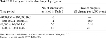
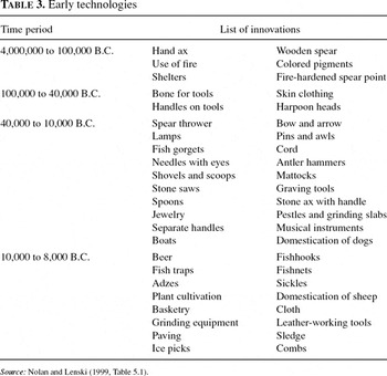
Technology and its growth rate have been increasing over time, at least as measured by the number of innovations per millennium; see Tables 2 and 3. Notably, technological progress also increased before the agricultural revolution, which dates to some time after 10,000 B.C. Also, Table 2 suggests an initial rise in technological progress around 40,000 B.C., about the time body mass began to decline. This coincides with the arrival of anatomically modern humans in Europe, able to produce culture, music, and art, displacing the technologically and culturally backward Neanderthals. This is sometimes referred to as the “Great Leap Forward” (Diamond 1992, Ch. 2).


In the model presented later, technology and population interact in such a way that population growth generates technological progress, or new ideas, and thus further population growth. This relates to a broad literature on scale effects in growth models, going back at least to Kremer (1993); see Jones (2005) for an overview. Such mechanisms may be particularly relevant in the very long-run historical context considered here. For example, many archeologists argue that the invention of agriculture and many preagricultural innovations were driven by rising population pressure and the extinction of large prey (e.g., Smith 1975; Cohen 1977; see Weisdorf 2005 for an overview).
Resource depletion and declining body mass
Resource depletion may also have driven the decline in human body mass. The benefits of having a big body in food procurement are presumably greater in hunting, in particular of large prey (e.g., mammoths), than in gathering food, hunting small prey (e.g., rabbits), or slash-and-burn farming. For example, spears would be easier to use for big individuals; later technologies such as fish gorgets or the bow and arrow (see Table 3) would not require the same physical strength or body mass (Frayer 1981).
At the same time, there are costs of having a big body in terms of greater energy requirements. According to data from FAO/WHO, the maintenance energy required by an adult weighing 65 kg is about 2600 kcal per day; the corresponding requirement for a 10-year-old of 31 kg is 1,750 kcal per day (Payne 1992, Table 3.1). Although there is some debate about the formulas used, these requirements are supposed to give a rough idea of what an individual needs to survive.5
In this example, energy requirements are calculated as 1.5 times the so-called basal metabolism rate (BMR), which in turn is a linear function of age, sex, and body mass. Payne (1992) suggests that energy requirements should rather be calculated as 1.27 times BMR.
This seems to suggest that resource depletion may have shifted the advantage from big to small bodies. Moreover, that such depletion took place is well documented by, among others, Smith (1975) and Diamond (1992, Chs. 17, 18). Examples include extinctions of mammoths, bear-sized beavers, saber-toothed cats, and various species of lion, cheetah, camel, rhino, and horse. The timing seems roughly right too: these extinctions preceded (and perhaps caused) the introduction of agriculture 10,000 B.C.; presumably some prey began to be scarce and harder to find long before that.
It is well known among biologists that large mammals—in particular carnivores, such as humans—tend to be smaller in ecologically isolated environments, most notably on remote islands, known in biology as the “island rule” (Foster 1964).
Similarly to the mechanisms at work in the model presented here, biologists believe that such dwarfism is driven by the limited amount of resources available on islands. When resources are locally depleted on the mainland animals can simply migrate to new areas, but on islands either they become extinct, or only smaller specimens survive (Lomolino 1985).
Many examples of such island dwarfism have been documented among other animals, e.g., elephants (Roth 1992) and three-toed sloths (Anderson and Handley 2002). The evolution of reduced size can also be relatively rapid. Anderson and Handley (2002) document a divergence in skull length of sloths from around 8 cm on the mainland to 7 cm on the island Isla Escudo off the coast of Panama, which was separated from the mainland about 9,000 years ago. The age of first reproduction for sloths is about 3 years; this makes about 3,000 generations. Equally many generations for humans would amount to 60,000 years if each generation corresponds to 20 years. This is the same order of magnitude as the 50,000-year phase of body mass reduction among humans from 80 to 60 kg (cf Table 1).
In fact, it was only recently that a fossil of a previously unknown human species, about 1 m tall when fully-grown, was found on the island Flores in the Indonesian archipelago, thus named Homo floresiensis (Brown et al. 2004; Diamond 2004; Mirazón Lahr and Foley 2004). In a sense, the model presented here can be thought of as an “island dwarfism” story; it explains the decline in human body mass as the result of resource depletion on the larger “island” of planet Earth.
Previous Literature
This paper contributes to a number of recent economic theories on human evolution. Galor and Moav (2001, 2002) study the role of natural selection in shaping quality–quantity preferences for children and are the first to model the interaction between natural selection and the economic environment, as we do here. Others focus on the role played by natural selection in shaping the human mind, e.g., risk preferences and rationality (Robson 2001, 2002, 2003; Galor and Michalopoulos 2006), or model longevity, diseases, and mortality in natural-selection frameworks (Robson and Kaplan 2003; Borghans et al. 2005; Galor and Moav 2005). We abstract from the evolution of preferences and mortality, but may indirectly contribute something to the mentioned theories, because changes in body mass and other physical characteristics could be genetically linked to behavior, preferences, and mortality.6
For example, dogs are smaller and behaviorally different from wolves, from which they were bred (Ridley 2003, pp. 31–37). Also, different from preferences, changes in body structure can be documented and estimated from fossil remains.
Faria (2000) and Horan et al. (2005) analyze the extinction of the relatively large Neanderthals about 35,000 years ago, but not the inversely U-shaped body mass trends explained here. Our story also relates to a literature on resource depletion in preindustrial and preagricultural societies, such as the downfall of the Easter Island civilization (Brander and Taylor 1998; see also Smith 1975, 1992). The idea that resource depletion can lead also to declining body mass arguably makes sense over very long time spans and in a global context, where the “island” is planet Earth rather than Easter Island. It also fits with the so-called island dwarfism phenomenon, as discussed in Section 1.1 above.
Finally, our model relates to many long-run growth models that abstract from natural selection, but do study growth over relatively long time spans of several thousand years (e.g., Galor and Weil 2000; Lagerlöf 2003, 2006).7
THE BASELINE MODEL
Consider an overlapping-generations model where people live for two periods. They are active as adults, and rear passive children. There is only one sex. Agents are heterogenous with respect to body mass. There are G dynasties, and dynasty i has body mass Bi, where

Note that the set of types, B, is exogenous. In other words, there are no mutations involved, and changes in average variables arise only through changes in the composition of the population. Let zi,t denote the fraction of the population with body mass Bi in period t. Average body mass in period t is then given by

A dynasty-i agent active in period t earns an income (or procures an amount of food) given by

where At denotes the level of technology, and Lt is land, or resources, per agent. For simplicity, we treat the resource base as exogenous and normalized to unity, so we can write

where Pt denotes the total (adult) population size in period t. In that sense, rising population and resource depletion here mean the same thing.
It makes sense that income should be increasing in each of its three arguments, holding fixed the other two inputs.8
A large body may be useful when competing for food with other humans; see Section 3.
To generate simple analytical results the following parametric specification is useful,

where η>0 and β>0. That is, technology and body mass are assumed to be perfect substitutes.
Reproductive Success
The reproductive success of an agent of type i is given by his number of (surviving) children, ni,t. This is assumed to depend on resources invested in child rearing, which are given by the difference between the agent's food procurement and his own nutritional needs (his metabolism), which depend on his body mass.
We are going to use the simple functional form

where α>0 denotes the metabolic needs per unit of body mass, Bi, and the product αBi is referred to as subsistence consumption.9
A more precise way to write (6) would be as ni,t=max{0, Yi,t−αBi}. This would serve to explicitly take into account that types whose incomes fall below their subsistence consumption levels become extinct. However, in any period t, fertility will still be given by (6) for all types which are not becoming extinct in that period.

Because both income and subsistence consumption are linear in body mass, so is fertility. Thus, if ∂ni,t/∂Bi>0, big types have more offspring than small types and increase their relative fraction of the population, making average body mass increase from period t to t=1; vice versa, if ∂ni,t/∂Bi<0, small types have more offspring than big types and average body mass decreases. Using (7) it is seen that ∂ni,t/∂Bi>(<)0 whenever Pt<(>)(β/α)1/η. That is, there exists a threshold population level, (β/α)1/η, such that average body mass decreases (increases) over time if population exceeds (falls below) that threshold.
Thus, letting population expand exogenously would shift the reproductive advantage from big to small types and generate the inversely U-shaped trend seen in the data. However, because population evolves endogenously, it remains to see under which restrictions on the parameters this actually happens.
Population
Because fertility is linear in body mass, the average fertility rate takes the same form as in (7), that is,

where we have used (2). Population evolves according to

Technological Progress
The final component of this model is a scale effect on the creation of new technologies. To make the model consistent with technology being fixed in level at early stages of development, technological progress is modelled as a stochastic event. The larger the number of people who can think about new ideas, the more likely is technological progress to occur. More precisely, technology can either be stagnant or progress at some exogenously given rate g>0, and the probability of progress depends on population size, according to

where qt is given by

This particular functional form for qt is chosen arbitrarily but has a reasonable interpretation. The parameter θ is a critical mass of agents needed for technological progress to be feasible; technological progress occurs with positive probability only if Pt>θ. For Pt>θ the probability of technological progress increases with population, and sustained population growth means sustained technological progress at rate g (since
).
Dynamics
To analyze the dynamics in a phase diagram it helps to focus on the case where there are only two body types. In terms of (1), the set of body types can be written as
, where
.
First, consider the phase of development when technology is stagnant, At=A0. Recall from (10) and (11) that this holds with certainty when Pt≤θ, and with positive probability otherwise.
We also assume that A0<β/α. This ensures that, in the technologically stagnant phase, population is greater in the steady state, where big types dominate.
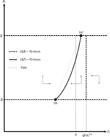
The dynamic behavior of this economy is illustrated in Figure 2 and formalized by the following proposition.

Baseline model dynamics with nongrowing technology.
PROPOSITION 1. Let income be given by (5) and fertility by (6). If there are two body types,
and technology is constant at its initial level A0<β/α, the following holds:
(a) Population evolves according to

(b) Body mass evolves according to the following:
if
or
then ΔBt=Bt=1−Bt=0;
if
then

(c) There are two steady states: one where small types (
) dominate, and one where big types
dominate. The population is larger in the steady state where type
dominates.
The proof is found in the Appendix.
The dynamics are illustrated in the phase diagram in Figure 2. If the economy starts off with a collapsed distribution where the big body type is extinct it converges to the steady state SS, following a path given by the horizontal line
; there is no body mass dynamics.
If the initial fraction of large agents is very small but strictly positive, and the initial population is low, the economy initially tends to gravitate relatively rapidly toward the neighborhood of SS, before converging to SS′. The reason is that as long as the economy is situated far from the (ΔPt=0)-locus, and close to the (ΔBt=0)-locus, population adjusts relatively rapidly and body mass more slowly. It is thus natural to consider SS as the starting point of human history two million years ago, just after humans had become bipedal.
An economy starting off close to SS stays there for a long time and eventually follows a trajectory close to the (ΔPt=0)-locus, with expanding population and growing average body mass, approaching SS′. The steady state SS′ has larger population than SS given that A0<β/α. The trajectory is illustrated by the dotted path in Figure 2.
Population is larger at SS′ than at SS because, in technologically backward (and thus sparsely populated) environments, body mass is an important input in food procurement and big types thus rear more offspring. In a sense, a rise in average body mass affects steady state population in a manner similar to a (small) rise in technology: as agents become bigger they can procure more food and thus sustain a larger population. Put differently, when converging from SS to SS′ population grows as a result of increasing average body mass: aggregate population expands because the composition of the population shifts toward big types who have higher reproductive rates.
Average body mass stops growing when the biggest type dominates because the set of body types is assumed to be fixed. If instead mutations bigger than
enter the population over time average body mass can increase indefinitely (cf. the discussion of Cope's rule in Section 3 later). Similarly, if small types have the reproductive advantage, mutations smaller than
can diminish average body mass indefinitely.
In a two-type setting and absent the possibility of technological progress the economy stays forever at SS′ in Figure 2, where big types dominate and the population is nongrowing. Something akin to this may have happened to many nonhuman species that never began to develop new technologies (at least not to the same extent as humans). Gorillas could be one primate example.
Now allow for technological progress. Recall from (10) and (11) that as population reaches the threshold θ, technological progress occurs with positive probability. Once a rise in technology has occurred the feedback loop between population and technological progress sets in. In terms of Figure 2 it would imply that population expands throughout the whole range of Pt considered. [The dynamics of body mass do not depend directly on technology, so the (ΔBt=0)-locus is unchanged.] As population comes to exceed (α/β)1/η the reproductive advantage shifts to small types and average body mass starts to decline, approaching
.
Moreover, the decline in body mass is faster than the preceding rise, because the trajectory it follows is situated farther from the (ΔBt=0)-locus.
Letting Pt go to infinity and Bt go to
in (8) or (9) one can deduce the following.
PROPOSITION 2. Let income be given by (5) and fertility by (6). If there are two body types,
and technology grows at rate g, then the economy converges to a balanced growth path where
, and population grows at rate (1=g)1/η−1.
The proof is in the Appendix.
This balanced growth path should not be thought of as describing the modern economy in which we live today, but rather the state of slow but positive technological progress prevailing in the preagricultural phase of development before 10,000 B.C. (see Tables 2 and 3).
A COMPETITION MODEL
The baseline setting presented so far is one of the most intuitive and transparent models that can replicate the trends described earlier. Many assumptions can be relaxed without changing the underlying mechanics and results. For example, having a big body may be an advantage in competing with other humans for food. If so, not only absolute body mass, Bi, may affect food procurement, but also relative body mass, Bi/Bt.
Consider the extreme case where only relative body mass matters, and absolute body mass plays no role at all. Analogously to the specification in (5), let

With this formulation there is no net food gain as the average agent grows bigger; the average agent procures
independent of Bt. Using the expression for fertility in (6), ni,t=Yi,t−αBi, it can then be seen that

As in the baseline model, the sign of ∂ni,t/∂Bi determines which type (big or small) has the reproductive advantage and increases its share of the population. From (15) it thus follows that body mass decreases (increases) over time if
.
Holding constant the level of technology at some level A, the dynamics of Bt and Pt can be analyzed in a two-dimensional phase diagram. First consider a formal characterization of the dynamics.
PROPOSITION 3. Let fertility be given by (6) and income by (14). If there are two body types,
and technology is constant at some level A, the following holds:
(a) Population evolves according to

(b) Body mass evolves according to the following:
if
or
then ΔBt=Bt=1−Bt=0;
if
then

(c) For all levels of technology two steady states exist, where either small types
or big types
dominate; the population is smaller in the steady state where
dominates.
(d) For intermediate levels of technology,
there also exists a steady state where body mass equals
and population equals P=A1/η.
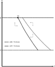
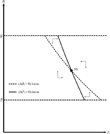
The proof is found in the Appendix. Figure 3 illustrates the dynamics for the case with a low level of technology,
, and Figure 4 the case with intermediate technology,
.

Competition model dynamics with low technology.

Competition model dynamics with intermediate-level technology.
The point SS in Figure 3 is a stable steady-state equilibrium with small population and large average body mass. It can be seen from (15) that an (exogenous) rise in technology has no direct effect on the sign of ∂ni,t/∂Bi, thus leaving the (ΔBt=0)-locus unchanged. However, an increase in technology raises the fertility of all agents and thus makes the (ΔPt=0)-locus shift out, pushing the steady state towards smaller bodies and larger populations; see point SS in Figure 4.
As in the baseline setting, one can allow for a scale effect in technology production, as in (10) and (11). This would make an initial rise in technology generate an expansion in population, thus spurring more technological progress, and so on. The result is a chain process by which the (ΔPt=0)-locus shifts out at an increasingly rapid rate, pushing the steady state down along the (ΔBt=0)-locus (cf. Figure 4). In that sense, a competition model can indeed replicate a pattern of declining body mass in parallel with explosive growth in population and technology, just as in the baseline setting and in the data (see Figure 1).
However, the competition model does not fully replicate the type of gradual and simultaneous rise in population and body mass that characterized the earlier phase of human evolution in Figure 1. In the baseline model the economy followed a path of slow and gradual increases in population because the path stayed close to the (ΔPt=0)-locus (cf. Figure 2). Here, however, a path close to the (ΔPt=0)-locus displays rising body mass and falling population. Intuitively, there is no net food gain as the average agent grows bigger, only higher metabolic costs. Therefore greater average body mass leads to lower average fertility and thus to smaller steady state population. (If the economy instead started off close to
and Pt=0 it would display an initially too rapid rate of population growth.)
However, a (perhaps more realistic) model where body mass affects food procurement in both absolute and relative terms can in principle generate the same gradual and simultaneous rise in population and body mass as seen in the baseline model.
Nonhuman Species and Cope's Rule
Interestingly, the simultaneous rise in body mass and decline in population in this type of competition model may be relevant to other species and eras. Valkenburgh et al. (2004) document how over the past 50 million years many carnivorous animal species native to North America displayed increasing body mass prior to becoming extinct. Similar to the mechanics of the competition model presented in this section, their explanation is that selection for large bodies was driven by the competitive advantage of larger size, known as Cope's rule. Given that energy requirements are greater for bigger agents this can lead to declining population of the whole species, and even its extinction. In other words, natural selection can promote bigger bodies because it is associated with higher reproductive success of the individual agent, but it may nevertheless result in population decline (and eventual extinction) of the whole species.
Technology as Input in Competition
An alternative competition model is one where both technology and body mass are used in competition. As an extension of (14), let

for some γ≥0; setting γ=0 brings us back to (14). Note that technology is not only an input in competition; there is also (as before) a direct food gain from technological progress, because the average agent procures
(but there is no food gain for the average agent as average body mass increases).
With this formulation, technological progress functions as an equalizing force in competition, because it reduces the excess amount of food procured by big types. Compared to the production function in (14), the implication in terms of the phase diagrams in Figures 3 and 4 is that increases in technology here lead to an inward shift of the (ΔBt=0)-locus. (To see this, use (18) and (6) and note that ∂ni,t/∂Bi is decreasing in At.) The qualitative predictions are thus the same as in the previous competition model: rising technology leads to expanding population and declining body mass. The difference is that technological progress here directly drives the decline in body mass by lowering the competitive value of a big body.
CONCLUSIONS
We have presented a model of endogenous growth in population and technology, together with natural selection among body types. The model can explain why humans were becoming bigger up until 50,000 years ago, and since then have been declining in size. The central mechanism driving these results is that technological progress does not in itself affect the relative reproductive advantage of big and small types, but it does bring with it denser population and depletion of resources and thereby shifts the reproductive advantage to smaller body types.
This story is not meant to be an exhaustive explanation of human physiological history but may serve as a starting point for thinking about related mechanisms at work between the same variables. For example, it seems that changes in body mass over time reflect changes in human habitats. The fossils of the largest humans over the past two million years have been found predominantly (but not only) in colder regions (Ruff 2002). The reason is that heat saving becomes more important in colder climates, which works better with bigger bodies and more “cubic” forms, i.e., larger trunks and shorter limb segments, known as Allen's and Bergmann's rules, respectively.10
Think of the human body as a cube with side x, so that its volume equals x3 and its surface 6x; the volume-to-surface ratio is thus given by x/6. The higher is this ratio the lower is the heat loss, so larger bodies (with higher x) are more beneficial in cold climates. This is Allen's rule. Likewise, if the body is a rectangle of fixed volume, V, and variable sides x, y, and z, then it can be seen that the volume-to-surface ratio is maximized when x=y=z=V1/3, that is, when the rectangle is a cube. This is Bergmann's rule. See Jurmain et al. (2000, pp. 423–426) for a textbook overview.
Body mass may also have declined as a way to rapidly increase the brain-to-body (encephalization) ratio and thus intelligence (Kappelman 1996, 1997; Robson and Kaplan 2003). Up until about 50,000 years ago encephalization had increased as brains and bodies expanded in tandem. One may conjecture that selective pressures for intelligence then increased, due to denser populations making cooperation more important, more advanced technologies being developed, and/or language evolving around this time (Diamond 1992). This could have increased the reproductive value of high encephalization, but it is not clear why rising encephalization would come with declining body mass only over the last phase of development. Also, the examples of island dwarfism among other species (cf. Section 1.1) suggest that declining body mass can occur also without the development of humanlike levels of intelligence.
Other issues relating to historical body trends could be interesting to study in future work. As suggested by Diamond (2003), over recent centuries natural selection may have reduced the prevalence of fat-storing “thrifty genes,” which improve the chance of surviving starvation, but also make the carrier more susceptible to obesity and diabetes. Geographical variation in the timing of improved food supply may therefore explain variation in such conditions today.
APPENDIX
A.1. THE BASELINE MODEL
Proof of Proposition 1
(a) The (ΔPt=0)-locus. Consider first the segment of the phase diagram where
; this in turn implies that Pt <(β/α)1/η (because A0 < β/α). The former of these two inequalities implies that
; the latter implies that
(because Bt>0). From (9) this is seen to imply that Pt=1 > Pt; thus population is always growing when
.
Consider next the segment of the phase diagram where
. Using (9) we see that Pt=1>reqqlessPt holds when
, which is (12). The (ΔPt=0)-locus in Figure 2 is given by (12) holding with equality.
Consider next the segment of the phase diagram where (β/α)1/η<Pt<([β=A0/Bt]/α)1/η. These inequalities imply that
, and
, so using (9) it is seen that Pt=1<Pt; thus population is decreasing in this region of the phase diagram.
Note, for completeness, that Pt>([β=A0/Bt]/α)1/η would imply negative fertility (or fertility being constrained to zero) and thus the population becoming extinct.
(b) The (ΔBt=0)-locus. When all agents belong to the same body type the composition cannot change. When there are only two body types,
and
, Bt must thus be constant whenever either body type dominates the population, that is, when
or
. Average body mass is increasing (decreasing, constant) when ∂ni,t/∂Bi>(<, =)0. Using (7), this amounts to
, which gives (13).
(c) From (12) and (13) it is seen that the denominator of (13) is zero if ΔBt=0 for
. Thus, the only steady states that can exist must be such that
or
. These steady states do exist because ΔPt=ΔBt=0 at
, where
, and
, where
. Because
, and [(A0=βB)/(1=αB)]1/η is increasing in B for A0<β/α, it must hold that
. Q.E.D.
Proof of Proposition 2
Use (9) to see that if Pt grows at a sustained constant rate, and thus Bt approaches
, then fertility (and thus population growth) approaches
. For this growth rate to be constant,
must be constant. Because At=1=(1=g)At it follows that
, or Pt=1=(1=g)1/ηPt; this gives
. Q.E.D.
A.2. A COMPETITION MODEL
Proof of Proposition 3
(a) The (ΔPt=0)-locus. Treating technology, A, as fixed, and using Pt=1=Ptnt, (2) and (15), it is seen that

Setting Pt=1=Pt in (19) we get
, which is (16). Likewise, when
it is seen from (19) that Pt=1<(>)Pt.
(b) The (ΔBt=0)-locus. As in the proof of Proposition 1, we note that Bt=1=Bt when one single type dominates the whole population (so that, in the two-type case,
or
). Otherwise, Bt=1>(<, =)Bt when ∂ni,t/∂Bi>(<, =)0. Using (15), this gives (17).
(c) From (16) and (17), it is seen that ΔPt=ΔBt=0 when
, where
, and
, where
. Since
, and [(A=β)/(1=αB)]1/η is decreasing B, it must hold that
.
(d) If a steady state where
exists, then (16) and (17) say that both
and
must hold. Solving for Bt and Pt gives Pt=A1/η and Bt=β/(αA); and
is equivalent to
. Q.E.D.
I am grateful for comments from Omer Moav, Steeve Mongrain, Arthur Robson, Abhijit Sengupta, seminar participants at York University and Simon Fraser University, two anonymous referees, and an associate editor. Financial support from the Social Sciences and Humanities Research Council of Canada is gratefully acknowledged. All errors are mine.