INTRODUCTION
Optimal maize production depends on genotype (G), environment (E) and both together when there is significant G × E interaction (Allard Reference Allard1999). Efforts have been made to quantify, minimize or make use of the G × E interaction when making strategic decisions regarding maize breeding (Cruz et al. Reference Cruz, Regazzi and Carneiro2006).
The additive main effects and multiplicative interaction (AMMI) models developed by Kempton (Reference Kempton1984); Gauch & Zobel (Reference Gauch and Zobel1988); Zobel et al. (Reference Zobel, Wright and Gauch1988) and Crossa et al. (Reference Crossa, Fox, Pfeiffer, Rajaram and Gauch1991) are important statistical methods for plant breeding. Although these models provide easy and simple methods for interpreting parametric estimators, they require normally distributed data.
Kempton (Reference Kempton1984) discusses the method of principal components (PC) as a way to summarize the response of a genotype to different environments. In this method, the matrix of estimated G × E interaction effects from the classical analysis of variance (ANOVA) model is subjected to principal component analysis (PCA). The G × E interaction is thus decomposed into a number of multiplicative terms. The hypothesis is that most of the G × E interaction can be explained by the first few terms of the PCA and that these have some meaningful interpretations.
The AMMI model has been applied since the 1990s to evaluate G × E interactions and allow breeders to recommend stable cultivars adapted to either broad or specific environments. However, the AMMI model can only be applied when the response variable Y follows a normal distribution with a homogeneous variance. If these assumptions are not met, a methodology based on a generalized linear model (GLM) is more appropriate. Algorithms for generalized additive main effects and multiplicative interaction (GAMMI) developed by van Eeuwijk (Reference van Eeuwijk1995) and Gabriel (Reference Gabriel1998) are based on the basic concepts for AMMI expanded by the theories of GLM and the quasi-likelihood method. These GAMMI models assume that the response variables have an exponential probability distribution. Earlier, Wedderburn (Reference Wedderburn1974) established the quasi-likelihood method to accommodate a wider range of possible distributions and variances (Agresti Reference Agresti2002). The quasi-likelihood method is a generalization of the GLM (Paula Reference Paula2004) that assumes a single relationship between the mean and variance rather than an a priori distribution for Y. Similar to the GLM, the quasi-likelihood model assumes a link function that is a linear predictor instead of a specific distribution of the response variable Y (McCullagh & Nelder Reference McCullagh and Nelder1989). It also assumes that Var(Y) = φ Var(μ), where μ is the mean of Y, V(μ) is a new function of μ and φ is the dispersion parameter.
Grey leaf spot can severely affect susceptible cultivars, resulting in crop losses of greater than 0·80. In maize, the symptoms of grey leaf spot include irregular, rectangular grey spots that develop parallel to the leaf veins (Fantin et al. Reference Fantin, Brunelli, Resende and Duarte2001; Fornasieri Filho Reference Fornasieri Filho2007). According to Brito et al. (Reference Brito, Von Pinho, Pozza, Pereira and Faria Filho2007), the pathogen colonizes large areas of foliar tissue, reduces photosynthesis, induces early leaf senescence and decreases crop yield. Wind or raindrops can disseminate the pathogen. Because the spores remain on the stover after harvest, a management strategy must be adopted to reduce recontamination (Bhatia & Munkvold Reference Bhatia and Munkvold2002).
Thus, a maize variety carrying a large number of resistance genes is likely to have better yield in environments in which grey leaf spot is prevalent. Such genotypes must have stable, high yield with little variation in different environments (Tarakanovas & Ruzgas Reference Tarakanovas and Ruzgas2006).
The objective of the present study was to evaluate and quantify the G × E interaction for response to grey leaf spot in maize using GAMMI models to identify genotypes that are resistant to grey leaf spot, adapted to specific environments, or both.
MATERIALS AND METHODS
Data pertaining to grey leaf spot severity in Brazil were collected from 36 maize cultivars evaluated in nine different environments in 2010/11. The experimental design in each environment was a randomized complete block with two replications. Plots consisted of four 5-m rows spaced 0·70 m apart with experimental units of 14 m2. Fertilization, liming and other cultural practices were applied as required in each location and experimental area. Grey leaf spot severity was quantified as the percentage of diseased leaf area within each plot.
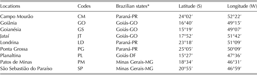
The locations in which the 36 genotypes (G1 to G36) were evaluated by EMBRAPA are shown in Table 1. In the first stage of the present study, the Shapiro–Wilk multivariate normality test and the Bartlett test for homogeneity of variance were used to determine whether to apply an AMMI model or a GAMMI model to analyse the G × E interactions for incidence and severity of grey leaf spot in maize in these environments.
Codes and geographic coordinates for the locations in which maize genotypes were evaluated

* State name and state abbreviation.
Additive main effects and multiplicative interaction model
The AMMI model was composed of additive and multiplicative components where Y represents a vector of n independently distributed observations that can be predicted by the categorical variables for genotypes and environments. The additive component, with fixed main effects for genotype (α i ) and environment (β j ), was assumed to be a fixed effect, and inferences were restricted to the grey leaf spot response variables, disease incidence and severity (Searle et al. Reference Searle, Casella and McCulloch1992).
A least-squares method was used to estimate these effects via a two-way ANOVA using the means matrix for Y
(gxe). The multiplicative component was estimated by the singular value decomposition (SVD) of the residual matrix from the two-way ANOVA of the genotype–environment means Y
(gxe). This matrix will be denoted as R
(gxe). Generally, the SVD of a matrix A is defined as the product of an orthogonal matrix U by a diagonal matrix S and the transpose of the orthogonal matrix V; thus,
 $A_{mn} = U_{mn} S_{mn} V_{nn}^T $
. Required conditions are that UTU = I and VTV = I; the columns of U are orthonormal eigenvectors of AAT
; the columns of V are orthonormal eigenvectors of ATA; S is a diagonal matrix containing the square roots of eigenvalues from U or V in descending order; and A = VS2VT
(Ientilucci Reference Ientilucci2003).
Therefore, the model equation for the ith genotype in the jth environment in the rth block is (Gauch & Zobel Reference Gauch and Zobel1988):
 $$Y_{ijr} = \underbrace {\mu + \alpha _i + \beta _j + \rho _{r(\,j)}} _{additive\; terms} + \underbrace {\sum\limits_{h = 1}^p {\lambda _h \gamma _{ih} \delta _{\,jh}}} _{multiplicative\; terms} + \,\varepsilon _{ijr} $$
where Y
ijr
is the phenotypic trait (i.e., the proportion of plants affected by grey leaf spot) of genotype i in environment j for replicate r; μ is the grand mean; α
i
is the fixed effect for genotype i, where i = 1, 2, …, g; β
j
is the fixed effect for the environment j, where
 $j = {\rm 1},{\rm 2},..., e;\,\lambda _h $
is the singular value for the interaction principal component (IPC) axis k; γ
ih
and δ
jh
are the IPC scores (i.e., the left and right singular vectors) for genotype and environment, respectively, for axis k; ρ
r(j) is the effect of the rth block in the jth environment; r is the number of blocks; p is the rank of the R
(gxe) matrix that corresponds to the number of main effects from the interaction (PCI) retained by the residual matrix,
 $p\,{\rm =} \,min{\rm (}{\rm g}{\rm - 1}{\rm,} \;{\rm e}{\rm - 1)};\ {\rm (}\alpha \beta {\rm )}_{ij} = \sum\nolimits_{h = {\rm 1}}^p {\lambda _h \gamma _{ih} \delta _{jh}} $
is the specific interaction of the ith genotype with the jth environment and ε
ijr
is the experimental error that is assumed to be independently and normally distributed with a mean of zero and variance
 $\sigma ^2, \;\varepsilon _{ijr} \sim N(0,{\rm \;} \sigma ^2 ){\rm.} $
The decomposition of the residual matrix into singular values (SVD) permits the partitioning of the least squares from the elements of the R
(gxe) matrix by reducing the number of axes, or K < p such that the model remains informative, where K is the number of axes or PC retained by the model, but with fewer degrees of freedom. This partition is:
 $$\mathop \sum \limits_{h = 1}^p \lambda _h \gamma _{ih} \delta _{\,jh} = \mathop \sum \limits_{h = 1}^K \lambda _h \gamma _{ih} \delta _{\,jh} + \mathop \sum \limits_{h = 1 + K}^p \lambda _h \gamma _{ih} \delta _{\,jh}, $$
where
 $\sum\nolimits_{h = 1 + K}^p {\lambda _h \gamma _{ih} \delta _{jh} = \varphi _{ijr}} $
quantifies the disturbance and ϕ
ijr
is the residual containing all of the multiplicative terms not included in the model.
Therefore, using the least-squares approximation to the R (gxe) matrix by the first n components of the SVD, the reduced model ηijr is estimated by:
 $$\hat Y_{ijr} = \underbrace {\hat \mu + \hat \alpha _i + \hat \beta _j + \hat \rho _{r(\,j)}} _{additive\; terms} + \underbrace {\sum\limits_{h = 1}^K {\lambda _h \gamma _{ih} \delta _{\,jh}}} _{multiplicative\; terms}$$
The PCA permits the components from the interaction to capture the decreasing proportion of the variation that is present in matrix GE, or
 $\lambda _{\rm 1}^{\rm 2} \ge \lambda _{\rm 2}^{\rm 2} \ge {\cdots} \ge \lambda _K^{\rm 2} $
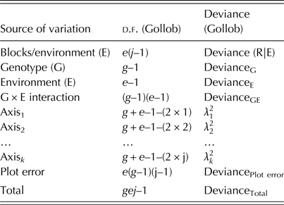
. A sufficient number of components (K) to represent the target model can be identified using Gollob's test (Table 2) (Gollob Reference Gollob1968).
Complete variance analyses of the means according to Gollob (Reference Gollob 1968 )

Generalized linear models
When a distribution is non-normal, GLMs expand the possibilities for statistical modelling. These models allow fitting of n random variables y i , where i = 1, 2,…, n, that are independently distributed with mean μ i and an exponential probability density function. These random variables are associated with the explanatory variables x j, j = 1, 2, …, p by means of a link function g(μ i ) designated as the linear predictor (η i ) that is monotonic and differentiable such that:
 $$\eta _{\rm i} = g{\rm (}\mu _i {\rm )} = \sum\limits_{{\rm j} = {\rm 1}}^{\rm p} {x_{{\rm ij}} \psi _{\rm j}} $$
where ψ j represents the coefficients of the linear predictor.
The maximum-likelihood method is the most useful method for estimating the vector of the unknown parameters of the linear predictor ψ j . Cordeiro & Demétrio (Reference Cordeiro and Demétrio2008) explained that the robust and fast GLM algorithm rarely fails to converge. However, when this does happen, the fitting procedure must be restarted using the current estimate as the starting value for another model.
The deviance function derived from the likelihood ratio statistic tests the significance of the coefficients of the linear predictor. Therefore, in a sequence of k nested models (which have the same probability distribution and link function, but the linear component M 0 is a special case of the general linear component M 1) (Dobson Reference Dobson2002), tests of significance are performed using an analysis of deviance (ANODEV) table. Thus the deviance function from the GLMs is analogous to the residual squared sums from least squares. Standardized Pearson residuals, standardized deviance residuals, and Cook's distance measures were used to diagnoses in the quasi-likelihood models.
Quasi-likelihood models
Quasi-likelihood has been used due to the characteristics of the data and the model. Although the GLM represents a great advance in statistical modelling because it allows the fitting of a large number of models, in some instances the choice of an exponential model is not adequate (McCullagh & Nelder Reference McCullagh and Nelder1989), so Wedderburn (Reference Wedderburn1974) proposed quasi-likelihood estimation. Assuming that Var(μ) is a known function of the mean, and φ is the dispersion parameter, the quasi-likelihood function for every observation is
 $$Q_i = Q_i (y;\mu ) = \mathop{\int}\limits_{y_i}^{\mu _i} {\displaystyle{{y_i - t} \over {\phi {\cdot} Var{\rm (}t{\rm )}}}dt} {\rm,} \quad y_i \le t \le \mu _i $$
Inference in quasi-likelihood models is similar to that in GLM because quasi-likelihood estimates maximize Q or solve the following system of equations:
 $$\sum\limits_{i = 1}^n {\displaystyle{{{\rm (}y_i - \mu _i {\rm )}} \over {\phi V{\rm (}\mu _i {\rm )}}}} \displaystyle{{\partial \mu _i} \over {\partial \psi _j}} = 0{\rm,} \;\,j = 1{\rm,} \ldots {\rm,} p$$
and
 $$\sum\limits_{i = 1}^n {\displaystyle{{{\rm (}y_i - \mu _i {\rm )}x_{ij}} \over {\phi V{\rm (}\mu _i {\rm )}}}} \displaystyle{{\partial \mu _i} \over {\partial \eta _i}} = 0$$
In the first system,
 $\mu _i = g^{ - 1} {\rm (}\eta _i {\rm )} = g^{ - 1} {\rm (}z_i^T \psi _j {\rm )} = h{\rm (}x_i^T \psi _j {\rm )}$
and this expression are based on the GLM theory. The dispersion φ is estimated using the method of moments on the residual vector
 ${\rm (}Y - \hat \mu {\rm )}$
:
 $$\hat \phi = \displaystyle{1 \over {n - p}}\sum\limits_{i = 1}^n {\displaystyle{{{\rm (}y_i - \hat \mu _i {\rm )}^2} \over {V{\rm (}\hat \mu _i {\rm )}}}} = \displaystyle{{\chi ^2} \over {n - p}}$$
where χ 2 is Pearson's generalized chi-square statistic for goodness-of-fit, n is the number of observations, and p is the number of parameters (ψ j ). The generalized function can be estimated in a similar manner to the deviance function, using the difference between the quasi-likelihood logarithm of the current and the saturated models:
 $$\eqalign{D{\rm (}y{\rm ;}\hat \mu {\rm )} = & 2\phi {\rm \{} Q{\rm (}y{\rm ;}y{\rm )} - Q{\rm (}\hat \mu {\rm ;}y{\rm )\}} \cr = & - 2\phi {\rm \{} Q{\rm (}\hat \mu {\rm ;}y{\rm )} - Q{\rm (}y{\rm ;}y{\rm )\}}} $$
Because the contribution from the saturated model is zero, then:
 $$\eqalign{D{\rm (}y{\rm ;}\hat \mu {\rm )} & = - 2\phi Q = - 2\phi \sum {\mathop\int\limits_{y_i} ^{\mu _i} {\displaystyle{{y_i - t} \over {\phi V{\rm (}t{\rm )}}}}} dt \cr & = - 2\sum {\mathop\int\limits_{y_i} ^{\mu _i} {\displaystyle{{y_i - t} \over {V{\rm (}t{\rm )}}}}} dt}$$
Thus, the quasi-deviance function does not depend on the dispersion parameter φ. The quasi-deviance function
 $D{\rm (}y{\rm ;}\hat \mu {\rm )}/\phi $
is compared with the percentiles of the χ
2 distribution with (n–p) degrees of freedom, although the null distribution of
 $\phi ^{ - 1} D{\rm (}y{\rm ;}\hat \mu {\rm )}$
is not usually known (Paula Reference Paula2004).
Generalized additive main effects and multiplicative interaction
The GAMMI theory requires the same basic assumptions as the GLMs. The response variable Y must be independently distributed and have a known exponential family distribution, and p associated explanatory variables X j, where j = 1, 2, …, p are determined by a link function g(μ i ) that designates a linear predictor η i that is monotonic and differentiable such that:
 $$\eta _i = g(\mu _i ) = \mathop \sum \limits_{\,j = 1}^p X_{ij} \psi _j $$
These linear predictors have been useful to estimate the mean severity of grey leaf spot. Because the link function was the logit in which η = g(μ) = log(μ/1 − μ), the mean proportion of disease was estimated by the relationship
 $$g^{ - 1} (\eta _{ijr} ) = \displaystyle{{exp(\mu + \alpha _i + \beta _j + \rho _{r(\,j)} + \sum\limits_{h = 1}^K {\lambda _h \gamma _{ih} \delta _{\,jh} )}} \over {1 + exp(\mu + \alpha _i + \beta _j + \rho _{r(\,j)} + \sum\limits_{h = 1}^K {\lambda _h \gamma _{ih} \delta _{\,jh} )}}} $$
where K is the number of axes considered.
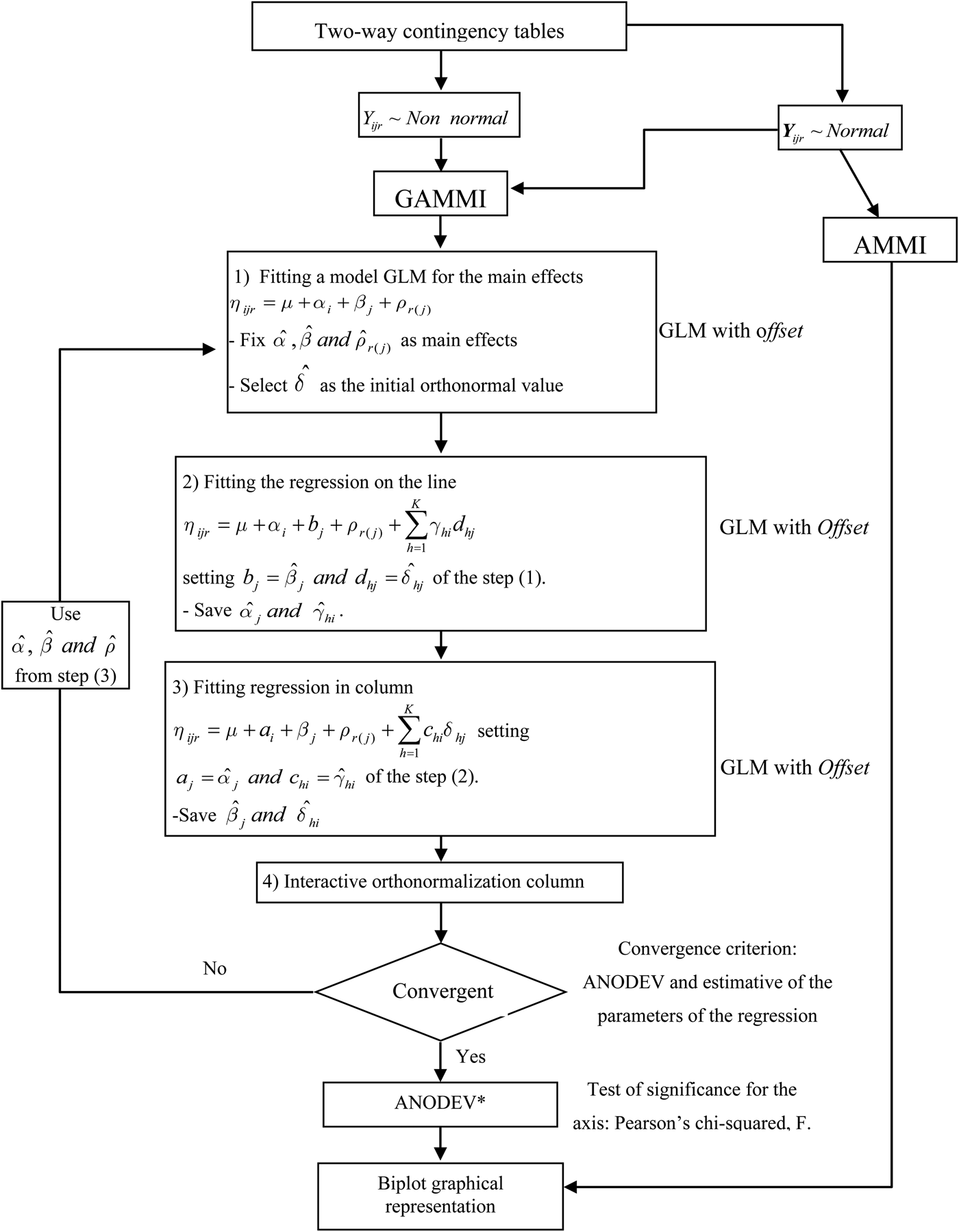
The GAMMI model is applied using van Eeuwijk's algorithm adapted from Sumertajaya (Reference Sumertajaya2007) in R software version 3.0·2 (R Development Core Team 2013) using the R package gnm (generalized nonlinear models) (Turner & Firth Reference Turner and Firth2009). This algorithm uses iterative alternating generalized regression of rows and columns to estimate the parameters. The first step in determining the appropriate model is to identify the distribution and handling of the experimental data. An error plot should be used to visualize whether the data have, for example, a Poisson or binomial distribution instead of a normal distribution. The second step is to fit the GAMMI model, in which each regression includes a GLM class that is arrived at iteratively. This algorithm involves convergence in row regression, in column regression, and in alternating regression (Hadi et al. Reference Hadi, Mattjik and Sumertajaya2010). If the model converges, then ANODEV may then be performed. Finally, the data matrix is represented as a biplot. Figure 1 shows the algorithm necessary for applying the GAMMI model.
van Eeuwijk's algorithm for modelling GAMMI, adapted from Sumertajaya (Reference Sumertajaya2007). *Analysis of Deviance (ANODEV).

To determine the number of axes or the number of multiplicative terms in a GAMMI model, a generalization of the AMMI method via the tests described below may be used. The F test does not require a special table and is easy to calculate. The statistic used is F = (Dev. restricted/D.F. sv restricted)−
 $({\rm Dev}{\rm. \; full}/ {\rm D}{\rm. F}{\rm. \; full})/\hat \phi $
, which approximates the F(D.F.source of variation; D.F.error) distribution. Where:
 ${\rm Dev}{\rm. :deviance},\,\hat \phi $
is the dispersion parameter from quasi-likelihood estimation, D.F..sv: degrees of freedom from source of variation that is being tested.
The test proposed by Gollob (Reference Gollob1968) allocates (g − 1)(e − 1) − (2k − 1) = g + e − 1 − 2k degrees of freedom to the eigenvalues associated with the kth axis, where k = 1, 2,…, n and n = minimum (g–1, e–1), which corresponds to the difference between the number of parameters to be estimated and the number of factors applied. Thus, the mean deviance is tested against the estimated error.
Stability is the maintenance or predictability of the response variable in various environments (Annicchiarico et al. Reference Annicchiarico, Bellah and Chiari2005; Cruz et al. Reference Cruz, Regazzi and Carneiro2006). For the incidence or severity of disease, a genotype is considered to be stable when its disease severity percentage is low and constant with respect to environmental variation under both specific and broad conditions. Stability is estimated by analysing the magnitude and sign of the biplot scores corresponding to the selected GAMMI model. Genotypes and environments with low (near zero) scores are considered stable, which is expected for genotypes and environments that have a small contribution to the overall interaction (Duarte & Vencovsky Reference Duarte and Vencovsky1999).
The adaptability of a genotype indicates its ability to take advantage of environmental effects to ensure a high level of productivity. Adaptability is predicted as a function of the responses for each combination of genotype and environment in the model selected by GAMMI IPCAk (axis k: axis of interaction PCA). The correlation between cultivars and the environment is based on the angles between vectors determined by coordinates of the interaction (axis 1, axis 2) and the vertex. The cosine of the two vectors indicates the level of correlation between two corresponding variables (Rencher Reference Rencher2002). Therefore, a small angle indicates highly positively correlated variables, perpendicular vectors indicate non-correlated variables, and an angle greater than 90° indicates a negative correlation.
RESULTS
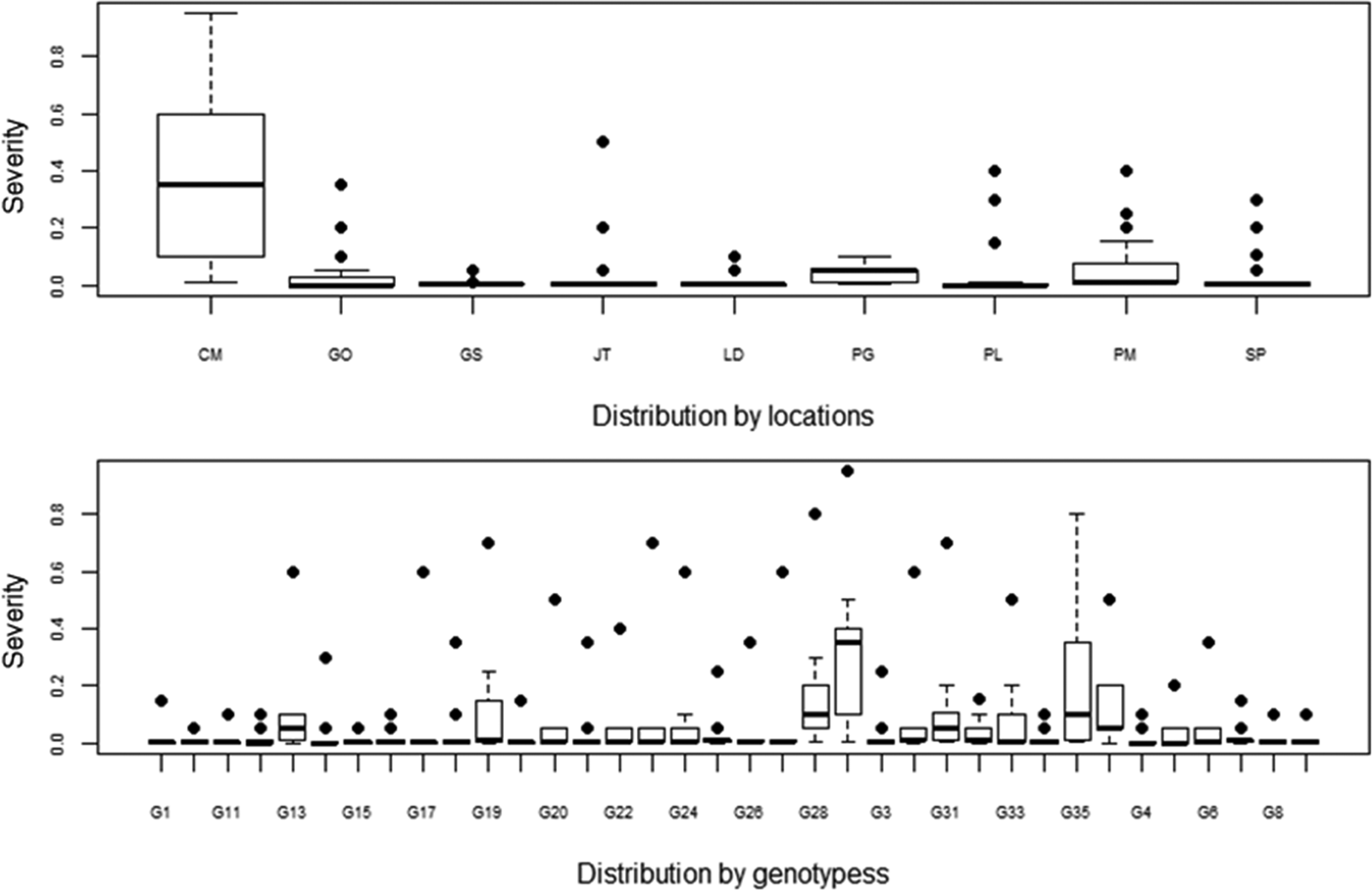
Box plots of grey leaf spot incidence showed strong evidence of asymmetric disease severity and discrepancies in the data for the distribution of disease by location and genotype (Fig. 2).
Box plot of environments and genotypes showing the distribution of grey leaf spot severity. Locations: Campo Mourão (CM), Goiânia (GO), Goianésia (GS), Jataí (JT), Londrina (LD), Ponta Grossa (PG), Planaltina (PL), Patos de Minas (PM) and São Sebastião do Paraíso (SP).

The results of the Shapiro–Wilk test (W) indicated that the data were not normally distributed (W = 0·4974, P < 2·2 × 10−16). Similarly, the hypothesis of homogeneous variance was rejected based on results of the Bartlett test, both for genotype (d.f. = 35; χ 2 = 520·30; P < 2·2 × 10−16) and location (d.f. = 8; χ 2 = 682·88; P < 2·2 × 10−16).
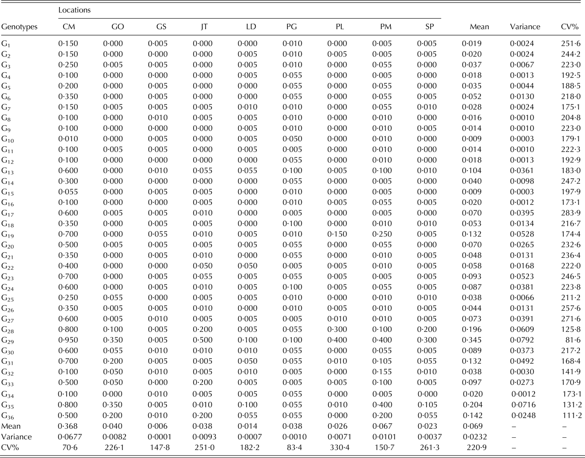
Thereafter, the first step in applying the GAMMI methodology was to determine the means, variances and coefficients of variation (CV) for the severity of grey leaf spot. Some discrepant values for location and genotype were detected. The highest disease severity levels were detected in Campo Mourão (36·85%) and Patos de Minas (6·67%), and the lowest levels were detected in Goianésia (0·61%) and Londrina (1·45%). Campo Mourão had the lowest coefficient of variation (70·6%) for disease severity, while those for Planaltina (329·5%) and São Sebastião do Paraíso (260·9%) were very high. Coefficient of variation values for other locations ranged from 83·4 to 250·7%. Moreover, there was large variability in disease severity among genotypes. Means for grey leaf spot severity ranged from 0·9 (G15 and G10) to 34·5% (G29) and the CV values ranged from 81·6 to 283·9% (Table 3).
Mean values of grey leaf spot severity estimated from two replications of 36 maize cultivars grown in nine locations during the 2010/11 growing season

CM, Campo Mourão; GO, Goiânia; GS, Goianésia; JT, Jataí; LD, Londrina; PG, Ponta Grossa; PL, Planaltina; PM, Patos de Minas; SP, São Sebastião do Paraíso.
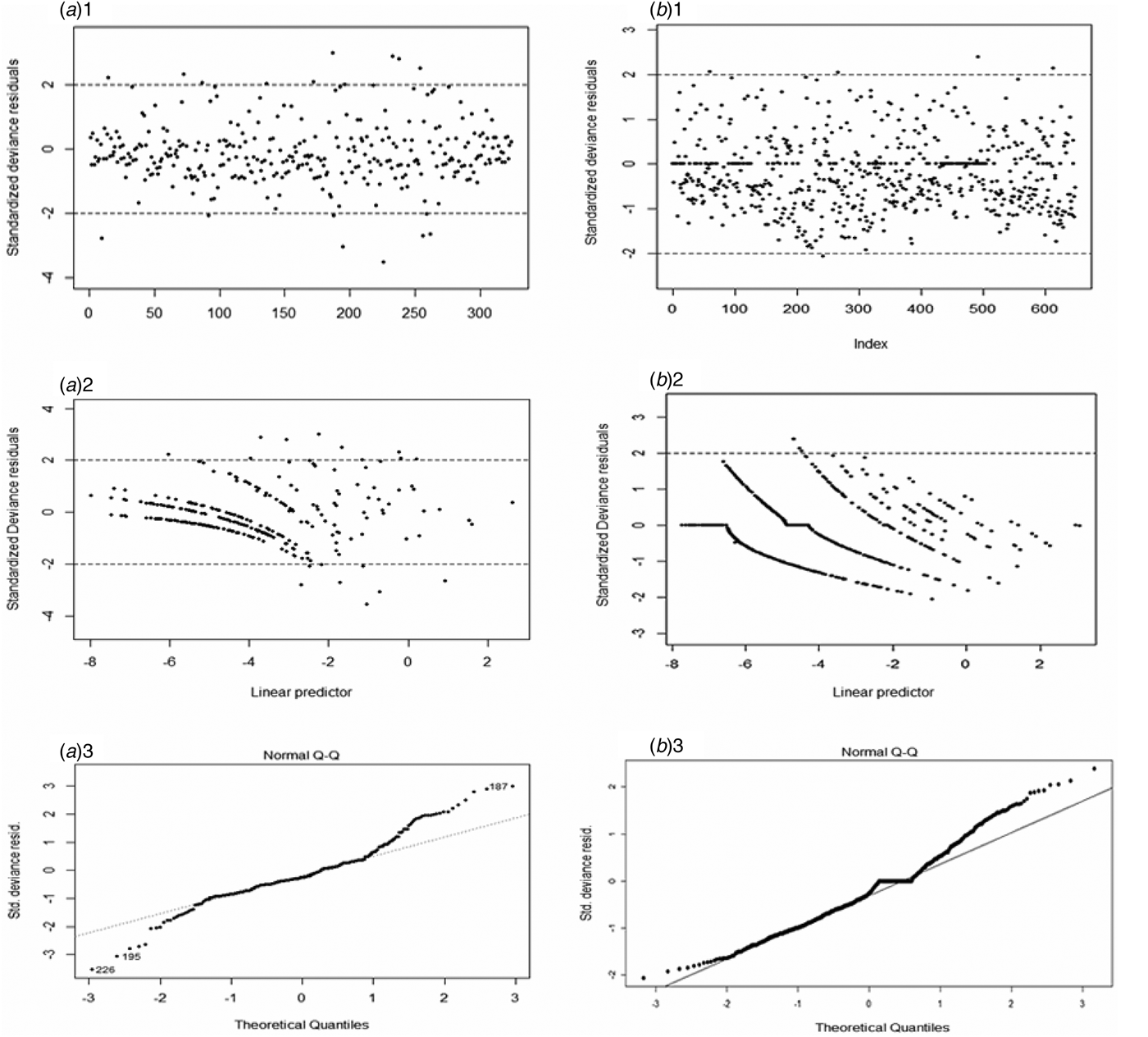
The models were fit using quasi-likelihood with the logit link function. The first model (model 1) has the variance function (μ) = μ(1 − μ) . The second model (model 2) was based on Wedderburn (Reference Wedderburn1974), in which the variance function is equal to the square of the variance of the binomial distribution, Var(μ) = [μ(1 − μ)]2. The logit link function is the linear predictor model.
The quasi-likelihood models are depicted in Fig. 3. Graphs of the standardized deviance residuals, linear predictor, index and normal QQ plot for model 1 are depicted in the first column, and those representing model 2 are depicted in the second column. Model 2 fit the data better with a more normal distribution of residuals (Fig. 3).
Graphical diagnoses for the quasi-likelihood models: Standardized deviance residuals/linear predictor, index, and Normal QQ plots; index (i), where i is the sequential order in which the values y i were measured (proportion or percentage leaf area severity affected on plot for genotypes). (A i ) Model 1, link function logit and variance function V(μ) = μ(1 − μ); (B i ) Model 2, logit link function and variance function V(μ) = [μ(1 − μ)]2.

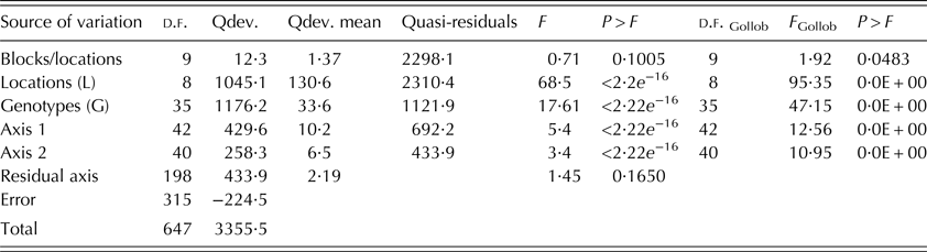
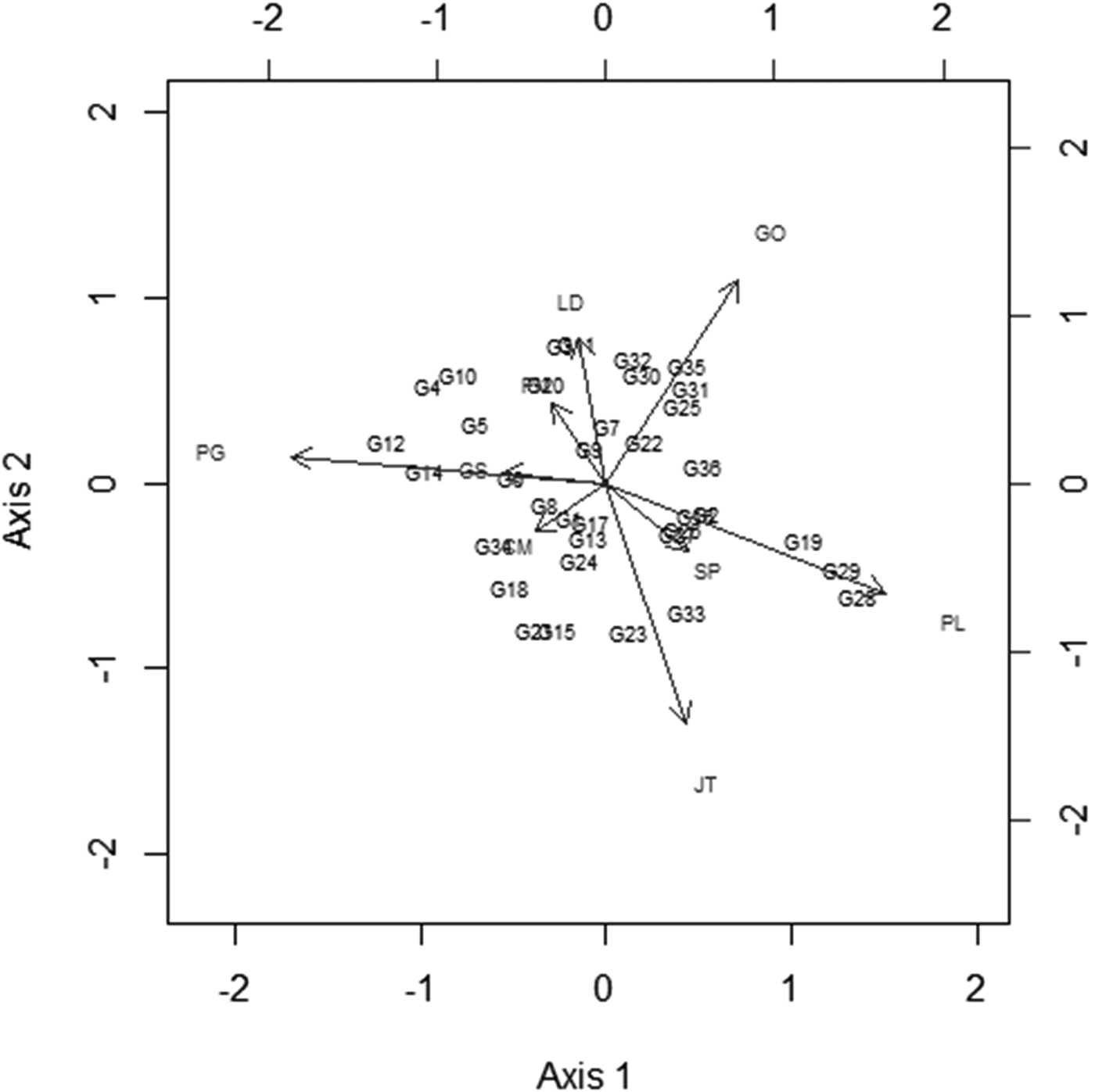
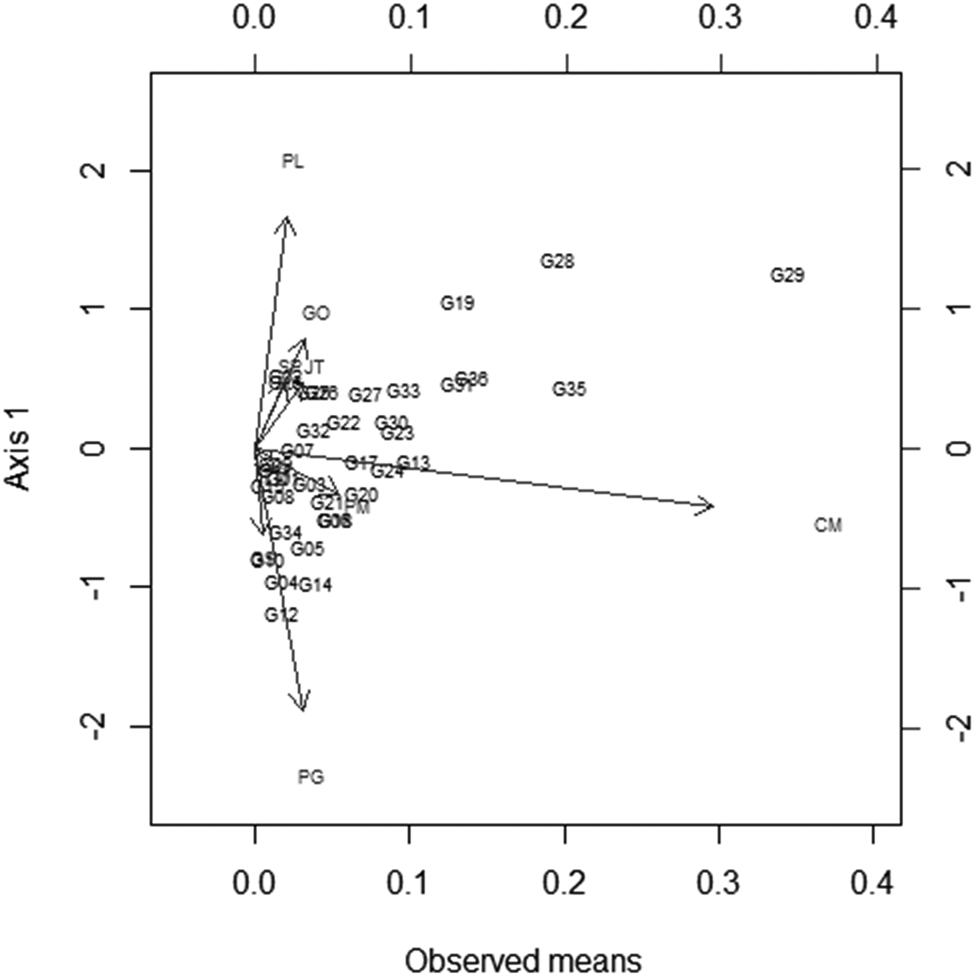
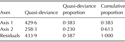
The ANODEV with the logit link function and variance function Var(μ) = [μ(1 − μ)]2 was significant for genotype and environment and also for the two first axes of the G × E interaction (Table 4). The relative contribution of genotype and environment to the interaction is shown in Fig. 4, and the genotypes with desirable low mean disease severity are shown in Fig. 5. Figure 4 describes the variability associated with the first two axes and Fig. 5 shows the relationship between the average severity of grey leaf spot and the first term of the interaction.
Analysis of deviance (ANODEV) for proportion of grey leaf spot severity, using model 2 with logit link function and variance function Var(μ) = [μ(1−μ)]2]

d.f., degrees of freedom; Qdev., quasi-deviance.
The G × E interaction for grey leaf spot severity using the GAMMI model 2 with the link function logit and variance V(μ) = [μ(1 − μ)]2. The quasi-deviance proportion of the axis 1 accounts for 38·30% of the G × E interaction and that of axis 2 accounts for 23·0% of the G × E interaction. Locations: Campo Mourão (CM), Goiânia (GO), Goianésia (GS), Jataí (JT), Londrina (LD), Ponta Grossa (PG), Planaltina (PL), Patos de Minas (PM) and São Sebastião do Paraíso (SP).

GAMMI graphic that shows the relationship between the average severity of grey leaf spot and the first term of the G × E interaction. Locations: Campo Mourão (CM), Goiânia (GO), Goianésia (GS), Jataí (JT), Londrina (LD), Ponta Grossa (PG), Planaltina (PL), Patos de Minas (PM) and São Sebastião do Paraíso (SP).

The first two components of the GAMMI graphic that contain the average severity of grey leaf spot and the first term of the G × E interaction identified Campo Mourão, Goianésia, Londrina and São Sebastião do Paraíso as locations in which the average disease severity of genotypes is less variable. The scores from these environments are close to the vertex, which indicates minimal variation between genotypes within each environment. However, the disease severity responses of these locations were distinct. For example, genotypes in Campo Mourão had low variability and high severity of grey leaf spot (36·8%).
The contributions of Goianésia, Londrina and São Sebastião do Paraíso to the G × E interaction were relatively low, as indicated by average disease severities of 0·6, 1·4 and 2·3%, respectively, in these regions (Fig. 4 and Table 3). The genotypes G9, G1 and G17 had average disease severities of 1·4, 1·9 and 7·0%, respectively, which were close to the vertex. Therefore, these genotypes can be considered stable because of their low variability for disease severity.
Although genotype G17 is stable, it had greater grey leaf spot severity than did G9 and G1 (Fig. 5 and Table 3); thus, only G9 and G1 can be recommended for use in maize breeding programmes. The genotypes shown in Fig. 4 that appear in the upper or lower quadrants on the left showed the lowest severity of grey leaf spot. The decreasing rank order of disease severity for genotypes in the upper quadrant was G12 (6ª) > G14 (17ª) > G4 (7ª) > G10 (1ª) > G5 (13ª) > G20 (23ª) > G3 (14ª) > G11 (3ª) > G6 (20ª) > G7 (12ª) > and G9 (4ª). The decreasing rank order of disease severity for genotypes in the lower quadrant was G34 (9ª) > G18 (21ª) > G21 (19ª) > G8 (5ª) > G15 (2ª) > G24 (26ª) > G13 (30ª) > G1 (8ª) > and G17 (24ª). The genotypes G32 (15ª) > G31 (31ª) > G35 (35ª) > G30 (27ª) > G25 (16ª) > and G36 (33ª) in the upper right quadrant were sequentially closest to the vertex of the 1° and 2° axes and had the highest grey leaf spot severity. The genotypes G28 (34ª) > G29 (36ª) > G19 (32ª) > G23 (28ª) > G33 (29ª) > G22 (22ª) > G2 (11ª) > G27 (25ª) > G26 (18ª) > and G16 (10ª) in the lower right quadrant had the highest grey leaf spot severity and are shown in decreasing order of disease severity.
Model 2 allowed detection of the variance associated with the G × E interaction (Fig. 4) and axis 1 and axis 2 accounted for approximately 38·3 and 23·0% of variance associated with this interaction, respectively.
The genotypes G9 and G1 were nearest to the vertex, which indicated that they were resistant to grey leaf spot and that this resistance was relatively insensitive to environmental effects due to minimal G × E interactions. However, the remaining genotypes were sensitive to environmental effects in terms of their responses to grey leaf spot and exhibited large G × E interactions.
Genotypes with specific adaptations to particular environments are generally chosen based on a positive relationship between that genotype's position and the respective environment in the same vectorial direction, such as for crop yield, for which a vector with a small angle (coincident straight line) indicates a positive correlation between genotype and environment. However, genotypes with specific adaptation for disease resistance can be identified by the inverse orientation of the vectors for genotype and environment. Thus, the best genotypes to select for adaptation to environmental conditions should be those with the lowest average grey leaf spot severity.
Genotypes with specific adaptations were those with a reverse vectorial orientation relative to the environment, according to the proposed model. Figures 4 and 5 show that genotypes G20 (0·1%) and G10 (0·0%) showed a specific adaptability to São Sebastião do Paraíso. Similarly, genotype G35 (35·0%), which had the same vectorial direction as the environment and high average disease severity, could not be recommended for Goiania, while G24 (0·0%) and G8 (0·0%) were adapted to Goiania.
The genotypes with higher specific adaptability for Ponta Grossa are G16 and G19, with average disease severities of 1%. Genotypes G3 and G11 had lower average disease severities (0·0%) and greater adaptability for Jataí. The most desirable genotypes for the Planaltina region were G12 and G4, due to their specific adaptability and disease severities of 0%. Because of their high disease severity, genotypes G29 (40·0%) and G28 (30·0%) should not be recommended for use in breeding cultivars to grow in Planaltina. G33 (0·5%) and G26 (1%) are the most appropriate genotypes to recommend for use in Patos de Mina. No genotype was particularly well adapted to the conditions of Campo Mourão. On the other hand, two genotypes could be highly recommended for use in Goianésia, G6 (0·5%) and G26 (0·5%); the latter was highly adapted to that environment.
DISCUSSION
Because the current statistical approach is not routinely applied for the analysis of disease severity data in maize under field conditions, the data distribution had to first be characterized, then the model that best fitted the data had to be determined. The suitability of the present data for the proposed model can be seen in Fig. 3. Note the random distribution of residuals around zero, which suggests a lack of correlation between the errors; the influence of error was minor, as can be seen in the Normal QQ plot (Fig. 3); points far out of alignment were not observed. Thus, the Wedderburn model with a logistic function was appropriate to describe the data set.
The ANODEV was significant for genotype and environment as well as significant for the two first axes of the interaction (Table 4). In this decomposition, the singular value represents the level of association between these factors. Because the variable response was within the interval [0, 1] the logistic link function was used. Thus, the quasi-likelihood models were evaluated with the logit link and the variance functions Var(μ) = μ(1 − μ) and Var(μ) = [μ(1 − μ)]2. Therefore, the Wedderburn model, model 2, more reliably described the data (Fig. 3).
Among the adjusted models, model 2 showed fewer discrepant values, did not violate the initial assumptions, and presented significant coefficients, so it was the most suitable model to describe the responses in these data. The cumulative proportion of quasi-deviance of the two first axes relative to the total quasi-deviance was high (61·3%) (Table 5). However, at least 75% of the total variance could be attributed to the first two PC axes (Ferreira Reference Ferreira2008). This indicates that these components could replace the n original variables without excessive loss of information. These axes measured methodological efficiency, but they could also be used to quantify the G × E interaction.
Quasi-deviance proportion in relation to the proposed axes for the mean values of grey leaf spot severity

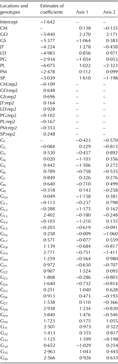
Although the basic assumptions necessary to estimate the stability and adaptability of genotypes in various environments are usually violated, the GAMMI methodology is a step forward in detecting interaction effects. Previously, the required computational methods hindered application of the GAMMI method, but specific routines are now available in R (these commands are shown Appendix A) to fit these multiplicative interaction models using van Eeuwijk's algorithm (1995). The SVD of the residual matrix used to obtain the coefficients for the main effects is shown in Table 6 together with the environment and genotype scores.
GAMMI coefficients for main effects and the scores from environments and genotypes

CM, Campo Mourão; GO, Goiânia; GS, Goianésia; JT, Jataí; LD, Londrina; PG, Ponta Grossa; PL, Planaltina; PM, Patos de Minas; SP, São Sebastião do Paraíso; Rep2, Repetition 2.
Duarte & Vencovsky (Reference Duarte and Vencovsky1999) stated that favourable combinations of genotypes and environments have coordinates with the same sign and are graphically distant from the vertex. The positive or negative interactions depicted by the biplot, principally those of high magnitude, can be useful in plant breeding programmes. For disease severity, combinations with opposite signs were of interest because they indicated genotypes suited to particular environments. Graphical representation as a biplot also permits the quick identification of more productive environments with scores of approximately zero that contribute less to the G × E interaction. Such environments could also be favourable locations for the preliminary steps of a plant breeding programme (Pacheco et al. Reference Pacheco, Duarte, Assunção, Junior and Chaves2003). Therefore, genotypes and environments with low scores for the interaction axes contribute less to model variance and are considered stable. These genotypes could be recommended for growing on large crop acreage due to their high mean crop yields and disease resistance.
In the analyses of the stability and adaptability of genotypes using multiplicative models, the interaction effects can be evaluated using graphical representations that approximate the SVD residual matrix of the model with another low rank matrix. The biplot facilitates identification and understanding of the components of the G × E interaction. Rencher (Reference Rencher2002) defined the biplot as a two-dimensional representation of the data matrix that defines the SVD produced by the SVD method. Here, the data matrix is the R (gxe), which identifies an element for every g vector of observations (g lines in the R (gxe) matrix, or genotypes) simultaneously with an element for every e variable (e columns in the R (gxe) matrix, or locations). Therefore, with this technique, one can readily identify productive genotypes with wide adaptability for mega-environments, limit genotypes with specific adaptability to determined agronomic zones, and identify the environments that should be tested (Kempton Reference Kempton1984; Gauch & Zobel Reference Gauch, Zobel, Kang and Gauch1996; Ferreira et al. Reference Ferreira, Demétrio, Manly, Machado and Vencovsky2006).
The graphic interpretation in Fig. 5 depicts the variation caused by the main additive effects of genotype and environment and the multiplicative effect of the G × E interaction (Gauch & Zobel Reference Gauch, Zobel, Kang and Gauch1996; Smith et al. Reference Smith, Cullis and Thompson2005). The abscissa represents the main effects (i.e., the overall averages of the variables for the genotypes evaluated) and the ordinate is the first interaction axis (axis 1). In this case, the lower the absolute value of axis 1, the lower its contribution to the G × E interaction; therefore, the more stable the genotype. The ideal genotype is one with high productivity and an axis 1 value near zero. An undesirable genotype has low stability associated with low productivity (Kempton Reference Kempton1984; Gauch & Zobel Reference Gauch, Zobel, Kang and Gauch1996; Ferreira et al. Reference Ferreira, Demétrio, Manly, Machado and Vencovsky2006).
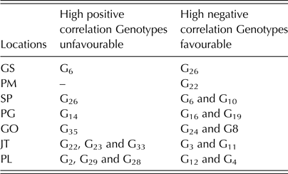
In the biplot analysis shown in Fig. 4, the cosine of the angle between a vector and an axis indicates the contribution of that variable to the axis dimension. Also, the cosine of the angle between the vectors for two environments approximates their correlation. Therefore, when vectors are perpendicular, the cosine of the angles between them equals zero and the variables are independent. But if the vectors for two variables are at very close angles or at a 180° angle, they are highly positively or negatively correlated (Gower Reference Gower and Krzanowski1995; Kroonenberg Reference Kroonenberg1997). The angles between the vectors for sites and genotypes, and the positions of the vectors, permitted us to identify genotypes positively or negatively correlated with particular environments (Table 7).
Genotypes positively or negatively associated with specific environments

GS, Goianésia; PM, Patos de Minas; SP, São Sebastião do Paraíso; PG, Ponta Grossa; GO, Goiânia; JT, Jataí; LD, Londrina; PL, Planaltina.
The negative correlation between cultivar and location has helped to identify genotypes with specific adaptations. Genotypes with a highly negative correlation within an environment had the lowest disease severities (Fig. 4 and Fig. 5), and should therefore be recommended for use in those locations.
CONCLUSIONS
The GAMMI method efficiently described the data regarding stability and adaptability of genotypes to grey leaf spot incidence in various locations in Brazil using available theories and the computational resources outlined in the present paper. A pattern of differential responses to grey leaf spot in different environments was found, and the GAMMI method could explain 61·3% of the variance due to the G × E interaction with only two PC. The two-dimensional analysis detected the presence of a strong interaction between genotype and environment.
The GAMMI model could efficiently identify and quantify the G × E interactions, even though the data were not normally distributed and variances were heterocedastic. The present analyses indicated that the genotypes G9 and G1 could be recommended because of their high stability and low severity of grey leaf spot. Campo Mourão, Goianésia, Londrina, and São Sebastião do Paraíso were locations in which average disease severity was more stable, indicating that these locations made a minor contribution to the G × E interaction. The scores from these environments had values close to the vertex in the figures, which indicated less variability among genotypes for disease severity. However, the responses to disease in these locations were distinct. For example, Campo Mourão exhibited low variability and high severity of grey leaf spot (36·8%). Genotypes with specific adaptability and low severity of grey leaf spot for specific locations were G26 for Goianésia, G24 and G8 for Goiânia, G3 and G11 for Jataí, G19 and G16 for Ponta Grossa, G12 and G4 for Planaltina, G26 and G33 for Patos de Minas, and G10 and G20 for São Sebastião do Paraíso. These results will be useful to guide recommendations of cultivars with stable resistance to grey leaf spot and high yield in particular environments.
Appendix A
The multiplicative term of this model was estimated in R software with the generalized nonlinear models gnm function using the Mult (factor 1, factor 2, inst = …) command, which specifies the multiplicative interactions that are linear or nonlinear predictors. The subscripts 1 and 2 represent the multiplicative factors of the interaction and inst is an integer that specifies the number of interactions (Turner & Firth Reference Turner and Firth2009). The function residSVD (model, fac1, and fac2, d = …) performed the SVD of the residual matrix. This residSVD function uses the first d components of the SVD to approximate a residual vector from the model by adding d multiplicative terms (Turner & Firth Reference Turner and Firth2009). Finally, the model is re-adjusted by the update command (object, formula … evaluate = TRUE), which assumes the coefficients from the previous model as starting values for the new model.