1.1 Contemporary methods for data reduction

Today’s high-fidelity computational fluid dynamics (CFD) and high-end experimental data acquisition systems tend to produce vast amounts of data that are getting harder to interpret and overview. Methods to analyse such data are numerous and are always developing to stay in line with acquisition and computation systems. The most challenging data stem from turbulent flows that feature a huge range of temporal and spatial scales. A key challenge in turbulent flow data mining is the distinction of deterministic coherent motion from purely stochastic motion. Numerous methods exist that exploit the periodicity or energetic dominance of these coherent structures. These methods range from classic Fourier decomposition to dynamic mode decomposition (DMD) and proper orthogonal decomposition (POD). The most prominent among them are briefly introduced in the following.

POD has been widely used since its introduction by Lumley (Reference Lumley1970) and Sirovich (Reference Sirovich1987). It was applied in nearly every fluid dynamic field. Beyond fluid dynamics, this method is also known as singular value decomposition, principal component analysis or Karhunen–Loève expansion (Berkooz, Holmes & Lumley Reference Berkooz, Holmes and Lumley1993). The basic idea behind this method is to construct an optimal basis that represents most of the data variance with as few basis functions as possible. In the context of POD the variance is turbulent kinetic energy. Therefore, the POD searches for the most energetic modes whereby coherent structures with high energy content are likely to be represented by POD basis functions (Holmes et al. Reference Holmes, Lumley, Berkooz and Rowley2012).

Another classical approach is the linear stochastic estimation introduced by Adrian & Moin (Reference Adrian and Moin1988), where the readings of different sensors are related via a linear mapping. This is closely related to the extended POD (Boree Reference Boree2003), also described in a unified framework (observable inferred decomposition) by Schlegel et al. (Reference Schlegel, Noack, Jordan, Dillmann, Gröschel, Schröder, Wei, Freund, Lehmann and Tadmor2012). In recent extensions of linear stochastic estimation, the use of time delays between the different sensors and also the use of one sensor at multiple time instances are pursued to separate periodic coherent structures from turbulent fluctuations (Durgesh & Naughton Reference Durgesh and Naughton2010; Lasagna, Orazi & Iuso Reference Lasagna, Orazi and Iuso2013). This approach was also used to improve the determination of harmonic POD modes from few pressure sensors (Hosseini, Martinuzzi & Noack Reference Hosseini, Martinuzzi and Noack2015). These utilizations of data from various time instances are also related to the temporal constraint used for the POD extension proposed in this article.

Targeting the temporal periodicity of the coherent structures, spectral methods such as discrete Fourier transform (DFT) and the recently introduced DMD (Rowley et al. Reference Rowley, Mezic, Bagheri, Schlatter and Henningson2009; Schmid Reference Schmid2010) come into play. These methods commonly span the mode space according to fixed frequencies, which enables the identification of coherent structures within small spectral bandwidths. In contrast to DFT, DMD also distinguishes modes with respect to their linear amplification. The recently introduced extended DMD (Williams, Kevrekidis & Rowley Reference Williams, Kevrekidis and Rowley2015) tries to overcome the limitations encountered by the (linear) DMD approach when trying to decompose data from nonlinear systems. The idea is to use nonlinear functions that create observables of the data, which are exactly described by a linear system. This approach translocates the problem towards the identification of these nonlinear functions, which can be solved using the ‘kernel trick’ that is common in machine learning. This paper presents an alternative approach, which extends POD to account for temporal dynamics in addition to energetic optimality.

1.2 Why yet another method?

After this short and incomplete review of data processing methods, one may ask if there is need for another method. The answer is probably no, so we take the most used method (POD) and bring it up to date for present research issues. The approach pursued here includes a simple yet effective extension to the classical POD, which leads to a more general method comprising POD and also DFT. This approach unifies existing methods, but also offers possibilities beyond these. From the authors’ experience, the currently available methods often fail when applied to challenging flow data. These stem from flows with weak coherent structures where the recorded data have low signal-to-noise ratios, from flows with intermittent dynamics, or from flows featuring multi-modal interactions leading to frequency modulations, to name a few. In such cases, much effort is required to optimize the data processing until satisfactory results are obtained. The usual escape route is to focus on a certain spatial region or to apply suitable filters to pick out a certain wavelength or frequency range. This involves trial and error or requires prior knowledge of the investigated flow. There is also the danger of cutting off a substantial portion of the data, leading to false interpretations. These procedures can be collected under the heading ‘identifying symmetries’ as done by Holmes et al. (Reference Holmes, Lumley, Berkooz and Rowley2012). The drawback of this approach is that the investigated flow must feature some symmetries and they must be known a priori. A recent application shows the huge variety of spatial and temporal filtering together with POD to separate different phenomena into different modes (Bourgeois, Noack & Martinuzzi Reference Bourgeois, Noack and Martinuzzi2013), exemplifying the complexity of this approach.

The usage of spectral methods for highly turbulent flows is even more challenging than POD. The variable frequency of single coherent structures and intermittent occurrence of different structures with the same frequency hinders a proper decomposition. In terms of the DFT, averaging of spectra from multiple measurements or sensors is essential to obtain reliable results. Analogously, for DMD, averaging over several events is an option to reject noise (Tu et al. Reference Tu, Rowley, Luchtenburg, Brunton and Kutz2014). Nonetheless, the results obtained with DFT and DMD suffer from limiting the temporal dynamics to single frequencies. Turbulent flows hardly ever feature discrete frequencies and it is not always valuable to restrict a single mode (flow phenomenon) to a single frequency. Coherent structures that feature significant phase jitter or frequency modulation are represented by many modes at similar frequencies. In contrast, the POD puts no temporal constraint on the modes. This can result in modes that represent flow phenomena occurring at largely different temporal scales. Thus, it is often hard to interpret these modes and draw meaningful conclusions from the temporal dynamics.

From our point of view, there is a big gap between the energetically optimal decomposition of POD and the spectrally clean decomposition of DFT or DMD. This gap will be bridged with the spectral proper orthogonal decomposition (SPOD) introduced in this article. This new method not only places itself somewhere in between these two extrema, but it allows for a continuous shifting from one to the other. The main idea is to apply a filter operation to the POD correlation matrix, which will force the POD towards clear temporal dynamics. Depending on the filter strength we continuously sweep from classic POD to DFT.

The remainder of this article is organized as follows: the proposed method is described in detail in § 2. The reader is guided from snapshot POD via an in-depth interpretation of the correlation matrix towards the general description of the SPOD. In addition, a method is explained to identify coupled mode pairs describing a single coherent structure, which becomes handy when working with SPOD. In § 3, the new method is demonstrated on three different experimental data sets. The results are compared against POD and DFT to point out the benefits of SPOD. In § 4 the capabilities of SPOD are summarized, based on the findings from the application to experimental data.

2.1 Classical snapshot POD

To introduce the method and the nomenclature, the snapshot POD approach is described first. We start off with a decomposition of a data set into spatial modes and temporal coefficients:

Note that only the fluctuating part $u^{\prime }(\boldsymbol{x},t)$ is decomposed. It is split into a sum of spatial modes ${\it\Phi}_{i}$ and mode coefficients $a_{i}$ . A set of $M$ spatial points recorded simultaneously over $N$ time steps is considered. To calculate the POD, the correlation matrix of this data set is needed. For data obtained from particle image velocimetry (PIV) or CFD, the number of spatial points is usually larger than the number of snapshots. The correlation matrix is then calculated between individual snapshots (temporal correlation). The alternative approach (spatial correlation) that applies to $M\ll N$ is detailed in appendix A. The correlation between two snapshots is calculated from an appropriate inner product $\langle \,,\rangle$ , usually defined as the $L^{2}$ inner product

where $V$ specifies the spatial region or volume over which the correlation is integrated. The elements of the correlation matrix $\unicode[STIX]{x1D64D}$ are given by

Matrix $\unicode[STIX]{x1D64D}$ is of size $N\times N$ .

The temporal coefficients $\boldsymbol{a}_{i}=[a_{i}(t_{1}),\ldots ,a_{i}(t_{N})]^{\text{T}}$ and mode energies ${\it\lambda}_{i}$ are obtained from the eigenvectors and eigenvalues of the correlation matrix:

The subscript $i$ refers to single eigenvalues, which are sorted in descending order. Since the $\boldsymbol{a}_{i}$ are the eigenvectors of the real symmetric positive-definite matrix $\unicode[STIX]{x1D64D}$ , they are orthogonal. Moreover, they are scaled with the energy of the single modes such that

where $(\,,\,)$ denotes the scalar product. The spatial modes are obtained from the projection of the snapshots onto the temporal coefficients:

These modes are orthonormal by construction, i.e.

The formulation so far is perfectly in line with classical snapshot POD, which can also be computed by a singular value decomposition. However, since the SPOD requires a manipulation of the correlation matrix we retain the classical form.

2.2 Properties of the correlation matrix

The SPOD described in this article is essentially a filter applied to the correlation matrix $\unicode[STIX]{x1D64D}$ . To offer a better understanding of this approach, the structure of the correlation matrix $\unicode[STIX]{x1D64D}$ is inspected first.

Figure 1.

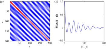
(a) Pseudo-colour plot of the correlation matrix elements $\unicode[STIX]{x1D619}_{i,j}$ and (b) the corresponding correlation coefficient $\widehat{R}$ . The displayed data are selected from PIV measurements of a forced turbulent jet.

Figure 1(a) shows the structure of the correlation matrix for the data set of a forced turbulent jet. The data were acquired with PIV inside a 2-D plane aligned with the jet axis. The considered flow shows strong vortex shedding at the forcing frequency (the acquisition frequency is 25 times the forcing frequency). The presence of these periodic patterns in the flow, and their convection within the observed flow field, leads to a diagonal, wave-like structure of the matrix. This is closely related to the periodicity of the autocorrelation coefficient. In fact, if the individual elements of the correlation matrix $\unicode[STIX]{x1D64D}$ are summed up along the diagonals, we obtain the spatially averaged autocorrelation coefficient

where the upper bound $T$ is the length of the measured sequence. This is depicted in figure 1(b), showing the same periodicity as the correlation matrix. The autocorrelation coefficient itself represents the spectral content of different time scales and wavelengths and it is directly related to the power spectral density of the underlying data. However, it contains no information on the phase of individual frequencies, due to the reference of the signal to itself. This is why the elements along the diagonals of $\unicode[STIX]{x1D64D}$ look so similar, as they represent only relative changes with respect to the time step on the main diagonal. Thus, increased similarity along the diagonals of $\unicode[STIX]{x1D64D}$ is equivalent to an increased similarity of the dynamics of the underlying signal. This property will be discussed in more depth in § 2.4. The obvious consequence from these findings is: if we want to obtain smooth dynamics from the POD, we have to enforce the diagonal similarity of the correlation matrix. This is where we step into spectral POD.

2.3 General description of the SPOD

The yet so simple but radical approach is a filter operating on the correlation matrix $\unicode[STIX]{x1D64D}$ . To augment the diagonal similarity of $\unicode[STIX]{x1D64D}$ a simple low-pass filter is applied along the diagonals. This results in a filtered correlation matrix $\unicode[STIX]{x1D64E}$ with the elements given as

The filter above is just a symmetric finite impulse response filter with a filter coefficients vector $\boldsymbol{g}$ of length $2N_{f}+1$ . The most simple approach would be a box filter, where all coefficients have the same value $g_{k}=1/(2N_{f}+1)$ . In the examples discussed later, we use a Gaussian filter, which features a smooth response in time and frequency domain. Moreover, we choose a standard deviation such that the filter gives the same cutoff frequency as a box filter with half the length. In fact, any kind of digital finite impulse response filter can be used here.

The further procedure of the SPOD is the same as for the classical POD. From the filtered correlation matrix $\unicode[STIX]{x1D64E}$ the temporal coefficients $\boldsymbol{b}_{i}$ and mode energies ${\it\mu}_{i}$ are obtained from the eigendecomposition

The temporal coefficients are also scaled with the mode energy and they are still orthogonal:

The spatial modes are finally obtained from the projection of the snapshots onto the temporal coefficients,

where these modes are no longer orthogonal. This property of the spatial modes is detailed in appendix B. The total energy of the data set is still represented by the decomposition ( $\sum {\it\lambda}_{i}=\sum {\it\mu}_{i}$ ), but the energy per mode is less for the first modes. Hence, increasingly plain temporal dynamics is obtained at the expense of spatial orthogonality and a dispersed SPOD spectrum. Nevertheless, the decomposition (as in (2.1))

is still exact if all $N$ SPOD modes are used for the recomposition.

Figure 2.

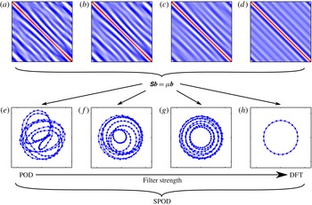
Schematic describing the main properties of the SPOD for increasing filter strength (from left to right): (a,e) $N_{f}=0$ ; (b,f) $N_{f}=25$ ; (c,g) $N_{f}=100$ ; (d,h) $N_{f}=200$ . (a–d) Pseudo-colour plots of the filtered correlation matrix ( $\unicode[STIX]{x1D64E}$ ). (e–h) The phase portraits of the corresponding first two modes ( $\boldsymbol{b}_{1}$ and $\boldsymbol{b}_{2}$ ) that describe the dominant oscillations. The axes of the plots shown here are the same as for the plots in figures 1 and 16, respectively. The graphs are based on the data already presented in § 2.2 and the SPOD is calculated from 200 snapshots.

If the filter size is extended over the entire time series, the filtered correlation matrix converges to a symmetric Toeplitz matrix. This matrix has the form

with the diagonals given by the average correlation coefficient (2.8). This special matrix is also known as the covariance matrix and its eigenvalues trace out the power spectral density of the underlying time series (Wise Reference Wise1955). This equality is a part of Szegö’s theorem and it is valid for the limiting case where the number of samples approaches infinity. To discuss this feature for finite series, the treatment of the start and end of the time series must be clarified. At the boundaries of $\unicode[STIX]{x1D64D}$ , the filter operation is not properly defined, since the symmetric filter lacks elements before and after the finite series. Either these elements can be replaced by zeros or the time series is assumed to be periodic. For the zero padded boundary, $\unicode[STIX]{x1D619}_{i,j}=0$ in (2.9) for any $i$ or $j$ that is outside of the domain $[1,N]$ . In the case of periodic boundary conditions, indexing outside of the valid domain is mapped back into the domain by addition or subtraction of $N$ (e.g. $\unicode[STIX]{x1D619}_{i,j}=\unicode[STIX]{x1D619}_{i-N,j}$ if $i>N$ ). For periodic conditions and a box filter of the same size as the number of snapshots, a symmetric circulant matrix is obtained, where the eigenvalues and eigenvectors are given by the Fourier transform of the first row (Gray Reference Gray2005). Hence, DFT and SPOD produce the same decomposition for this limiting case. For the Gaussian filter this limit is only exactly reached with a infinitely large filter size, but practically, the decomposition remains nearly constant for values $N_{f}>N$ . In the following example of application, the DFT is calculated with $N_{f}=N$ and a box filter.

The general SPOD approach and its placement with respect to the existing methods are graphically summarized in figure 2. The images in the first row show the filtered correlation matrix at different filter widths $N_{f}$ . The images below depict the phase portraits of the leading two modes (compare figure 16). It is apparent that the increased diagonal similarity of the correlation matrix, which goes in hand with the increased filter width, successively limits the temporal variations of the mode amplitude and frequency until a stable limit cycle is reached. In summary, the SPOD allows for continuous fading from the energetically optimal POD to a purely spectral DFT. What happens in between these two limits is very promising, as will be shown later in this article.

2.4 Spectral properties of the SPOD filter operation

Now provided with the continuous transition between POD and DFT, we may determine how the SPOD filter affects the resulting mode dynamics. In other words, we would like to know how the filter frequency response transfers into mode space. This enables the choice of an adequate filter size $N_{f}$ , which is the crucial property of the introduced filter operation.

We consider the forced turbulent jet data already consulted in the previous section. In this flow the periodic shedding is strong and regular and it is represented by the same SPOD mode regardless of the filter setting. Furthermore, the flow is turbulent, showing sufficient jitter and broadband noise in the mode dynamics to demonstrate the effect of the SPOD filter. Figure 3 shows the spectrum of the most dominant SPOD mode coefficient $b_{1}$ computed for different filter sizes $N_{f}$ . According to these graphs, the SPOD operation applies a band-pass filter to the modal dynamics with the band centred around the dominant frequency. The width of the band and the spectral attenuation are directly related to the filter width.

Figure 3.

Magnitude of the frequency spectrum for the first SPOD mode for different filter widths $N_{f}$ . The analysed flow is the forced turbulent jet presented in figures 1 and 2.

The spectral response of the filter coefficients $\boldsymbol{g}$ that define the spectral constraint (2.9) of the SPOD are drawn in figure 4. As described in the previous section, these coefficients are chosen to represent a Gaussian filter with a typical low-pass characteristic, where the cutoff frequency is related to the filter width by $f_{c}\propto 1/N_{f}$ .

Figure 4.

Magnitude of the SPOD filter frequency response for different filter widths $N_{f}$ .

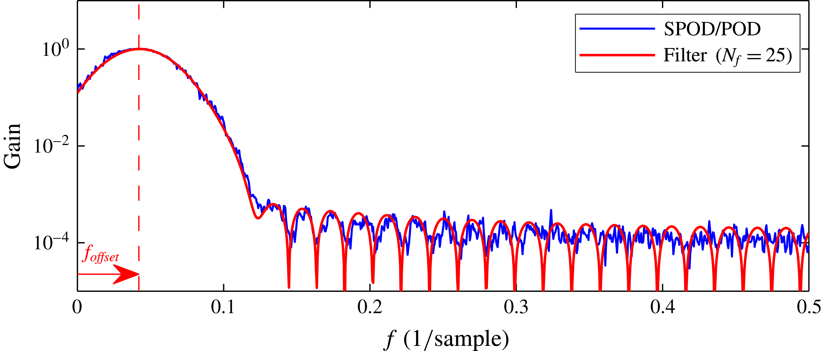
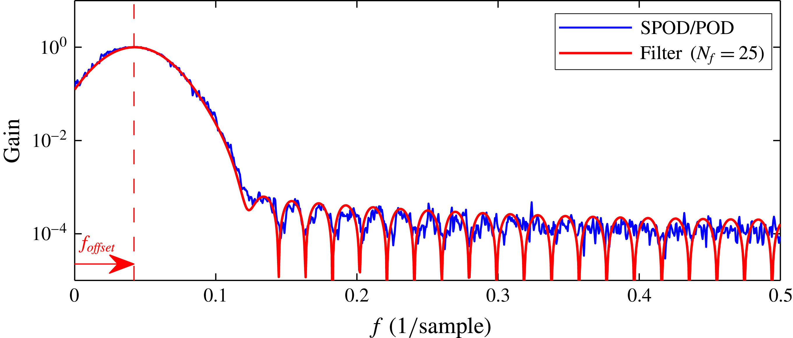
To evaluate the frequency response of the entire SPOD method, we compute the spectral attenuation of the SPOD with respect to POD and compare this to the frequency response of the filter coefficients. The spectral attenuation is calculated from the ratio of spectral magnitudes of the first SPOD ( $N_{f}=25$ ) and POD ( $N_{f}=0$ ) coefficients $b_{1}$ . The results are shown in figure 5, where the graph of the filter frequency response must be shifted to compensate for the difference between low- and band-pass filtering. Accordingly, both curves show nearly the same attenuation as well as the same characteristic stop-band ripples. In this adapted representation the spectral attenuation of the SPOD can be directly estimated from the filter coefficients. However, the SPOD shows a band-pass characteristic while the filter coefficients describe a low-pass filter. The frequency around which the band is centred is selected intrinsically by the SPOD.

Figure 5.

The spectral attenuation of the SPOD obtained from the ratio of the spectral magnitudes $|\mathscr{F}(b_{N_{f}=0})|/|\mathscr{F}(b_{N_{f}=25})|$ and the response of the filter coefficients $|\mathscr{F}(g)|$ from (2.9). For the filter response the frequency axis is offset to match the modes’ centre frequency.

The band-pass behaviour of the SPOD is a direct consequence of the smoothing of the diagonal elements of the correlation matrix. As elaborated in appendix C for linear system dynamics, variations of the diagonal elements relate directly to variations of the frequency and amplification of the modes. Hence, the SPOD filter operation constrains the temporal variation of the mode frequency and amplification rate, but sets no limitations on the temporal mean frequency and amplitude. Thus, the SPOD filter averages out frequency variations, which reduces the spectral bandwidth of the modes. With the selected low-pass filter coefficients, the smoothing intensity can be adjusted, which controls the bandwidth of the filter. However, the selection of a centre frequency for this band-pass filter is data driven, which means the filter ‘snaps’ to a dominant (coherent) fluctuation contained in the data.

Based on these conclusions, an adequate filter size $N_{f}$ may be selected prior to the SPOD. Ideally, it should be a time span for which the coherent structures of interest exhibit constant dynamics. In practice, we found that suitable selections for this time span are the characteristic time scales of the flow. These are either one period of a dominant oscillation or the time that a structure needs to be convected a typical length scale of the flow.

Based on the coefficient spectra shown in figure 3, it may seem that SPOD is just a method that is comparable to a subsequent band-pass filtering of POD modes, but the situation is substantially different. A posterior filtering of POD modes cuts out parts of the temporal dynamics that are ignored in further investigations. In the case of the SPOD, the filter is applied prior to the decomposition. Hence, the filter shifts the dynamic content removed from one mode to the other modes. Therefore, the entire dynamic content is still represented in the decomposition, but it is redistributed among the modes (2.13). Moreover, the SPOD may ‘find’ modes that were hidden in noise or mixed with other modes, which is not possible with a subsequent filter.

2.5 Identification of coupled modes

One crucial point in POD and SPOD is the identification of linked modes. Assuming the presence of periodic coherent structures, their dynamics is described by a pair of modes, analogues to the sine and cosine in the Fourier space or the real and imaginary parts of DMD modes. They constitute the real and imaginary parts of an analytical signal,

where $A$ is the amplitude and ${\it\phi}$ the phase of the signal ( $\text{i}=\sqrt{-1}$ ). The coupling of such a mode pair is not given by the SPOD and it has to be identified a posteriori. Coupled modes typically show a similar amount of energy and pair in the POD spectrum (Oberleithner et al. Reference Oberleithner, Sieber, Nayeri, Paschereit, Petz, Hege, Noack and Wygnanski2011; Oberleithner, Rukes & Soria Reference Oberleithner, Rukes and Soria2014). For more complex dynamics with multiple energetic modes, the pairs are not easily identified and visual inspection of Lissajous figures and spatial modes is required. This manual procedure is cumbersome and by no means objective.

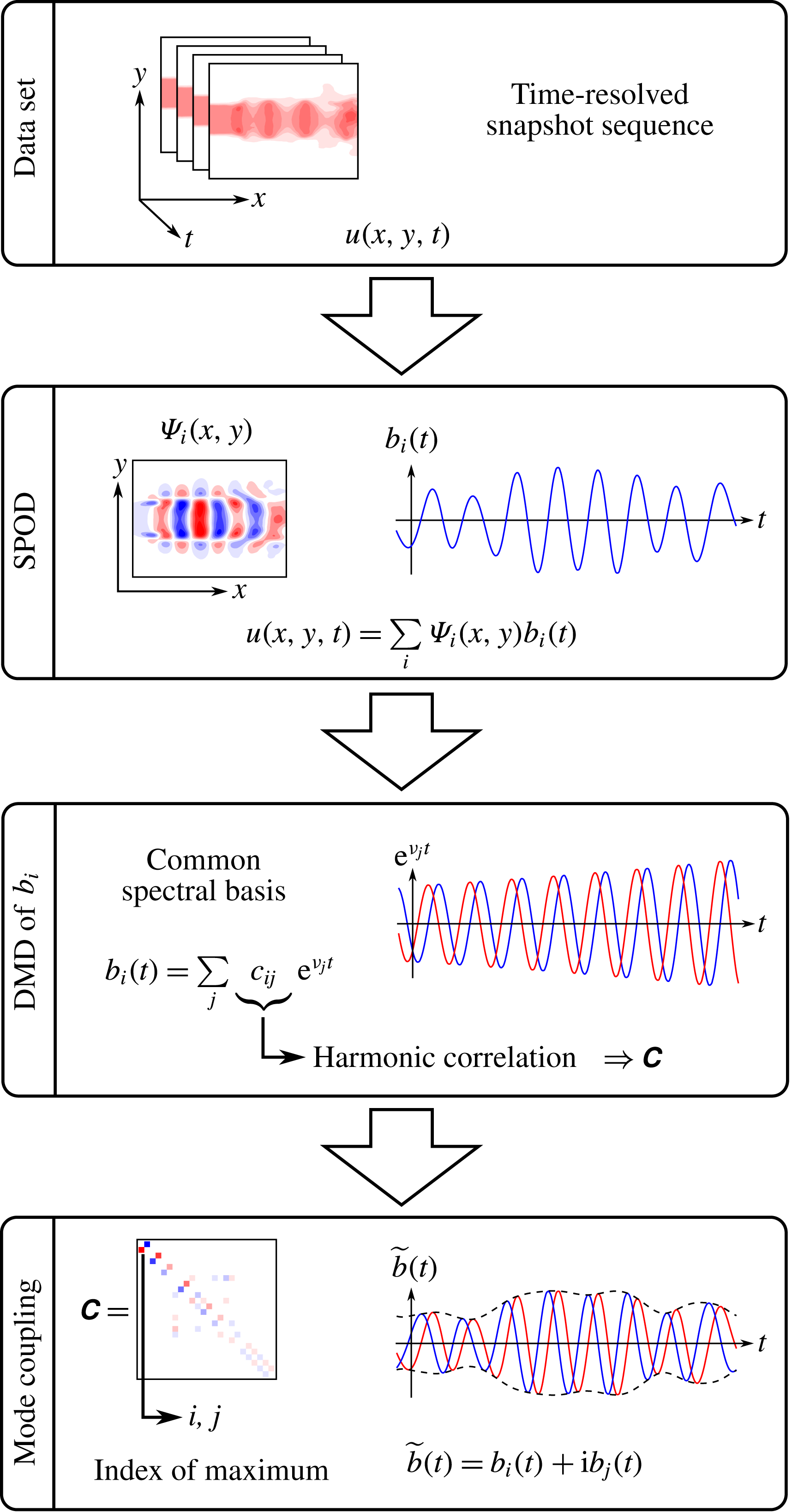
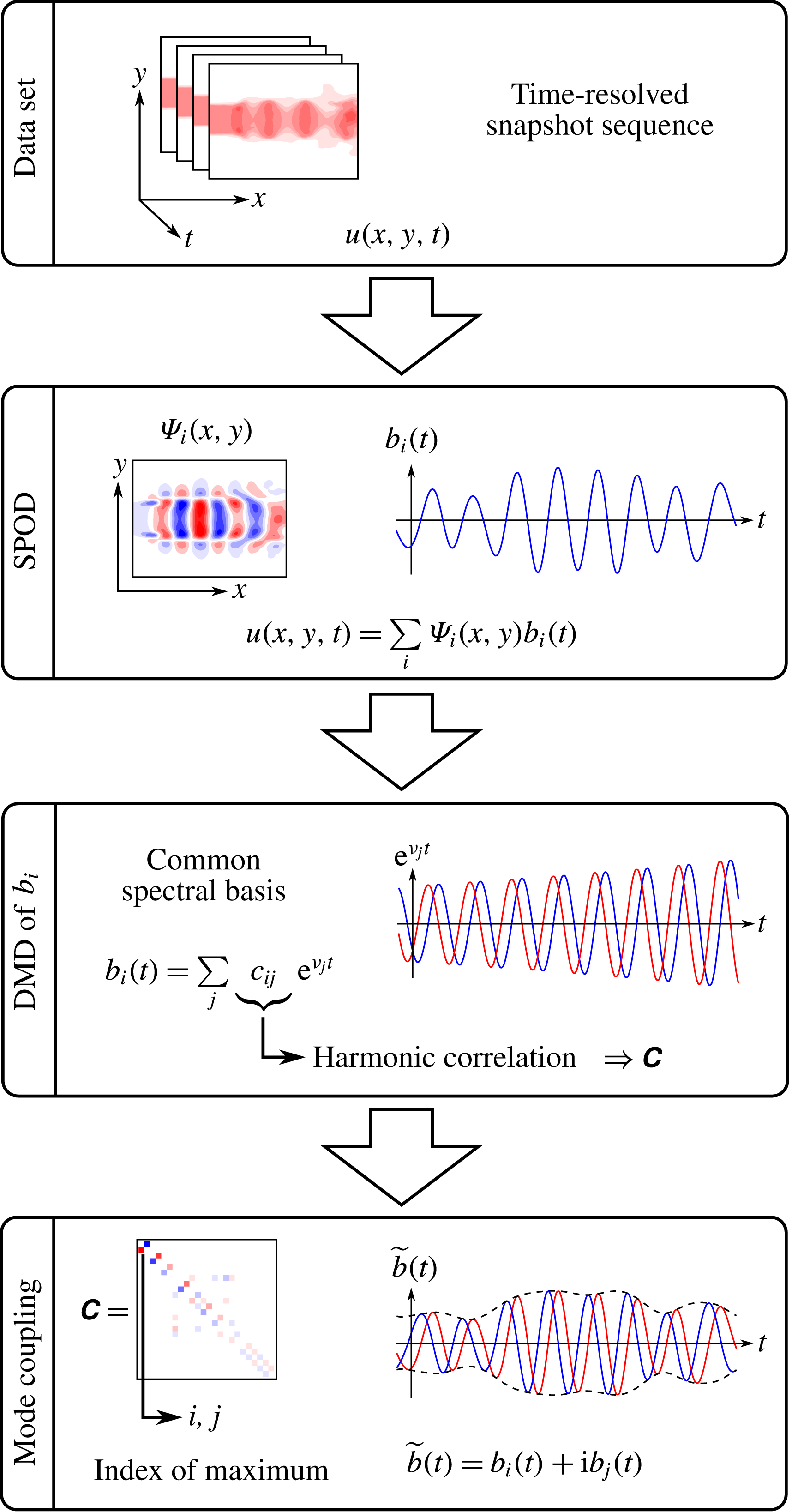
To provide an alternative, we propose an unbiased approach that gives a quantitative measure of the dynamic coupling of individual modes. The idea is to evaluate the mode coefficients cross-spectra at a ${\rm\pi}/2$ phase lag, in order to measure the spectral proximity. Mode pairs that describe a single structure must have the same spectral content, but are shifted by a quarter period. In the following, this spectral measure is also called harmonic correlation. Fourier decomposition and DMD were both considered to evaluate this harmonic correlation, but the DMD turned out to be more reliable for this task. The general procedure is schematically outlined in figure 6. From the depicted operations, the DMD and the mode coupling are discussed in this section.

Figure 6.

Schematic illustrating the main steps towards the identification of coupled modes (red and blue lines indicate real and imaginary parts of an analytic signal). The data displayed here were derived from measurements of a forced turbulent jet (see also figure 1).

For the DMD of the SPOD coefficients, their temporal evolution is assumed to be governed by a linear operator $\unicode[STIX]{x1D64F}$ ,

To approximate this operator, the SPOD coefficients are arranged in two matrices $\unicode[STIX]{x1D653}=[\boldsymbol{b}(0)~\boldsymbol{b}({\rm\Delta}t)\cdots \boldsymbol{b}((N-2){\rm\Delta}t)]$ and $\unicode[STIX]{x1D654}=[\boldsymbol{b}({\rm\Delta}t)~\boldsymbol{b}(2{\rm\Delta}t)\cdots \boldsymbol{b}((N-1){\rm\Delta}t)]$ (following the notation of Tu et al. (Reference Tu, Rowley, Luchtenburg, Brunton and Kutz2014)). Hereafter, the operator is given by

where $\unicode[STIX]{x1D653}^{-1}$ is the Moore–Penrose pseudo-inverse of $\unicode[STIX]{x1D653}$ . Alternatively, this can be solved as a least squares problem, minimizing $\Vert \unicode[STIX]{x1D64F}\unicode[STIX]{x1D653}-\unicode[STIX]{x1D654}\Vert$ . To reject measurement noise in the identification procedure, only the ‘physical part’ of the SPOD modes is considered for the calculation of the operator $\unicode[STIX]{x1D64F}$ . That means only the modes with acceptable signal-to-noise ratio should be considered. Therefore, the number of retained modes is calculated from the energy resolved by the SPOD, truncated after $N_{c}$ modes, with

In the examples shown later the modes are truncated around $\mathscr{E}(N_{c})=0.95$ . This value depends on the signal-to-noise ratio of the considered measurement, which can be estimated from the POD spectrum (Raiola, Discetti & Ianiro Reference Raiola, Discetti and Ianiro2015). Note that the number of retained modes increases for wider SPOD filters and correspondingly flatter SPOD spectra ( ${\it\mu}_{j}$ ).

The DMD modes are obtained by the eigendecomposition of matrix $\unicode[STIX]{x1D64F}$ as

The eigenvalues ${\it\nu}_{i}$ comprise the frequencies ${\it\omega}_{i}$ and amplification rates ${\it\sigma}_{i}$ of the operator $\unicode[STIX]{x1D64F}$ , which are related to the logarithm of the eigenvalue via $\ln ({\it\nu}_{i})/{\rm\Delta}t={\it\sigma}_{i}+\text{i}{\it\omega}_{i}$ . The eigenvectors $\boldsymbol{c}_{i}$ hold the relative spectral content of the single SPOD coefficients with respect to these frequencies. More precisely, the element $c_{i,j}$ of vector $\boldsymbol{c}_{i}$ is the spectral content of the single mode coefficient $b_{j}$ with respect to ${\it\nu}_{i}$ . The actual modal representation is given by

It must be noted that this decomposition is only exact if $N_{c}=N$ , whereas in the current approach $N_{c}<N$ . Nevertheless, the decomposition gives a common spectral basis, which allows the ranking of spectral similarity of the temporal coefficients $\boldsymbol{b}(t)$ . The developed proximity measure is given by

where $^{\ast }$ indicates the complex conjugate and the coefficients are normalized so that $(\boldsymbol{c}_{i},\boldsymbol{c}_{i})=1$ . The sign function ( $\text{sgn}$ ) in this expression accounts for the conjugate pairs that appear in the DMD spectrum (mirrored at the real axis).

For two modes to be coupled, they must have a similar spectral content, which is shifted a quarter period forward or backward. This implies a positive or negative imaginary part of the harmonic correlation (2.21), respectively, and coupled modes appear as peaks in the matrix $\unicode[STIX]{x1D63E}$ . Hence, the row and column indices of the maximum of $\unicode[STIX]{x1D63E}$ identify the first coupled SPOD modes. The corresponding row and column in $\unicode[STIX]{x1D63E}$ are then set to zero and the next lower maximum is identified. This procedure is repeated until all modes are paired. It has to be noted that this approach also creates weakly correlated and possibly unphysical mode pairs.

Together with the identification of coupled modes, the procedure gives an average frequency of the coherent structure represented by the mode pair. Therefore, the eigenvalues ${\it\nu}_{k}$ of the matrix $\unicode[STIX]{x1D64F}$ are sorted in descending order with respect to their content for the identified mode pair $\widetilde{c}_{k}=c_{k,i}^{2}+c_{k,j}^{2}$ . The frequency is given as the weighted sum of the eigenvalues,

The weighting accounts for the relative energy content of a mode pair with respect to the single frequencies. In fact, only the most relevant eigenvalue ( $n=1$ ) can be chosen to determine the frequency, but for practical application it is recommended to use more than one eigenvalue as noise may corrupt them. For the examples discussed in the next chapter, we used an average over three eigenvalues ( $n=3$ ) to obtain accurate results.

The coupled SPOD modes are considered as one complex mode (see (2.15) and figure 6) similar to the Fourier mode. The relative energy content of the identified modes is computed as

where $i$ and $j$ again refer to the indices of the coupled SPOD modes.

3.1 Swirling jet undergoing vortex breakdown

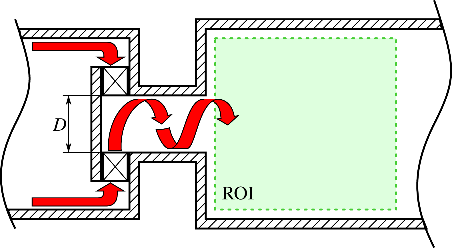
First, we consider the flow field of a swirl-stabilized combustor. Swirling jets are widely used in the gas turbine industry due to their capability of obstacle-free flame anchoring and enhanced mixing. The experimental set-up to study these flows is sketched in figure 7. Swirl is generated by injecting fluid tangentially into a mixing tube that terminates in the combustion chamber. The cylindrically shaped chamber is made of quartz glass to allow optical access for PIV. Flow measurements are conducted in the meridional section as indicated in the schematic. The case investigated here is non-reacting at a Reynolds number of 58 000 based on the nozzle diameter $D$ and the bulk velocity at the nozzle exit. Additional details about the experimental set-up can be found in Reichel, Terhaar & Paschereit (Reference Reichel, Terhaar and Paschereit2015).

Figure 7.

Experimental set-up of the swirl-stabilized combustor. Air enters from the left, passes a swirl generator and exits into the combustion chamber. Flow field measurements with PIV are conducted in the meridional plane indicated by the dashed square (ROI).

Figure 8.

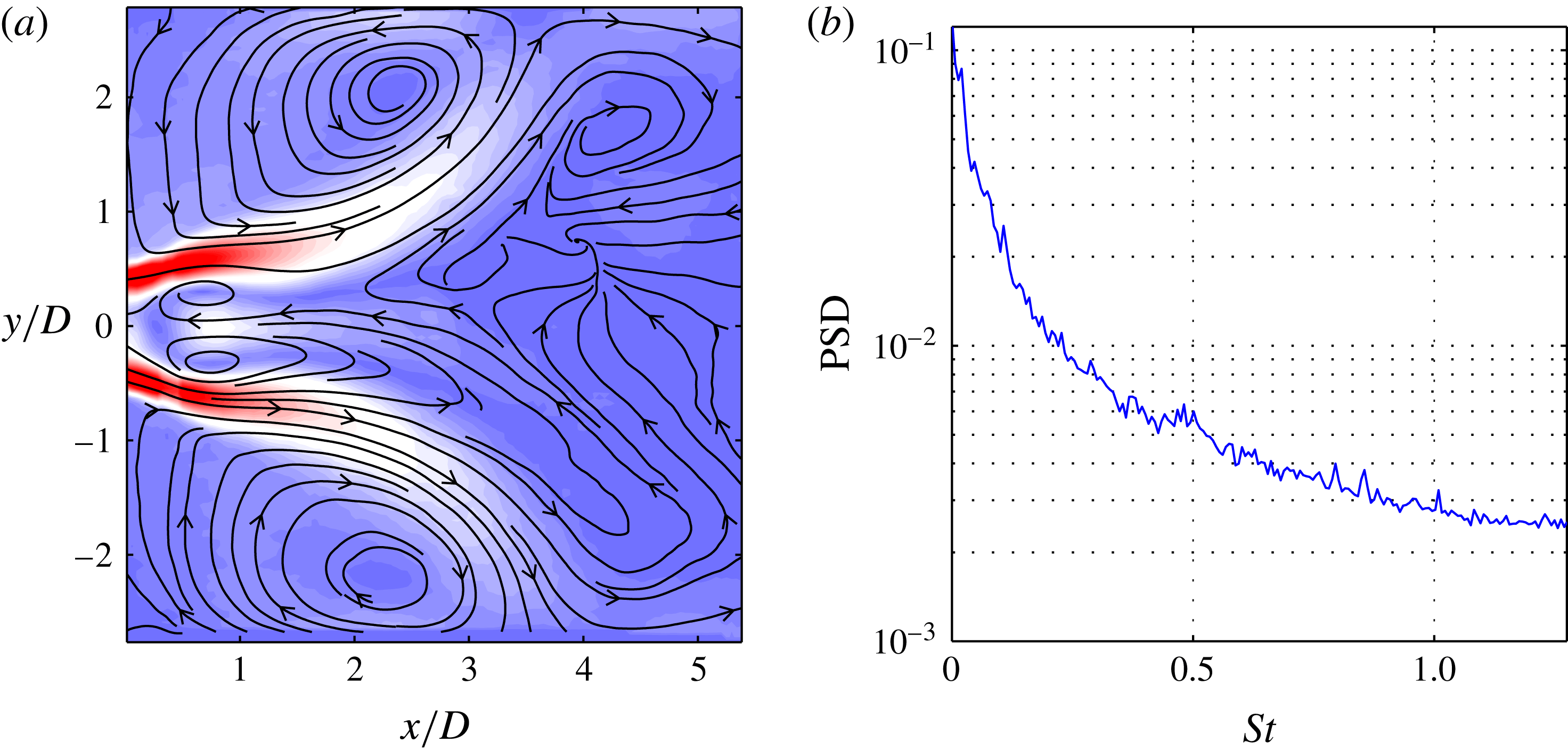
Swirl-stabilized combustor flow: time-averaged flow field depicted by (a) contours of velocity magnitude and streamlines, and (b) spatially averaged power spectral density.

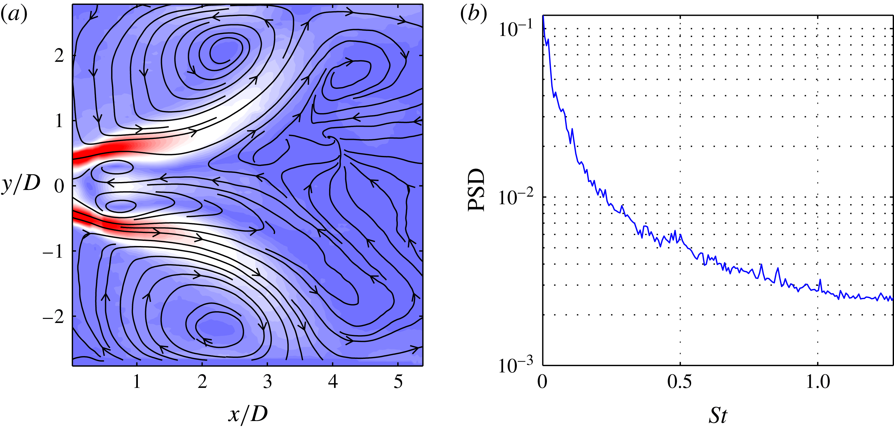
The mean flow field and the spatially averaged power spectral density (PSD) are depicted in figure 8, with the Strouhal number based on the same length and velocity scale as the Reynolds number ( $St=f\,D/u_{bulk}$ ). The flow exhibits a strong recirculation zone in the centre, surrounded by an annular, strongly diverging jet. The cross-sectional jump at the combustion entrance creates an additional external recirculation zone between the jet and the confining walls. The spectral content of the flow is spread over all time scales and it decreases with increasing Strouhal number. The spectrum gives no indication of any dominant coherent structure even though these flows typically feature helical global modes (Oberleithner et al. Reference Oberleithner, Sieber, Nayeri, Paschereit, Petz, Hege, Noack and Wygnanski2011).

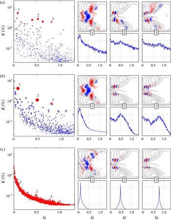
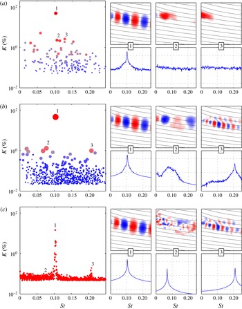
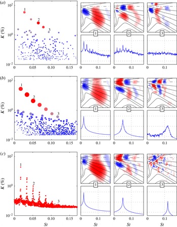
Figure 9(a–c) illustrate the results from the SPOD for the filter lengths $N_{f}=0$ , 10 and 2000, respectively. Note that the limiting cases $N_{f}=0$ and $N_{f}=2000$ produce results equivalent to those obtained with classical POD and DFT respectively, while the case in between represents the SPOD. Hence, this particular presentation concisely demonstrates the difference between POD, SPOD and DFT.

Figure 9.

Swirling jet: results from SPOD for different filter lengths (a)  $N_{f}=0$ (POD), (b) $N_{f}=10$ (SPOD) and (c) $N_{f}=2000$ (DFT). For each filter length the SPOD spectrum is displayed as a scatter plot (left), where a single dot indicates one mode pair (size and colour $C_{i,j}$ in (2.21)). For three selected pairs the spatial modes (upper row) and PSD of the temporal coefficient (lower row) are depicted. They are indicated by numbers in the SPOD spectrum, as well as between the small mode plots.

Each of the three cases in figure 9 shows the so-called SPOD spectrum, where every mode pair is represented by a single dot. The size and colour of the dots indicate the harmonic correlation of a mode pair $C_{i,j}$ , according to (2.21). The frequency of a mode pair is determined according to (2.22) and the energy from the two eigenvalues relative to the total energy from (2.23). On the right side of every case in figure 9, three spatial modes ${\it\Psi}_{i}(\boldsymbol{x})$ and the corresponding temporal coefficients $b_{i}(t)$ are plotted above each other. The spatial modes are visualized by the cross-wise velocity component (in the $y$ -direction) together with streamlines of the time-averaged flow. They are numbered likewise in the SPOD spectrum and in the small mode plots. The plots are given without axis labels to allow a compact representation of the data; the section is the same as for the mean flow shown in figure 8(b). The time coefficients are represented by their power spectral density, where the time series is split into five (50 % overlapping) sections, which are Fourier transformed and averaged. The horizontal dotted lines in the PSD plots indicate a spacing of three orders of magnitude ( $10^{3}$ ) and the $y$ -axis is scaled logarithmically. The spectral averaging was also applied to the power spectra shown in figure 8(b) and in the subsequent PSD plots.

The POD (figure 9 a) yields a broad spectrum of modes, where modes at lower Strouhal numbers have more energy. There are several modes with high harmonic correlation (diameter and colour of the points) and high energy content $K$ . The spatial shape of the low-frequency mode (label 1) shows clear spatial symmetry and a limited spectral bandwidth ( $St\approx 0.1$ ). This mode is frequently observed in swirl-stabilized combustors and it is associated with a global hydrodynamic instability (Terhaar, Oberleithner & Paschereit Reference Terhaar, Oberleithner and Paschereit2015). From the four additional outstanding modes between $St=0.3$ and $St=0.8$ , we choose two for further investigation. Their spatial structures cannot be precisely assigned to a symmetric or anti-symmetric mode and they indicate mixtures of several spatial wavelengths. Accordingly, the mode spectra are broad and show only a slight hump at the frequencies indicated by the SPOD spectrum. The other modes around $St=0.5$ , which are not shown here, show similar spatial and spectral content.

Overall, the POD indicates the presence of a single mode at low frequency, together with other coherent structures that are not properly resolved. The most energetic mode (not inspected here) corresponds to a low-frequency, large-wavelength fluctuation, as indicated by the SPOD. Such slow changes of the mean flow are usually called shift modes (Luchtenburg et al. Reference Luchtenburg, Günther, Noack, King and Tadmor2009; Hosseini et al. Reference Hosseini, Martinuzzi and Noack2015). In this particular case the shift mode stems from weak movements of the vortex breakdown bubble.

Consider now the SPOD in figure 9(b), with a filter length $N_{f}=10$ ; from the SPOD spectra we identify three peaks at $St=0.09$ , 0.5 and 0.8. The first mode is the same as the one already identified by the POD, but its spectral content at higher frequencies is reduced. It describes a single-helical structure in the wake of the recirculation zone. The second identified mode exhibits a broad spectral peak at $St=0.5$ . Its spatial structure and Strouhal number match the global mode identified by Oberleithner et al. (Reference Oberleithner, Sieber, Nayeri, Paschereit, Petz, Hege, Noack and Wygnanski2011). It is a single-helical mode linked to the precessing motion of the recirculation zone. The spatial structure of mode three suggests a double-helical shape. It is not a harmonic of the second mode, as their frequencies are not related.

When the filter size is extended to its maximum, the DFT (figure 9 c) and SPOD spectrums converge to the spatially averaged PSD (figure 8 b). The temporal coefficients converge to sines and cosines and all mode pairs show full harmonic correlation (uniform dot size in the SPOD spectrum). Since selection based on harmonic correlation is impossible, we resort to the frequencies already known from the SPOD at $N_{f}=10$ . The spatial structures resemble the ones from figure 9(b), but they are corrupted by noise. Moreover, the spatial symmetries are no longer as clear as for the $N_{f}=10$ case. Note that the corresponding spectral peaks are broadened due to the averaging procedure, which is applied here only for consistency.

From this first example, we can point out some striking features of the SPOD. The SPOD is able to separate coherent fluctuation from stochastic turbulent fluctuations even though they both have the same energy content (see the SPOD spectrum in figure 9 c). The classical POD yields partially mixed structures that cannot be assigned to distinct flow phenomena, whereas the SPOD properly separates these structures and identifies them from harmonic correlations. The DFT instead shows the same structures at the identified frequencies, but they are corrupted with noise and the method itself would give no clue about the frequencies of interest.

The structures identified with the SPOD may also be found with the POD if the decomposition is applied to a subsection of the measured domain. Moreover, the exploitation of spatial symmetries prior to the POD decomposition usually provides good results for this type of flows (Terhaar Reference Terhaar2015). Nevertheless, these alternative approaches would require prior knowledge of the shape or spatial extent of the structures, whereas the SPOD requires none of these.

All modes identified by the SPOD show clear spatial symmetries and distinct spectral peaks. The frequency and shape of the first mode coincide well with previous experimental observations in swirl-stabilized combustors (Terhaar et al. Reference Terhaar, Oberleithner and Paschereit2015). The second mode is very similar to the one observed in unconfined swirling jets (Oberleithner et al. Reference Oberleithner, Sieber, Nayeri, Paschereit, Petz, Hege, Noack and Wygnanski2011). However, the presence of these different modes in a single flow configuration raises the question regarding their physical relevance. To deal with this issue, we conducted a linear stability analysis of the underlying mean flow, following the procedure outlined by Oberleithner et al. (Reference Oberleithner, Stöhr, Seong, Arndt and Steinberg2015). This analysis similarly delivered three unstable modes whose frequencies and azimuthal and axial wavenumbers match the SPOD modes surprisingly well. To limit the scope of this paper the analysis is not further detailed here. One important parameter of the SPOD is the filter size $N_{f}$ , which is twice the period of the second mode. The experiences gained throughout the first application show that a filter size of one to two periods of the mode of interest gives the best results.

3.2 Airfoil with Gurney flap

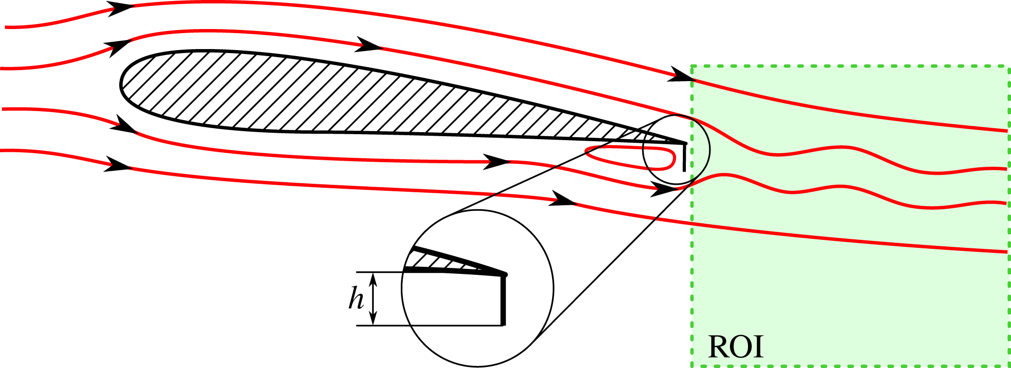
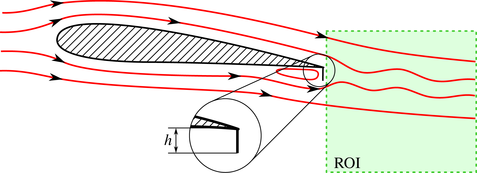
The second flow configuration considered here is the flow behind a pitched airfoil equipped with a Gurney flap. The experimental set-up is shown in figure 10. It illustrates the working principle of the Gurney flap deployed at the pressure side of the airfoil. The flap creates additional lift (and drag), which can be used to locally control varying loads on large wind turbine airfoils (Bach et al. Reference Bach, Lennie, Pechlivanoglou, Nayeri and Paschereit2014, Reference Bach, Berg, Pechlivanoglou, Nayeri and Paschereit2015a ). The flow features around the Gurney flap are characterized by a single vortex that develops upstream of the flap and periodic shedding in its wake. The vortex upstream of the flap continuously grows up to a critical size, then it is shed into the wake, and it starts growing again. Here, a FX 63-137 airfoil at $5^{\circ }$ angle of attack is investigated at a Reynolds number of 180 000 based on chord length. The reference length for the Strouhal number is the flap height, which is 3.6 % of the chord. The measured region comprises only the wake of the airfoil capturing the dominant vortex shedding. More details about the experimental set-up can be found in a previous publication on these data (Bach et al. Reference Bach, Pechlivanoglou, Nayeri and Paschereit2015b ). The Strouhal number in the following results is calculated with the flap height $h$ and the free stream velocity.

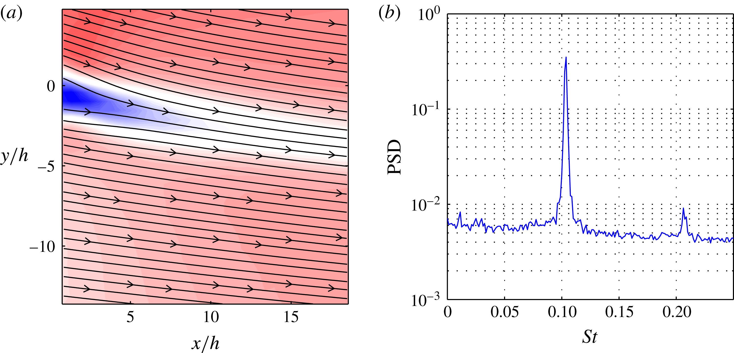
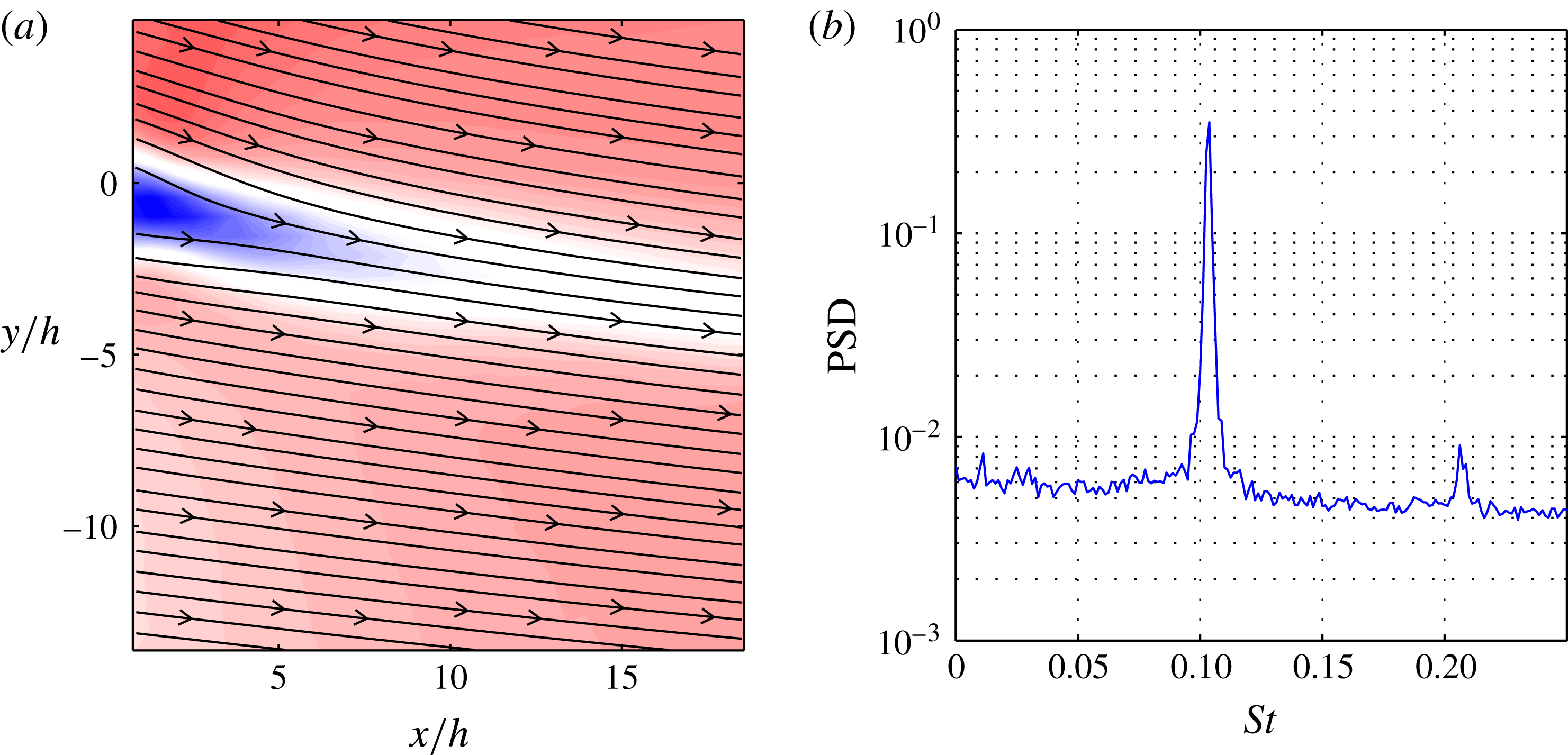
The mean flow shown in figure 11(a) reveals a velocity deficit in the wake of the Gurney flap, which generates the vortex shedding. The PSD (figure 11 b) indicates strong oscillations at $St=0.105$ with a weak higher harmonic. In a previous investigation it was found that the vortex, which is shed from upstream of the flap, causes an alteration of the periodic vortex shedding behind the flap (Troolin, Longmire & Lai Reference Troolin, Longmire and Lai2006). Hot-wire measurements in the wake of the Gurney flap supported this assumption. The combination of a strong periodic flow pattern and the intermittent short-time events provides a formidable benchmark for the SPOD.

Figure 10.

Schematic of the airfoil equipped with a Gurney flap at the trailing edge. Streamlines indicate the surrounding flow and the vortex upstream of the flap. The measured section (ROI) is a streamwise cut in the wake of the airfoil, capturing the periodic shedding behind the flap.

Figure 11.

Wake of the airfoil with Gurney flap: time-averaged flow field depicted by (a) contours of velocity magnitude and streamlines, and (b) spatially averaged power spectral density. The origin of the coordinate system is located at the trailing edge.

Figure 12.

Airfoil with Gurney flap: results from SPOD for different filter lengths (a) $N_{f}=0$ (POD), (b) $N_{f}=15$ (SPOD) and (c) $N_{f}=2000$ (DFT). For each filter length the SPOD spectrum is displayed as a scatter plot (left), where a single dot indicates one mode pair (size and colour $C_{i,j}$ in (2.21)). For three selected pairs the spatial modes (upper row) and PSD of the temporal coefficient (lower row) are depicted. They are indicated by numbers in the SPOD spectrum, as well as between the small mode plots.

The presentation of the decomposition with the different methods is organized in the same way as for the previous example. The classic POD decomposition is shown in figure 12(a). The vortex shedding is represented by the most energetic POD mode with the highest harmonic correlation. The remaining modes show weak harmonic correlations and no distinct peak in the SPOD spectrum. The modes labelled 2 and 3 exhibit a broad spectral content with a spatial extent limited to the vicinity of the flap. There are additional modes with similarly compact spatial extent located further downstream. These compact modes describe the intermittent alteration of the vortex shedding during the passage of the single vortex that was generated upstream of the Gurney flap. An inspection of their time coefficients (not shown) reveals that these modes are only active one after another during one shedding period. Depending on the phase lag between the natural oscillation and the shedding of the upstream vortex, the developing wake vortex is either strengthened or weakened. The convection of this altered vortex is described by a spatial series of modes. The modes 2 and 3 represent only the upstream part of this convection, while the additional modes located further downstream (not shown) describe the subsequent motion. This behaviour is indicated by a complex interaction of these modes and the periodic shedding modes, which is hard to identify in the POD expansion.

The SPOD yields a much clearer set of modes (figure 12 b). In addition to the shedding mode, the SPOD also uncovers three other modes, which are offset from the rest. The two modes that appear at similar frequencies capture the alteration of the vortex shedding during the passage of the single vortex. Their mode shape is similar to the shedding mode, but with larger spatial wavelengths and lower frequencies (see mode 2 in figure 12 b). The interaction of the upstream vortex with the vortex shedding increases the vortex size and thus the wavelength in the wake. Assuming a constant convection speed in the flow, this mode consequently has a lower frequency. In the case of the SPOD the alteration of the vortex shedding is captured by a single mode (pair) and is thus much easier to interpret. The third mode represents the second harmonic of the vortex shedding, with a clear spectral peak and clean spatial mode with twice the wavelength of the shedding mode. This higher harmonic is completely missed in the POD. The SPOD filter size $N_{f}$ is equivalent to three shedding periods, which is approximately equal to the travelling time through the measurement domain.

The DFT shown in figure 12(c) reproduces the spectrum shown in figure 11(b). The natural mode and its higher harmonic can be identified from the spectral peaks. The corresponding mode shapes are similar to the SPOD, although the higher harmonic is corrupted with noise, resulting in a fragmented spatial mode. The DFT at the frequency of the second SPOD mode gives no indication of the structure identified before and the vortex–vortex interaction is completely missed. This is attributed to the fact that this phenomenon is highly intermittent with varying frequencies and amplitudes, which cannot be represented by a single-frequency mode. The same dilemma applies for the DMD.

For this example, the SPOD has shown its ability to separate dynamics with similar spatial structures and frequencies but very different energies. The spectral proximity and spatial similarity of the involved dynamics impede the application of POD. The modulation of the natural vortex shedding is represented by a natural mode with several intermittent modes. The DFT, however, with its single-frequency modes does not capture the modulation of the shedding at all. The frequency constraint imposed by the SPOD is sharp enough to split the natural shedding from the modulation and soft enough to allow for frequency and amplitude variations. Hence the SPOD again gives easy access to dynamic features of the flow, which cannot be found with other common methods of similar algorithmic complexity. There may be feature tracking approaches capable of identifying the dynamics in this case, but they usually require more computational effort and might not be as versatile as the SPOD.

Figure 13.

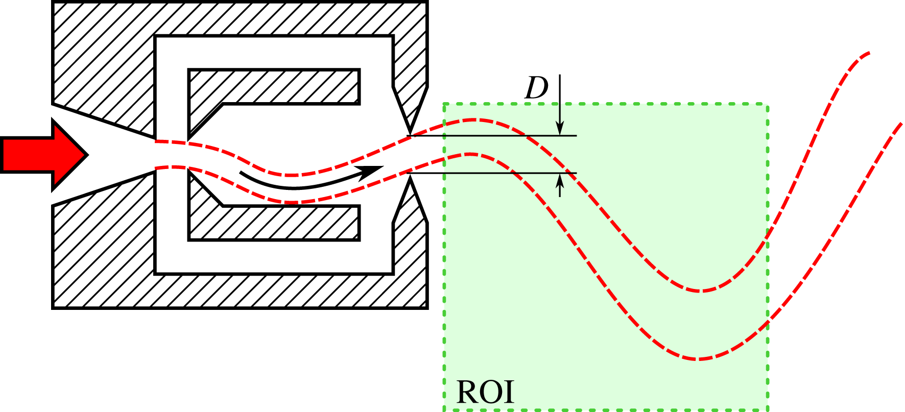
Schematic of the experimental set-up with the fluidic oscillator. Air enters from the left, passes the oscillator and exits into the unconfined ambient air. The angle of the jet leaving the oscillator sweeps periodically up and down. The measured region (ROI) captures the meridional plane of the jet’s near field. The oscillator has a square nozzle, hence the thickness of the jet normal to the plane is also D.

Figure 14.

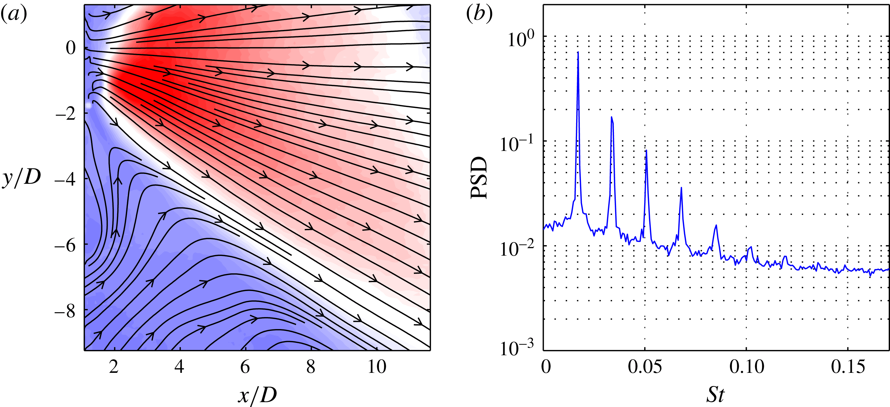
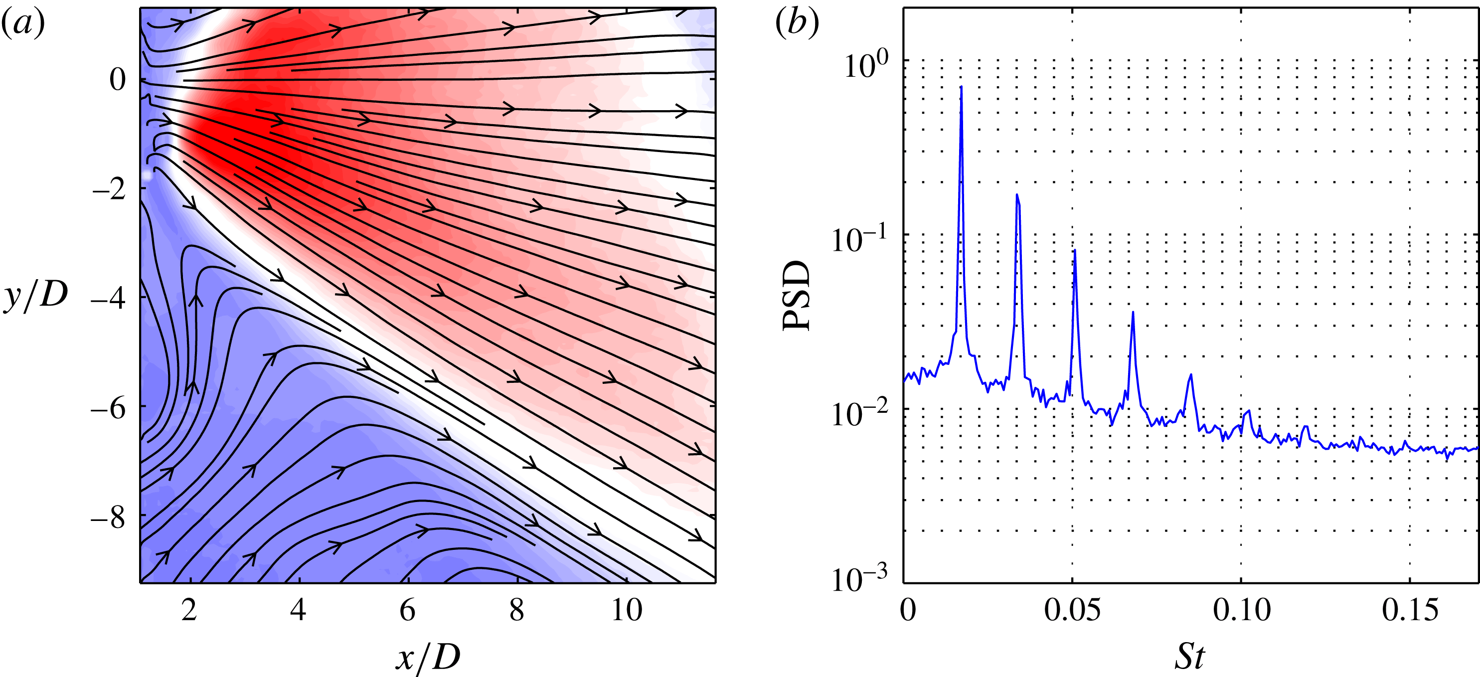
Fluidic oscillator: time-averaged flow field depicted by (a) contours of velocity magnitude and streamlines, and (b) spatially averaged power spectral density.

3.3 Fluidic oscillator

In this example, SPOD is applied to the flow field of the sweeping jet generated from a fluidic oscillator. This device is essentially a nozzle with feedback channels, which cause a self-sustained oscillation of the jet. Figure 13 shows the approximate geometry of this device and indicates the meandering shape of the sweeping jet. The shape and motion of the jet resemble a travelling wave. These devices are used for active flow control applications, where the sweeping motion of the jet allows a much wider actuator spacing, resulting in less energy consumption (Woszidlo et al. Reference Woszidlo, Stumper, Nayeri and Paschereit2014). The data presented here stem from an experimental set-up investigating the spreading and entrainment of sweeping jets (Ostermann et al. Reference Ostermann, Woszidlo, Nayeri and Paschereit2015b ; Woszidlo et al. Reference Woszidlo, Ostermann, Nayeri and Paschereit2015). The data are recorded at a Reynolds number of 37 000 based on the nozzle diameter $D$ and the mean velocity in the nozzle. These scales are also used for later calculation of the Strouhal number. The mean velocity in figure 14(a) shows that the PIV domain is moved off the jet centre towards the lower half of the jet. Data points closer than $x/D=2$ were distorted due to laser light reflections. The spectral content averaged over the PIV domain (figure 14 b) shows a narrow dominant peak and at least five higher harmonics. The narrow peaks indicate a stable operation at the fundamental frequency, while the additional peaks suggest more complex dynamics. The key challenge of this data set is to accurately reconstruct the sweeping jet dynamics from a truncated measurement domain.

Figure 15 shows the results from the SPOD for filter lengths $N_{f}=0$ , 30 and 2000. As in the foregoing examples, these filter settings span the range between both limiting cases (from the POD to the DFT). The spectrum attained with the POD (figure 15 a) reveals distinct modes at the fundamental frequency of the oscillator (labelled 1) and at higher harmonics. The mode at the third harmonic frequency (labelled 2) shows a surprisingly high harmonic correlation. The PSD of the mode coefficients reveals that each mode is not limited to a single frequency. The additional peaks in the PSD are partly attributed to the fact that only part of the jet is measured. During one oscillation period, the jet leaves and enters the measurement domain, creating sharp transitions in the time domain and thus a series of higher harmonics in the frequency domain. Due to the purely statistical POD approach, these higher harmonics appear in every mode coefficient, which contradicts the idea of a proper modal decomposition. The mode that seems to represent the fifth harmonic in the SPOD spectrum (labelled 3) shows no distinct peak at all in the PSD of the coefficient. Thus, the POD of this data set does not provide a proper separation of the fundamental and higher harmonic contributions.

Figure 15.

Fluidic oscillator: results from SPOD for different filter lengths (a) $N_{f}=0$ (POD), (b) $N_{f}=30$ (SPOD) and (c) $N_{f}=2000$ (DFT). For each filter length the SPOD spectrum is displayed as a scatter plot (left), where a single dot indicates one mode pair (size and colour $C_{i,j}$ in (2.21)). For three selected pairs the spatial modes (upper row) and PSD of the temporal coefficient (lower row) are depicted. They are indicated by numbers in the SPOD spectrum, as well as between the small mode plots. The centreline is indicated by a dash–dotted line.

If the SPOD is applied instead, the fundamental and harmonic modes line up perfectly (figure 15 b). Now, the harmonics are separated clearly up to seventh harmonics. The spectral content and spatial shape are further examined for the fundamental, third and seventh harmonics. The PSDs of the mode coefficients reveal narrow spectral bands. The corresponding mode shapes show an appropriate spatial symmetry, although the PIV domain is cropped shortly above the symmetry line. It is worth mentioning that the broad peak in the PSD of the seventh harmonic indicates considerable frequency jitter, while the mode shape remains remarkably smooth and symmetric.

The results obtained with the DFT are presented in figure 15(c). The peaks in the SPOD spectrum clearly indicate the fundamental and the first five higher harmonics. Their spatial shapes agree well with the SPOD modes, which is not surprising as these modes have narrow spectral bands. Note, however, that each peak is split into several DFT modes, which indicates slight frequency variation. This becomes crucial for the higher harmonics, where the frequency jitter is significant and the mode energy is low. For the seventh harmonic, the DFT fails to reproduce the structure seen in the SPOD (figure 15 b). The frequency variations detected by the SPOD are simply too high and the mono-frequent energy content too low. This emphasizes the superior noise rejection of the SPOD.

In this example, SPOD is superior to POD and DFT. The energy-ranked POD modes primarily suffer from the incompleteness of the data set. This is of immense importance as the relevant domain size is rarely known prior to a set of experiments or POD analysis. The frequency-sharp DFT is insensitive to the domain size, but it fails to reconstruct weak modes with substantial noise and frequency jitter. The soft frequency constraint of the SPOD filter operation combines the advantages of both methods and generates a clear mode space. The SPOD generates modes with distinct frequencies and mode shapes for modes even weaker than the overall noise level.

Figure 16.

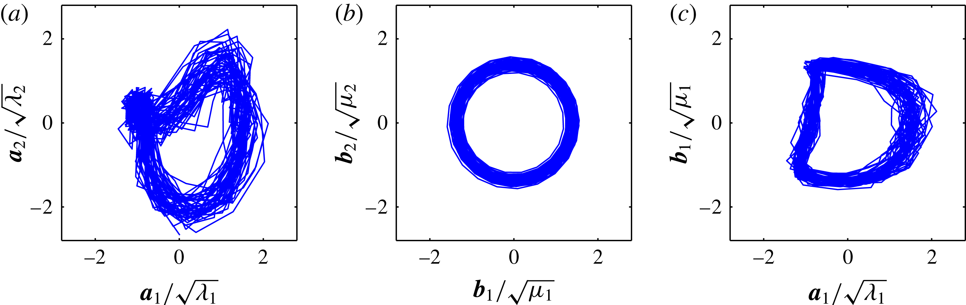
Phase portraits of first temporal coefficients from (a) POD, (b) SPOD and (c) both methods against each other.

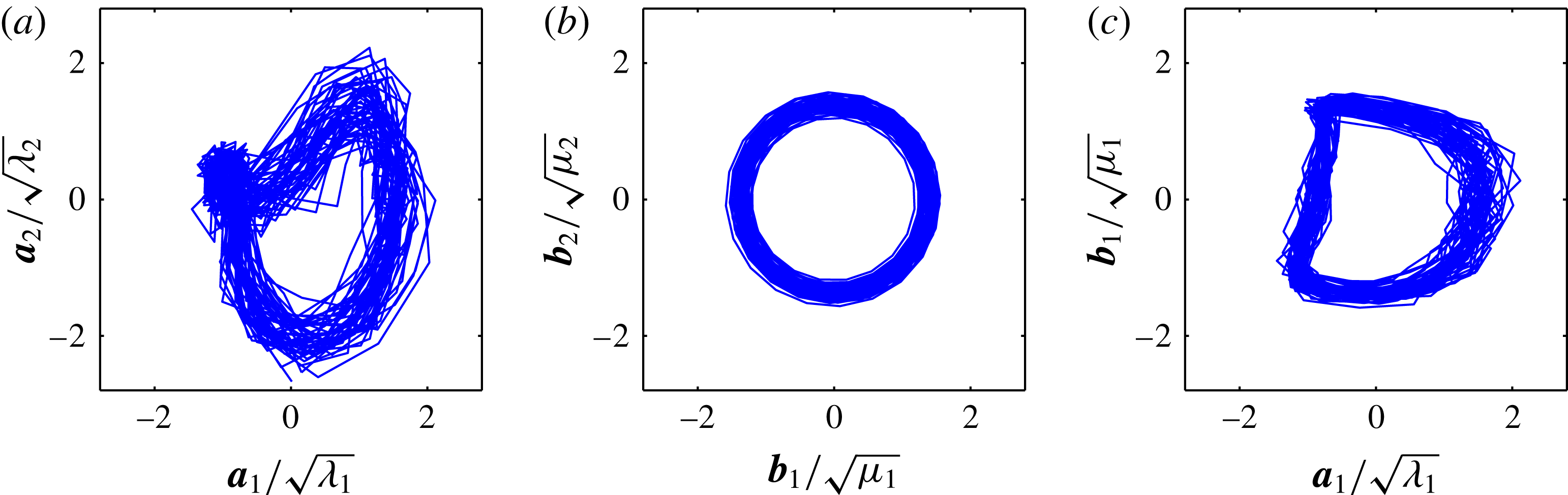
For the fluidic oscillator, the DFT modes are nearly as accurate as those derived with the SPOD. The advantages of the SPOD are more obvious for less mono-frequent flow dynamics (see the previous examples). However, an additional advantage of the SPOD over the DFT is that it provides a reliable estimate of the oscillatory phase by accounting for the frequency jitter. Similar approaches, which also produce satisfactory results for the current case, are described by Ostermann et al. (Reference Ostermann, Woszidlo, Gaertlein, Nayeri and Paschereit2015a ), but again, the scope of SPOD is beyond this particular application. Figure 16(a,b) shows the phase portraits (Lissajous figures) of the temporal coefficients of the two most energetic POD ( $\boldsymbol{a}_{i}$ ) and SPOD ( $\boldsymbol{b}_{i}$ ) modes, respectively. The trajectory of the POD coefficients does not follow a clear circle that would indicate the limit cycle. It rather follows a third of a circle and then collapses at one point. The coefficient of the SPOD modes follows a clear circle and the instantaneous phase and instantaneous frequency can consistently be deduced. A comparison of the first mode coefficient from both methods is shown in figure 16(c). It reveals that half of the period is cut out for the POD ( $\boldsymbol{a}_{1}$ ). This corresponds to the sweeping jet leaving the measurement domain, where the energy-based POD ‘sees’ no jet. The SPOD properly recovers the temporal dynamics over the entire oscillation period. Furthermore, note that the SPOD produces coefficients with smooth temporal dynamics, while the POD coefficients show rather erratic movements. This is particularly important for reduced-order modelling (Luchtenburg et al. Reference Luchtenburg, Günther, Noack, King and Tadmor2009), phase averaging and extended POD (Boree Reference Boree2003). Practically, most of the further processing is eased if there is less noise.