


I. INTRODUCTION
Wireless power transfer (WPT) is increasingly recognized from both academia and industry as a promising solution for the recharging of electronic systems without a physical connection to a power grid [Reference Costanzo1–Reference Li and Mi7].
Among the possible strategies, for applications where the goal is a contactless recharge, the attention has been focused on the use of resonant inductively coupled systems, which allow maximizing the performance for mid-range WPT links [Reference Karalis, Joannopoulos and Soljačić8–Reference Mirbozorgi, Yeon and Ghovanloo12].
In this regard, the case of two inductively coupled resonators has been deeply investigated in the literature. In particular, in [Reference Dionigi, Mongiardo and Perfetti10] the expression of the load impedance which allows maximizing either the power on the load or the efficiency has been derived for a link with assigned parameters. In [Reference Monti, Costanzo, Mastri, Mongiardo and Tarricone13], the equations for designing the optimum link for given values of the source have been reported.
However, although the results reported in the literature demonstrate that for the case of a two-coil link both the power on the load or the efficiency can be maximized by appropriately setting the relevant parameters, the efficiency quickly drops as the transfer distance increases.
Accordingly, the use of multi-resonator systems, where one or more relay resonators are added between the transmitting and the receiving ones, has been proposed as a viable strategy for increasing the transfer distance [Reference Zhang, Hackworth, Fu, Li, Mao and Sun14–Reference Kiani, Jow and Ghovanloo27]. In particular, in [Reference Zhong, Lee and Hui21] the case of a multi-resonator WPT link in a domino arrangement is studied; the analytical expressions of the optimal load and maximum efficiency are derived. It is also experimentally demonstrated the possibility of controlling the power flow in a multi-coil link in various domino arrangements (i.e. straight, curved, circular, and y-shaped). In [Reference Shimada, Ito, Uehara and Ohira28], the case of a multi-resonator link with a single transmitter and multiple receivers is investigated demonstrating that the number of resonators influences the power division ratio of each receiver.
However, the most analyzed case is the one of a link using either three or four resonators. In this regard, in [Reference Kurs, Karalis, Moffatt, Joannopoulos, Fisher and Soljacic22] the case of a four-resonator scheme achieved by using two relay resonators has been experimentally investigated demonstrating the possibility of improving the efficiency with respect to the basic scheme using just two resonators.
In [Reference Lee, Waters, Shi, Park and Smith23], an asymmetrical four-coil link is theoretically investigated. It is shown that for a desired value of the efficiency, there is a maximum operating distance which can be achieved; similarly, for a given operating distance there is a maximum value of the efficiency which can be realized.
In [Reference Kim, Son, Kim and Park24, Reference Zhong, Zhang, Liu and Hui26] the case of a three-resonator link has been analyzed. More specifically, in [Reference Kim, Son, Kim and Park24] the coupled mode theory has been used for deriving the efficiency corresponding to different configurations of the relay element with respect to the transmitting and the receiving resonators; the reported results demonstrate that the use of the intermediate resonator allows improving the efficiency even in the case where it is perpendicularly arranged with respect to the two-resonator link.
Similarly, in [Reference Lee, Kiani and Ghovanloo25] the advantages of a three-coil link are exploited in the context of medical implants. The idea suggested in [Reference Zhong, Zhang, Liu and Hui26] is to use the relay resonator to shift the current stress from the transmitting resonator to the relay element in such a way to improve the magnetic coupling with the receiving coil.
In [Reference Kiani, Jow and Ghovanloo27], based on the reflected load theory, a design procedure for maximizing the efficiency of a link using three and four resonators has been proposed. The performance of the network is described in terms of the two common figures of merit usually adopted for the analysis of WPT links, namely the power transfer efficiency and the active power delivered to the load.
According to the theoretical results achieved for the power on the load and the efficiency of these two schemes, the authors conclude that the three-coil configuration provides the best compromise for the achievable performance in terms of power on the load and efficiency.
This discussion is further deepened in the present paper, where an alternative approach is proposed for solving the same problem. In more detail, the case of a three-resonator link is considered; as in [Reference Kiani, Jow and Ghovanloo27], the three-resonator link is described as a lossy linear two-port network and the relay element is treated as a further degree of freedom of the system, which can be used to optimize the performance. With respect to the analysis proposed in [Reference Kiani, Jow and Ghovanloo27], in the present paper, the gain definitions usually adopted in the context of two-port active networks are used for describing the network behavior. It is shown that this approach is completely equivalent to the description of the network based on the power transfer efficiency and active power on the load. However, the use of three gain definitions that are well established and consolidated in the literature has two main advantages: (1) it eliminates possible ambiguity related to the definition of the variables of interest in the efficiency calculation; (2) it simplifies the calculation and the optimization of the figures of merit of interest. In fact, the three gain definitions adopted in the present paper are usually available in common circuital simulators.
The relevant design equations for the best configuration of the relay element are derived; the best design is expressed in terms of closed form equations of the coupling coefficients of the relay element with the transmitting and the receiving resonators. It is shown that the three-resonator scheme does not allow the analytical maximization of all the figures of merit that could be of interest in the WPT context.
The paper is organized as follows: in Section II, the relevant gain definitions are introduced; in Section III, the definition of conjugate image impedances of a two-port network is briefly recalled and the conditions for maximizing the gains of the network are given and discussed. In Section IV, the analyzed problem is introduced and analytical formulas are derived for the solutions of interest. Later on, in Section V, the theory is validated through circuital simulations; finally, conclusions are drawn in Section VI.
II. GAIN DEFINITIONS FOR TWO-PORT NETWORKS
A two-port network, realized either without relay elements or with one or more relay elements, is advantageously described by gain functions. The latter description is commonly used for amplifiers and can naturally be employed also in the context of WPT. In this section, after a brief definition of the relevant quantities, the most commonly used gain definitions are introduced.
It is assumed that the two-port network realizing WPT is known and a description is available in terms, e.g., of its impedance parameters
 $$z_{ij} = r_{ij} + jx_{ij}{\kern 1pt} $$
with (i, j) = 1, 2. It is also assumed that the input and output ports are connected to a sinusoidal voltage generator V G with internal impedance Z G = R G + jX G , and to a load impedance Z L = R L + jX L , respectively.
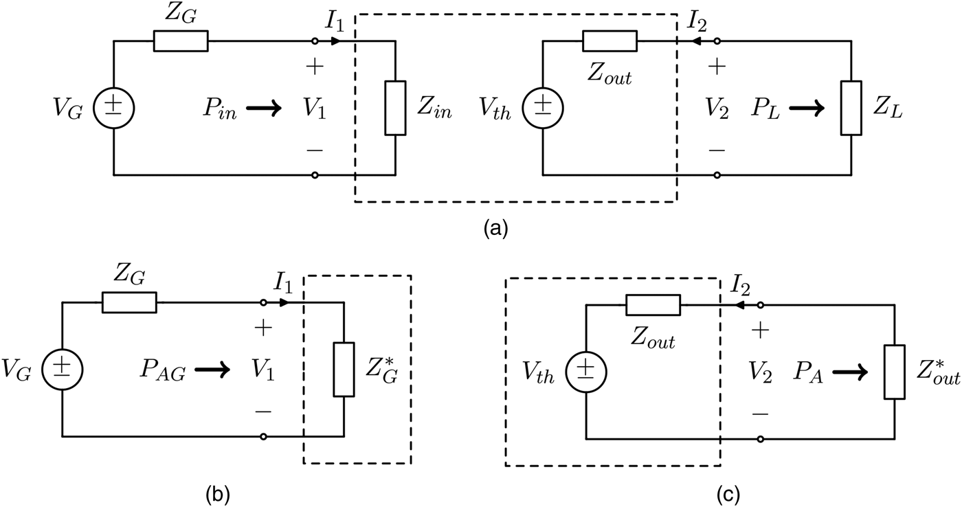
It order to derive the gain functions, it is convenient to represent the two-port network by the Thévenin equivalent circuit depicted in Fig. 1. To this end, the current I 2 on the secondary side is first derived as:
 $$I_2 = - \displaystyle{{z_{21}} \over {z_{22} + Z_L}}I_1{\kern 1pt}, $$
which allows to obtain the following expression for the input impedance:
 $$Z_{in} = R_{in} + j{\kern 1pt} X_{in} = \displaystyle{{V_1} \over {I_1}} = z_{11} - \displaystyle{{z_{12}z_{21}} \over {z_{22} + Z_L}}{\kern 1pt}. $$
(a) Equivalent circuit of a two-port network with Thévenin representation. (b) Definition of the available generator power P AG . (c) Definition of the available output power P A .

The voltage on the secondary side may be then written as:
 $$V_2 = \left( {z_{22} - \displaystyle{{z_{12}z_{21}} \over {z_{11} + Z_G}}} \right)I_2 + \displaystyle{{z_{21}} \over {z_{11} + Z_G}}V_G{\kern 1pt}, $$
which provides the following expression when the generator is short circuited:
 $$Z_{out} = \left. {\displaystyle{{V_2} \over {I_2}}} \right \vert _{V_G = 0} = z_{22} - \displaystyle{{z_{12}z_{21}} \over {z_{11} + Z_G}}{\kern 1pt}. $$
Finally, the Thévenin equivalent voltage is readily obtained as:
 $$V_{th} = \left. {V_2} \right \vert _{I_2 = 0} = \displaystyle{{z_{21}} \over {z_{11} + Z_G}}V_G{\kern 1pt}. $$
Referring to Fig. 1, which illustrates the powers of interest, in the following part of this section, the relevant gain definitions will be introduced.
A) Power gain
The power gain is defined as the ratio between the power delivered to the load and the input power to the two-port network:
 $$G_P = \displaystyle{{P_L} \over {P_{in}}}{\kern 1pt}. $$
The input power is readily evaluated as:
 $$P_{in} = \displaystyle{1 \over 2}R_{in} \vert I_1 \vert ^2,$$
and the output power is given by:
 $$P_L = \displaystyle{1 \over 2}R_L \vert I_2 \vert ^2{\kern 1pt}. $$
The power gain can therefore be expressed as:
 $$G_P = \displaystyle{{R_L} \over {R_{in}}}\left \vert {\displaystyle{{I_2} \over {I_1}}} \right \vert ^2 = \displaystyle{{R_L} \over {R_{in}}}\left \vert {\displaystyle{{z_{21}} \over {z_{22} + Z_L}}} \right \vert ^2.$$
It is noted that G P depends on the load impedance Z L , but does not depend on the generator impedance Z G . In addition, in the WPT context, the power gain is often identified with the efficiency η [Reference Kiani, Jow and Ghovanloo27].
B) Available gain
Another gain expression is the available power gain, which is defined as the ratio between the maximum available load power P A and the available input power P AG :
 $$G_A = \displaystyle{{P_A} \over {P_{AG}}}{\kern 1pt}. $$
The available input power P AG is given by:
 $$P_{AG} = \displaystyle{{ \vert V_G \vert ^2} \over {8R_G}}{\kern 1pt}, $$
while the maximum available load power P A is:
 $$P_A = \displaystyle{{ \vert V_{th} \vert ^2} \over {8R_{out}}}{\kern 1pt}. $$
Hence, their ratio provides:
 $$G_A = \displaystyle{{R_G} \over {R_{out}}}\left \vert {\displaystyle{{V_{th}} \over {V_G}}} \right \vert ^2 = \displaystyle{{R_G} \over {R_{out}}}\left \vert {\displaystyle{{z_{21}} \over {z_{11} + Z_G}}} \right \vert ^2{\kern 1pt}. $$
It can be noted that the available gain is only related to the generator impedance, and does not depend on the load impedance.
C) Transducer gain
The transducer gain of a two-port network is defined by the relation:
 $$G_T = \displaystyle{{P_L} \over {P_{AG}}}.$$
By deriving I 2 as a function of V G :
 $$I_2 = \displaystyle{{V_{th}} \over {Z_{out} + Z_L}} = \displaystyle{{z_{21}V_G} \over {(z_{11} + Z_G)(z_{22} + Z_L) - z_{12}z_{21}}}$$
and replacing this expression in (9), one obtains:
 $$G_T = \displaystyle{{4 \vert z_{21} \vert ^2R_GR_L} \over { \vert (z_{11} + Z_G)(z_{22} + Z_L) - z_{12}z_{21} \vert ^2}}{\kern 1pt}. $$
This expression shows that G T depends both on Z G and Z L .
From the definition of G
T
given in (15), it can be observed that, if the available power is fixed, maximizing the transducer gain is equivalent to maximize the power on the load P
L
. In fact, G
T
is quantitatively coincident with the power delivered to the load for
 $P_{AG} = 1{\kern 1pt} {\rm W}$
. It should also be noted that, in order to keep P
AG
constant, if R
G
is varied, V
G
has to be varied accordingly, as it happens when a matching network is inserted between the generator and the input port.
This shows that the two approaches usually adopted in the WPT context (i.e. the one aiming at maximizing the efficiency of the link and the one aiming at maximizing the power on the load) are equivalent to maximize either G P or G T .
III. CONJUGATE IMAGE IMPEDANCES OF A TWO-PORT NETWORK AND GAINS MAXIMIZATION
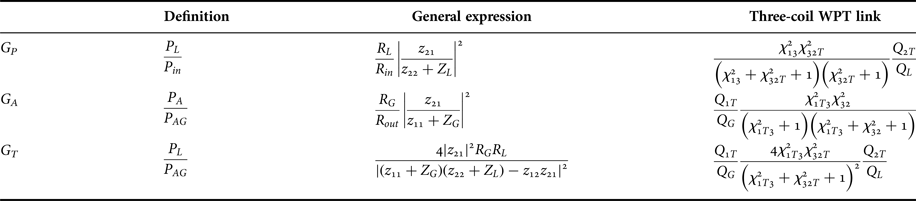
In this section, the conditions for maximizing the gains defined in Table 1 will be discussed. To this end, it is useful to recall the definition of conjugate image impedances of a two-port network [Reference Monti, Costanzo, Mastri and Mongiardo29, Reference Roberts30].
Gain definitions and expressions.

A) Conjugate image impedances
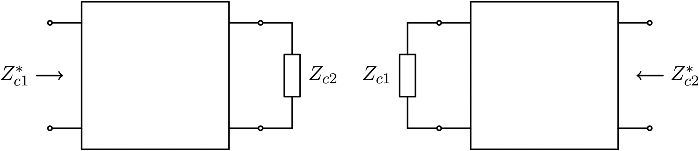
The conjugate image impedances of a two-port network, Z
c1 and Z
c2, are defined as in Fig. 2. When port 2 is terminated on Z
c2, the input impedance seen from port 1 is the complex conjugate of Z
c1 (i.e.
 $Z_{c1}^* $
); similarly, when port 1 is terminated on Z
c1, the input impedance seen from port 2 is the complex conjugate of Z
c2 (i.e.
 $Z_{c2}^* $
). The conjugate image impedances are an intrinsic property of the two-port network and, by using the terms of the impedance matrix, can be expressed as [Reference Roberts30]:
 $$Z_{c1} = R_{c1} + jX_{c1} = r_{11}(\theta _r + j\theta _x) - jx_{11},$$
 $$Z_{c2} = R_{c2} + jX_{c2} = r_{22}(\theta _r + j\theta _x) - jx_{22},$$
Conjugate image impedances as defined in [Reference Roberts30].

where the following definitions have been used:
 $$\theta _r = \sqrt {\left( {1 - \displaystyle{{r_c^2} \over {r_{11}r_{22}}}} \right)\left( {1 + \displaystyle{{x_c^2} \over {r_{11}r_{22}}}} \right)}, $$
 $$\theta _x = \displaystyle{{r_cx_c} \over {r_{11}r_{22}}}, $$
 $$r_c = {\mathop{\rm Re}\nolimits} \left\{ {\sqrt {z_{12}z_{21}}} \right\},$$
 $$x_c = {\mathop{\rm Im}\nolimits} \left\{ {\sqrt {z_{12}z_{21}}} \right\}{\kern 1pt}. $$
It is worth observing that in the case where the terms of the impedance matrix are real quantities (i.e. the terms x ij = 0, (i, j) = 1, 2), the complex conjugate image impedances become purely resistive quantities, and are referred to as image resistances. Another particular case, which is frequently encountered in the WPT context, where Z c1 and Z c2 are purely resistive, is that where z 11 and z 22 are real, while z 12 and z 21 are purely imaginary.
B) Maximization of the gains for a generic two-port network
According to the definitions given in Table 1, it can be shown that:
-
• the power gain G P is independent of Z G , while it depends on Z L and is maximized for Z L = Z c2;
-
• the available gain G A is independent of Z L , while it depends on Z G and is maximized for Z G = Z c1.
As per the transducer gain G T , since
 $$\eqalign{& P_L \le P_A, \cr & P_{in} \le P_{AG},} $$
it results
 $$\eqalign{& G_T \le G_P, \cr & G_T \le G_A.} $$
In particular, it can be noted that:
-
• G T = G P if the power-matching condition
 $Z_G = Z_{in}^* $
is realized at the input port;
-
• G T = G A if the power-matching condition
$Z_L = Z_{out}^* $
is realized at the output port; -
• G T = G P = G A if the power-matching condition is realized at both the input and the output ports, which requires Z G = Z c1 and Z L = Z c2.


Hence, it can be concluded that:
-
• if Z G (or Z L ) is fixed, the maximum value of G T is obtained for
$Z_L = Z_{out}^* $
(or
$Z_G = Z_{in}^* $
); -
• if both Z G and Z L can be optimized, the maximum values of G T is obtained for Z G = Z c1 and Z L = Z c2.


The previous discussion also shows that the maximum of G P with respect to (w.r.t.) Z L , the maximum of G A w.r.t. Z G , and the maximum of G T w.r.t. Z G and Z L are equal. In the following their common value will be denoted by G M .
IV. WPT WITH ONE RELAY ELEMENT
A) Problem description
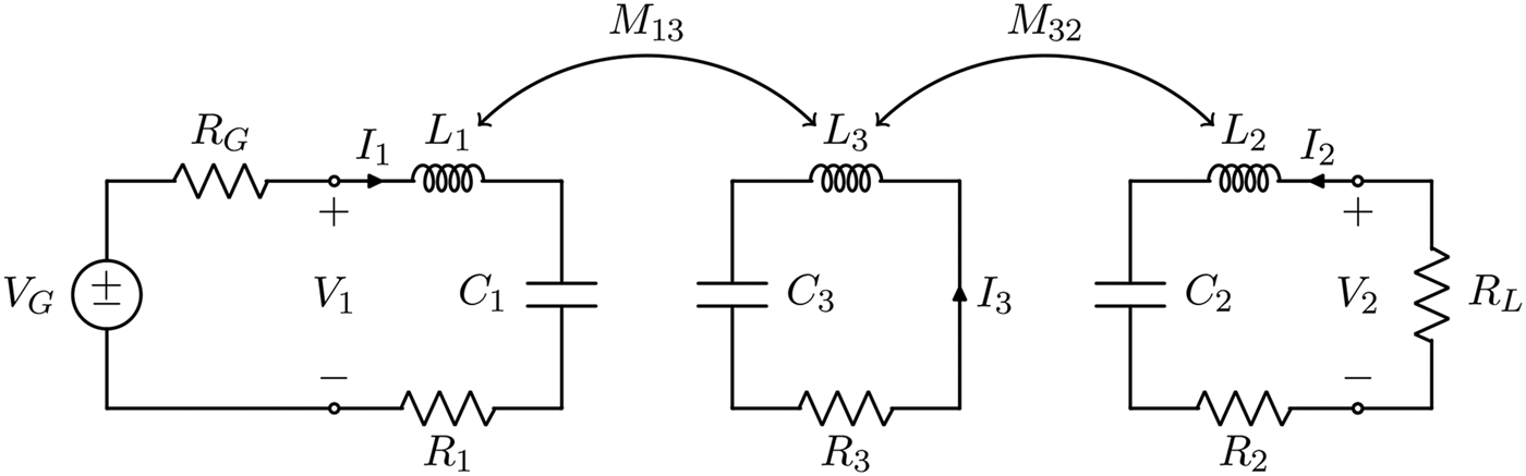
The problem analyzed in this paper is schematically represented in Fig. 3. The case of a resonant inductive WPT link with a relay element is considered. It is assumed that the link is driven by a sinusoidal voltage generator with angular frequency ω 0 and internal resistance R G , and that it is connected to a purely resistive load R L .
Schematic of the WPT link with one relay element.

In the following, the transmitting (TX) resonator is denoted by 1, the receiving resonator (RX) by 2, the relay resonator, placed between the TX and the RX resonators, is denoted by 3. It is assumed that the three coils are synchronous and resonate at the angular frequency ω 0.
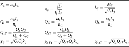
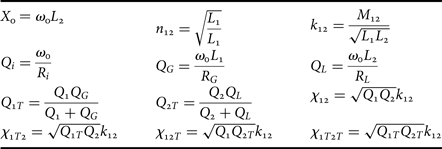
The symbols defined in Table 2 are used for the analysis. For each resonator, the loss resistance is denoted by R
i
and the unloaded quality factor by Q
i
. The external quality factors of the TX and RX resonators are indicated by Q
G
and Q
L
, respectively, while the corresponding loaded quality factors are indicated by Q
1T
and Q
2T
. The coupling coefficient between coils i and j is denoted by k
ij
; it is assumed that only adjacent coils are coupled, i.e. only k
13 and k
32 are different from zero, while k
12 = 0. The reactance of the inductor at the receiving side,
 $X_0 = \omega _0{\kern 1pt} L_2$
, is used for normalization. The parameters n
ij
represent the transformation ratios. Finally, the symbols χ
ij
, χ
1T3, and χ
32T
are also introduced, in order to alleviate the notation.
Definitions.

In this paper, the following problems will be considered and solved.
-
• CASE A – Assuming that the parameters of the link (and therefore the couplings k 13 and k 32) are given, find the optimal values of R G and R L for maximizing the gains of the network.
-
• CASE B – Assuming that the load and the generator impedances are given, try to maximize the gains of the two-port network by acting either on the receiving side (i.e. by optimizing k 32) or on the transmitting side (i.e. by optimizing k 13).
All the above cases may include, or may not, a communication between the TX and the RX in the optimization phase.
1) IMPEDANCE MATRIX OF A THREE-COIL LINK
At the operating angular frequency ω 0, the equations for the three-coil link are
 $$\eqalign{& V_1 = R_1I_1 + j\omega _0M_{13}I_3, \cr & V_2 = R_2I_2 + j\omega _0M_{32}I_3, \cr & 0 = j\omega _0M_{13}I_1 + j\omega _0M_{32}I_2 + R_3I_3{\kern 1pt}.} $$
From (26), making use of the definition reported in Table 2, the following expressions can be derived for the parameters of the link impedance matrix:
 $$\eqalign{& z_{11} = r_{11} = \displaystyle{{X_0n_{12}^2} \over {Q_1}}\left( {\chi _{13}^2 + 1} \right), \cr & z_{12} = z_{21} = r_{12} = \displaystyle{{X_0n_{12}} \over {\sqrt {Q_1Q_2}}} \chi _{13}\chi _{32}, \cr & z_{22} = r_{22} = \displaystyle{{X_0} \over {Q_2}}\left( {\chi _{32}^2 + 1} \right){\kern 1pt}.} $$
It can be noted that all the elements of the impedance matrix are real.
2) INPUT AND OUTPUT RESISTANCES
Since the terminating impedances are assumed to be purely resistive, also the input and output impedances of the three-coil link are real. From (27), by means of (3) and (5), their expressions can be derived as
 $$R_{in} = \displaystyle{{X_0n_{12}^2} \over {Q_1}}\displaystyle{{\chi _{13}^2 + \chi _{32T}^2 + 1} \over {\chi _{32T}^2 + 1}},$$
 $$R_{out} = \displaystyle{{X_0} \over {Q_2}}\displaystyle{{\chi _{1T3}^2 + \chi _{32}^2 + 1} \over {\chi _{1T3}^2 + 1}}{\kern 1pt}. $$
3) CONJUGATE IMAGE IMPEDANCES
As previously stated, since all the terms of the impedance matrix of a three-coil WPT link are purely real, the conjugate image impedances are simply the image resistances, and can be derived by (18) and (19) as:
 $$Z_{c1} = R_{i1} = \displaystyle{{X_0n_{12}^2} \over {Q_1}}\sqrt {\displaystyle{{\left( {\chi _{13}^2 + 1} \right)\left( {\chi _{13}^2 + \chi _{32}^2 + 1} \right)} \over {\chi _{32}^2 + 1}}}, $$
 $$Z_{c2} = R_{i2} = \displaystyle{{X_0} \over {Q_2}}\sqrt {\displaystyle{{\left( {\chi _{32}^2 + 1} \right)\left( {\chi _{13}^2 + \chi _{32}^2 + 1} \right)} \over {\chi _{13}^2 + 1}}} {\kern 1pt}. $$
4) POWER GAIN, AVAILABLE GAIN, AND TRANSDUCER GAIN
The expressions of the gains for a three-coil WPT link can be calculated by substituting (27) in the general expressions summarized in Table 1. For the power gain, the following expression can be obtained:
 $$G_P = \displaystyle{{\chi _{13}^2 \chi _{32T}^2} \over {\left( {\chi _{13}^2 + \chi _{32T}^2 + 1} \right)\left( {\chi _{32T}^2 + 1} \right)}}{\kern 1pt} \displaystyle{{Q_{2T}} \over {Q_L}}.$$
The expression of the available gain is:
 $$G_A = \displaystyle{{Q_{1T}} \over {Q_G}}{\kern 1pt} \displaystyle{{\chi _{1T3}^2 \chi _{32}^2} \over {\left( {\chi _{1T3}^2 + 1} \right)\left( {\chi _{1T3}^2 + \chi _{32}^2 + 1} \right)}}.$$
Finally, the expression of the transducer gain is:
 $$G_T = \displaystyle{{Q_{1T}} \over {Q_G}}{\kern 1pt} \displaystyle{{4\chi _{1T3}^2 \chi _{32T}^2} \over {{\left( {\chi _{1T3}^2 + \chi _{32T}^2 + 1} \right)}^2}}{\kern 1pt} \displaystyle{{Q_{2T}} \over {Q_L}}.$$
B) CASE A: optimal load impedance for a three-coil link
According to the results obtained for a generic two-port network, the power gain G P is maximized for R L = R i2 given by (31), the available gain G A is maximized for R G = R i1 given by (30), and the transducer gain G T is maximized for R G = R i1 and R L = R i2. When the previous conditions are satisfied, the tree gains assume the same maximum value, which can be expressed as
 $$G_M = \displaystyle{{{\left[ {\sqrt {\chi _{13}^2 + \chi _{32}^2 + 1} - \sqrt {\left( {\chi _{13}^2 + 1} \right)\left( {\chi _{32}^2 + 1} \right)}} \right]}^2} \over {\chi _{13}^2 \chi _{32}^2}}. $$
As per the transducer gain, if the load resistance is fixed, its maximum w.r.t. R G is obtained when R G = R in given by (28), and is equal to G P given by (32). Analogously, if the generator resistance is fixed, the maximum of G T w.r.t. R L is obtained when R L = R out given by (29), and is equal to G A given by (33).
C) CASE B: optimizing a three-coil link when the source and the load are given
In most cases of practical interest, the source and the load are given and can not be freely selected to maximize the performance of the link.
In these cases, the parameters of the link have to be used for maximizing the performance. In this regard, a viable solution is to act on the couplings of the relay element with the primary and the secondary resonators. In particular, one of the two couplings could be used for satisfying the requirement on the transfer distance and the other one to maximize the performance of the link. Accordingly, two different scenarios are of interest:
-
• it is possible to use k 13 to satisfy the requirement on the transfer distance and to act on the receiving side by modifying the magnetic coupling k 32 to maximize the performance;
-
• it is possible to use k 32 to satisfy the requirement on the transfer distance and to act on the transmitting side by modifying the magnetic coupling k 13 to maximize the performance.
1) OPTIMIZING THE COUPLING BETWEEN RELAY AND RECEIVING COIL
Assuming that k 13 is set according to the requirement on the distance to be covered by the link, the possibility to act on k 32 to maximize the performance in terms of one of the three gains of the network is investigated.
Power gain
The value of k 32 which maximizes G P (i.e. the efficiency of the link) is obtained by equating to zero the derivative of (32) w.r.t. k 32:
 $$k_{32}^{GP} = \displaystyle{{\root 4 \of {\chi _{13}^2 + 1}} \over {\sqrt {Q_{2T}Q_3}}}. $$
It can be easily verified that the results expressed in (36) is equivalent to that given in equation (25) of [Reference Kiani, Jow and Ghovanloo27]. For
 $k_{32} = k_{32}^{GP} $
the value of G
P
becomes
 $$G_{P32}^M = \displaystyle{{{\left( {1 - \sqrt {\chi _{13}^2 + 1}} \right)}^2} \over {\chi _{13}^2}} \displaystyle{{Q_{2T}} \over {Q_L}}.$$
This solution is physically realizable for
 $k_{32}^{GP} \lt 1$
, i.e.:
 $$Q_{2T} \gt \displaystyle{{\sqrt {\chi _{13}^2 + 1}} \over {Q_3}}.$$
According to (38), it is possible to maximize G P by acting on the receiving side only if Q L is not too small, this being equivalent to require that R L is smaller than a value which depends on k 13. In more detail, the upper value of R L decreases with k 13; hence, for a given R L the maximization of G P as function of k 32 may become unfeasible for high values of k 13.
Additionally, it can be verified that in (37) the first factor is the maximum value of G
P
for the two-coil link formed by resonators 1 and 3 (see the Appendix), while the second factor is the efficiency of resonator 2. This means that optimizing G
P
by setting
 $k_{32} = k_{32}^{GP} $
is equivalent to use resonator 2 for realizing a matching network, which transforms the load R
L
into the reflected resistance
 $$R_{R,out} = \displaystyle{{{\left( {\omega _0M_{32}} \right)}^2} \over {R_L + R_2}} = \displaystyle{{X_0n_{32}^2} \over {Q_3}}\sqrt {\chi _{13}^2 + 1} {\kern 1pt}, $$
corresponding to the image resistance R i2 of the link formed by resonators 1 and 3.
Available gain
The derivative of the available gain w.r.t. k 32 is zero only for k 32 = 0, which means that it is not feasible to analytically maximize also the available gain for a given k 13: G A keeps growing as k 32 increases.
Transducer gain
The value of k 32, which maximizes the transducer gain, can be calculated by equating to zero the derivative of (34) w.r.t. k 32:
 $$k_{32}^{GT} = \sqrt {\displaystyle{{\chi _{1T3}^2 + 1} \over {Q_{2T}Q_3}}}. $$
When k 32 is set according to (40), G T assumes the value:
 $$G_{T32}^M = \displaystyle{{Q_{1T}} \over {Q_G}}\displaystyle{{\chi _{1T3}^2} \over {\chi _{1T3}^2 + 1}}\displaystyle{{Q_{2T}} \over {Q_L}}.$$
It is worth observing that, by measuring the power on the load, it is possible to perform experimentally this optimization without communication with the transmitting side. The value of k
32 expressed in (40) is physically realizable (i.e.
 $k_{32}^{GT} \lt 1$
) for:
 $$Q_{2T} \gt \displaystyle{{\chi _{1T3}^2 + 1} \over {Q_3}}.$$
Accordingly, by acting on the receiving side, it is possible to maximize G T for values of Q 2T satisfying (42), this corresponding to impose an upper limit to R L . As evident from (42), the upper limit on R L depends on k 13 and lowers for increasing values of k 13. Consequently, for a given R L the solution may become unfeasible for high values of k 32.
It can also be observed that the expression (41) of
 $G_{T32}^M $
can be interpreted as the product of the maximum transducer gain of the two-coil link formed by resonators 1 and 3 w.r.t. its load resistance (see the Appendix), and the efficiency of resonator 2.
This means that the coupled resonators 2 and 3 act as a lossy matching network, which transforms the load resistance R L into the reflected resistance:
 $$R_{R,out} = \displaystyle{{{\left( {\omega _0M_{32}} \right)}^2} \over {R_L + R_2}} = \displaystyle{{X_0n_{32}^2} \over {Q_3}}\left( {\chi _{1T3}^2 + 1} \right),$$
which is equal to the output resistance of the two-coil link formed by resonators 1 and 3. Hence
 $k_{32}^{GT} $
realizes the power-matching condition at the output port of the link formed by coils 1 and 3. However, it can be noted that in these conditions, the output port impedance of the three-coil link is not matched. In fact, for
 $k_{32} = k_{32}^{GT} $
it results
 $$R_{out} = X_0\left( {\displaystyle{2 \over {Q_2}} + \displaystyle{1 \over {Q_L}}} \right) = R_L + 2R_2{\kern 1pt}, $$
hence R out becomes equal to the load resistance only if the RX resonator losses tend to zero. Nevertheless, the non-optimal power transfer at the output port is compensated by the optimal transducer gain of the first two-coil link. As a result, in these conditions, the best three-coil link which can be realized by simply varying k 32 is obtained.
2) OPTIMIZING THE COUPLING BETWEEN RELAY AND TRANSMITTING COIL
In this case, it is assumed that k 32 is set to satisfy the requirement on the distance to be covered by the link, and the possibility to use k 32 to maximize the performance in terms of the three gains of the two-port network is investigated.
Power gain
The derivative of the power gain w.r.t. k 13 is zero only for k 13 = 0, hence G P keeps growing as k 13 increases. As a consequence, it is not feasible to maximize G P by acting on the transmitting side, while keeping constant k 32.
Available gain
For a given value of k 32, the available gain G A can be optimized for
 $$k_{13}^{GA} = \displaystyle{{\root 4 \of {\chi _{32}^2 + 1}} \over {\sqrt {Q_{1T}Q_3}}} {\kern 1pt}. $$
The corresponding maximum value of G A is:
 $$G_{A14}^M = \displaystyle{{Q_{1T}} \over {Q_G}}\displaystyle{{{\left( {1 - \sqrt {\chi _{32}^2 + 1}} \right)}^2} \over {\chi _{32}^2}} {\kern 1pt}. $$
The solution expressed in (46) is physically realizable for
 $k_{13}^{GA} \lt 1$
, which requires:
 $$Q_{1T} \gt \displaystyle{{\sqrt {\chi _{32}^2 + 1}} \over {Q_3}}.$$
Hence, similarly to G
T
with varying k
32, it is possible to maximize G
A
by acting on the transmitting side only if R
G
is not too large. The upper value of R
G
decreases with k
32 and
 $k_{13}^{GA} $
may become physically not realizable for high values of k
32.
It is worth noticing that in (46), the first factor is the efficiency of the resonator 1, while the second factor is the maximum value of G A for the two-coil link formed by resonators 3 and 2 (see the Appendix for the expression of G A for a two-coil link).
Accordingly, it can be seen that for
 $k_{13} = k_{13}^{GA} $
the coupled resonators 1 and 2 transform the generator resistance R
G
into the reflected resistance
 $$R_{R,in} = \displaystyle{{{\left( {\omega _0M_{13}} \right)}^2} \over {R_G + R_1}} = \displaystyle{{X_0n_{32}^2} \over {Q_3}}\sqrt {\chi _{32}^2 + 1}, $$
which is equal to the image resistance R i1 of the link formed by resonators 2 and 3.
Transducer gain
The derivative of (34) with respect to k 13 is zero for
 $$k_{13}^{GT} = \sqrt {\displaystyle{{\chi _{32T}^2 + 1} \over {Q_{1T}Q_3}}}, $$
giving the following value of the transducer gain
 $$G_{T13}^M = \displaystyle{{Q_{1T}} \over {Q_G}}\displaystyle{{\chi _{32T}^2} \over {\chi _{32T}^2 + 1}}\displaystyle{{Q_{2T}} \over {Q_L}}.$$
It is noted that, also in this case, the optimization can be performed without communication with the receiving side. In fact, for constant values of k 32 and R L , G P is also constant and, according to (34), in order to maximize G T it is necessary to maximize P in .
The feasibility of the solution expressed in (49) imposes:
 $$Q_{1T} \gt \displaystyle{{\chi _{32T}^2 + 1} \over {Q_3}}.$$
This means that by acting on the transmitting side, it is possible to maximize G T for values of Q 1T satisfying (51), this being equivalent to impose an upper limit to R G . In more detail, the upper limit on R G depends on k 32 and lowers for increasing values of k 13; hence, for a given value of R L , the possibility of maximizing G T by acting on k 13 depends on k 32.
It is worth noticing that the expression (50) of
 $G_{T,13}^M $
can be interpreted as the product of the efficiency of resonator 1 and the maximum transducer gain of the two-coil link formed by resonators 3 and 2 w.r.t. its load resistance (see the Appendix for the expression of G
T
for a two-coil link).
Accordingly, the coupled resonators 1 and 3 transform the R G into the reflected impedance
 $$R_{R,in} = \displaystyle{{{\left( {\omega _0M_{13}} \right)}^2} \over {R_G + R_1}} = \displaystyle{{X_0n_{32}^2} \over {Q_3}}\left( {\chi _{32T}^2 + 1} \right),$$
which is equal to the input resistance of the link formed by resonators 3 and 2. This means that
 $k_{13}^{GT} $
realizes the power-matching condition at the input port of the link formed by coils 3 and 2. As in the previous case, it can be noted that in these conditions, the input port impedance of the three-coil link is not matched. In fact, for
 $k_{13} = k_{13}^{GT} $
it results
 $$R_{in} = X_0n_{12}^2 \left( {\displaystyle{2 \over {Q_1}} + \displaystyle{1 \over {Q_G}}} \right) = R_G + 2R_1{\kern 1pt}, $$
hence R in becomes equal to the generator resistance only if the TX resonator losses tend to zero.
3) DISCUSSION ON THE RESULTS
The analyses performed in the previous section show that:
-
• By keeping fixed the coupling factor between the transmitter and the relay element k 13, it is possible to vary k 32 to optimize the efficiency (i.e. G P ) and the power on the load (i.e. G T ) provided that the conditions expressed in (38) and in (42) are satisfied, while it is not possible to optimize the available gain G A .
-
• By keeping fixed the coupling factor between the relay element and the receiver k 32, it is possible to vary k 13 to optimize the power on the load and the available gain G A provided that the conditions expressed in (51) and in (47) are satisfied, while it is not possible to optimize the efficiency.
It should be pointed out that, since in neither case it is possible to optimize both the available and the transducer gain, only local maxima of the transducer gain, and consequently of the output power, can be achieved. In order to overcome these limitations, it is appropriate to investigate the behavior of a WPT link with two relay elements.
Additionally, according to the expressions (37), (41), (46), (50) of the maximized gains, it can be concluded that case B is equivalent to consider the problem of the cascade of two links: one with a variable coupling (i.e. the one formed by resonator 3 and either resonator 1 or 2) and one with a fixed coupling (i.e. the one formed by resonator 3 and either resonator 2 or 1). The link with a variable coupling is used as a matching network, where the variable coupling is exploited in order to maximize one of the gains of the link with fixed coupling. Accordingly:
-
• When the goal is to maximize G T , the optimum value of the variable coupling is the one which realizes the power-matching condition at either the input or the output ports of the fixed link.
-
• When the goal is to maximize G A or G P , the optimum value of the variable coupling is the one which realizes, for the fixed link, its conjugate image impedance at either the input (maximization of G A ) or output port (maximization of G P ).
V. NUMERICAL VERIFICATION
In order to verify the theory reported in the previous sections, circuital simulations have been performed with the commercial tool NI AWR design environment. The value assumed for the coils are reported in Table 3 and were taken from [Reference Kiani, Jow and Ghovanloo27] (see Table 2).
Data of the coils.

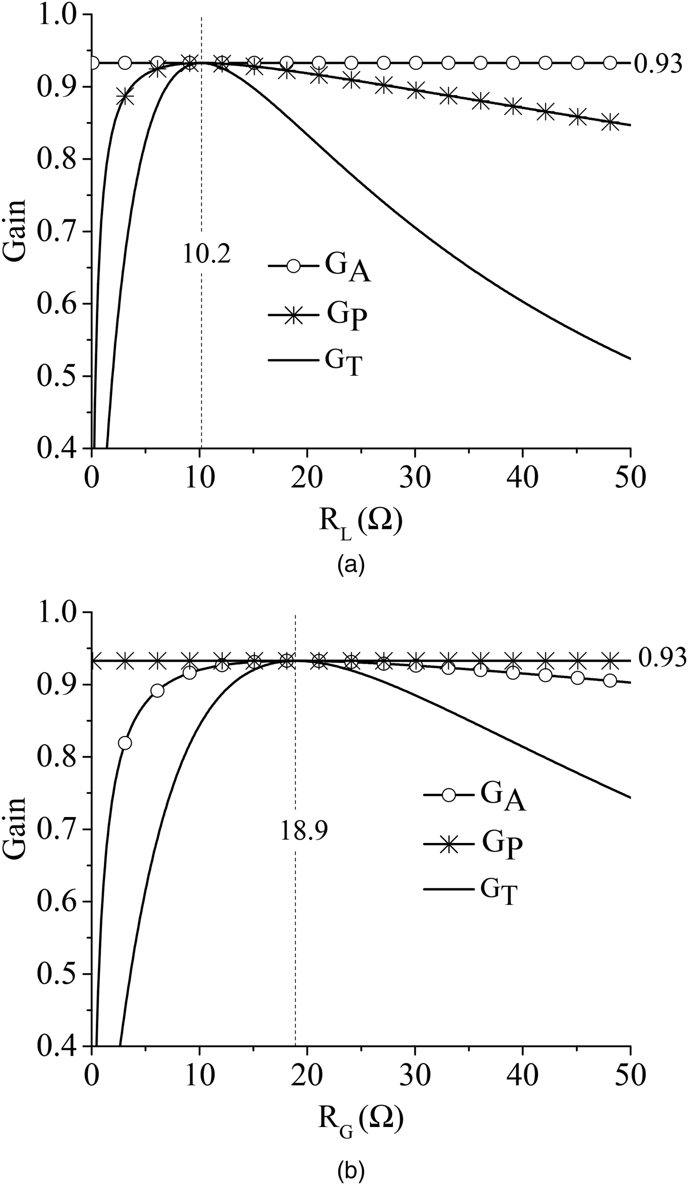
First of all, simulations were performed in order to verify that it is possible to maximize all the three gains by setting R G = R i1 and R L = R i2. To this end, simulations were performed:
-
• by setting
$R_G = R_{i1} = 18.9{\kern 1pt} \Omega $
and by varying R
L
(see Fig. 4a), -
• by setting
$R_L = R_{i2} = 10.2{\kern 1pt} \Omega $
and by varying R
G
(see Fig. 4b).


Results obtained from circuital simulations for G T , G P , and G A by varying: (a) the value of R L for R G = R i1, (b) the value of R G for R L = R i2. The values assumed for k 13 and k 32 are 0.2 and 0.22, respectively.

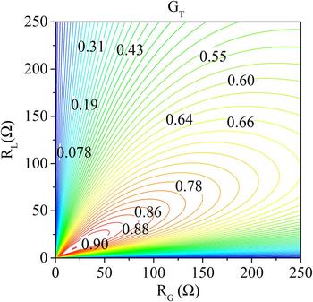
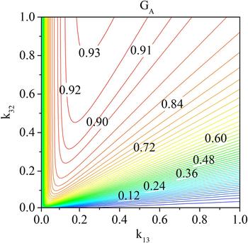
It can be seen that circuital simulations confirm the theory; in fact, the three gains are maximized for R G = R i1 and R L = R i2. It can be also seen that for R G = R i1 and R L = R i2, the gains assume the same value: G T = G A = G P = G M = 0.93. Additionally, as expected, G A is independent of R L while G P is independent of R G . As per G P , the dependence on both R G and R L is highlighted in Fig. 5.
Results obtained from circuital simulations for G T by varying R G and R L . The values assumed for k 13 and k 32 are 0.2 and 0.22, respectively.

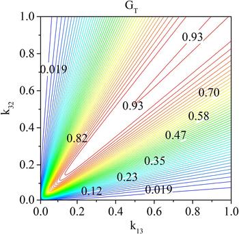
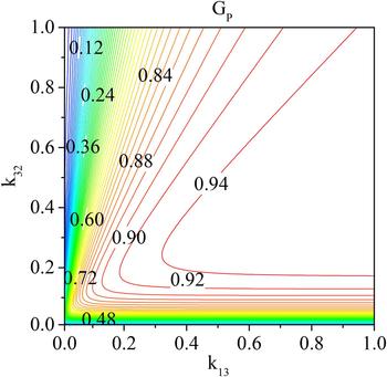
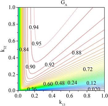
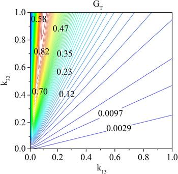
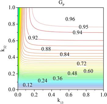
Later on, simulations were performed by varying the values of k 13 and k 32. The results obtained this way for G P , G T , and G A are given in Figs 6–8. According to the theoretical analysis, it can be seen that for a given value of k 13, G P and G T can be maximized by an appropriate selection of the value of k 32, while it can be seen that G A keeps growing as k 32 increases.
Results obtained from circuital simulations for the available gain G
T
by varying the values of k
13 and k
32. The values assumed for R
G
and R
L
are
 $10{\kern 1pt} \Omega $
and
 $5{\kern 1pt} \Omega $
, respectively.

Results obtained from circuital simulations for the available gain G
P
by varying the values of k
13 and k
32. The values assumed for R
G
and R
L
are
 $10{\kern 1pt} \Omega $
and
 $5{\kern 1pt} \Omega $
, respectively.

Results obtained from circuital simulations for the available gain G
A
by varying the values of k
13 and k
32. The values assumed for R
G
and R
L
are
 $10{\kern 1pt} \Omega $
and
 $5{\kern 1pt} \Omega $
, respectively.

In the same figures, it is also evident that by acting on k
13 for a given value of k
23 it is possible to maximize G
T
and G
A
, while G
P
continues to increase as k
13 increases. The same behavior can be observed in Figs 9–11, where the results calculated for
 $R_G = 5{\kern 1pt} \Omega $
and
 $R_L = 200{\kern 1pt} \Omega $
are reported. The intrinsic limits of the three-coil configuration are particularly evident in Fig. 10, where it can be seen that for k
32 lower than 0.2 very low values of G
P
are obtained for any value of k
13. By comparing Figs 7 and 10, it can be also seen that, according to (38), for a given value of k
13 the value of k
32 which allows maximizing G
P
increases with R
L
. In particular, according to (38), for the case analyzed in Fig. 10 (i.e.
 $R_G = 5{\kern 1pt} \Omega $
and
 $R_L = 200{\kern 1pt} \Omega $
), the value of k
32 which allows maximizing G
P
is not physically realizable for k
13 >0.14.
Results obtained from circuital simulations for the available gain G
T
by varying the values of k
13 and k
32.
 $R_G = 5{\kern 1pt} \Omega $
and
 $R_L = 200{\kern 1pt} \Omega $
.

Results obtained from circuital simulations for the available gain G
P
by varying the values of k
13 and k
32.
 $R_G = 5{\kern 1pt} \Omega $
and
 $R_L = 200{\kern 1pt} \Omega $
.

Results obtained from circuital simulations for the available gain G
A
by varying the values of k
13 and k
32. Results obtained for
 $R_G = 5{\kern 1pt} \Omega $
and
 $R_L = 200{\kern 1pt} \Omega $
.

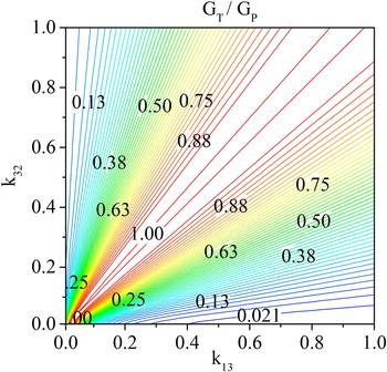
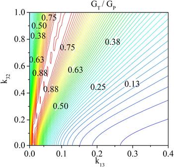
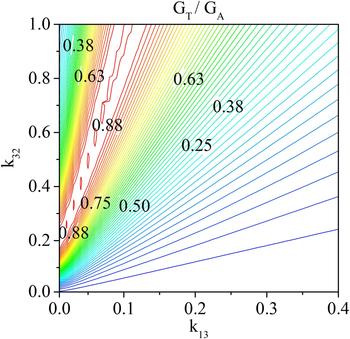
It is worth observing that the ratio between the transducer gain and the power gain is an indicator of the level of matching at the input port of the network with respect to the generator with internal resistance R G ; in fact, G T /G P is the portion of the power available from the generator that is transferred to the network:
 $$\displaystyle{{G_T} \over {G_P}} = \displaystyle{{P_{in}} \over {P_{AG}}}.$$
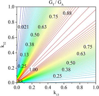
Similarly, the ratio between the transducer gain and the available gain is an indicator of the level of matching at the output port of the network with respect to the load R L ; in fact, G T /G A is the portion of the maximum available load power which is delivered to the given load R L :
 $$\displaystyle{{G_T} \over {G_A}} = \displaystyle{{P_L} \over {P_A}}.$$
The results obtained by circuital simulations are given in Figs 12–15; in more detail, Figs 12 and 13 refer to
 $R_G = 10{\kern 1pt} \Omega $
and
 $R_L = 5{\kern 1pt} \Omega $
, while Figs 14 and 15 refer to
 $R_G = 5{\kern 1pt} \Omega $
and
 $R_L = 200{\kern 1pt} \Omega $
.
Results obtained from circuital simulations for the ratio between the transducer gain G
T
and the power gain G
P
by varying the values of k
13 and k
32. Results obtained for
 $R_G = 10{\kern 1pt} \Omega $
and
 $R_L = 5{\kern 1pt} \Omega $
.

Results obtained from circuital simulations for the ratio between the transducer gain G
T
and the available gain G
A
by varying the values of k
13 and k
32. Results obtained for
 $R_G = 10{\kern 1pt} \Omega $
and
 $R_L = 5{\kern 1pt} \Omega $
.

Results obtained from circuital simulations for the ratio between the transducer gain G
T
and the power gain G
P
by varying the values of k
13 and k
32. Results obtained for
 $R_G = 5{\kern 1pt} \Omega $
and
 $R_L = 200{\kern 1pt} \Omega $
.

Results obtained from circuital simulations for the ratio between the transducer gain G
T
and the available gain G
A
by varying the values of k
13 and k
32. Results obtained for
 $R_G = 5{\kern 1pt} \Omega $
and
 $R_L = 200{\kern 1pt} \Omega $
.

From these figures, it can be seen that the dependence of G T /G P and G T /G A on the couplings k 13 and k 23 is the same calculated for G T ; in fact, in order to maximize the power delivered to the load, it is necessary to maximize both G T /G P and G T /G A .
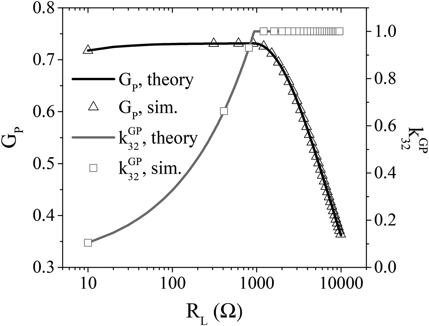
Finally, for the sake of comparison with [Reference Kiani, Jow and Ghovanloo27], in Fig. 16, the results achieved in using k
32 to keep the power gain to its maximum value while the load is varying are reported. The figure shows the data provided by the analytical formulas for
 $k_{32}^{GP} $
as function of the load resistance R
L
; the corresponding G
P
is also reported. It can be easily verified that the results reported in Fig. 16 are in agreement with those reported in Fig. 5b of [Reference Kiani, Jow and Ghovanloo27]. According to (38), by adjusting the value of k
32 it is possible to maintain G
P
to its maximum value for values of R
L
satisfying the following relation:
 $$R_L \lt R_2{\kern 1pt} \left( {\displaystyle{{Q_2{\kern 1pt} Q_3} \over {\sqrt {\chi _{13}^2 + 1}}} - 1} \right),$$
which, for the analyzed case, leads to an upper limit for R
L
of about
 $935{\kern 1pt} \Omega $
. In Fig. 16, the results obtained from circuital simulations and validating the theory are also reported.
Results obtained for
 $k_{32}^{GP} $
and the corresponding G
P
as function of R
L
. The value assumed for k
13 is 0.03. The figure shows a comparison between data provided by the analytical formulas and the results obtained by circuital simulations.

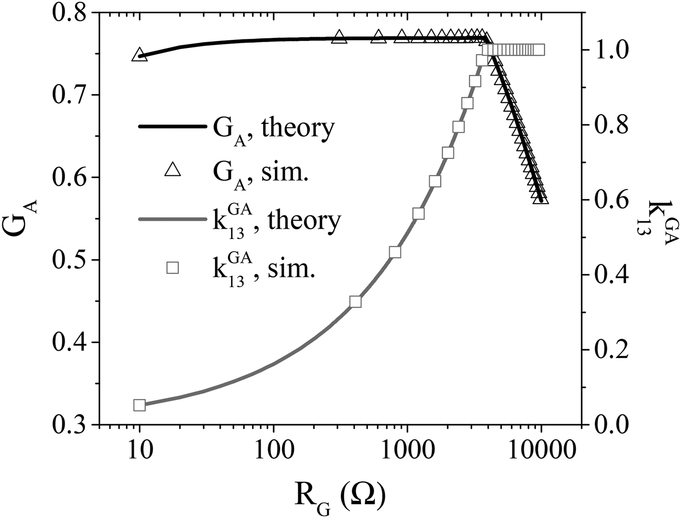
Similar considerations are valid with regard to the use of k
13 to keep the available gain to its maximum value while the generator impedance R
G
is varying. The data calculated from analytical formulas for
 $k_{13}^{GA} $
as function of R
G
are given in Fig. 17 and compared with circuital simulation results.
Results obtained for
 $k_{13}^{GA} $
and the corresponding G
A
as function of R
G
. The value assumed for k
32 is 0.1. The figure shows a comparison between data provided by the analytical formulas and the results obtained by circuital simulations.

According to (47), by varying the value of k 13 it is possible to maintain G A to its maximum value for values of R G below the upper limit expressed by:
 $$R_G \lt R_1{\kern 1pt} \left( {\displaystyle{{Q_1{\kern 1pt} Q_3} \over {\sqrt {\chi _{32}^2 + 1}}} - 1} \right),$$
which, for the present case, is equal to about
 $3821{\kern 1pt} \Omega $
.
VI. CONCLUSION
The problem of magnetic resonant WPT between one transmitter and one receiver coupled through a relay element has been considered from a rigorous network viewpoint. Given the network parameters, the problem of maximizing the performance of the network has been analytically solved. In more detail, the link performance has been described by using the standard gain definitions available for a two-port network: power, available, and transducer gain. It has been shown that the definition usually adopted in the WPT context for the efficiency is equivalent to the power gain of the network and that, for given values of the available power of the generator, maximizing the power on the load is equivalent to maximize the transducer gain.
For the analyzed case, it has been shown that the impedance matrix is purely resistive and, as a consequence, the conjugate image impedances are simply the image resistances. Accordingly, in the case of given parameters of the link it has been shown that it is possible to maximize all the gains by setting the generator and the load impedance equal to the image resistances of the network. As per the case where the load and the source are given, one of the couplings (e.g. the coupling between the transmitter and the relay element or the coupling between the relay element and the receiver) can be set in order to satisfy the requirement on the distance to be covered by the link and the other one can be optimized to maximize one of the three network gains. However, the results reported in this paper demonstrate that the possibility of analytically maximizing the available gain and the power gain depends on which of the two couplings of the relay element, the one with the transmitter or the one with the receiver, is considered as a degree of freedom.
In particular, from analytical formulas and circuital simulations, it has been shown that when the coupling between the transmitter and the relay element is fixed, it is not possible to maximize the available gain G A , which keeps growing for increasing values of the coupling between the relay element and the receiver. Similarly, for a given value of the coupling between the relay element and the receiver, it has been shown that it is not possible to find the absolute maximum of the efficiency (i.e. the power gain G P ). In fact, G P increases for increasing values of the coupling between the relay element and the transmitter.
Since, in order to achieve the maximum transducer gain, and consequently the maximum output power, it is necessary to maximize both the available and the power gain, only a local maximum can be obtained for G T by using just one relay element.
APPENDIX: EXPRESSIONS OF THE GAINS FOR A TWO-COIL WPT LINK
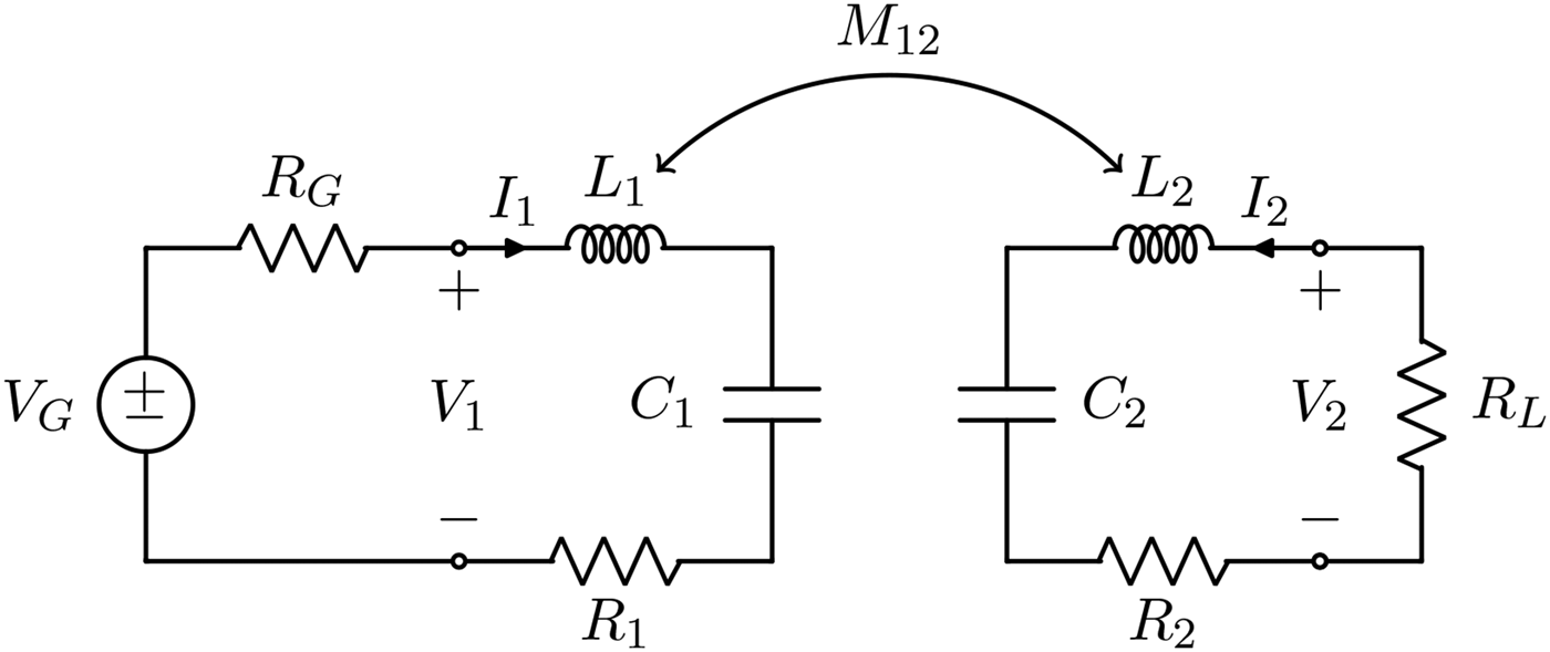
In this section, the expressions of the three gains for a two-coil WPT link are briefly recalled. It is assumed that the link, which is depicted in Fig. 18, is fed by a sinusoidal voltage generator V G with internal resistance R G and is connected to a load resistance R L . The symbols defined in Table 4, which have similar meanings to those defined for the three-coil case, are used in the analysis.
Schematic representation of a two-coil WPT link.

Definitions.

The equations for the two coils are given by
 $$\eqalign{& V_1 = R_1I_1 + j\omega _0M_{12}I_2, \cr & V_2 = j\omega _0M_{12}I_1 + R_2I_2.}$$
Hence, making use of the definitions reported in Table 4, the elements of the impedance matrix of the two-coil link can be expressed as
 $$z_{11} = r_{11} = \displaystyle{{X_0n_{12}^2} \over {Q_1}},$$
 $$z_{12} = z_{21} = jx_{12} = j\displaystyle{{X_0n_{12}} \over {\sqrt {Q_1Q_2}}} \chi _{12},$$
 $$z_{22} = r_{22} = \displaystyle{{X_0} \over {Q_2}}.$$
If the terminating impedances are assumed to be purely resistive, the input and output impedances provided by (3) and (5) are also resistive, and can be expressed as
 $$R_{in} = \displaystyle{{X_0n_{12}^2} \over {Q_1}}\left( {\chi _{12T}^2 + 1} \right),$$
 $$R_{out} = \displaystyle{{X_0} \over {Q_2}}\left( {\chi _{1T2}^2 + 1} \right).$$
Since z 11 and z 22 are real, while z 12 and z 21 are imaginary, the conjugate image impedances of the two-coil link reduce to the image resistances, and can be computed by (18) and (19) as
 $$R_{i1} = \displaystyle{{X_0n_{12}^2} \over {Q_1}}\sqrt {\chi _{12}^2 + 1},$$
 $$R_{i2} = \displaystyle{{X_0} \over {Q_2}}\sqrt {\chi _{12}^2 + 1}.$$
Making use of the general formulas reported in Table 2, it is possible to derive the expressions of the power gain
 $$G_P = \displaystyle{{\chi _{12T}^2} \over {\chi _{12T}^2 + 1}}\displaystyle{{Q_{2T}} \over {Q_L}},$$
of the available gain
 $$G_A = \displaystyle{{Q_{1T}} \over {Q_G}}\displaystyle{{\chi _{1T2}^2} \over {Q_{1T2}^2 + 1}},$$
and of the transducer gain
 $$G_T = \displaystyle{{Q_{1T}} \over {Q_G}}\displaystyle{{4\chi _{1T2T}^2} \over {{\left( {\chi _{1T2T}^2 + 1} \right)}^2}}\displaystyle{{Q_{2T}} \over {Q_L}}.$$
The three gains are maximized when R G = R i1 and R L = R i2. In these conditions, the common value of the gains is
 $$G_M = \displaystyle{{{\left( {1 - \sqrt {\chi _{12}^2 + 1}} \right)}^2} \over {\chi _{12}^2}}.$$
In addition, the following considerations can be made:
-
• for a fixed given R L , the maximum of G T w.r.t. R G is obtained when R G is equal to the input resistance (A.5), and in these conditions, the trasducer gain becomes equal to the power gain (A.9);
-
• for a fixed given R G , the maximum of G T w.r.t. R L is obtained when R L is equal to the output resistance (A.6), and in these conditions, the trasducer gain becomes equal to the available gain (A.10).
 Franco Mastri received the Laurea degree (100/100 cum laude) in Electronic Engineering from the University of Bologna, Italy, in 1985. From 1990 to 2004, he was a Research Associate with the Department of Electrical Engineering, University of Bologna, where he has been an Associate Professor of electrotechnics since 2005. His main research interests include non-linear circuit simulation and design techniques (with special emphasis on CAD techniques for large-size problems), non-linear RF device modeling, non-linear/RF co-simulation of RF systems, stability and noise analysis of non-linear circuits.
 Mauro Mongiardo (F'11) has received the Laurea degree (110/110 cum laude) in Electronic Engineering from the University of Rome “La Sapienza” in 1983. In 1991, he became an Associate Professor of Electromagnetic Fields, and from 2001, he is a full Professor of Electromagnetic Fields at the University of Perugia. He has been elected Fellow of the IEEE “for contributions to the modal analysis of complex electromagnetic structures” in 2011. The scientific interests of Mauro Mongiardo have concerned primarily the numerical modeling of electromagnetic wave propagation both in closed and open structures. His research interests have involved CAD and optimization of microwave components and antennas.
Mauro Mongiardo has served in the Technical Program Committee of the IEEE International Microwave Symposium from 1992. From 1994, he is a member of the Editorial Board of the IEEE TRANSACTIONS ON MICROWAVE THEORY AND TECHNIQUES. During the years 2008–2010, he has been an Associate Editor of the IEEE TRANSACTIONS ON MICROWAVE THEORY AND TECHNIQUES. He is an author or co-author of over 200 papers and articles in the fields of microwave components, microwave CAD, and antennas. He is the co-author of the books “Open Electromagnetic Waveguides” (IEE, 1997) and “Electromagnetic Field Computation by Network Methods” (Springer, 2009).
 Giuseppina Monti (SM'16) Giuseppina Monti received the Laurea degree in Telecommunication Engineering (with honors) from the University of Bologna, Italy, in 2003, and the Ph.D. in Information Engineering from the University of Salento (Italy), in 2007. She is currently with the Department of Innovation Engineering (University of Salento), where she is a temporary Researcher and Lecturer in CAD of Microwave circuits and Antennas. Her current research interest includes the analysis and applications of artificial media (such as, for instance, double-negative metamaterials and nano-carbontube), the analysis of electromagnetic compatibility and electromagnetic interference problems in planar microwave circuits, the design and realization of: microwave components and MEMS-based reconfigurable antennas and devices, rectenna systems, systems and devices for wireless power transmission applications. She has co-authored a chapter of a book and about 100 papers appeared in international conferences and journals.
 Marco Dionigi (M'14) has received the Laurea degree (110/110 cum laude) in Electronic Engineering from the University of Perugia. He achieved at the same university the title of Ph.D. In 1997, he became an Assistant Professor at the Faculty of Engineering of the University of Perugia. He took part in several research projects regarding the development of software tools for waveguide and antenna fullwave simulation, the development of permittivity and moisture microwave sensors, the development of an SAR and ultrawideband antennas. He was a coauthor of a paper awarded of the “Young Engineers Prize” at the European Microwave Conference 2005 in Paris. He is now involved in the study and development of high-efficient wireless electromagnetic power transfer for industrial applications. He is an author of more than 70 papers on international journal and conferences.
 Luciano Tarricone (SM'11) received the Laurea degree in Electronic Engineering (cum laude) and Ph.D. degree from the Rome University “La Sapienza,” Rome, Italy, in 1989 and 1994, respectively. From 1990 to 1992, he was a Researcher with the IBM Rome Scientific Centers. From 1992 to 1994, he was with the IBM European Center for Scientific and Engineering Computing, Rome, Italy. Between 1994 and 1998, he was a Researcher with the University of Perugia, Perugia, Italy, and, between 1998 and 2001, he was a “Professore Incaricato” of electromagnetic (EM) fields and EM compatibility. Since November 2001, he has been a Faculty Member with the Department of Innovation Engineering, University of Salento, Lecce, Italy, where he is a full Professor of EM fields and coordinates a research group of about 15 people. He has authored and coauthored approximately 300 scientific papers. His main contributions are in the modeling of microscopic interactions of EM fields and biosystems, and in numerical methods for efficient CAD of microwave circuits and antennas. He is currently involved in bioelectromagnetics, electromagnetic energy harvesting and wireless power transmission, novel CAD tools and procedures for microwave circuits, RFID, and EM high-performance computing.