



1. Introduction
Hydrogen is increasingly regarded as a key enabler of a decarbonised energy future due to its ability to store renewable energy through electrolysis and subsequently release it via combustion in gas turbines to ensure grid stability (Beer Reference Beer2000). Its versatility extends beyond stationary power generation to aviation. The replacement of kerosene by hydrogen could enable cleaner long-distance flights (Yusaf et al. Reference Yusaf, Mahamude, Kadirgama, Ramasamy, Farhana, Dhahad and Talib2024). Within gas turbines and aircraft engines, however, combustion instabilities remain a critical challenge (Noble et al. Reference Noble, Wu, Emerson, Sheppard, Lieuwen and Angello2021). These instabilities arise from the complex interaction between chemical reactions, fluid dynamics and acoustics, and represent one of the most difficult phenomena in combustion science (Poinsot Reference Poinsot2017). Effective prediction and control are therefore essential for practical implementation. The mechanisms driving combustion instability are inherently complex and may be induced by multiple factors (Lee & Santavicca Reference Lee and Santavicca2003). They are particularly pronounced in lean-premixed combustion, which has become the preferred approach over non-premixed combustion due to its ability to reduce NOx emissions and meet stringent environmental regulations (Lefebvre & Ballal Reference Lefebvre and Ballal2010; Ferrarotti et al. Reference Ferrarotti, De Paepe and Parente2021). In such systems, the interaction between the flame and acoustics plays a dominant role in the onset of instability (Lieuwen Reference Lieuwen2003). Thermoacoustic instabilities arise when the unsteady heat release from a flame couples constructively with the acoustic pressure oscillations within the combustor geometry, such that the acoustic input of energy exceeds its dissipation rate (Candel Reference Candel2002; Poinsot Reference Poinsot2017; Lieuwen Reference Lieuwen2021).
An important consideration in developing gas turbine combustors capable of operating with pure hydrogen or hydrogen-enriched natural gas is therefore the substantial modification in thermoacoustic instability characteristics introduced by these fuels (Aguilar et al. Reference Aguilar, Æsøy and Dawson2022). The unique properties of hydrogen, such as high diffusivity, wide flammability limits and elevated laminar flame speeds, produce flame–acoustic interactions that differ significantly from those of hydrocarbon-based systems. Furthermore, hydrogen flames exhibit preferential diffusion and non-equidiffusion effects within the preheat zone, which influence their dynamic response to perturbations (Bechtold & Matalon Reference Bechtold and Matalon2001; Boushaki et al. Reference Boushaki, Dhué, Selle, Ferret and Poinsot2012; Beerer et al. Reference Beerer, McDonell, Therkelsen and Cheng2014).
Recent studies have investigated the effect of hydrogen enrichment on the flame dynamics and thermoacoustic responses in laminar and turbulent hydrogen–methane burners (Æsøy et al. Reference Æsøy, Aguilar, Wiseman, Bothien, Worth and Dawson2020; Lim et al. Reference Lim, Li and Morgans2021; Garcia et al. Reference Garcia, Le Bras, Prager, Boxx and Polifke2024). Increasing hydrogen concentration has been shown to shorten the flame, making it more compact and stabilising it closer to the flame holder (Aguilar et al. Reference Aguilar, Æsøy and Dawson2022). Such compact flames respond to acoustic velocity fluctuations across a broader range of frequencies, a behaviour typically quantified using the flame transfer function (FTF), which relates heat-release rate (HRR) fluctuations to imposed acoustic velocity perturbations (Schuller et al. Reference Schuller, Poinsot and Candel2020). For nonlinear responses, a flame describing function, or nonlinear FTF, is often employed (Noiray et al. Reference Noiray, Durox, Schuller and Candel2008). Studies have reported that increasingly compact premixed flames exhibit higher gain cutoff frequencies and reduced time delays, making hydrogen-enriched flames more susceptible to thermoacoustic instabilities (Lim et al. Reference Lim, Li and Morgans2021). These higher cutoff frequencies also enhance sensitivity to convective disturbances, presenting both challenges and opportunities for active instability control (Park et al. Reference Park, Lee and Kim2022).
Laminar premixed conical and slit flames are widely used as canonical configurations to develop a fundamental understanding of the flame dynamics. The linear and nonlinear responses of such flames to forced excitation have been analysed in several numerical works (Albayrak et al. Reference Albayrak, Ulhaq, Blumenthal and Polifke2014; Karimi Reference Karimi2014; Schlimpert et al. Reference Schlimpert, Meinke and Schröder2016; Lim et al. Reference Lim, Li and Morgans2021; Yang et al. Reference Yang, Fang, Zhong, Xia, Jin, Li and Wang2021; Vance et al. Reference Vance, Alanyalıoğlu and Hasse2023a ; Rodríguez-Pastor et al. Reference Rodríguez-Pastor, Koumides, Pérez-Sánchez, García-Tíscar, Broatch and Mira2024; Zheng et al. Reference Zheng, Li, Wang, Xia, Xu and Qi2024), as well as characterised in high-fidelity experimental flame imaging campaigns. However, most of these studies have focused on methane flames and relied on the level-set method and G-equation analysis.
Notably, experimental works on mesoscale multi-nozzle and multi-slit arrays (Lee & Kim Reference Lee and Kim2020; Kang & Kim Reference Kang and Kim2021; Park et al. Reference Park, Lee and Kim2022; Kang et al. Reference Kang, Lee and Kim2023) have shown, using phase-resolved OH
 $^*$
chemiluminescence and OH-Planar Laser Induced Fluorescence, that compact lean-premixed hydrogen flames preferentially couple to high-frequency eigenmodes and that the collective dynamics of the flame ensemble governs the onset of self-excited instabilities. The influence of flow unsteadiness on the local and global dynamics of acoustically excited laminar premixed hydrogen–air flames was addressed in Zhang et al. (Reference Zhang, Zirwes, Wang, Chen, Bockhorn, Trimis and Stapf2022), where it was shown that the fluctuation time scale plays a significant role in the flame–flow interaction. More recently, Vance et al. (Reference Vance, Scholtissek, de Goey, van Oijen and Hasse2023b
) studied the stabilisation mechanism of an H
 $_2$
–air slit flame in a narrow channel, and Dupuy et al. (Reference Dupuy, Douasbin and Poinsot2024) investigated the control of intrinsic thermoacoustic instabilities in a similar configuration. Nevertheless, detailed analyses of acoustically excited H
 $_2$
–air flames remain relatively scarce.
The most widely used criterion to assess the stability of thermoacoustic systems, such as gas turbine combustors or rocket motors, is the physical feedback mechanism proposed by Lord Rayleigh (Reference Rayleigh1878), which was formalised into a mathematical index form by Putnam (Reference Putnam1971). This criterion states that acoustic energy increases when the unsteady heat-release rate is sufficiently in phase with acoustic pressure that the work done by gas expansion exceeds the dissipated energy over a cycle. While effective, the Rayleigh criterion does not account for the effect of a mean flow (Magri et al. Reference Magri, Juniper and Moeck2020). More general formulations have therefore been developed to incorporate mean-flow effects (Nicoud & Poinsot Reference Nicoud and Poinsot2005; George & Sujith Reference George and Sujith2011, Reference George and Sujith2012).
Data-driven decomposition techniques such as dynamic mode decomposition (DMD) have emerged as powerful tools to analyse the flame dynamics (Duwig & Iudiciani Reference Duwig and Iudiciani2010; Ma et al. Reference Ma, Yu, Zhao, Li, Li, Zhao and Shi2020; Yang et al. Reference Yang, Fang, Zhong, Xia, Jin, Li and Wang2021; Rodríguez-Pastor et al. Reference Rodríguez-Pastor, Koumides, Pérez-Sánchez, García-Tíscar, Broatch and Mira2024). The idea of representing a spatially resolved Rayleigh criterion was explored by Kopp-Vaughan & Renfro (Reference Kopp-Vaughan and Renfro2012), who applied proper-orthogonal decomposition (POD) to chemiluminescence images and showed that one of the extracted modes correlated strongly with a pseudo-Rayleigh index averaged over time. This demonstrated that fluctuations in flame-front ripples are closely tied to Rayleigh-type feedback between heat release and acoustic pressure. While such studies established the value of combining modal analysis with Rayleigh-type measures, their scope was limited to POD, which identifies energetic spatial structures, but lacks the direct temporal dynamics. Ghani et al. (Reference Ghani, Gao, Duwig and Steinberg2015) applied DMD to Large Eddy Simulation of a bluff-body stabilised combustor and successfully extracted the structure of self-excited longitudinal and transverse instability modes, but did not connect these modes to a Rayleigh-based stability analysis. Huang et al. (Reference Huang, Anderson, Harvazinski and Sankaran2016) applied POD and DMD to a longitudinal rocket combustor and showed that, while POD provides compact representations of energetic structures, DMD is better suited to identify frequency-resolved coupling between pressure and heat release. However, in that framework the Rayleigh criterion was still evaluated in its classical form. That is, it was applied to reconstructed fields rather than to the modes themselves.
The present study advances this approach by formally deriving a modal Rayleigh index (RI) directly from DMD modes. This formalism yields a frequency-resolved, mode-specific measure of thermoacoustic excitation and absorption. It links the classical Rayleigh criterion to the temporal and spatial dynamics of individual modes. Embedding the Rayleigh criterion within the DMD framework enables thermoacoustic excitation to be associated directly with modes of characteristic frequency and growth rate. Hence, it can be determined which oscillatory dynamics is most responsible for satisfying or violating the criterion. To the authors’ knowledge, this is the first work to formulate and apply a Rayleigh criterion explicitly at the level of DMD modes. It extends decomposition-based approaches into a fully modal thermoacoustic stability analysis framework.
The unique advantages of the proposed method are threefold: (i) it provides mode-resolved causality by linking thermoacoustic feedback directly to specific frequencies and growth rates; (ii) it isolates the phase-invariant coupling strength from the absolute phase alignment; and (iii) it enables precise spatial and spectral localisation of energy transfer, even in complex, multi-frequency environments.
The remainder of this paper is structured as follows. Section 2 details the derivation of the modal RI, including DMD-based reconstruction with acoustic scaling, decomposition into modal and cross-modal contributions and the quadrature pressure–heat-release correlation. Section 3 describes the numerical framework and the simulation set-up. Section 4 presents results from twelve simulations of hydrogen–air flames. To be more precise, simulations at four equivalence ratios each subjected to three single-frequency forcings are performed. Furthermore, four cases with combined multi-frequency excitation are considered. The thermodiffusively unstable H
 $_2$
–air flames are deliberately selected as the test configuration since they present a rich spectral environment – externally forced modes across three frequencies, intrinsic thermodiffusive (TD) instability modes and their nonlinear interactions – in which the modal RI directly reveals which frequencies actively drive thermoacoustic excitation, where along the flame this coupling is spatially concentrated and how the dominant coupling frequency shifts with mixture composition. Finally, § 5 summarises the findings and discusses the implications of modal Rayleigh analysis to better understand flame–acoustic interactions in hydrogen combustion systems.
2. Modal RI
The RI is a fundamental measure of thermoacoustic stability since it quantifies the net energy exchange between unsteady heat release and acoustic pressure fluctuations. While its classical definition is expressed in terms of instantaneous fluctuations in physical space and time, this formulation does not directly align with modern modal decomposition techniques.
Dynamic mode decomposition, for instance, represents the flow field in terms of coherent modes with well-defined frequencies and growth rates (Schmid Reference Schmid2010). To interpret these modes in the context of thermoacoustic stability, it is necessary to reformulate the RI in modal terms. Such a derivation provides a direct correspondence between the classical stability criterion and the spectral information obtained from DMD, thereby enabling the identification of pressure modes whose amplitudes are enhanced or reduced by heat-release fluctuations.
The following derivation rigorously establishes this connection. By expressing the RI in terms of modal amplitudes and their interactions, the analysis yields a modal RI that not only retains the physical meaning of the classical formulation, but also facilitates the systematic evaluation of thermoacoustic energy transfer within a modal decomposition framework.
The classical RI, as mathematically formalised by Putnam (Reference Putnam1971), is defined for a spatial location
 $\boldsymbol{x}$
over a time window
 $T$
as
 \begin{align} \mathcal{R}(\boldsymbol{x};T) = \frac {1}{T} \int _{t_0}^{t_0+T} p'(\boldsymbol{x},t)\,\dot {q}'(\boldsymbol{x},t)\,\mathrm{d}t , \end{align}
where
 $p'$
denotes the acoustic pressure fluctuation and
 $\dot {q}'$
the fluctuating volumetric heat-release rate. A positive RI implies that, averaged over
 $T$
, the heat-release rate is in phase with the pressure, thus driving the acoustic field. A negative value indicates that the heat-release rate fluctuations are, on average, negatively correlated with the acoustic pressure (in antiphase, i.e. opposing it rather than in quadrature), so that the heat-release source term does negative work on the acoustic field and extracts energy from it rather than supplying it. We refer to this as local acoustic absorption, meaning a negative contribution to the heat-release source term in the acoustic energy balance at that location or mode. It should be distinguished from system-level damping, i.e. acoustic propagation losses, viscous dissipation, acoustic-to-vortical energy transfer, etc., which represents true dissipation of acoustic energy and is beyond the scope of the Rayleigh criterion (Schuermans et al. Reference Schuermans, Moeck, Blondé, Dharmaputra and Noiray2023). Whether a thermoacoustic system is unstable therefore depends on whether the net driving from heat release exceeds the total dissipation, which must be assessed separately.
To facilitate a modal analysis, complex analytic signals
 $P(\boldsymbol{x},t)$
and
 $Q(\boldsymbol{x},t)$
which correspond to
 $p'$
and
 $\dot {q}'$
are introduced. They contain only positive frequencies. The real-valued fluctuations are obtained via
 \begin{align} p'(\boldsymbol{x},t) = \frac {1}{2} \left [ P(\boldsymbol{x},t) + P^*(\boldsymbol{x},t) \right ], \quad \dot {q}'(\boldsymbol{x},t) = \frac {1}{2} \left [ Q(\boldsymbol{x},t) + Q^*(\boldsymbol{x},t) \right ]\!. \end{align}
The product in (2.1)
 \begin{align} p' \, \dot {q}' = \frac {1}{4} \left [\textit{PQ} + \textit{PQ}^* + P^{*} Q + P^{*}\kern-1.5pt Q^{*} \right ] \end{align}
has four contributions
 $\textit{PQ}$
,
 $P^*Q^*$
,
 $\textit{PQ}^{*}$
and
 $P^*Q$
. The terms
 $\textit{PQ}$
and
 $P^*Q^*$
oscillate at the sum of the pressure frequency
 $\omega _p$
and heat-release rate frequency
 $\omega _q$
. In the limit of an infinitely long averaging window
 $T \to \infty$
, their time averages vanish identically
 \begin{align} \lim _{T\to \infty }\frac {1}{T}\int _{t_0}^{t_0+T} \big (\textit{PQ} + P^*Q^*\big )\,\mathrm{d}t = 0. \end{align}
For finite
 $T$
, these terms do not cancel exactly, but their contribution is weighted by the window transfer function
 $W(\omega _p+\omega _q)$
. For a rectangular window
 $W(\varOmega ) = \operatorname {sinc}(\varOmega T/2)$
, defined as
 $\operatorname {sinc}(x) = \sin (\pi x) / (\pi x)$
. Since
 $\omega _p+\omega _q$
is typically large,
 $\lvert W(\omega _p+\omega _q)\rvert$
is small and the residual sum-frequency contribution is negligible in practice.
The remaining terms
 $\textit{PQ}^{*}$
and
 $P^*Q$
oscillate at the difference frequency
 $\omega _p-\omega _q$
. They capture the physically relevant in-phase interaction between
 $p'$
and
 $\dot {q}'$
. When the two contributing components have the same frequency, called a self-interaction, the difference frequency vanishes and the associated Rayleigh contribution remains finite. When they have different frequencies, called a cross-interaction, the difference frequency may be small, in which case
 $\lvert W(\omega _p-\omega _q)\rvert$
decays slowly and a residual off-diagonal contribution can survive. This effect is commonly termed cross-modal leakage.
An important special case occurs when all modal frequencies lie on a perfect harmonic grid,
 $\omega = n\,\omega _{\textit{min}}$
, and the averaging window is an integer multiple of the fundamental period,
 $T = m\,(2\pi /\omega _{\textit{min}})$
. Then, the sum-frequency terms cancel each other for each pair, and the difference-frequency terms vanish unless the two components have the same frequency. Thus, cross-modal leakage does not occur under grid-aligned averaging.
Neglecting the sum-frequency terms and retaining only the difference-frequency interaction yields
 \begin{align} p'\,\dot {q}' \;\approx \; \frac {1}{2}\,{\rm Re} \{ P(\boldsymbol{x},t)\,Q^*(\boldsymbol{x},t) \}, \end{align}
where
 ${\rm Re} \{\boldsymbol{\cdot }\}$
denotes the real part. Consequently, the RI becomes
 \begin{align} \mathcal{R}(\boldsymbol{x};T) = \frac {1}{2}\,{\rm Re} \!\left \{\frac {1}{T}\int _{t_0}^{t_0+T} P(\boldsymbol{x},t)\,Q^*(\boldsymbol{x},t)\,\mathrm{d}t\right \}\!. \end{align}
This form shows that only the in-phase component of
 $P$
and
 $Q$
contributes to net thermoacoustic work.
2.1. Dynamic mode decomposition-based reconstruction with acoustic scaling
To evaluate the modal RI, DMD is applied to an acoustically scaled state vector. Direct use of raw fields means that the Euclidean norm is implicit in the single value decomposition bias mode selection toward variables of large numerical magnitude rather than toward an acoustically relevant dynamics. To emphasise thermoacoustic interactions, the state is restricted to pressure and heat release, scaled in analogy to Chu’s acoustic energy norm (Chu Reference Chu1965), which balances perturbation pressure and velocity. In the present configuration, dominated by monopole-like acoustic radiation,
 $p'$
is expected to capture the essential acoustic dynamics with velocity fluctuations excited by the acoustic impedance relation. The resulting state vector is
 \begin{align} \boldsymbol{y}(\boldsymbol{x},t) = \begin{bmatrix} \tilde p(\boldsymbol{x},t) \\[6pt] \tilde q(\boldsymbol{x},t) \end{bmatrix}\!, \end{align}
with
 \begin{align} \begin{aligned} \tilde p(\boldsymbol{x},t) &= \frac {p'(\boldsymbol{x},t)\,\sqrt {\Delta V(\boldsymbol{x})}}{\sqrt {\bar \rho (\boldsymbol{x})}\,\bar c(\boldsymbol{x})}, \\[6pt] \tilde q(\boldsymbol{x},t) &= \frac {(\gamma -1)\,\dot q'(\boldsymbol{x},t)\,\sqrt {\Delta V(\boldsymbol{x})}}{\bar \rho (\boldsymbol{x})\,\bar c^{2}(\boldsymbol{x})}, \end{aligned} \end{align}
where
 $\gamma$
is the heat capacity ratio,
 $\Delta V$
is the cell volume and
 $\bar \rho$
and
 $\bar c$
are the local mean density and sound speed, respectively. The pressure scaling corresponds to Chu’s normalisation, while the heat-release term provides a pressure-like source consistent with the acoustic energy balance. This choice represents the isentropic subset of Chu’s disturbance energy, while inclusion of kinetic and entropy terms would additionally require reliable
 $\boldsymbol{u}'$
and
 $s'$
fields. Thus, the acoustic-subset normalisation biases DMD toward a compressive (acoustic) dynamics, such that the retained modes are predominantly acoustic, although some near-field reactive (pseudo-sound) contribution to
 $p'$
may persist. Therefore, the resulting scalars are best interpreted as modal ranking and radiation trends rather than as absolute acoustic power. Applying the same methodology to a fully resolved acoustic perturbation equation (APE) (Geiser et al. Reference Geiser, Nawroth, Hosseinzadeh, Zhang, Bockhorn, Habisreuther, Janicka, Paschereit and Schroeder2014) field would circumvent this limitation and is left for future work.
Applying DMD to
 $\boldsymbol{y}(\boldsymbol{x},t)$
yields a set of
 $K$
spatio-temporal modes. The analytic reconstructions of the pressure and heat-release signals take the form
 \begin{align} P(\boldsymbol{x},t) &= \sum _{k=1}^K \hat {p}_k(\boldsymbol{x})\,\mathrm{e}^{\lambda _k t}, \\[-12pt] \nonumber \end{align}
 \begin{align} Q(\boldsymbol{x},t) &= \sum _{k=1}^K \hat {q}_k(\boldsymbol{x})\,\mathrm{e}^{\lambda _k t}, \\[10pt] \nonumber \end{align}
where
 $\lambda _k = \sigma _k + \mathrm{i}\,\omega _k$
is the complex eigenvalue of mode
 $k$
, with temporal growth rate
 $\sigma _k$
and angular frequency
 $\omega _k$
. The modal coefficients (DMD amplitudes)
 $b_k$
weight the spatial eigenfunctions, yielding
 $\hat p_k(\boldsymbol{x}) = b_k\,\phi _{p,k}(\boldsymbol{x})$
and
 $\hat q_k(\boldsymbol{x}) = b_k\,\phi _{q,k}(\boldsymbol{x})$
, where
 $b_k$
is the DMD amplitude associated with mode
 $k$
. The quadratic interaction
 $\textit{PQ}^*$
yields
 \begin{align} \textit{PQ}^* = \sum _{k=1}^K \sum _{\ell =1}^K \hat {p}_k(\boldsymbol{x})\,\hat {q}_\ell ^*(\boldsymbol{x})\, \mathrm{e}^{(\lambda _k + \lambda _\ell ^*) t}. \end{align}
Time averaging the modal exponential term
 $\mathrm{e}^{(\lambda _k + \lambda _\ell ^*)t}$
over the window
 $[0,\,T]$
yields
 \begin{align} J_{k\ell }(T) = \frac {\mathrm{e}^{(\lambda _k + \lambda _\ell ^*)T} - 1} {T\,(\lambda _k + \lambda _\ell ^*)}, \end{align}
which quantifies the finite-time coupling between modes
 $k$
and
 $\ell$
.
Plugging (2.11) into (2.6), the modal RI reads in closed form
 \begin{align} \mathcal{R}(\boldsymbol{x};T) = \frac {1}{2}\,{\rm Re} \!\left \{ \sum _{k=1}^K \sum _{\ell =1}^K \hat {p}_k(\boldsymbol{x})\,\hat {q}_\ell ^*(\boldsymbol{x})\,J_{k\ell }(T) \right \}\!. \end{align}
Equation (2.13) reveals that the RI admits a natural modal decomposition. The diagonal terms (
 $k=\ell$
) represent the self-coupling of each DMD mode, while the off-diagonal terms (
 $k \neq \ell$
) quantify cross-modal interactions. The latter decay as
 $\lvert J_{k\ell }(T)\rvert \to 0$
when the averaging window is large compared with the modal beat period. However, if it persists for a finite
 $T$
it causes cross-modal leakage.
2.2. Modal and cross-modal contributions
The kernel
 $J_{k\ell }(T)$
defined in (2.12) governs the finite-time coupling between pressure and heat-release modes. For self-interactions (
 $k=\ell$
), the kernel simplifies to
 \begin{align} J_{kk}(T) = \frac {\mathrm{e}^{2\sigma _k T} - 1}{2\sigma _k T} \;\equiv \; F(\sigma _k,T), \end{align}
which reduces smoothly to
 $J_{kk}(T)\to 1$
as
 $\sigma _k\to 0$
. The resulting mode-specific Rayleigh density is
 \begin{align} \mathcal{R}_k(\boldsymbol{x};T) = \frac {1}{2}\,F(\sigma _k,T)\,{\rm Re} \!\left \{ \hat {p}_k(\boldsymbol{x})\,\hat {q}_k^*(\boldsymbol{x}) \right \}\!. \end{align}
Equation (2.15) shows that each DMD mode contributes independently through the in-phase product
 $\hat {p}_k \hat {q}_k^*$
. The factor
 $F(\sigma _k,T)$
corrects for exponential growth or decay over the averaging window.
For cross-interactions (
 $k\neq \ell$
), the kernel becomes in the neutral limit (
 $\sigma _k\approx \sigma _\ell \approx 0$
)
 \begin{align} J_{k\ell }(T) = \frac {\mathrm{e}^{{i}(\omega _k-\omega _\ell )T} - 1}{\mathrm{i}\,(\omega _k-\omega _\ell )T} = \mathrm{e}^{{i}\,\frac {\Delta \omega \,T}{2}}\,\operatorname {sinc}\!\left (\tfrac {\Delta \omega \,T}{2}\right ), \end{align}
with
 $\Delta \omega = \omega _k-\omega _\ell$
. The leakage magnitude
 $\lvert \operatorname {sinc}(\Delta \omega T/2)\rvert$
quantifies the strength of residual coupling between distinct modes. It decays as the Rayleigh window
 $T$
grows relative to the modal beat period
 $2\pi /\lvert \Delta \omega \rvert$
, but remains finite when the window is short or frequencies are closely spaced. This behaviour is illustrated in figure 1, which shows how leakage decreases with increasing window length and with neighbour rank
 $r$
, i.e. frequency separation in multiples of the fundamental spacing. In particular, when
 $T_{\textit{Rayleigh}}=T_{\textit{DMD}}$
and the modal frequencies lie on a perfect harmonic grid,
 $\Delta \omega T$
is an integer multiple of
 $2\pi$
, so the sinc term vanishes exactly and cross-modal leakage is eliminated.
Magnitude of cross-modal leakage
 $\lvert \operatorname {sinc}(\pi r \alpha )\rvert$
as a function of the relative Rayleigh window length
 $\alpha = T_{\textit{Rayleigh}}/T_{\textit{DMD}}$
. The parameter
 $r$
denotes the neighbour rank, i.e. the frequency separation in multiples of the fundamental spacing. Larger
 $r$
corresponds to more distant modal neighbours. The dotted line indicates the 5 % threshold.

When growth or decay exists, cross-interactions persist even under grid alignment. For general growth rates
 $\sigma _k,\sigma _\ell$
, the exact kernel for a rectangular window
 $[0,T]$
reads
 $a=\sigma _k+\sigma _\ell$
and
 $b=\Delta \omega$
 \begin{align} J_{k\ell }^{[0,T]} = \frac {\mathrm{e}^{(a+\mathrm{i}b)T}-1}{T\,(a+\mathrm{i}b)}. \end{align}
The magnitude is
 \begin{align} \big\lvert J_{k\ell }^{[0,T]} \big\rvert = \frac {\mathrm{e}^{aT/2}}{T\,\sqrt {a^2+b^2}}\, \sqrt {\,2\!\left [\cosh (aT)-\cos (bT)\right ]\,}. \end{align}
This reduces to the sinc form when
 $a\to 0$
. However, for grid-aligned frequencies (
 $bT=2\pi m$
,
 $m\in \mathbb{Z}$
) and non-zero
 $a$
, the leakage remains finite
 \begin{align} \big\lvert J_{k\ell }^{[0,T]} \big\rvert = \frac {\mathrm{e}^{aT}-1}{T\,\sqrt {a^2+b^2}} \;\approx \; \frac {\lvert a\rvert }{\lvert b\rvert } \quad \text{if} \quad \lvert a\rvert \ll \lvert b\rvert . \end{align}
Thus, exponential growth or decay breaks strict orthogonality of the modal expansion, leaving a residual cross-contribution even on a perfect grid.
2.3. Scalar modal RI
The total contribution of a single mode can be determined by integrating the local modal RI (2.15) over the domain volume
 $V$
. In a discretised setting with cell volumes
 $\Delta V_i$
, this yields
 \begin{align} R_k(T) = \frac {1}{2}\,F(\sigma _k,T)\,{\rm Re} \!\left \{\sum _i \hat {p}_k(\boldsymbol{x}_i)\,\hat {q}_k^*(\boldsymbol{x}_i)\,\Delta V_i \right \}\!. \end{align}
For the neutrally stable case (
 $\sigma _k \approx 0$
), the prefactor reduces to
 $F(\sigma _k,T)=1$
. If, in addition, the Rayleigh window is chosen equal to the DMD data span (
 $T=T_{\textit{DMD}}$
), cross-modal leakage vanishes (see figure 1). Under these conditions, the expression simplifies to the purely diagonal form
 \begin{align} \mathcal{R}_k(\boldsymbol{x}) = \frac {1}{2}\,{\rm Re} \!\left \{ \hat {p}_k(\boldsymbol{x})\,\hat {q}_k^*(\boldsymbol{x}) \right \}\!, \end{align}
and the corresponding scalar RI becomes
 \begin{align} R_k = \frac {1}{2}\,{\rm Re} \!\left \{\sum _i \hat {p}_k(\boldsymbol{x}_i)\,\hat {q}_k^*(\boldsymbol{x}_i)\,\Delta V_i \right \}\!. \end{align}
This reduced form is particularly convenient for practical analysis. It provides mode-wise Rayleigh maps that are uncontaminated by cross-terms and allows direct ranking of the modal contributions to thermoacoustic excitation or energy absorption.
2.4. Quadrature pressure–heat-release correlation
The modal RI
 $R_k$
quantifies the in-phase work between pressure and unsteady heat release and thereby ranks each mode as a feedback-effective source (
 $R_k\gt 0$
) or sink (
 $R_k\lt 0$
) of acoustic energy. Unsteady heat release also appears as a source term in the acoustic wave equation
 \begin{align} \frac {1}{c_0^2}\,\partial _t^2 p' - {\nabla} ^2 p' \;=\; \frac {\gamma _0-1}{c_0^2}\,\partial _t \dot q' \;+\; \ldots , \end{align}
such that in the compact-source limit
 $(kL\to 0)$
the far-field pressure
 $p_{\textit{ff}}$
at distance
 $r$
reads
 \begin{align} p_{\textit{ff}}(t) \;\approx \; \frac {\gamma _0-1}{4\pi c_0^2 r}\;\frac {{d}}{\mathrm{d}t}\,\dot q'\!\left (t-\tfrac {r}{c_0}\right ). \end{align}
For a harmonic
 $\dot q'(t)={\rm Re} \{\hat q\,\mathrm{e}^{{i}\omega t}\}$
, temporal differentiation yields
 $( {{d}}/{\mathrm{d}t})\dot q'={\rm Re} \{\mathrm{i}\omega \hat q\,\mathrm{e}^{{i}\omega t}\}$
. In this idealised limit, the far field is shifted by
 $+90^\circ$
relative to
 $\dot q'$
. This motivates using
 $p$
–
 $\dot q$
quadrature as a signature of source activity in the compact-source limit
 $(kL\to 0)$
only.
Within a modal (DMD) representation, the period average of
 $p'$
times the source term in (2.23) yields the modal source-term weighting
 \begin{align} w_k(\boldsymbol{x}) = \frac {\gamma _0(\boldsymbol{x})-1}{c_0(\boldsymbol{x})^{2}}\,\frac {\omega _k}{2}\,\textrm{Im} \!\left \{\hat p_k(\boldsymbol{x})\,\hat q_k(\boldsymbol{x})^{*}\right \}, \end{align}
which depends on the imaginary part of the local
 $p$
–
 $\dot q$
correlation. This motivates a window-consistent quadrature companion to the Rayleigh map
 \begin{align} Q_k^{\perp }(T)=\frac {1}{2}\,F(\sigma _k,T)\sum _i \textrm{Im} \!\left \{\hat p_k(\boldsymbol{x}_i)\,\hat q_k(\boldsymbol{x}_i)^{*}\right \}\,\Delta V_i, \end{align}
with the finite-time factor
 $F$
.
Large
 $\mathcal R_k(\boldsymbol{x};T)=( 1/2) F\,{\rm Re} \{\hat p_k\hat q_k^{*}\}$
marks regions where the in-phase coupling drives (
 $R_k\gt 0$
) or absorbs (
 $R_k\lt 0$
) acoustic energy (
 $R_k \propto {\rm Re} S_k$
), whereas large
 $\textrm{Im} \{\hat p_k\hat q_k^{*}\}$
highlights quarter-cycle-shifted coupling associated with the source term in (2.23). In the strict compact-source limit
 $(kL\to 0)$
, the spatially integrated quadrature is proportional to far-field monopole output and with the
 $\mathrm{e}^{{i}\omega t}$
convention the pressure leads HRR by
 $+90^\circ$
.
However, real flames generally differ from that limit. Convective transport imposes distributed delays
 $\tau (\boldsymbol{x})$
such that
 $\phi (\boldsymbol{x})\approx -\omega _k\tau (\boldsymbol{x})$
(Schuller et al. Reference Schuller, Durox and Candel2003; Polifke Reference Polifke2020). Acoustic mode shapes imprint spatially varying pressure phase and near-field reactive contributions imply that not all pressure fluctuations correspond to far-field sound (Ffowcs Williams Reference Ffowcs Williams1969; Fahy & Gardonio Reference Fahy and Gardonio2003; Pierce Reference Pierce2019). These effects generate positive and negative patches in quadrature maps and the volume-integrated
 $Q_k^{\perp }(T)$
can even be negative if lagging regions dominate.
To obtain a phase-invariant measure of coupling magnitude, we define
 \begin{align} Q_{k}^{\textit{eff}}(T) = \frac 12\,F(\sigma _k,T)\,\left \lvert \sum _i \hat p_k(\boldsymbol{x}_i)\,\hat q_k(\boldsymbol{x}_i)^{*}\,\Delta V_i \right \rvert = \dfrac{1}{2}\,F(\sigma _k,T)\,\lvert S_k\rvert , \end{align}
that is, the magnitude of the spatially integrated
 $p$
–HRR cross-spectrum for mode
 $k$
. The triplet
 \begin{align} R_k(T)=\frac 12\,F\,{\rm Re} S_k,\qquad Q_{k}^{\textit{eff}}(T)=\frac 12\,F\,\lvert S_k\rvert ,\qquad \phi _k^*=\arg S_k, \end{align}
with
 $S_k=\sum _i \hat p_k \hat q_k^*\,\Delta V_i$
, separates (i) in-phase work (feedback excitation/absorption), (ii) phase-invariant coupling magnitude and (iii) the global phase offset. In an externally forced, effectively anechoic configuration,
 $Q_k^{\perp }$
and
 $Q_k^{\textit{eff}}$
should be interpreted as coupling metrics. Quadrature primarily reflects reactive or transport-induced phase structure rather than far-field radiation. Therefore, the sign of
 $Q_k^{\perp }$
is not, by itself, diagnostic of radiated output. The phase-invariant efficiency
 $Q_k^{\textit{eff}}\propto \lvert S_k\rvert$
complements
 $R_k$
by measuring the mode-weighted coupling magnitude irrespective of absolute phase. A useful sensitivity relation is
 $\partial R_k/\partial \phi _k = -\,\textrm{Im} S_k$
. It shows that regions/modes with large quadrature are highly responsive to small phase changes. More generally, for perturbations of the parameter vector
 $\boldsymbol{\theta }=(\phi , U_{{in}}, T_{{in}}, \ldots )$
 \begin{align} \mathrm{d}R_k= (\mathrm{d}\lvert S_k\rvert )\cos \phi _k \;-\; \lvert S_k\rvert \sin \phi _k\,(\mathrm{d}\phi _k). \end{align}
Hence, changes in spatial coherence/gain (via
 $\mathrm{d}\lvert S_k\rvert$
) and in phase (
 $\mathrm{d}\phi _k$
) both affect
 $R_k$
. This framework is applied in §§ 3 and 4 to acoustically forced lean H
 $_2$
–air slit flames in which thermodiffusively unstable intrinsic modes co-exist with externally driven modes across overlapping frequency ranges, providing the multi-modal environment in which frequency-resolved, mode-specific thermoacoustic analysis is most informative.
3. Numerical methods and simulation set-up
The flow field evolution is governed by the fully compressible Navier–Stokes equations for reacting flows (Poinsot & Veynante Reference Poinsot and Veynante2005). A conservative finite-volume formulation is applied for spatial discretisation. Variables at cell interfaces are reconstructed using the monotonic upstream-centered scheme for conservation laws scheme for conservation laws (van Leer Reference van Leer1979). Convective fluxes are obtained with a modified advection upstream splitting method (Liou & Steffen Reference Liou and Steffen1993), while viscous terms are approximated through central differencing. Time advancement is performed using a five-stage Runge–Kutta algorithm optimised for stability.
Temperature-dependent heat capacities are evaluated using NASA7 polynomial coefficients (McBride et al. Reference McBride, Gordon and Reno1993). The mixture-averaged diffusion model is employed, with thermal diffusion effects for hydrogen (H and H
 $_2$
) incorporated following the procedure described in Schlup & Blanquart (Reference Schlup and Blanquart2018). Validation of the reacting-flow solver and the reduced Soret formulation is reported in the supplementary material https://doi.org/10.1017/jfm.2026.11892, and in Beltran et al. (Reference Beltran, Herff, Pausch, Meinke and Schröder2022). Chemical kinetics are based on Kee et al. (Reference Kee, Coltrin, Glarborg and Zu2018) using the Li et al. (Reference Li, Zhao, Kazakov and Dryer2004) mechanism with 9 species and 19 reactions.
Summary of conducted simulation cases for several equivalence ratios
 $\phi$
, excitation types and forcing set-ups. For multi-frequency cases,
 $f_{0}=50\,\mathrm{Hz}$
.

Table 1. Long description
A table summarizing simulation cases for different equivalence ratios, excitation types, and forcing set-ups. The table has four columns: Case type, Excitation [Hz], Notes, and No. of Simulations. It includes data for baseline, single frequency, and multi-frequency cases. For baseline cases, the equivalence ratios are 0.4, 0.5, 0.6, and 0.7, with no excitation and varying numbers of simulations. For single frequency cases, the equivalence ratios are 0.4, 0.5, 0.6, and 0.7, with excitations at 220, 437, and 800 Hz, and separate runs for each frequency. The number of simulations varies, with the highest being 12 for an equivalence ratio of 0.5. For multi-frequency cases, the equivalence ratios are 0.4, 0.5, 0.6, and 0.7, with multi-tone excitation in one run and a consistent number of simulations across different equivalence ratios.
To handle the stiffness arising from the disparity between chemical and transport time scales (Lu & Law Reference Lu and Law2009) efficiently, an operator-splitting approach is employed. Chemical kinetics are handled by coupling pyJac (Niemeyer et al. Reference Niemeyer, Curtis and Sung2017) with SUNDIALS (Hindmarsh et al. Reference Hindmarsh, Brown, Grant, Lee, Serban, Shumaker and Woodward2005). This approach ensures efficient execution on both CPU and GPU platforms, supporting CUDA and HIP backends. The use of pyJac’s analytical Jacobian accelerates the evaluation of reaction rate source terms by a factor of 5–10 compared with finite-difference approximations, as demonstrated in prior studies for hydrogen and related systems (Tekgül et al. Reference Tekgül, Peltonen, Kahila, Kaario and Vuorinen2021; Haider et al. Reference Haider, Morev, Rintanen, Shahin, Tamadonfar, Karimkashi, Wehrfritz and Vuorinen2025). Transport is advanced within the multiphysics framework m-AIA (multiphysics-Aerodynamisches Institut Aachen) (Institute of Aerodynamics 2024). The accuracy of the overall numerical approach has been shown in Schlimpert et al. (Reference Schlimpert, Meinke and Schröder2016) and Herff et al. (Reference Herff, Pausch, Nawroth, Schlimpert, Paschereit and Schröder2020).
To investigate the inherent instabilities of hydrogen flames and the related acoustic emissions, two-dimensional simulations of a laminar slit are conducted. Simulations are performed for four fuel–air equivalence ratios
 $\phi \,=\,\{0.4, 0.5, 0.6, 0.7\}$
. A summary of the performed cases can be found in table 1. The chosen equivalence ratio range is representative of practical lean-premixed hydrogen combustion. Even the richer cases considered (
 $\phi = 0.6$
,
 $\phi = 0.7$
) achieve significant NO
 $_x$
reductions, reaching values several orders of magnitude lower than in stoichiometric flames (Correa Reference Correa1993). Acoustic excitation is applied by imposing a sinusoidal signal to the inlet velocity at three frequencies
 $f_{\textit{exc}}\,=\,\{220, 437, 800\}$
Hz with a fixed amplitude of
 $\varepsilon$
= 0.05 with respect to the mean inlet velocity. The flame response to the perturbations is analysed and compared with the baseline cases, i.e. the non-excited cases. Four additional simulations are performed using a multi-frequency forcing signal, where the inlet velocity perturbations are expressed as a combination of harmonic components. Each component is an integer multiple of the fundamental frequency
 $ f_0 = 50 \, \text{Hz}$
 \begin{align} u' = \varepsilon \, \bar {u} \sum _{m} \sin (2 \pi f_0 m t) , \end{align}
with
 $m \in \{1,2,\ldots ,22\}$
. To minimise nonlinear effects, the relative fluctuation amplitude of the perturbation signal is limited to
 $\varepsilon = 0.005$
with respect to the mean inlet velocity (Rodríguez-Pastor et al. Reference Rodríguez-Pastor, Koumides, Pérez-Sánchez, García-Tíscar, Broatch and Mira2024). This formulation excites all harmonics simultaneously, allowing DMD to resolve the coherent modal dynamics across the full frequency range from a single simulation. Because all tones are integer multiples of
 $f_0$
, nonlinear intermodulation products coincide with the excitation frequencies. This overlap makes classical FTF extraction ambiguous, but does not affect the DMD–Rayleigh analysis: the method identifies the coherent structures at each frequency regardless of their origin, whether from the direct forced response, from interactions between tones or from the intrinsic TD instability of the flame. For flames that respond linearly, the multi-tone approach yields frequency-response estimates consistent with single-tone simulations (Rodríguez-Pastor et al. Reference Rodríguez-Pastor, Koumides, Pérez-Sánchez, García-Tíscar, Broatch and Mira2024).
Computational domain of the slit flame. Inlet (bottom) and outlets (top, left, right) are given as NSCBCs. The grid is refined in the vicinity of the flame, with gradually decreasing mesh refinement levels further off the flame.

All simulations are conducted at a constant ratio of inlet velocity to laminar flame speed,
 $ u_{\infty } / s_L = 6.0$
. This ensures that the flame length remains comparable across equivalence ratios. More fundamentally, fixing
 $u_{\infty }/s_L$
maintains comparable dimensionless flow and stretch conditions. For a steady slit flame, the kinematic balance
 $s_L = u_{\infty }\sin \alpha$
links the cone angle
 $\alpha$
to
 $u_{\infty }/s_L$
, while the local stretch scales as
 $K \sim s_L/D + u_\infty /D$
for channel width
 $D$
. With
 $u_\infty /s_L$
fixed, both contributions are of the same order, yielding a dimensionless stretch
 $\chi = K\delta _L/s_L \sim (1+C)\,\delta _L/D$
that is primarily controlled by geometry and varies mainly through the mixture-dependent
 $\delta _L/D$
. Consequently, the stretch response
 $s_n/s_L \approx 1 - {Ma}\,\chi$
, where Markstein number
 $Ma$
, varies with equivalence ratio mainly through changes in
 $ \textit{Ma}$
and mixture properties, rather than through geometric effects. On the other hand, for a fixed forcing frequency,
 $ \textit{St}_f=fD/u_\infty$
and the inlet Reynolds number drift with
 $s_L(\phi )$
.
All simulations are performed at ambient temperature and pressure of 291 K and 1 bar. The temporal resolution is chosen according to the acoustic Courant–Friedrichs–Lewy (CFL) stability condition, resulting in a time step of approximately
 $\Delta t \approx 3\times 10^{-8}\,\mathrm{s}$
for all cases, with slight case-to-case variations as richer mixtures yield hotter burnt gases and thus higher local sound speeds, which impose the most restrictive CFL limit.
The computational domain shown in figure 2 includes the entire inlet plenum and upstream channel, to make sure that inlet perturbations and its effects are fully resolved (Herff et al. Reference Herff, Pausch, Nawroth, Schlimpert, Paschereit and Schröder2020). The dimensions of the domain are
 $ L_x = L_y = 60D$
, where
 $D = 1\,\text{cm}$
denotes the channel width. This means that the distance between the flame and the boundaries suffices to suppress non-physical interactions.
To prevent artificial pressure wave reflections, Navier–Stokes characteristic boundary conditions (NSCBCs) (Poinsot & Lele Reference Poinsot and Lele1992; Lodato et al. Reference Lodato, Domingo and Vervisch2008) are applied to all inlet and outlet boundaries. These non-reflecting conditions minimise the formation of spurious standing waves that could otherwise interfere with the flame dynamics and distort the development of intrinsic instabilities.
Local grid refinement is used near the flame to resolve steep gradients in the reaction zone, while a coarser mesh is employed in the far field. The flame front is resolved by at least 15 cells across the flame for all cases. Sampling lines are placed both along the flame front and in the acoustic field to monitor HRR fluctuations and pressure signals.
4. Results
Before applying the modal Rayleigh framework derived in § 2, it is first necessary to characterise the baseline physical dynamics of the flame. While the acoustic response of perfectly stable laminar methane–air flames is well documented in the literature (Candel Reference Candel2002; Durox et al. Reference Durox, Schuller, Noiray, Birbaud and Candel2009), lean hydrogen–air flames exhibit strong intrinsic TD instabilities. Consequently, external acoustic forcing does not merely impose a linear perturbation, it actively competes and interacts with the flame’s natural cellular structures. Sections 4.1 to 4.5 document these physical interactions, i.e. cell-size redistribution, nonlinear harmonic generation and acoustic radiation, providing the physical reference against which the DMD-based modal Rayleigh method is assessed in § 4.6, in an environment where forced and intrinsic dynamics coexist.
The characterisation begins with the morphological response of the flame to acoustic forcing. Instantaneous snapshots of the non-excited and excited flames are presented in figure 3(a), showing the HRR together with temperature fields. The corresponding time-averaged fields are displayed in figure 3(b) using the OH mass fraction (
 $Y_{\mathrm{OH}}$
) as a marker. For the leanest mixture (
 $\phi = 0.4$
), intrinsic instabilities are already visible in the non-excited flame. Under excitation at 220 and 437 Hz, the flame shortens and develops large cellular structures, whereas at 800 Hz smaller-scale wrinkles dominate and the flame is stretched. This behaviour is confirmed by the averaged OH contours, where the flame appears longer at the highest frequency. For
 $\phi = 0.4$
and
 $\phi = 0.5$
, excitation at higher frequencies (437 and 800 Hz) produces the most pronounced changes, with enhanced cellular structures leading to a shorter mean flame length. A comparable trend is also observed for
 $\phi = 0.7$
, although the flame morphology differs substantially for the 437 and 800 Hz cases, indicating a strong frequency-dependent response.
(a) Heat release rate (
 $\dot {q}$
) at the flame front and temperature field contours for four cases at different fuel–air equivalence ratios (
 $\phi$
). From left to right:
 $\phi = 0.4, 0.5, 0.6, 0.7$
, with each equivalence ratio including four excitation frequencies (
 $f_{\textit{exc}} =$
0, 220, 437 and 800 Hz). (b) Mean OH mass fraction for the same four cases, with the same equivalence ratios and excitation frequencies.

4.1. Cell-size distribution
The probability density functions (PDFs) of the normalised flame cell size
 $\lambda _{\textit{cell}}/l_f$
for
 $\phi = 0.4,0.5,0.6,0.7$
and excitation frequencies
 $f_{\textit{exc}} = 0, 220, 437, 800$
 $\mathrm{Hz}$
are shown in figure 4. Following Berger et al. (Reference Berger, Kleinheinz, Attili and Pitsch2019), the smallest cell size
 $\lambda _{\textit{cell}}$
is defined as the distance between two adjacent cusp tips. Assuming a semicircular shape for the flame front between cusps,
 $\lambda _{\textit{cell}}$
can be expressed as
 $\lambda _{cell} = 2l^*/\pi$
, where
 $l^*$
is the arc length between two curvature peaks along the flame front. The curvatures are identified over the isoline of the progress variable
 $C = {T - T_\infty }/{T_{{ad}} - T_\infty } = 0.5$
. Berger et al. (Reference Berger, Kleinheinz, Attili and Pitsch2019) characterised the natural cell-size selection in thermodiffusively unstable hydrogen flames evolving under intrinsic instability alone. The present analysis extends this by examining how external acoustic forcing alters these distributions across different equivalence ratios and frequencies.
In all cases, the non-excited flames (
 $f_{\textit{exc}}=0$
Hz) already exhibit cellular structures which are consistent with the intrinsic instability of hydrogen–air slit flames. For the leanest mixture (
 $\phi = 0.4$
), the non-excited distribution is dominated by small cell sizes
 $\lambda _{\textit{cell}}/l_f \approx 3$
–
 $5$
. External excitation largely reinforces this mode. For
 $f_{\textit{exc}}=800$
Hz an even stronger probability concentration at the smallest scales is observed. At
 $\phi = 0.5$
, the non-excited case peaks at intermediate sizes
 $\lambda _{\textit{cell}}/l_f \approx 5$
–
 $8$
and excitation broadens the distribution. Notably, the
 $f_{\textit{exc}}=800$
Hz case deviates from the behaviour for
 $\phi =0.4$
by producing a secondary mode at larger scales. This indicates that high-frequency forcing can promote growth of larger cells instead of suppressing them. At
 $\phi = 0.6$
, the non-excited distribution is already wider. Excitation introduces bimodality. While the case with
 $f_{\textit{exc}}=220$
Hz remains close to the baseline, excitation at
 $f_{\textit{exc}}=800$
Hz enhances the large-size tail
 $\lambda _{\textit{cell}}/l_f \gt 12$
, which again contradicts the expectation that higher frequency would preferentially stabilise small-scale cells. Finally, for the richest case
 $\phi = 0.7$
, the non-excited distribution is strongly biased toward larger scales. However, the effect of excitation is non-intuitive, the intermediate frequency
 $f_{\textit{exc}}=437$
Hz enhances a smaller-cell mode in the range
 $\lambda _{\textit{cell}}/l_f \approx 6$
–
 $7$
, while the high-frequency case
 $f_{\textit{exc}}=800$
Hz pushes the distribution further toward larger scales.
Overall, these results demonstrate that external acoustic forcing fundamentally alters the cell-size distributions compared with the intrinsic TD patterns documented by Berger et al. (Reference Berger, Kleinheinz, Attili and Pitsch2019). Critically, the response is highly non-monotonic: the same forcing frequency (e.g. 800 Hz) can enhance small-scale structures at
 $\phi =0.4$
, promote bimodality at
 $\phi =0.5$
–
 $0.6$
or drive the distribution toward larger scales at
 $\phi =0.7$
. This equivalence-ratio-dependent behaviour suggests that acoustic perturbations actively compete with intrinsic TD wavelength selection, rather than simply modulating the amplitude of naturally occurring cellular patterns. The interaction outcome depends on the balance between forcing time scale, chemical time scale and the most-amplified intrinsic wavelength: a balance that shifts systematically with mixture composition. The spatial redistribution of cell sizes shown in figure 3(a) indicates that the flame does not respond linearly to acoustic forcing: different frequencies selectively amplify different spatial scales, and in some cases produce entirely new (bimodal) distributions through interactions between intrinsic and forced modes. This spatial nonlinearity manifests as temporal distortion when wrinkles of varying size convect through the flame, generating spectral content beyond the forcing frequency. We next quantify this through harmonic analysis of the integrated flame response.
Probability density functions of the normalised flame cell size
 $\lambda _{\textit{cell}} / l_f$
for various equivalence ratios (
 $\phi = 0.4,0.5,0.6,0.7$
) under different excitation frequencies
 $f_{\textit{exc}} = 0, 220, 437$
and
 $800\rm \,Hz$
.

4.2. Nonlinear response and harmonic distortion
The harmonic spectra of the flame response to periodic forcing are presented in figure 5 with normalised amplitudes of higher harmonics plotted relative to the fundamental amplitudes. Each panel corresponds to a different forcing frequency and equivalence ratio. The total harmonic distortion (THD) is defined as
 \begin{align} \mathrm{THD} = \frac {\sqrt {\displaystyle \sum _{k=2}^{N} Q_k^2}}{Q_1}, \end{align}
where
 $Q_1$
is the amplitude of the fundamental component of the integrated heat-release signal
 $q(t)$
at the excitation frequency
 $f_{\textit{exc}}$
, and
 $Q_k$
is the amplitude of the
 $k$
th harmonic. Across all conditions, the spectra are dominated by the second and third harmonics, with higher-order contributions decaying in amplitude. This shows that, while the flame response largely tracks the forcing frequency, nonlinear interactions lead to distinct harmonic generation. The impact of this nonlinearity expressed by THD varies systematically. In some cases, the response remains linear with limited harmonic content, while in others significant higher-order contributions broaden the spectrum and increase THD. Overall, the results demonstrate that the flame dynamics ranges from weakly to strongly nonlinear depending on the operating conditions. Richer mixtures and lower forcing frequencies generally favour stronger nonlinear behaviour.
Harmonic spectra of the flame response showing normalised harmonic amplitudes and THD. The forcing frequency
 $f_{\textit{exc}}$
is constant for each row.

4.3. Acoustic cycle
To assess how the flame dynamics follows the excitation, figure 6 shows the imposed harmonic velocity at the channel exit centreline, normalised by the mean velocity at the same location, together with the corresponding responses in flame area and heat-release rate. At low to intermediate frequencies 220 and 437 Hz, the lean flame responds almost linearly, i.e.
 $A$
and
 $\dot q$
remain synchronised with the excitation. More precisely,
 $\dot q$
is close to sinusoidal while
 $A$
already shows mild non-sinusoidal features, so the response is phase locked but only weakly linear at lean
 $\phi$
. At higher enrichment, however, the response becomes increasingly nonlinear. While the flame remains phase locked to the excitation, the oscillations develop sharper peaks, asymmetry between rise and fall and cycle-to-cycle modulation, which lead to harmonic distortion. This distortion is most evident in
 $A$
, which often exhibits a saw-tooth-like waveform with rapid drops and slower recovery, consistent with pocket shedding/cusp loss that abruptly removes flame surface, whereas
 $\dot q$
appears smoother.
Temporal evolution of the normalised total HRR
 $\dot {q}/\bar {\dot {q}}$
, total flame surface area
 $A/\bar {A}$
and inlet flow velocity
 $u/u_b$
for the four flames at equivalence ratios
 $\phi = 0.4, 0.5, 0.6,0.7$
(columns) excitation frequencies 220, 437, 800 Hz (rows). The quantity
 $t_0$
denotes the transient time during which the flame adapts to the excitation and
 $\tau$
represents the characteristic flame time scale.

At 800 Hz, the behaviour changes. In the lean case, the flame no longer follows the forcing but evolves on a much slower time scale with oscillations at periods three to four times longer than the excitation, combined with intermittent bursts. This reflects the fact that the forcing time scale
 $\tau _f \sim 1/f$
at 800 Hz
 $\phi = 0.4$
becomes comparable to or shorter than the chemical time scale
 $\tau _c$
, which is defined as the ratio of the laminar flame thickness to the laminar flame speed. When
 $\tau _f \lesssim \tau _c$
, the heat release cannot adjust to the rapid oscillations, weakening direct coupling and allowing intrinsic hydrodynamic modes to dominate. In richer mixtures, however, the shorter chemical time scale allows the flame to remain locked to the 800 Hz forcing, although residual modulation of
 $ A$
and
 $ \dot {q}$
indicates the persistence of secondary frequencies. Even in these richer cases, the flame surface area
 $A$
retains stronger harmonic content than
 $\dot q$
, in line with the waveform shapes in figure 6.
Overall, the results show that forcing frequency and equivalence ratio together set the balance between external synchronisation and intrinsic instabilities. Lean flames respond nearly linearly at low frequencies but decouple at high frequencies, while richer flames develop stronger harmonic distortion at low frequencies and remain locked at high frequencies. This is also evident from figure 7, which shows flame snapshots over a forcing cycle at different excitation frequencies. For some of the investigated conditions, the oscillation remains synchronised with the forcing, and the flame shape after
 $360^\circ$
closely matches the initial phase. While this cycle-resolved analysis of the flame fields and integrated quantities such as heat release and flame area provides detailed insight into the internal response of the system, it does not capture the acoustic dynamics. To address this, we next examine the far-field acoustic response in terms of sound pressure level (SPL).
Flame HRR
 $\dot {q}$
fields at several phases 0
 $^\circ$
, 90
 $^\circ$
, 180
 $^\circ$
, 270
 $^\circ$
and 360
 $^\circ$
of the excitation cycles. Each subfigure corresponds to a different equivalence ratio case: (a)
 $\phi =0.4$
, (b)
 $\phi =0.5$
, (c)
 $\phi =0.6$
, (d)
 $\phi =0.7$
. Within each case, results are shown for excitation frequencies of 220, 437, 800 Hz. Full videos of the temporal evolution of the flames under external excitation are available as supplementary movies.

4.4. Sound pressure level
The acoustic output of the flame is quantified in terms of the SPL, defined relative to the reference pressure of 20
 $\mu$
Pa. Figure 8 shows SPL spectra obtained from far-field pressure measurements for equivalence ratios
 $\phi =0.4,0.5,0.6,0.7$
, for the non-excited reference configuration and the cases excited with frequencies 220, 437, 800 Hz. The analysis distinguishes between the natural combustion noise of the flame and the modifications introduced by external excitation. This provides a reference for how broadband laminar flame noise is reshaped into narrowband tonal responses as the equivalence ratio and forcing frequency are varied.
4.4.1. Reference (non-excited) flame
The non-excited SPL spectra shown as black curves in figure 8 provide a reference for the natural combustion noise of the flame. For the lean case
 $\phi =0.4$
, the spectrum exhibits broadband characteristics typical for laminar combustion noise, with elevated levels at low frequencies that decay gradually toward higher frequencies. In contrast, richer mixtures
 $\phi =0.5,0.6,0.7$
radiate more strongly, particularly at low frequencies, although the spectra do not show any resonance effect. This behaviour is consistent with laminar premixed flames, which cannot sustain rapid heat-release fluctuations. No distinct tonal peaks are observed in the reference spectra, confirming the absence of acoustic resonances in the open, anechoic set-up (Ihme & Pitsch Reference Ihme and Pitsch2012; Pausch et al. Reference Pausch, Herff, Nawroth, Paschereit and Schroeder2018). Nevertheless, distinct secondary features are visible across the spectra, which may reflect intrinsic flame dynamics or hydrodynamic–acoustic interactions.
Sound pressure level spectra for
 $\phi = 0.4,0.5,0.6,0.7$
flames under various excitation frequencies. The SPL (dB re 20
 $\unicode{x03BC}$
Pa) is plotted against frequency (
 $\mathrm{Hz}$
) on a logarithmic scale. Insets show the corresponding pressure amplitude spectra
 $(P_{\textit{amp}})$
. Vertical dashed lines indicate the applied excitation frequencies: 220, 437, 800
 $\mathrm{Hz}$
.

4.4.2. Forced flame spectra
Harmonic forcing at discrete frequencies modifies the SPL spectra by generating narrowband peaks at the excitation frequency. However, figure 8 shows that the radiated response is not always centred at the excitation frequency itself. For the leanest flame
 $\phi =0.4$
, forcing at 800
 $\mathrm{Hz}$
produces essentially no peak at the excitation frequency. Instead, a broad response appears near approximately 200
 $\mathrm{Hz}$
, reflecting the fact that the flame cannot follow such rapid oscillations and radiates at a slower time scale defined by its intrinsic chemistry-transport dynamics. At
 $\phi =0.5$
, the flame responds more strongly at 220 and 437
 $\mathrm{Hz}$
, but continues to show a relatively weak signature at 800
 $\mathrm{Hz}$
, indicating limited coupling at that time scale. In contrast, the
 $\phi =0.6$
flame couples at 437 and 800
 $\mathrm{Hz}$
, with 800
 $\mathrm{Hz}$
producing a sharp peak at the fundamental as well as visible harmonics, while the 220
 $\mathrm{Hz}$
forcing excites primarily its second harmonic frequency near 440
 $\mathrm{Hz}$
rather than the fundamental frequency. The richest case
 $\phi =0.7$
possesses the highest overall SPL, but again the 220
 $\mathrm{Hz}$
excitation does not dominate. Instead, energy appears more prominently at higher harmonics. This suggests that the external forcing does not fully suppress the flame’s intrinsic dynamics, allowing energy to remain distributed among its natural oscillation modes.
Overall, the spectra demonstrate that the flame response reflects both the imposed forcing and the intrinsic time scales of heat-release fluctuations. In lean flames, high-frequency excitation leads either to slower responses (
 $\phi =0.4$
) or fails to couple altogether (
 $\phi =0.5$
). In richer flames, coupling is effective at 437 and 800
 $\mathrm{Hz}$
, but 220
 $\mathrm{Hz}$
excitation is largely redistributed into harmonic routes. The net effect is a selective concentration of acoustic energy into the driven frequencies and their harmonics. The strength of this redistribution increases with the equivalence ratio. These trends are consistent with the harmonic distortion analysis presented in figure 5, where richer flames
 $\phi =0.6,0.7$
exhibit clearly higher THD and stronger harmonic content. This confirms that part of the excitation energy is systematically redistributed into harmonic routes rather than remaining confined to the excitation frequency.
Temporal evolution of the normalised total HRR
 $\dot {q}/\bar {\dot {q}}_0$
, total flame surface area
 $A/\bar {A}_0$
and inlet flow velocity
 $u/u_b$
for the flames at equivalence ratios
 $\phi = 0.4, 0.5, 0.6,0.7$
excited by a multi-frequency signal. The quantity
 $t_0$
denotes the transient time during which the flame adapts to the excitation and
 $\tau$
represents the characteristic flame time scale.

4.5. Multi-frequency SPL
The temporal evolution of the normalised heat-release rate
 $\dot {q}/\bar {\dot {q}}_0$
, flame surface area
 $A/\bar {A}_0$
and inlet velocity
 $u/u_b$
under multi-frequency excitation is shown in figure 9. While the inlet velocity contains all 22 imposed tones between 100 and 1200
 $\mathrm{Hz}$
, the flame does not track them uniformly. For the lean case
 $\phi =0.4$
, coupling to the high-frequency content is poor. Instead, the response exhibits irregular low-frequency modulations with alternating higher and lower amplitude cycles. This behaviour is consistent with the low-frequency bias inferred from the single-tone experiments (§ 4.4; cf. figure 6), where lean flames predominantly follow a slow dynamics. For the enriched mixture, high-frequency components have a more noticeable imprint on the flame dynamics, however, without a strictly periodic cycle. Overall, the flame behaves like a nonlinear filter, i.e. lean conditions emphasise the low-frequency content of the forcing, whereas richer mixtures reflect a mixed response in which intrinsic unsteadiness and high-frequency forcing interact. This behaviour is comparable to the results shown in figure 8.
Figure 10 illustrates the SPL spectra for flames at equivalence ratios
 $\phi = 0.4$
to
 $\phi = 0.7$
subjected to a multi-frequency excitation signal. The SPL spectra reveal a frequency-dependent response, with relatively stable response at low frequencies (50–200 Hz) transitioning to significant amplification in the high-frequency range (
 ${\gt } 1$
kHz) which is particularly pronounced for richer flames
 $\phi = 0.7$
. This trend is consistent with an upward shift of the effective flame cutoff
 $f_c(\phi )$
at increasing
 $\phi$
, which is also indicated by the single-tone results in figure 8. Beyond this cutoff shift, the emergence of energy at non-excitation frequencies indicates a nonlinear spectral redistribution by harmonics and intermodulation that is in line with dual-frequency observations in premixed flames (Zheng et al. Reference Zheng, Li, Wang, Xia, Xu and Qi2024) and with general intermodulation behaviour (Noiray et al. Reference Noiray, Durox, Schuller and Candel2008). The equivalence ratio dependence is particularly noteworthy. While the lean
 $\phi = 0.4$
case exhibits a controlled spectral response, the
 $\phi = 0.7$
case shows pronounced high-frequency content with sharp spectral peaks. Several of the non-excitation peaks align with features in the unforced baseline spectrum shown in figure 8. These results indicate that broadband forcing organises the intrinsic dynamics around pre-existing receptive bands rather than adding a flat background. Overall, the multi-frequency response extends the single-tone observations. Richer mixtures transmit more high-frequency content via larger
 $f_c$
and weak nonlinearity redistributes energy selectively toward baseline-preferred bands. While the SPL spectra reveal which frequencies are amplified, they do not identify the underlying thermoacoustic coupling mechanism. The modal Rayleigh framework developed in § 3 now provides this mode-resolved causality.
The DMD detuning metrics at each equivalence ratio
 $\phi$
and excitation frequency. Columns list the frequency offset
 $\Delta f$
, the amplitude and energy errors
 $\delta _A$
and
 $\delta _E$
and the phase drift over the analysis window and per cycle (
 $\Delta \phi _{\textit{tot}}$
,
 $\Delta \phi _{\textit{cyc}}$
). Definitions are given in the text.

Table 2. Long description
The table presents DMD detuning metrics at different equivalence ratios and excitation frequencies. It includes columns for excitation frequency in Hertz, frequency offset in Hertz, amplitude error in percent, energy error in percent, and phase drift in degrees over the analysis window and per cycle. The table has 4 rows and 6 columns. Row 1: phi 0.4, Excitation 220 Hz, delta_f 0.741 Hz, delta_A 0.068 percent, delta_E 0.135 percent, Delta_phi_total / Delta_phi_cyc -7.30 / -1.21 degrees. Row 2: phi 0.4, Excitation 437 Hz, delta_f 0.550 Hz, delta_A 0.038 percent, delta_E 0.075 percent, Delta_phi_total / Delta_phi_cyc -5.44 / -0.45 degrees. Row 3: phi 0.4, Excitation 800 Hz, delta_f 0.652 Hz, delta_A 0.058 percent, delta_E 0.115 percent, Delta_phi_total / Delta_phi_cyc +6.74 / +0.29 degrees. Row 4: phi 0.5, Excitation 220 Hz, delta_f 0.822 Hz, delta_A 0.058 percent, delta_E 0.115 percent, Delta_phi_total / Delta_phi_cyc -6.75 / -1.34 degrees. Row 5: phi 0.5, Excitation 437 Hz, delta_f 0.840 Hz, delta_A 0.074 percent, delta_E 0.148 percent, Delta_phi_total / Delta_phi_cyc -7.63 / -0.69 degrees. Row 6: phi 0.5, Excitation 800 Hz, delta_f 0.203 Hz, delta_A 0.005 percent, delta_E 0.009 percent, Delta_phi_total / Delta_phi_cyc +1.91 / +0.09 degrees. Row 7: phi 0.6, Excitation 220 Hz, delta_f 0.909 Hz, delta_A 0.071 percent, delta_E 0.142 percent, Delta_phi_total / Delta_phi_cyc -7.47 / -1.49 degrees. Row 8: phi 0.6, Excitation 437 Hz, delta_f 0.492 Hz, delta_A 0.025 percent, delta_E 0.051 percent, Delta_phi_total / Delta_phi_cyc -4.46 / -0.41 degrees. Row 9: phi 0.6, Excitation 800 Hz, delta_f 0.963 Hz, delta_A 0.095 percent, delta_E 0.191 percent, Delta_phi_total / Delta_phi_cyc -8.67 / -0.43 degrees. Row 10: phi 0.7, Excitation 220 Hz, delta_f 0.944 Hz, delta_A 0.076 percent, delta_E 0.153 percent, Delta_phi_total / Delta_phi_cyc -7.76 / -1.55 degrees. Row 11: phi 0.7, Excitation 437 Hz, delta_f 0.492 Hz, delta_A 0.025 percent, delta_E 0.051 percent, Delta_phi_total / Delta_phi_cyc -4.46 / -0.41 degrees. Row 12: phi 0.7, Excitation 800 Hz, delta_f 0.963 Hz, delta_A 0.095 percent, delta_E 0.191 percent, Delta_phi_total / Delta_phi_cyc -8.67 / -0.43 degrees.
The SPL spectra for
 $\phi = 0.4.0.5,0.6,0.7$
flames under multi-frequency excitation: (a) shows the spectral response to an excitation signal composed of frequencies from 100 to 1200 Hz at 50 Hz intervals, and (b) shows the corresponding pressure amplitudes. Vertical dashed lines indicate the excitation frequencies. SPL (dB ref. 20
 $\mu$
Pa) is plotted against frequency (Hz) on a logarithmic scale.

4.6. Spectral analysis of the flame response
4.6.1. Detuning and reconstruction accuracy
Before the modal RI
 $R_k(f)$
and the quadrature spectrum are analysed, the DMD identification accuracy of the forcing–locked mode at the excitation frequency is quantified. Table 2 summarises detuning and reconstruction metrics across all cases.
For a true harmonic temporal coefficient
 $a(t)=\mathrm{e}^{{i}\omega _0 t}$
and its DMD estimate
 $\hat a(t)=\mathrm{e}^{{i}(\omega _0+\varepsilon )t}$
over a window of duration
 $T$
, the normalised projection is
 \begin{align} \rho =\biggl |\frac {1}{T}\!\int _{0}^{T}\!\mathrm{e}^{{i}\varepsilon t}\,\mathrm{d}t\biggr | = \bigl |\operatorname {sinc} \left(\frac {\varepsilon T}{2} \right)\bigr |, \quad \varepsilon =2\pi \,\Delta f,\quad \operatorname {sinc}x\equiv \frac {\sin x}{x}. \end{align}
Based on this projection, the detuning metrics are defined as
 \begin{align} \delta _A \equiv 100\,(1-\rho )\ \%,\quad \delta _E \equiv 100\,\big(1-\rho ^{2}\big)\ \%,\quad \Delta \phi _{\textit{tot}} \equiv \varepsilon T\,\frac {180^\circ }{\pi },\quad \Delta \phi _{\textit{cyc}} \equiv \frac {\Delta f}{f_{\textit{exc}}}\,360^\circ , \end{align}
with
 $f_{\textit{exc}}$
the excitation frequency. Across all cases,
 $\Delta f\lt 1\,\mathrm{Hz}$
, yielding
 $\delta _A\lt 0.1\,\%$
and
 $\delta _E\lt 0.2\,\%$
. The total phase drift satisfies
 $|\Delta \phi _{\textit{tot}}|\le 9^\circ$
(i.e.
 $|\Delta \phi _{\textit{cyc}}|\lt 1.5^\circ$
at the lowest
 $f_{\textit{exc}}$
). These bounds indicate that the imposed forcing is captured with high fidelity; thus the features in
 $R_k(f)$
,
 $Q^{\perp }(f)$
and
 $Q^{\textit{eff}}(f)$
discussed below may be interpreted as physical rather than as artefacts of detuning.
Free variation of the DMD window length for the forced cases is not applicable without violating the grid-alignment condition and artificially inflating cross-modal leakage. Therefore, the convergence of
 $R_k$
is assessed analytically. As a further numerical check, table 1 in the supplementary material reports, for each case, the median/95th/maximum of the dimensionless product
 $|\sigma |T$
together with the corresponding kernel deviations
 $F(\sigma ,T)-1= {\mathrm{e}^{2\sigma T}-1}/{2\sigma T}-1$
. When
 $|\sigma |T\!\ll \!1$
, the DMD mode is near neutral growth (limit-cycle-like): its amplitude changes only by a factor
 $\mathrm{e}^{\sigma T}\approx 1+\sigma T$
over the analysis window, so
 $F(\sigma ,T)\approx 1$
and the modal Rayleigh quantities can be evaluated with the neutral-growth approximation. All reported values are vanishingly small; therefore we adopt
 $F(\sigma ,T)\approx 1$
in what follows. The robustness of the dominant mode shapes to window length and start position is additionally verified directly on the unforced flames, where no grid-alignment constraint applies, by comparing the spatial modes across window configurations. More details about the sensitivity analysis can be found in the supplementary material.
For completeness, the framework remains valid when transiently growing/decaying modes are present (
 $|\sigma |T\!\not \!\ll \!1$
): in that case one should retain the exact kernel
 $F(\sigma ,T)$
and include the finite-window cross-terms
 $J_{k\ell }(T)$
(
 $k\neq \ell$
) in the spectral sums to avoid bias from growth/decay and modal leakage.
4.6.2. Trends in
 $R_k$
,
$Q^{\perp }$
and
$Q^{\textit{eff}}$


The flame is subjected to single-frequency forcing and the measurements are performed in an anechoic environment. As a consequence, the only imposed pressure component is the excitation frequency itself. Any additional spectral content arises from the flame dynamics. This means that coupling at frequencies other than the drive frequency originates from the flame acting as a distributed acoustic source, where heat-release fluctuations at one location excite pressure fluctuations generated elsewhere in the flame.
Frequency spectra of the modal RI
 $R$
(in-phase coupling), the raw quadrature
 $Q^{\perp }$
(90
 $^\circ$
phase-shifted coupling) and the phase-invariant efficiency
 $Q^{\textit{eff}}$
for single-tone forcing at 220, 437 and 800 Hz (rows) and equivalence ratios
 $\phi =0.4,0.5,0.6,0.7$
(columns). Each panel is normalised independently (per-case scaling); amplitudes are comparable within a panel.

With increasing equivalence ratio
 $\phi$
, the spectral shape of the modal RI
 $R_k$
evolves systematically, as shown in figure 11. At
 $f_{\textit{exc}}=800$
Hz the
 $R_k$
peak narrows from lean to rich conditions (smaller full width at half-maximum, indicating increased modal selectivity (higher effective
 $Q$
), and its prominence within each panel becomes clearer around
 $\phi \approx 0.6$
. At the lower forcing frequencies (220 and 437 Hz), enrichment strengthens the relative weight of harmonics: secondary maxima at integer multiples of the drive become more visible compared with the fundamental within each panel. These trends, i.e. peak narrowing (smaller half-maximum width) and increasing harmonic-to-fundamental content, are consistent with stronger nonlinear coupling and spectral redistribution beyond the imposed frequency. Note that each spectrum is normalised independently, so inter-panel amplitudes are not directly comparable. Statements here refer to shape, bandwidth and harmonic ratios that are invariant to the panel scaling. For completeness, it is also noted that the absolute coupling (e.g. the unscaled peak
 $|R_k(f_{\textit{exc}})|$
or integrated in-phase power) typically increases with
 $\phi$
because global HRR fluctuations grow with enrichment.
Across all cases, the phase-invariant efficiency
 $Q_k^{\textit{eff}}$
exhibits larger and sharper peaks, being enriched at the fundamental and selected harmonics, although its spectral maxima need not coincide with those of
 $R_k$
. The quantities
 $R_k$
and
 $Q_k^{\textit{eff}}$
co-peak notably at 800 Hz at the fundamental frequency and, for 220 Hz forcing near its fourth harmonic frequency at
 $\sim 0.88$
kHz. The corresponding mode is simultaneously prominent in in-phase drive and in quadrature efficiency. At other harmonics,
 $Q_k^{\textit{eff}}$
may be large while
 $R_k$
remains low, indicating strong quadrature coupling without significant in-phase feedback at that frequency. Maps of the local quadrature density
 $\textrm{Im} \{\hat p_k \hat q_k^*\}$
highlight regions with quarter-cycle phase offsets which are most prominently observed near the flame tip. This is consistent with transport-induced phasing that intensifies with enrichment.
A comparison across forcing frequencies evidences further distinctions. At
 $220$
Hz, the enriched flame excites a cascade of harmonics with
 $R_k$
and
 $Q_k^{\textit{eff}}$
features extending to at least
 $3f$
. At 437 Hz, harmonics remain visible but less pronounced and at 800 Hz, the response is dominated by the fundamental frequency with much weaker higher-order activity. Thus, low-frequency forcing promotes multi-harmonic interactions and broader spectral redistribution, whereas high-frequency forcing organises the response more selectively around a single dominant mode. With increasing
 $\phi$
, this selectivity is accompanied by a gradual shift of relative weight toward higher
 $f$
that is consistent with shorter intrinsic time scales at richer conditions.
Frequencies where the modal RI is negative (
 $R_k\lt 0$
) show a marked reduction of the far-field SPL at the microphone, whereas
 $R_k\gt 0$
is associated with enhanced SPL at that frequency. This correspondence is clearest in the enriched cases. For 220 Hz forcing at
 $\phi =0.6$
and
 $0.7$
, harmonic components e.g.
 $\sim 0.66$
and
 $\sim 0.88$
kHz, become comparable to or louder than the 220 Hz fundamental frequency in the SPL, mirroring the large
 $Q_k^{\textit{eff}}$
and finite
 $R_k$
observed at those harmonics.
Local time traces of unsteady heat-release rate
 $Q'$
, its Hilbert transform
 $\mathcal{H}(Q')$
(a
 $90^{\circ }$
phase shift) and the total pressure fluctuation
 $p'$
at the flame tip of the
 $\phi =0.7, \,f_{\textit{exc}} = 800\, \mathrm{Hz}$
case.

4.6.3. Local mechanism of negative quadrature at the tip
To relate the modal spectral behaviour to the underlying flame response, we examine the local unsteady heat-release and pressure signals at the flame tip, where the modal analysis indicates the strongest negative quadrature. Figure 12 shows that the heat-release rate exhibits sharp bursts superimposed on an approximately sinusoidal pressure signal. These bursts occur slightly before of the nearby pressure extrema such that the effective phasor product satisfies
 $\textrm{Im} \{p\,\hat q^*\}\lt 0$
. In a compact-source approximation, a source exactly in phase with a pressure maximum would produce no quadrature, whereas an advance of the heat release relative to the pressure leads to a negative value. This behaviour is consistent with the wrinkle–convection dynamics at the flame tip and supports the interpretation of the modal quadrature as a physically meaningful phase relation between
 $p$
and
 $\dot q'$
, while its magnitude indicates the strength of the coupling between pressure field and heat-release fields.
This interpretation was further examined by computing the broadband quadrature
 \begin{align} Q_{{bb}}=\frac {1}{T}\int _{t_0}^{t_0+T} p'(t)\,\mathcal{H}\{\dot q'(t)\}\,{\rm d}t, \end{align}
where
 $\mathcal{H}\{\boldsymbol{\cdot }\}$
denotes the Hilbert
 $90^{\circ }$
phase shift and primes indicate zero-mean fluctuations. For the temporal window shown in figure 12, the broadband quadrature
 $Q_{{bb}}$
is negative, indicating that the local heat release tends to lead the acoustic pressure in phase. This phase advance accounts for the negative values observed in the quadrature spectra and provides a direct time-domain confirmation of the frequency-domain analysis.
4.6.4. Cumulative RI
After having assessed the origin of the negative quadrature through local time-domain analysis, we next examine how the net thermoacoustic energy exchange is distributed along the flame using the cumulative RI. Figure 13 shows the normalised cumulative RI along the normalised flame height. This enables a direct comparison of the three excitation frequencies for each equivalence ratio. In all cases, the coupling is tip dominated, with the largest positive contributions for
 $y/L\gtrsim 0.7$
. The dominant coupling frequency systematically shifts with enrichment: at
 $\phi =0.4$
, the 220 Hz mode shows the strongest cumulative RI; at
 $\phi =0.5$
–
 $0.6$
, 437 Hz becomes dominant, surpassing the 220 Hz contribution; at
 $\phi =0.7$
, energy redistributes toward 800 Hz, which now exhibits the strongest coupling, while the 220 Hz contribution diminishes. This trend is consistent with increased flame reactivity at higher
 $\phi$
, i.e. shorter intrinsic time scales, enabling the flame to couple more effectively with higher-frequency acoustic modes. This behaviour aligns with observations that hydrogen enrichment produces more compact flames with higher gain cutoff frequencies (Æsøy et al. Reference Æsøy, Aguilar, Wiseman, Bothien, Worth and Dawson2020; Lim et al. Reference Lim, Li and Morgans2021), making them responsive to a broader range of acoustic perturbations (Aguilar et al. Reference Aguilar, Æsøy and Dawson2022). This shifts the effective response toward higher excitation frequencies. Local negative excursions mid-flame mark antiphase interaction that partly compensates the tip excitation. Overall, the figure indicates tip-dominated coupling with a systematic frequency shift toward higher
 $f$
with increasing
 $\phi$
.
Cumulative RI versus normalised flame height (
 $y/L$
) for equivalence ratios
 $\phi = 0.4,0.5,0.6,0.7$
. Lines show 220 (solid), 437 (dashed) and 800 Hz (dotted) excitation frequencies. Within each equivalence ratio case, all frequencies are normalised by the maximum absolute RI value across the three frequencies, preserving relative magnitudes. Positive values indicate thermoacoustic excitation, negative values indicate thermoacoustic absorption.

Figure 13. Long description
The image contains four line graphs showing the cumulative RI versus normalized flame height for equivalence ratios of 0.4, 0.5, 0.6, and 0.7. Each graph represents three excitation frequencies: 220 Hz (solid line), 437 Hz (dashed line), and 800 Hz (dotted line). The y-axis is labeled as the cumulative RI (normalized), and the x-axis is labeled as the normalized flame height (y/L). Positive values indicate thermoacoustic excitation, while negative values indicate thermoacoustic absorption. Within each equivalence ratio case, all frequencies are normalized by the maximum absolute RI value across the three frequencies, preserving relative magnitudes. Panel A: For an equivalence ratio of 0.4, the graph shows variations in the cumulative RI across the normalized flame height. The solid line (220 Hz) exhibits fluctuations around the zero line, the dashed line (437 Hz) shows more pronounced peaks and troughs, and the dotted line (800 Hz) has smaller fluctuations. Panel B: For an equivalence ratio of 0.5, the graph displays similar trends with the solid line showing minor fluctuations, the dashed line exhibiting significant peaks and troughs, and the dotted line having smaller variations. Panel C: For an equivalence ratio of 0.6, the graph indicates that the solid line has minor fluctuations, the dashed line shows notable peaks and troughs, and the dotted line has smaller variations. Panel D: For an equivalence ratio of 0.7, the graph shows the solid line with minor fluctuations, the dashed line with significant peaks and troughs, and the dotted line with smaller variations.
Figure 13 also indicates that at higher equivalence ratios a strong cumulative RI at the excitation frequency is mainly observed when the flame remains directly coupled to the excitation. When the response redistributes energy into harmonics, the RI at the fundamental frequency tends to decrease. This outcome is consistent with the definition of the RI. The modal contribution at
 $f_{\textit{exc}}$
scales with the in-phase cross-spectrum
 ${Re}\{P(f_{\textit{exc}})Q^*(f_{\textit{exc}})\}$
. As waveform distortion increases, the heat-release spectrum spreads from
 $f_{\textit{exc}}$
to
 $2f_{\textit{exc}},3f_{\textit{exc}},\ldots$
(figure 5), which reduces
 $Q(f_{\textit{exc}})$
and lowers phase coherence with
 $P(f_{\textit{exc}})$
. Spatial phase variations can also lead to mid-flame negative contributions that partly offset the tip excitation in the cumulative integral. By contrast, when the flame stays phase locked at
 $f_{\textit{exc}}$
, especially at
 $800$
Hz for richer mixtures, the fundamental frequency remains dominant and the cumulative RI increases, yielding the tip-dominated profiles in figure 13.
Frequency spectra of the modal RI
 $R$
(in-phase coupling), the raw quadrature
 $Q^{\perp }$
(90
 $^\circ$
phase-shifted coupling) and the phase-invariant efficiency
 $Q^{\textit{eff}}$
for multi-frequency forcing at equivalence ratios
 $\phi =0.4,0.5,0.6,0.7$
(columns). Each panel is normalised independently (per-case scaling); amplitudes are comparable within a panel.

4.7. Spectral analysis of multi-frequency response
Figure 14 presents the frequency-resolved modal RI and quadrature metrics for simulations with multi-frequency forcing, for which the excitation comprises tones at multiples of
 $f_{0}=50\,\mathrm{Hz}$
within the range from 100 to 1200 Hz. Across equivalence ratios, enrichment shifts the band of effective thermoacoustic feedback toward higher frequencies while increasing spectral selectivity. Lean flames exhibit poor or weak responses at the upper end of the frequency range, whereas richer flames sustain narrow, positive peaks at higher
 $m f_{0}$
. This behaviour reflects the shorter chemical time scales associated with enrichment and consequently the enhanced capacity of the flames to maintain high-frequency coupling. Because the configuration is anechoic, these trends are governed by the flame’s intrinsic hydrodynamic/TD global modes: the response selectively amplifies frequencies that are least stable in the unforced spectrum and exhibits phase-coherent growth for frequencies within the entrainment windows around those natural bands. For the richer mixtures these bands extend to approximately 1 kHz, well above the advection cutoff
 $f_c=1/\tau \approx 270$
Hz for
 $\phi =0.7$
, so the high-frequency coupling must originate from the intrinsic cellular dynamics rather than from inlet-forced convective transport. This is corroborated by the acoustic emission of the same unforced configuration (Pedro-Beltran et al. Reference Pedro-Beltran, Shahin, Meinke, Herff, Krug and Schröder2026), which shows a prominent SPL peak between 1050 and 1200 Hz for
 $\phi =0.6$
at zero external excitation. The lean
 $\phi =0.4$
flame, lacking intrinsic modes in this range, serves as a natural control, its index decaying toward the upper frequencies in line with the low-pass picture.
Since the excitation resides on a harmonic grid, harmonics and intermodulation products frequently coincide with the imposed frequencies. Nonlinear redistribution therefore manifests as reweighting of the line spectrum on the
 $50\,\mathrm{Hz}$
grid rather than through frequency shifts alone. Specifically, low-frequency contributions diminish at increasing
 $\phi$
. At
 $\phi =0.7$
, the low-frequency modal RI becomes negligible, while higher excitation frequencies dominate in magnitude and phase coherence. This progression intensifies with enrichment and aligns with the far-field spectra observed under multi-tone forcing.
The feedback relevance inferred from figure 14 corroborates the acoustic measurements. Frequencies exhibiting positive modal Rayleigh indices correspond to elevated far-field SPL in the multi-frequency cases, while negative values align with reduced far-field levels. This correspondence confirms that the modal Rayleigh framework successfully isolates the spectral content exciting thermoacoustic instability under simultaneous multi-tone excitation.
5. Conclusions
A modal Rayleigh framework is introduced that embeds the classical Rayleigh criterion directly within the DMD of reacting flows. The formulation yields mode-specific measures of thermoacoustic excitation and absorption that are frequency resolved and expressed in closed form. By construction, the approach links temporal growth rates and oscillation frequencies to the spatial distribution of thermoacoustic coupling, enabling a direct assessment of which modes most actively satisfy or violate the Rayleigh criterion.
The methodology was applied to acoustically forced hydrogen–air slit flames over a range of equivalence ratios and forcing frequencies. The analysis of cycle-resolved flame fields, integrated response metrics and cumulative Rayleigh indices highlighted clear differences between lean and rich mixtures. Lean flames tended to follow the external excitation approximately linearly at low to intermediate frequencies, but decoupled at higher frequencies when the forcing time scale became shorter than the chemical response time. Richer mixtures remained locked into high-frequency forcing, yet exhibited stronger nonlinear distortion at lower frequencies, with secondary harmonics altering the effective coupling. In all cases the RI was found to be tip dominated, with spatial regions of antiphase response partially compensating the positive excitation near the tip.
Beyond these trends, the modal Rayleigh analysis yields three important insights that highlight its unique advantages over classical approaches: (i) it provides mode-resolved causality at single-tone and multi-tone forcing, with positive modal Rayleigh indices indicating net excitation of the acoustic field and negative values indicating an absence of net thermoacoustic driving that corresponds to a local energy sink rather than a true source of damping; (ii) by separating a phase-invariant coupling magnitude from the in-phase contribution, it distinguishes coupling strength from phase alignment and identifies bands that are strongly coupled yet thermoacoustically ineffective without phase coherence; and (iii) it localises where the coupling occurs and tracks how this spatial distribution, together with the associated positive-coupling bands, shifts with equivalence ratio toward higher frequencies with enrichment.
6. Outlook
The present analysis focused on single-frequency and multi-tone frequency forcing of canonical hydrogen–air slit flames, using the modal Rayleigh framework to characterise how equivalence ratio and forcing frequency shape the thermoacoustic response. Next, the framework will be coupled with APE analyses. By projecting DMD fields onto the APE source paths (heat release, entropy, etc.) and evaluating their interaction with the APE-predicted acoustic field, the framework can be extended to source-resolved, mode-wise rankings. This separates pseudo-sound from acoustics and clarifies the relative importance of distinct acoustic pathways. Beyond canonical configurations, the same approach could be applied to high-pressure flames, multi-injector geometries and turbulent reacting flows, where mode interactions are more complex. More generally, embedding additional physical operators within the DMD workflow enables mode-resolved diagnostics of instability excitations, resulting in a systematic route toward fully mode-aware thermoacoustic stability analysis.
Supplementary material and movies
Supplementary material and movies are available at https://doi.org/10.1017/jfm.2026.11892.
Acknowledgements
The authors gratefully acknowledge the computational resources provided by CSC – IT Centre for Science (Finland) and the Gauss Centre for Supercomputing e.V., which enabled access to the Mahti supercomputer and the GCS system HAWK at the High-Performance Computing Centre Stuttgart (HLRS), making the large-scale simulations in this study possible.
Funding
This work was supported by the Deutsche Forschungsgemeinschaft (DFG, German Research Foundation) under grant number SCHR 309/81-1 and grant number IRTG 2983 (HyPotential: Hydrogen – Fundamentals of Production, Storage & Transport, Applications, and Economy).
Declaration of interests
The authors report no conflict of interest.


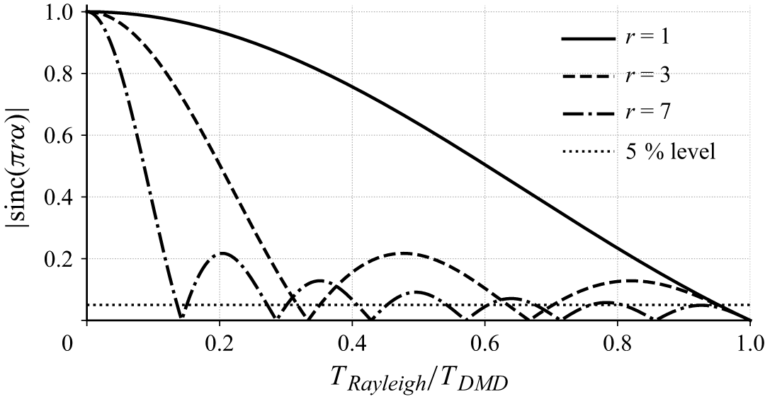
 |sinc(πrα)|
 α=TRayleigh/TDMD
 r
 r
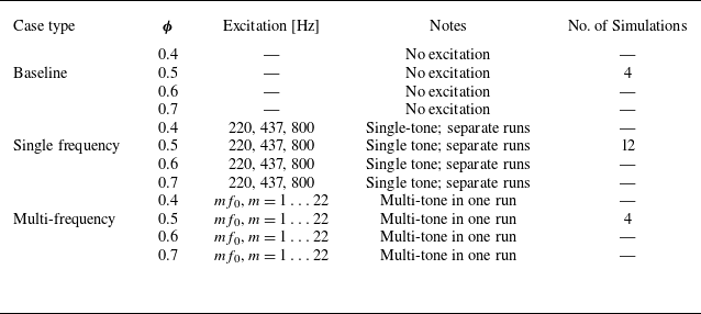
 ϕ
 f0=50Hz
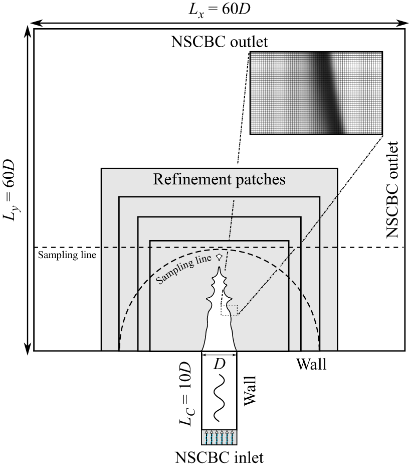

 q˙
 ϕ
 ϕ=0.4,0.5,0.6,0.7
 fexc=
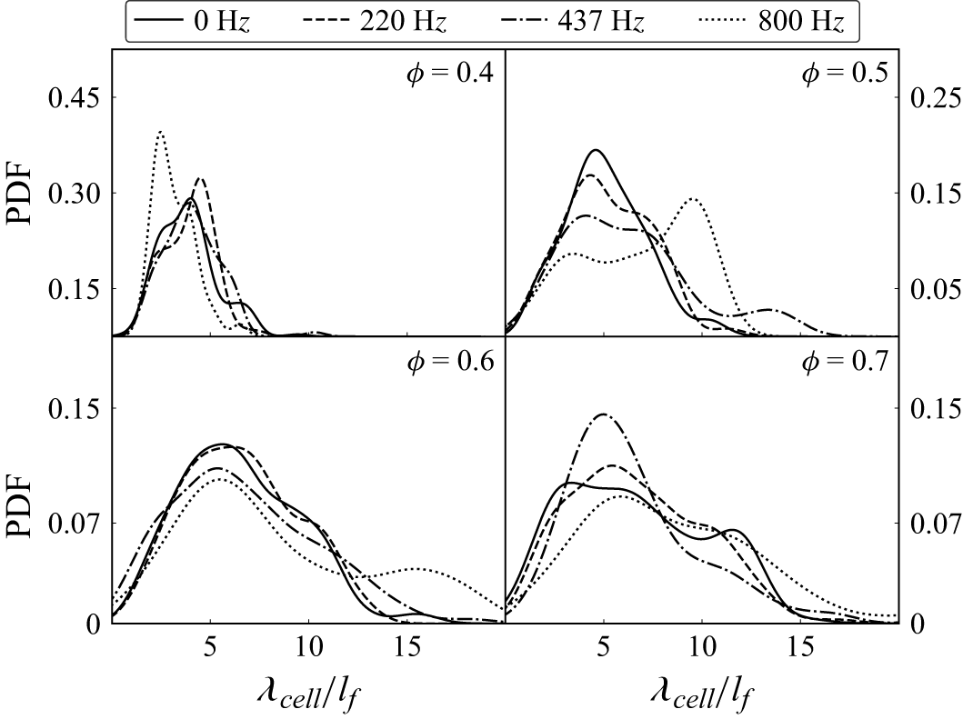
 λcell/lf
 ϕ=0.4,0.5,0.6,0.7
 fexc=0,220,437
 800Hz
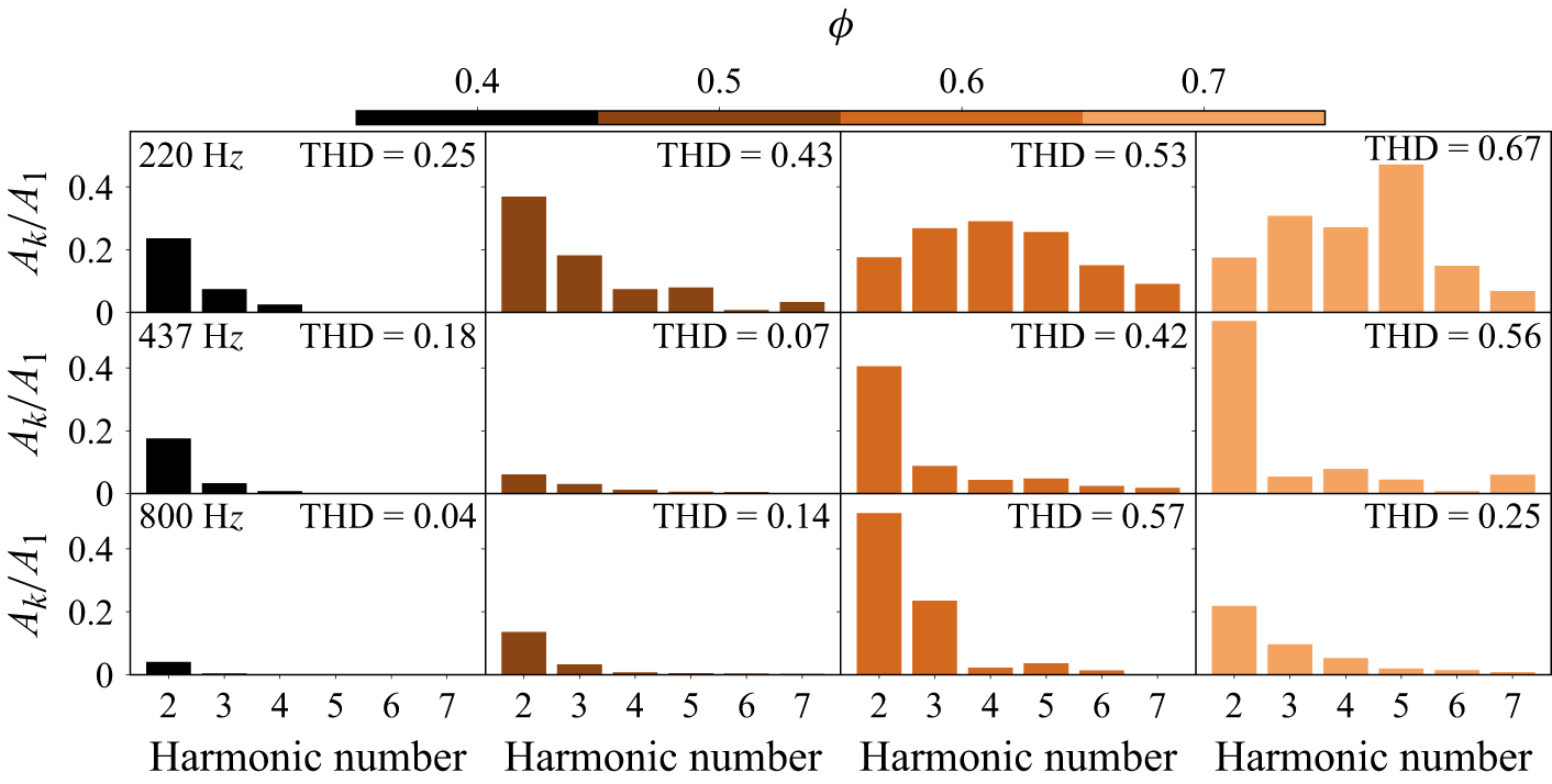
 fexc
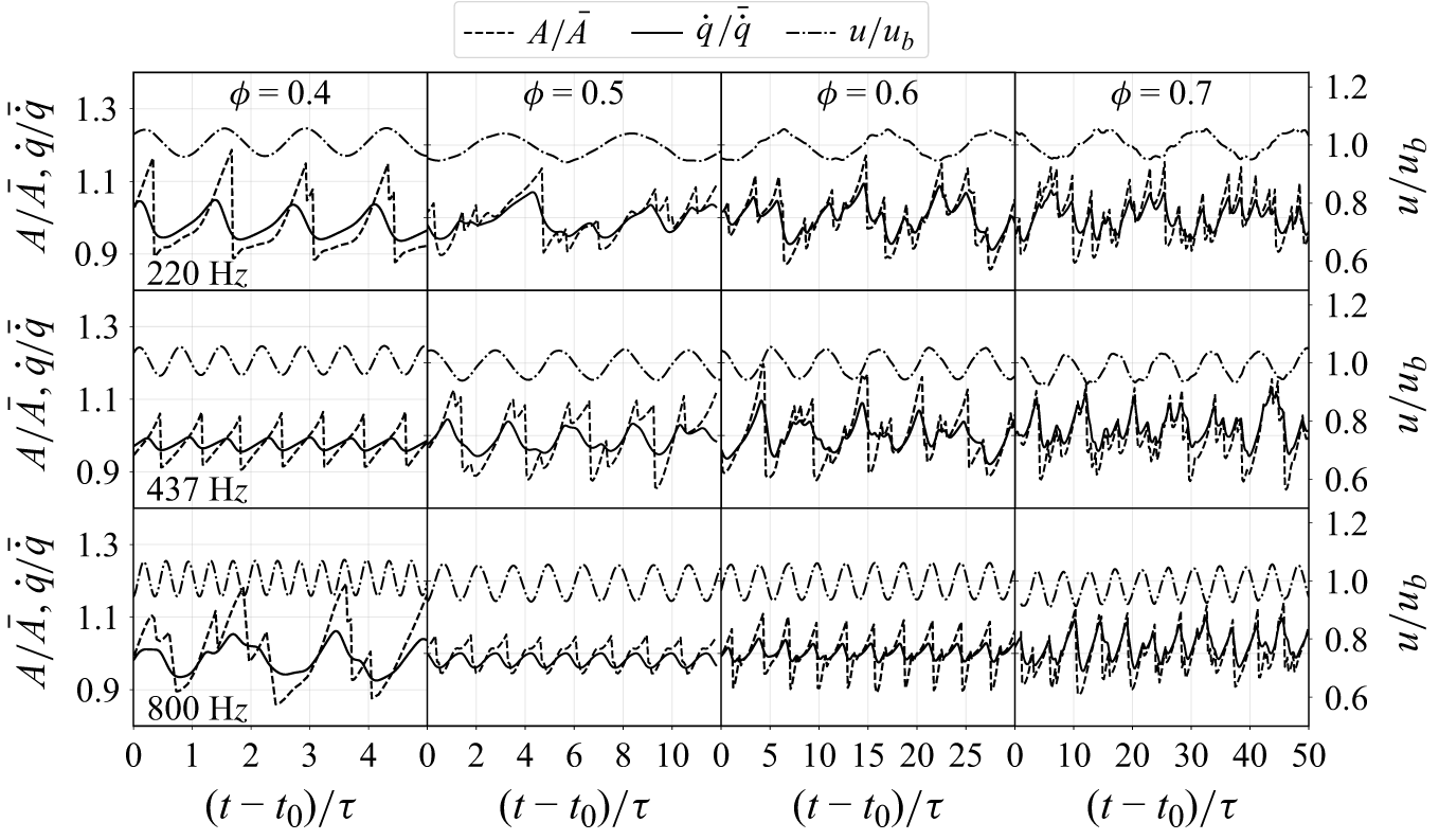
 q˙/q˙¯
 A/A¯
 u/ub
 ϕ=0.4,0.5,0.6,0.7
 t0
 τ

 q˙
 ∘
 ∘
 ∘
 ∘
 ∘
 ϕ=0.4
 ϕ=0.5
 ϕ=0.6
 ϕ=0.7
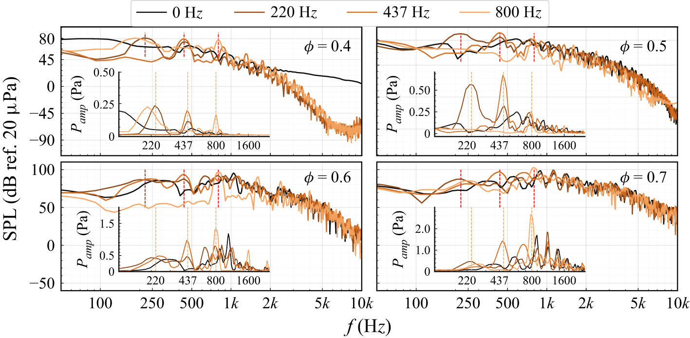
 ϕ=0.4,0.5,0.6,0.7
 μ
 Hz
 (Pamp)
 Hz
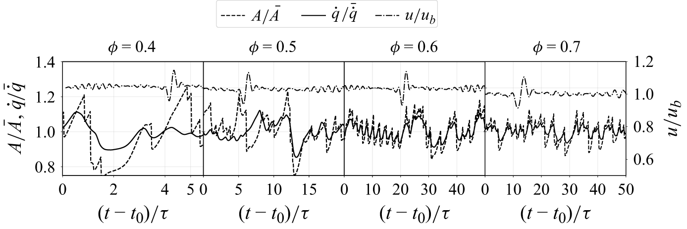
 q˙/q˙¯0
 A/A¯0
 u/ub
 ϕ=0.4,0.5,0.6,0.7
 t0
 τ
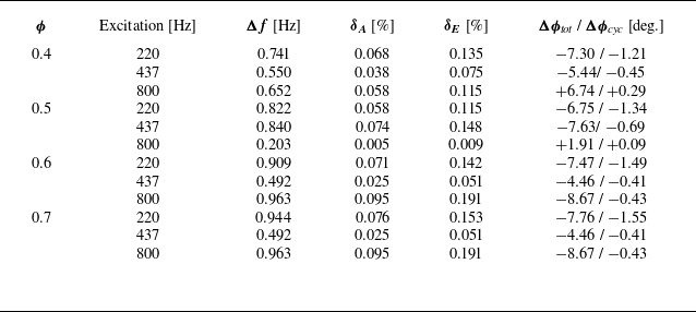
 ϕ
 Δf
 δA
 δE
 Δϕtot
 Δϕcyc
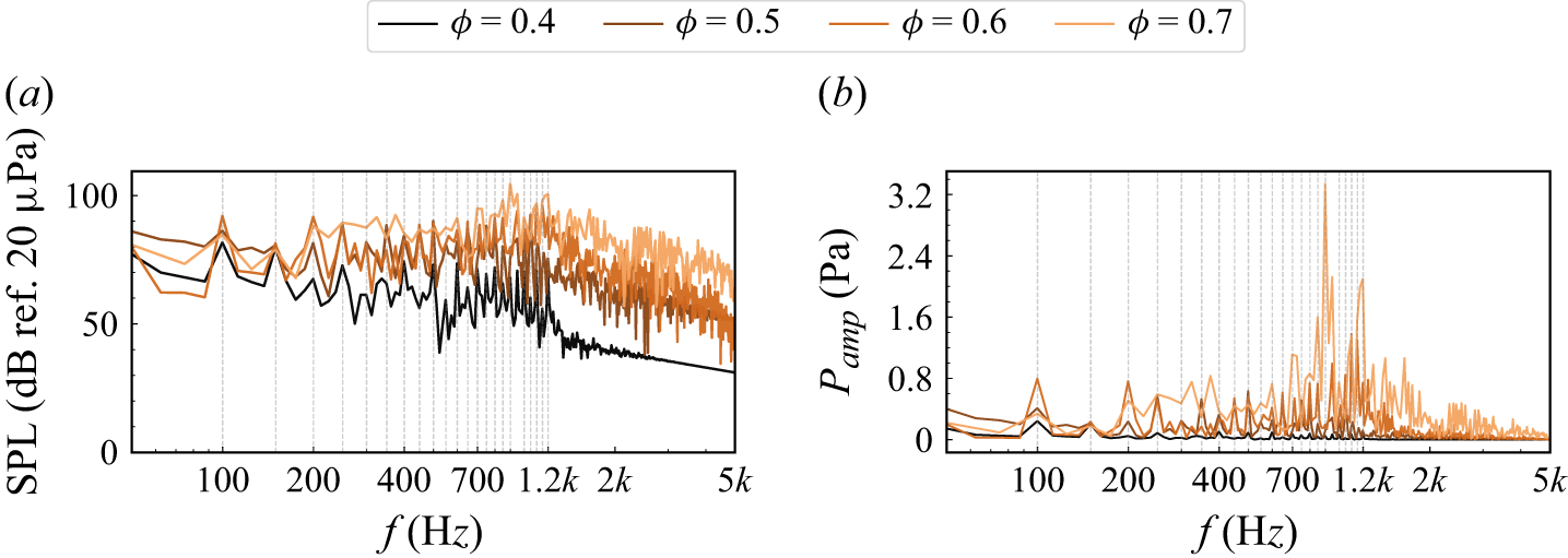
 ϕ=0.4.0.5,0.6,0.7
 μ
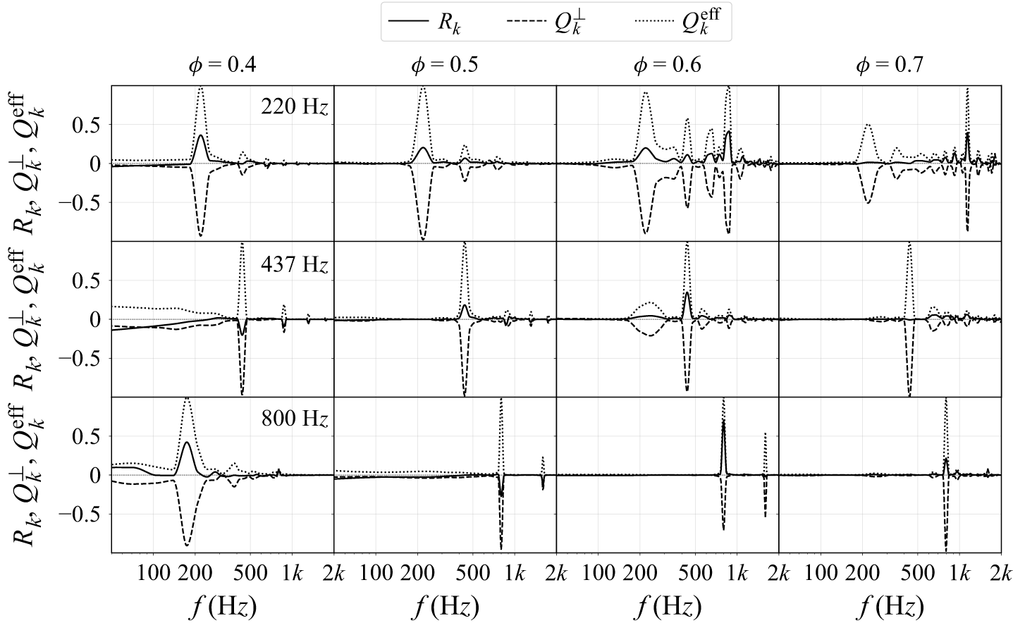
 R
 Q⊥
 ∘
 Qeff
 ϕ=0.4,0.5,0.6,0.7
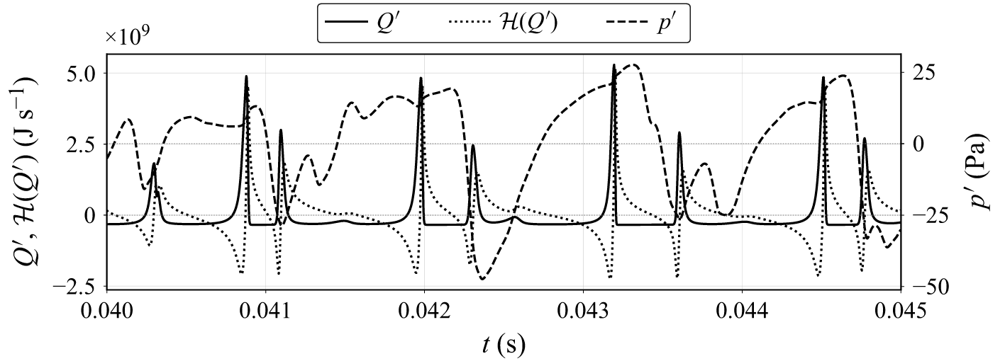
 Q′
 H(Q′)
 90∘
 p′
 ϕ=0.7,fexc=800Hz
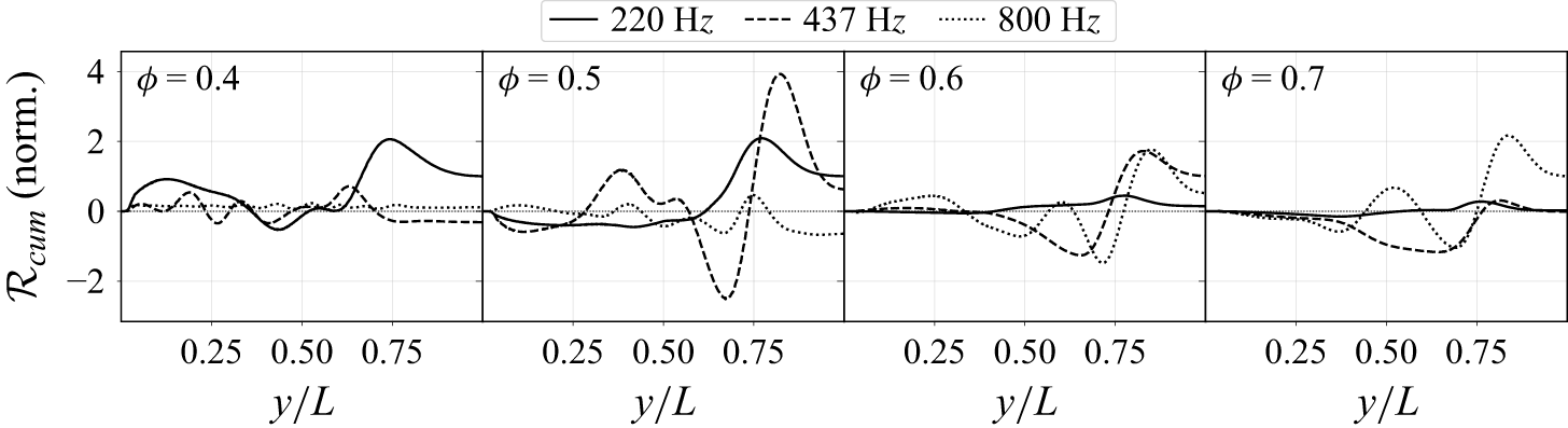
 y/L
 ϕ=0.4,0.5,0.6,0.7
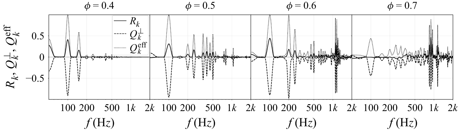
 R
 Q⊥
 ∘
 Qeff
 ϕ=0.4,0.5,0.6,0.7



